V2C-Long: Longitudinal Cortex Reconstruction with Spatiotemporal Correspondence

Abstract

Reconstructing the cortex from longitudinal MRI is indispensable for analyzing morphological changes in the human brain. Despite the recent disruption of cortical surface reconstruction with deep learning, challenges arising from longitudinal data are still persistent. Especially the lack of strong spatiotemporal point correspondence hinders downstream analyses due to the introduced noise. To address this issue, we present V2C-Long, the first dedicated deep learning-based cortex reconstruction method for longitudinal MRI. In contrast to existing methods, V2C-Long surfaces are directly comparable in a cross-sectional and longitudinal manner. We establish strong inherent spatiotemporal correspondences via a novel composition of two deep mesh deformation networks and fast aggregation of feature-enhanced within-subject templates. The results on internal and external test data demonstrate that V2C-Long yields cortical surfaces with improved accuracy and consistency compared to previous methods. Finally, this improvement manifests in higher sensitivity to regional cortical atrophy in Alzheimer’s disease.

1 Introduction

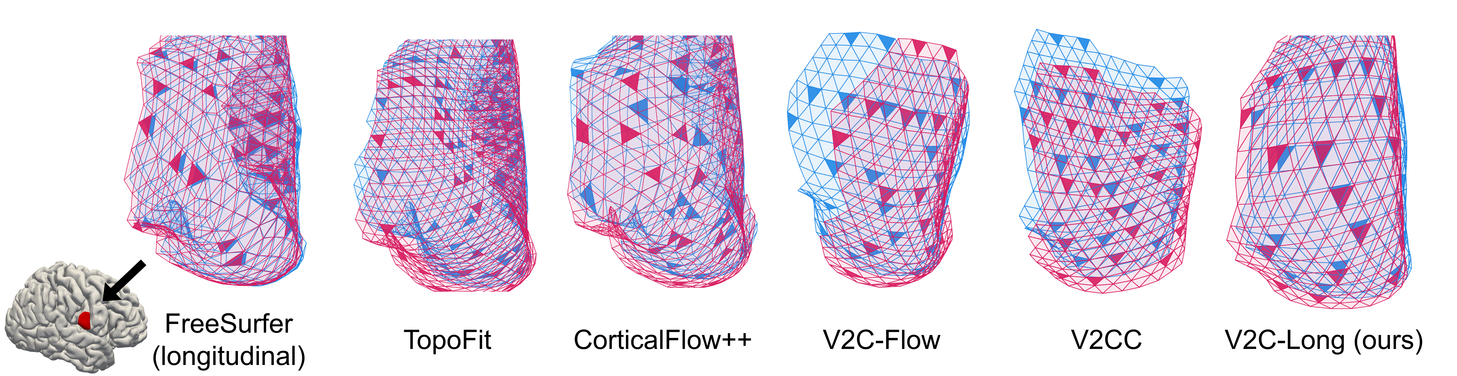
Figure 1: V2C-Long meshes are longitudinally consistent and regular — properties not jointly fulfilled by existing methods. We depict an exemplary right-hemisphere region of reconstructed pial surfaces from two timepoints (red and blue, respectively) of a subject in our ADNI test set. Ideally, colored triangles should match.

The structure of the cerebral cortex, i.e., the thin and tightly folded sheet of neural tissue confined by inner white matter (WM) and outer pial surfaces, has direct implications for brain functionality [22]. Structural measurements like cortical thickness or curvature are important biomarkers to understand brain development [20] and to track the progression of brain disorders [27, 2]. For accurate measurements, triangular meshes representing the WM and pial surfaces are typically extracted since they are less susceptible to partial volume effects compared to voxel-based image segmentation [7]. Recently, the automatic reconstruction of cortical surfaces from magnetic resonance imaging (MRI) has been sped up from hours to seconds with deep-learning approaches that can be executed on the latest generation of GPUs [6, 12, 18, 15, 13, 4].

These neural networks focus on cross-sectional data, but studying within-subject changes in aging, disease, and treatment relies on longitudinal data. Processing longitudinal neuroimaging data requires dedicated tools to reduce bias and increase the sensitivity to subtle differences in follow-up visits, typically far below the scanner resolution of 1mm [24]. To this end, unbiased within-subject templates and homologous points, i.e., corresponding anatomical locations, must be estimated accurately to make a local comparison of brain morphometry possible [23]. The intricate processing steps of these existing approaches complicate the incorporation of new scans and the processing of large studies, challenges that may be overcome with advanced neural networks.

Contribution In this work, we introduce a novel cortex reconstruction method dedicated to longitudinal MRI — with strong inherent spatiotemporal correspondence of surface points. To this end, we propose to leverage neural deformation fields to compute within-subject templates directly on the surface level and to incorporate these within-subject templates into the training of a second deep deformation network. The learning-based approach together with the parallel execution on the latest generation of GPUs allows us to compute application-ready longitudinal sequences of cortical surfaces within seconds.

Related Work Deep learning-based cortex reconstruction methods can be categorized into template-based, segmentation-based, and implicit methods. Implicit [6, 12] and segmentation-based approaches [18] usually rely on marching cubes [17], which precludes a direct comparison of the predicted meshes on a per-vertex basis. Template-based methods [31, 15, 13, 4, 26, 25, 5], on the other hand, take a generic, topologically correct template mesh as input and deform it to individual brain contours. Previous work has shown that this approach establishes correspondences between the generic template and the predicted surfaces, allowing for direct cross-sectional analyses and atlas propagation [5, 25]. However, these methods do not provide longitudinally consistent meshes, cf. Figure 1. FreeSurfer [9] implements a dedicated pipeline for longitudinal cortical segmentation and surface reconstruction (FS-Long for brevity) [24]. Unfortunately, surfaces from FS-Long and other longitudinal methods [16, 1] are only comparable within a single subject, but not across individuals; this requires error-prone and time-consuming surface inflation, registration, and re-sampling [11].

2 Method

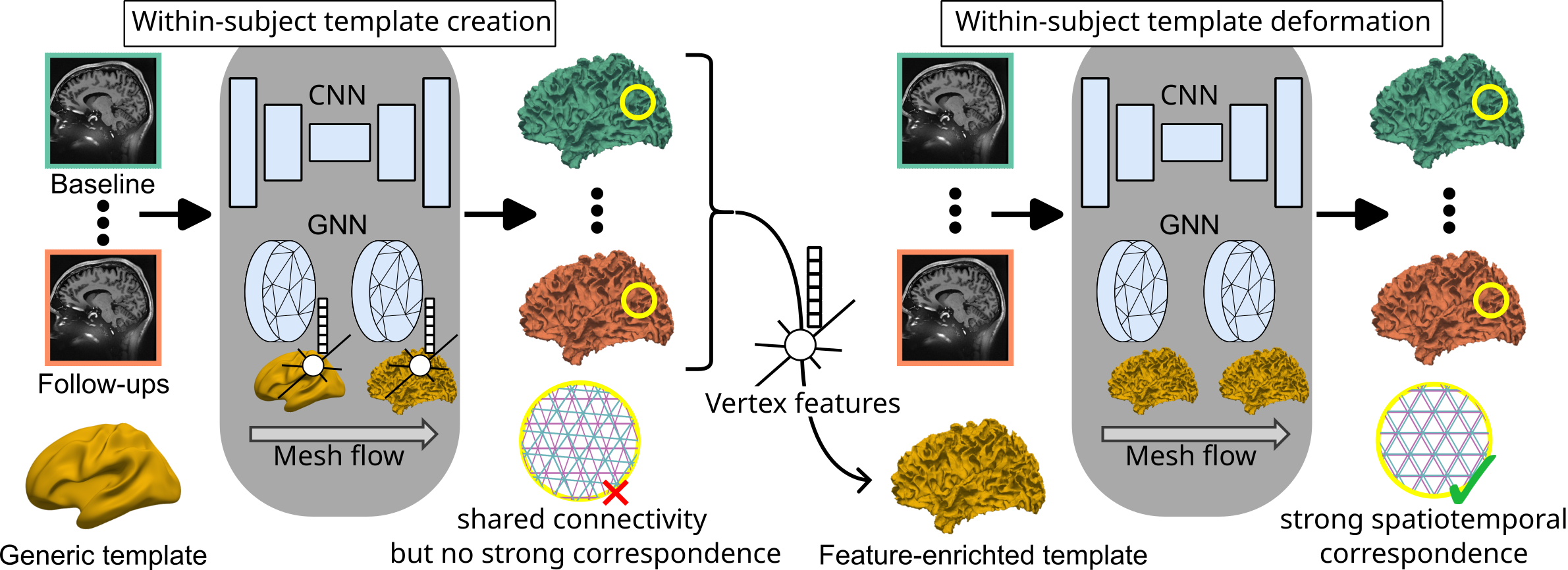
Figure 2: Architecture of V2C-Long. From a sequence of brain MRI scans, V2C-Long computes a within-subject template, enriches it with vertex features from a GNN, and deforms it to cortical surfaces with strong spatiotemporal point correspondence.

This section describes V2C-Long, a new method for fast reconstruction of longitudinally related cortical surfaces. As depicted in Figure 2, V2C-Long takes a sequence of 3D MR images $\{X_{ij}\,|\,j=0,\ldots,K_{i}\}$ from subject $i$ as input, where the number of follow-ups $K_{i}\geq 1$ can vary between subjects. WM and pial surfaces with spatial, i.e., between-subject, and temporal, i.e., within-subject, correspondence of anatomical points in all $K_{i}+1$ images are computed as output. We describe the two stages, within-subject template creation and subsequent within-subject template deformation, in Section 2.1 and Section 2.2, respectively. For a conceptual comparison with the longitudinal FreeSurfer processing, see Supplementary Figure 3. Throughout this work, we represent surfaces as closed triangular meshes $M=\{V,E\}$ with vertices $V$ and edges $E$.

2.1 Within-subject template creation

Within-subject templates condense multiple longitudinal snapshots of an individual’s brain into a single geometric model. These templates serve as a common ground for the local comparison and visualization of morphological measurements, e.g., cortical thickness. Their main purpose is to reduce within-subject noise and, thereby, increase the sensitivity since individual morphological changes are typically small compared to between-subject variations. To this end, FreeSurfer computes the median of intensity values after group-wise registration of a longitudinal sequence of scans [24]. However, this median image only serves as an intermediary step for cortex reconstruction.

We propose to compute the median directly on the cortical surfaces, i.e., on the mesh vertices that define these surfaces together with the edges. This is possible with meshes that share a common generic template, e.g., computed by V2C-Flow [5], whereas any application of marching cubes usually prevents such an operation. Compared to the group-wise image registration approach, aggregating the within-subject template from the vertices circumvents potential bias introduced by variations in voxel intensity or registration asymmetry [23]. Moreover, it is faster and facilitates the integration of newly acquired scans.

Given sets of vertices $\{V_{i,0},\ldots,V_{i,K_{i}}\}$ from subject $i$ at baseline and $K_{i}$ follow-up visits, in standard space with fixed order and connectivity such that $\nu=\lvert V_{i,j}\rvert=\lvert V_{i,k}\rvert\,\forall\,j,k\in\{0,\ldots,K_{i}\}$, we aggregate the within-subject mesh template $\mathcal{T}_{i}$ by computing the median of each vertex, i.e.,

$$\mathcal{T}_{i}=\text{med}({V_{i,0},\ldots,V_{i,K_{i}}}).$$ (1)

Since the median treats all timepoints equally, the resulting meshes are not biased toward any timepoint. Nonetheless, including all available timepoints in the aggregation is vital to avoid asymmetries. We experiment with V2C-Flow [5] and V2CC [25] for creating the within-subject template, cf. Section 3.3, as they offer the required fixed connectivity and inherent correspondence to a generic template (learned unsupervised in V2C-Flow and supervised in V2CC). This provides us with an even stronger relation than mentioned above, i.e., $\lvert V_{i,j}\rvert=\lvert V_{l,k}\rvert\,\forall\,i,j,k,l$, rendering the output surfaces and within-subject templates comparable between subjects. Thus, longitudinal group analyses of brain morphology can be conducted with the raw output of V2C-Long, cf. Section 3.4.

To enrich the templates with additional information about an individual’s cortex geometry, we concatenate the vertex features extracted by the two graph neural network (GNN) blocks in V2C-Flow to the vertex coordinates. These features contain geometric information beyond bare vertex coordinates as they guide the mesh flow, and we found them to improve the consistency of the reconstruction, cf. Section 3.3. Formally, we compute the median in Equation 1 from the resulting generalized vertices, which encompass both the spatial coordinates and the associated vertex features.

2.2 Within-subject template deformation

In the second stage of V2C-Long, the model learns to deform the within-subject template to the contours of a specific scan in order to establish a strong temporal correspondence among the surfaces of an individual. Notably, the template is only provided as a starting point, but the temporal deformation is not constrained further to avoid over-regularization [23]. The initial value problem

$$\frac{dV_{i,j}(t)}{dt}=f(t,I_{i,j},V_{i,j}(t));\quad V_{i,j}(0)=\mathcal{T}_{i}$$ (2)

formally defines the deformation from the individual template $\mathcal{T}_{i}$ to the cortical contours of the $j$-th scan of subject $i$, denoted as $I_{i,j}$, as an ordinary differential equation (ODE). Again, we employ V2C-Flow [5] to parameterize the deformation field $f:\mathbb{R}^{\nu\times 3}\rightarrow\mathbb{R}^{\nu\times 3}$ and use an Euler integration scheme with five integration steps to solve Equation 2. Compared to previous ODE-based cortex reconstruction [15, 5], however, we have a varying initial condition at $t=0$. We expect this augmentation to improve the generalization of the model.

2.3 Implementation details

We train the template-creation and template-deformation model sequentially for a maximum of 50 epochs each and choose the model weights with the lowest reconstruction error on the validation set. As training objective, we use 100,000 points randomly sampled from cross-sectional FreeSurfer meshes. Importantly, V2C-Long does not rely on the longitudinal FreeSurfer stream but instead learns longitudinal mesh correspondence unsupervised. The architecture, loss function, and optimizer for the template-creation and template-deformation model closely follow V2C-Flow [5]. We employ Nvidia A100 GPUs with 40GB memory, allowing for a batch size of one during training on one brain hemisphere.

3 Results

3.1 Experimental setting

For our experiments, we use T1 MRI scans from the longitudinal Alzheimer’s Disease Neuroimaging Initiative (ADNI, http://adni.loni.usc.edu), containing subjects with Alzheimer’s disease, mild cognitive impairment, and healthy controls. We split the data on the subject level and stratified our splits according to sex, age, and diagnosis at baseline. This results in 3,745, 594, and 1,094 scans for training, validation, and testing, respectively. Further, we use 288 scans (100 subjects) from the longitudinal OASIS-3 [14] study to evaluate the trained models externally. All data was pre-processed with FreeSurfer (v7.2) [9] and mapped to the MNI152 standard space (1mm, $182\times 218\times 182$ voxels) by affine registration [21] of the orig.mgz files. We compare our results to FS-Long (v7.2) [24], TopoFit [13], CF⁺⁺ [26], V2C-Flow [5], and V2CC [25], implemented consistently for the right brain hemisphere based on the original code repositories. Unless stated otherwise, we denote by V2C-Long the configuration with V2C-Flow templates and added vertex features.

3.2 Reconstruction consistency and accuracy

Table 1: Correspondence metrics by surface and method for the ADNI and OASIS test sets. Values are mean$\pm$std over all subjects and the best results are highlighted.

white surface pial surface both Model MCVar$\downarrow$ ParcF1$\uparrow$ MCVar$\downarrow$ ParcF1$\uparrow$ CThVar$\downarrow$ ADNI V2C-Long 0.020$\pm$0.020 0.971$\pm$0.015 0.012$\pm$0.015 0.966$\pm$0.017 0.016$\pm$0.010 V2C-Flow [5] 0.060$\pm$0.023 0.924$\pm$0.030 0.047$\pm$0.018 0.920$\pm$0.028 0.038$\pm$0.027 V2CC [25] 0.032$\pm$0.009 0.958$\pm$0.016 0.028$\pm$0.009 0.945$\pm$0.018 0.021$\pm$0.009 CF⁺⁺ [26] 0.046$\pm$0.017 – 0.046$\pm$0.017 – 0.034$\pm$0.027 TopoFit [13] 0.049$\pm$0.018 0.912$\pm$0.050 0.050$\pm$0.020 0.903$\pm$0.050 0.031$\pm$0.014 FS-Long [24] 0.032$\pm$0.013 0.968$\pm$0.050 0.031$\pm$0.015 0.953$\pm$0.050 0.032$\pm$0.019 OASIS V2C-Long 0.021$\pm$0.007 0.963$\pm$0.016 0.013$\pm$0.005 0.953$\pm$0.019 0.016$\pm$0.007 V2C-Flow 0.064$\pm$0.021 0.911$\pm$0.020 0.050$\pm$0.017 0.904$\pm$0.022 0.036$\pm$0.015 V2CC 0.035$\pm$0.010 0.947$\pm$0.017 0.034$\pm$0.011 0.929$\pm$0.021 0.023$\pm$0.010 CF⁺⁺ 0.050$\pm$0.018 – 0.051$\pm$0.019 – 0.037$\pm$0.018 TopoFit 0.060$\pm$0.019 0.885$\pm$0.023 0.067$\pm$0.024 0.873$\pm$0.025 0.036$\pm$0.014 FS-Long 0.033$\pm$0.013 0.964$\pm$0.017 0.040$\pm$0.020 0.941$\pm$0.021 0.030$\pm$0.013

Table 2: Reconstruction metrics by surface and method for the ADNI and OASIS test sets. Values are mean$\pm$std over all scans in mm (unless for SIF) and the best non-FreeSurfer results are highlighted.

white surface pial surface Model ASSD $\textsf{HD}_{90}$ %SIF ASSD $\textsf{HD}_{90}$ %SIF ADNI V2C-Long 0.177$\pm$0.161 0.410$\pm$0.756 0.64$\pm$0.38 0.174$\pm$0.161 0.409$\pm$0.731 2.15$\pm$0.92 V2C-Flow 0.186$\pm$0.116 0.427$\pm$0.644 1.01$\pm$0.39 0.180$\pm$0.109 0.419$\pm$0.566 2.44$\pm$0.90 V2CC 0.220$\pm$0.036 0.492$\pm$0.089 0.05$\pm$0.07 0.243$\pm$0.040 0.558$\pm$0.104 1.69$\pm$0.86 CF⁺⁺ 0.214$\pm$0.140 0.493$\pm$0.812 0.17$\pm$0.25 0.191$\pm$0.129 0.445$\pm$0.802 0.37$\pm$0.43 TopoFit 0.194$\pm$0.033 0.440$\pm$0.088 0.06$\pm$0.05 0.211$\pm$0.038 0.459$\pm$0.087 0.70$\pm$0.42 FS long. 0.151$\pm$0.089 0.317$\pm$0.187 0.00$\pm$0.00 0.145$\pm$0.078 0.300$\pm$0.221 0.00$\pm$0.01 OASIS V2C-Long 0.176$\pm$0.023 0.403$\pm$0.053 0.77$\pm$0.26 0.186$\pm$0.025 0.430$\pm$0.065 2.57$\pm$1.09 V2C-Flow 0.184$\pm$0.024 0.419$\pm$0.055 1.08$\pm$0.27 0.196$\pm$0.024 0.452$\pm$0.062 2.83$\pm$1.13 V2CC 0.222$\pm$0.036 0.506$\pm$0.082 0.04$\pm$0.06 0.282$\pm$0.044 0.654$\pm$0.116 1.95$\pm$0.94 CF⁺⁺ 0.226$\pm$0.032 0.522$\pm$0.078 0.21$\pm$0.13 0.210$\pm$0.041 0.473$\pm$0.078 0.47$\pm$0.22 TopoFit 0.197$\pm$0.026 0.447$\pm$0.065 0.07$\pm$0.05 0.228$\pm$0.036 0.502$\pm$0.086 0.88$\pm$0.47 FS-Long 0.126$\pm$0.024 0.264$\pm$0.053 0.00$\pm$0.00 0.132$\pm$0.025 0.274$\pm$0.055 0.00$\pm$0.00

Consistent cortex reconstruction is important since nonaligned meshes cause high noise levels in longitudinal measurements. To assess the consistency of reconstructed cortical surfaces from longitudinal MRI, we map the Destrieux [8] atlas, a fine-grained cortical atlas dividing the cortex into gyri and sulci, from FreeSurfer’s fsaverage to the predicted surfaces. This is possible for all methods except CF⁺⁺, which uses a custom template. We measure the overlap, i.e., the consistency, of segmented cortical regions in the longitudinal sequence with the average F1 score over all parcels (ParcF1). In addition, we compute the longitudinal variance of cortical thickness (CThVar) [10] and mean curvature [19] (MCVar) per vertex. Although the brain undergoes morphological change, regional variations of curvature (the cortical sheet is tightly folded) and thickness are usually greater than anatomical alterations over time [10]; hence, the variance in these measures should be smaller with better alignment. The results in Table 1 and Supplementary Figure 4 reveal a substantial improvement in consistency with V2C-Long over all baseline methods — including FS-Long. Qualitatively, we recognize in Figure 1 that V2C-Long is the only method that matches triangles from two different time points and accomplishes a regular mesh structure. FS-Long also provides matching triangles, but the meshes are distorted and less regular. The deep learning-based methods (TopoFit, CF⁺⁺, V2C-Flow, and V2CC), on the other hand, were developed for cross-sectional data and failed to provide longitudinally consistent meshes.

In Table 2, we evaluate the reconstruction accuracy of V2C-Long with respect to cross-sectional FreeSurfer surfaces, a standard in the field [6, 15, 4, 13]. We compute the average symmetric surface distance (ASSD) and robust 90-percentile Hausdorff distance (HD₉₀) to assess the surface accuracy, and we report the ratio of self-intersecting faces (SIF) to measure topological correctness. According to Table 2, V2C-Long yields the highest accuracy among all deep learning-based methods on the ADNI and OASIS test set. For the sake of completeness, we also include FS-Long in this comparison, although it intrinsically uses FreeSurfer methods and topology correction. V2C-Long does not achieve the lowest SIF scores but improves over its direct baseline V2C-Flow, which we attribute to a smoother deformation from the individual than the generic template.

3.3 Ablation studies

Table 3: Impact of the template creation and the vertex feature (VF)-enhancement on the surface quality and consistency. Values are mean$\pm$std on the ADNI test set.

white surface pial surface both Templates VF MCVar$\downarrow$ %SIF$\downarrow$ MCVar$\downarrow$ %SIF$\downarrow$ CThVar$\downarrow$ $\textsf{HD}_{90}$$\downarrow$ base img $\times$ .021$\pm$.008 1.062$\pm$.334 .013$\pm$.005 3.070$\pm$1.035 .017$\pm$.010 .398$\pm$.719 V2CC $\times$ .024$\pm$.009 0.344$\pm$.412 .016$\pm$.006 2.526$\pm$1.100 .019$\pm$.008 .392$\pm$.078 V2C-Flow $\times$ .022$\pm$.027 0.649$\pm$.439 .013$\pm$.020 2.323$\pm$0.926 .018$\pm$.012 .401$\pm$.623 V2C-Flow $\checkmark$ .020$\pm$.020 0.643$\pm$.375 .012$\pm$.015 2.151$\pm$0.921 .016$\pm$.010 .410$\pm$.743

In Table 3, we compare different configurations of V2C-Long on the ADNI data. The comparison comprises within-subject templates created with V2C-Flow, V2CC, or FreeSurfer’s base image, and with or without vertex features from V2C-Flow’s GNN. First, we observe that the margins are small compared to the improvement over existing methods reported in Section 3.2. Hence, we conclude that V2C-Long can be used with various templates and is not sensitive to changes thereof. Still, we found the vertex features to positively impact the consistency of WM and pial surfaces and derived thickness measures. We further note that the V2CC templates slightly improve the reconstruction accuracy. However, the limitations of GPU VRAM impede using vertex features from all four deformations in V2CC for now. Finally, meshes extracted from FreeSurfer’s base images can also be used in V2C-Long. Although we did not observe any benefit, it might be convenient to integrate V2C-Long into existing neuroimaging pipelines that rely on these images. Interestingly, we also found a strong correlation between the displacement from the template to the reconstruction and the parcellation and thickness consistency (MCVar: $r=-0.95$ (WM), $r=-0.90$ (pial), CThVar: $r=0.83$; see also Supplementary Figure 1). This result underpins our approach of using within-subject templates to initialize the reconstruction as they reduce the displacement compared to the generic templates used in previous methods.

3.4 Longitudinal cortical thinning in Alzheimer’s disease

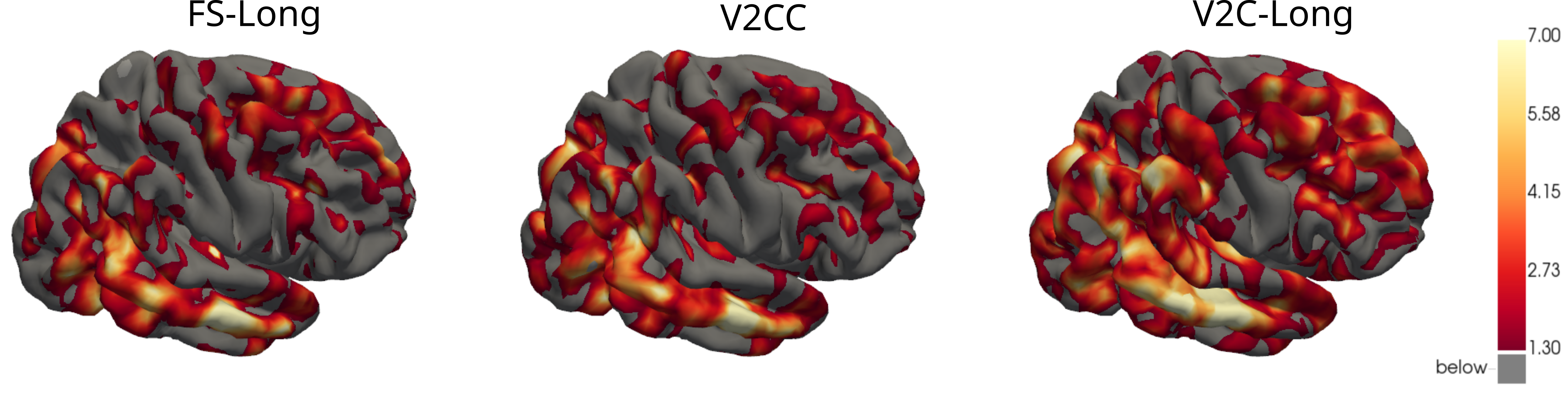
Figure 3: Differences in longitudinal cortical thickness between stable AD subjects ($n=71$) and healthy controls ($n=193$). We show uncorrected negative log10(p-value)-maps on fsaverage — based on meshes from FS-Long (v7.2), V2CC, and V2C-Long.

As a downstream analysis, we compare the pattern of longitudinal cortical thickness in patients affected by Alzheimer’s disease (AD) with a cognitively normal control group. To this end, we select $n=71$ AD subjects with a stable diagnosis and $n=193$ healthy controls from our ADNI test set. We perform a mass-univariate analysis of longitudinal cortical thickness (CTh) measurements with a vertex-wise linear mixed effects (LME) regression model [3, 30], i.e.,

$$\text{CTh}_{i,j}=\beta_{0}+\beta_{1}B_{i}+\beta_{2}W_{i,j}+\beta_{3}D_{i}+b_{0,i}+b_{1,i}W_{i,j}.$$ (3)

For subject $i$, this model considers the age at baseline visit $B_{i}$, the time $W_{i,j}$ from baseline to follow-up visit $j$, and the stable diagnosis $D_{i}$. It allows for individual intercepts and slopes via random effects regression coefficients $b_{0,i},b_{1,i}$. The fixed, non-individual regression coefficients $\beta_{0},\beta_{1},\beta_{2}$ model the global effects on cortical thickness. In Figure 3 and Supplementary Figure 2, we plot uncorrected two-tailed p-values of the t-statistics of the regression effect $\beta_{3}$, i.e., the diagnosis. All three methods, i.e., FS-Long, V2CC, and V2C-Long, highlight similar regions in the temporal and frontal lobes, which is consistent with the cortical atrophy, i.e., thinning, in Alzheimer’s reported in the literature [29]. However, the regions highlighted by V2C-Long have larger extent and are less fragmented, implying stronger statistical power and higher sensitivity compared to FS-Long and V2CC. Notably, we conducted this study with the raw V2C-Long output (FS-Long surfaces were inflated and re-sampled post hoc to fsaverage to be comparable between subjects), which reduces potential sources of error to a minimum. We used the LME implementation in statsmodels (v0.14.1) [28].

4 Conclusion

We introduced V2C-Long, the first dedicated deep-learning method for longitudinal cortex reconstruction and within-subject template creation. V2C-Long uses deep deformation fields to establish a strong inherent spatiotemporal correspondence between cortical surfaces, rendering them directly comparable without post-processing. Our experiments on two large longitudinal brain MRI studies validate the improved accuracy and consistency compared to previous methods. Eventually, we showed that these improvements lead to a higher sensitivity when quantifying cortical atrophy in patients affected by Alzheimer’s disease.

4.0.1 Acknowledgements

This research was partially supported by the German Research Foundation. We gratefully acknowledge the computational resources provided by the Leibniz Supercomputing Centre (www.lrz.de).

Supplementary Material

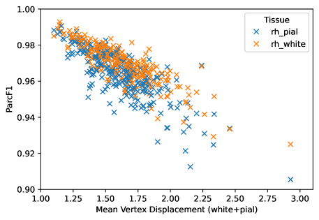
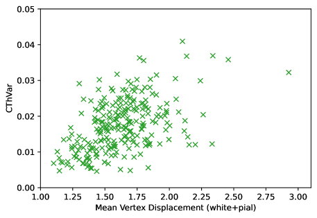
Supplementary Fig. 1: Mean vertex displacement vs. longitudinal consistency. Each cross represents a subject in the ADNI test set. One outlier was omitted for visual purposes.

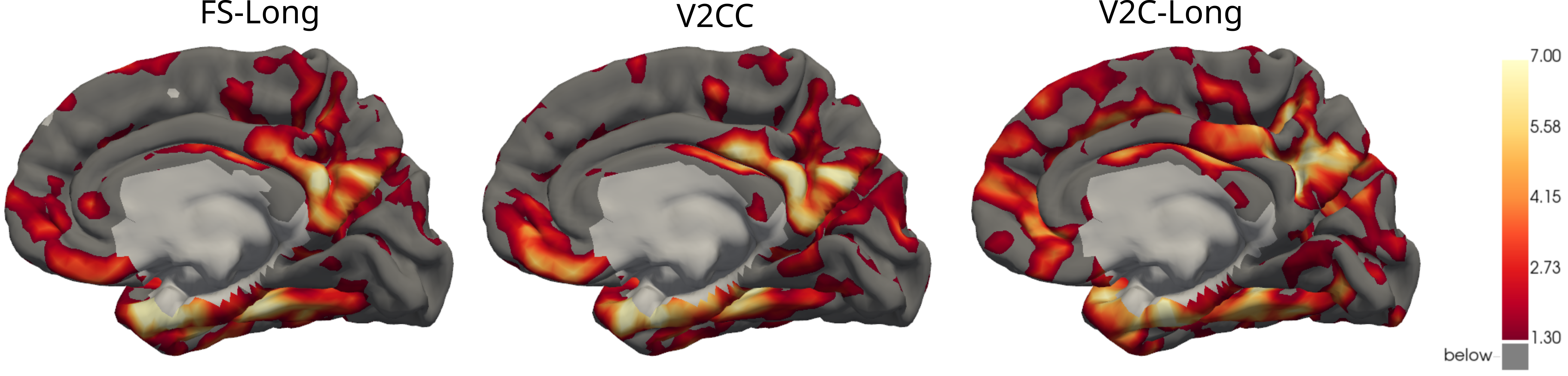
Supplementary Fig. 2: Sagittal view on the vertex-wise comparison of longitudinal cortical thickness between stable AD subjects and healthy controls in our ADNI test set.

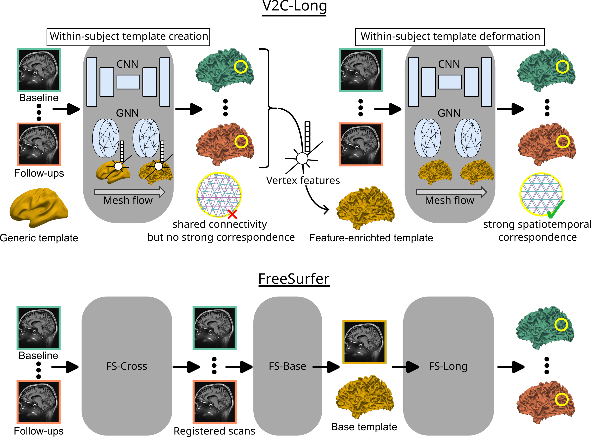
Supplementary Fig. 3: Conceptual comparison of V2C-Long with the longitudinal FreeSurfer pipeline.

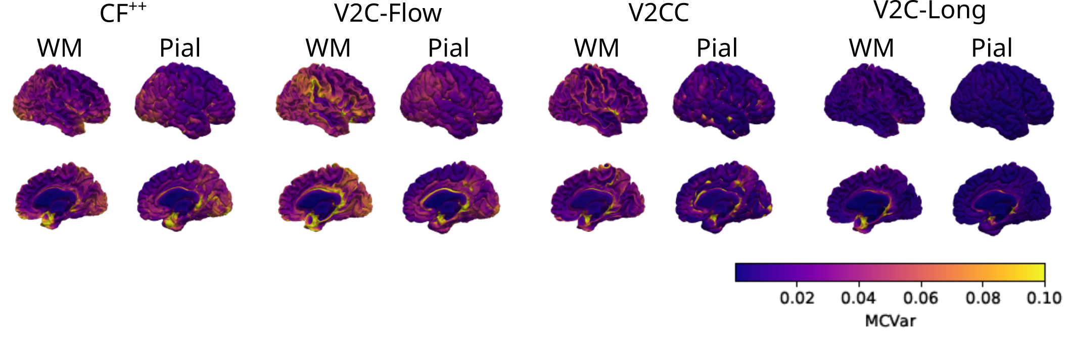
Supplementary Fig. 4: Vertex-wise mean curvature variance (MCVar) in our ADNI test set, obtained with V2C-Long and deep-learning baselines.

References

- [1] Ashburner, J., Ridgway, G.R.: Symmetric diffeomorphic modeling of longitudinal structural mri. Frontiers in Neuroscience 6 (2013)
- [2] Bachmann, T., Schroeter, M.L., Chen, K., Reiman, E.M., Weise, C.M.: Longitudinal changes in surface based brain morphometry measures in amnestic mild cognitive impairment and alzheimer’s disease. NeuroImage: Clinical 38, 103371 (2023)
- [3] Bernal-Rusiel, J.L., Greve, D.N., Reuter, M., Fischl, B., Sabuncu, M.R.: Statistical analysis of longitudinal neuroimage data with Linear Mixed Effects models. NeuroImage 66, 249–260 (2013)
- [4] Bongratz, F., Rickmann, A.M., Pölsterl, S., Wachinger, C.: Vox2cortex: Fast explicit reconstruction of cortical surfaces from 3d mri scans with geometric deep neural networks. In: Proceedings of the IEEE/CVF Conference on Computer Vision and Pattern Recognition (CVPR). pp. 20773–20783 (June 2022)
- [5] Bongratz, F., Rickmann, A.M., Wachinger, C.: Neural deformation fields for template-based reconstruction of cortical surfaces from mri. Medical Image Analysis 93, 103093 (Apr 2024)
- [6] Cruz, R.S., Lebrat, L., Bourgeat, P., Fookes, C., Fripp, J., Salvado, O.: Deepcsr: A 3d deep learning approach for cortical surface reconstruction. In: 2021 IEEE Winter Conference on Applications of Computer Vision (WACV). IEEE (Jan 2021)
- [7] Dale, A.M., Fischl, B., Sereno, M.I.: Cortical surface-based analysis. NeuroImage 9(2), 179–194 (Feb 1999)
- [8] Destrieux, C., Fischl, B., Dale, A., Halgren, E.: Automatic parcellation of human cortical gyri and sulci using standard anatomical nomenclature. NeuroImage 53(1), 1–15 (2010)
- [9] Fischl, B.: FreeSurfer. NeuroImage 62(2), 774–781 (2012)
- [10] Fischl, B., Dale, A.M.: Measuring the thickness of the human cerebral cortex from magnetic resonance images. Proceedings of the National Academy of Sciences 97(20), 11050–11055 (Sep 2000)
- [11] Fischl, B., Sereno, M.I., Dale, A.M.: Cortical surface-based analysis ii: Inflation, flattening, and a surface-based coordinate system. NeuroImage 9(2), 195–207 (Feb 1999)
- [12] Gopinath, K., Desrosiers, C., Lombaert, H.: SegRecon: Learning Joint Brain Surface Reconstruction and Segmentation from Images. In: MICCAI 2021, vol. 12907, pp. 650–659. Springer International Publishing (2021)
- [13] Hoopes, A., Iglesias, J.E., Fischl, B., Greve, D., Dalca, A.V.: Topofit: Rapid reconstruction of topologically-correct cortical surfaces. In: Medical Imaging with Deep Learning (2022)
- [14] LaMontagne, P.J., Benzinger, T.L., Morris, J.C., Keefe, S., Hornbeck, R., Xiong, C., Grant, E., Hassenstab, J., Moulder, K., Vlassenko, A.G., Raichle, M.E., Cruchaga, C., Marcus, D.: Oasis-3: Longitudinal neuroimaging, clinical, and cognitive dataset for normal aging and alzheimer disease. medRxiv (2019)
- [15] Lebrat, L., Santa Cruz, R., de Gournay, F., Fu, D., Bourgeat, P., Fripp, J., Fookes, C., Salvado, O.: Corticalflow: A diffeomorphic mesh transformer network for cortical surface reconstruction. In: Advances in Neural Information Processing Systems. vol. 34, pp. 29491–29505. Curran Associates, Inc. (2021)
- [16] Li, G., Nie, J., Wu, G., Wang, Y., Shen, D.: Consistent reconstruction of cortical surfaces from longitudinal brain mr images. NeuroImage 59(4), 3805–3820 (Feb 2012)
- [17] Lorensen, W.E., Cline, H.E.: Marching cubes: A high resolution 3d surface construction algorithm. ACM SIGGRAPH Computer Graphics 21(4), 163–169 (Aug 1987)
- [18] Ma, Q., Li, L., Robinson, E.C., Kainz, B., Rueckert, D., Alansary, A.: Cortexode: Learning cortical surface reconstruction by neural odes. IEEE Transactions on Medical Imaging 42(2), 430–443 (Feb 2023)
- [19] Meyer, M., Desbrun, M., Schröder, P., Barr, A.H.: Discrete differential-geometry operators for triangulated 2-manifolds. In: Visualization and Mathematics III. pp. 35–57. Springer Berlin Heidelberg, Berlin, Heidelberg (2003)
- [20] Mills, K.L., Tamnes, C.K.: Methods and considerations for longitudinal structural brain imaging analysis across development. Developmental Cognitive Neuroscience 9, 172–190 (Jul 2014)
- [21] Modat, M., Cash, D.M., Daga, P., Winston, G.P., Duncan, J.S., Ourselin, S.: Global image registration using a symmetric block-matching approach. Journal of Medical Imaging 1(2), 024003 (Sep 2014)
- [22] Pang, J.C., Aquino, K.M., Oldehinkel, M., Robinson, P.A., Fulcher, B.D., Breakspear, M., Fornito, A.: Geometric constraints on human brain function. Nature 618(7965), 566–574 (May 2023)
- [23] Reuter, M., Fischl, B.: Avoiding asymmetry-induced bias in longitudinal image processing. NeuroImage 57(1), 19–21 (2011)
- [24] Reuter, M., Schmansky, N.J., Rosas, H.D., Fischl, B.: Within-subject template estimation for unbiased longitudinal image analysis. NeuroImage 61(4), 1402–1418 (Jul 2012)
- [25] Rickmann, A.M., Bongratz, F., Wachinger, C.: Vertex Correspondence in Cortical Surface Reconstruction. In: MICCAI 2023, vol. 14227, pp. 318–327. Springer Nature Switzerland (2023)
- [26] Santa Cruz, R., Lebrat, L., Fu, D., Bourgeat, P., Fripp, J., Fookes, C., Salvado, O.: CorticalFlow++: Boosting Cortical Surface Reconstruction Accuracy, Regularity, and Interoperability, p. 496–505. Springer Nature Switzerland (2022)
- [27] Schwarz, C.G., Gunter, J.L., Wiste, H.J., Przybelski, S.A., Weigand, S.D., Ward, C.P., Senjem, M.L., Vemuri, P., Murray, M.E., Dickson, D.W., Parisi, J.E., Kantarci, K., Weiner, M.W., Petersen, R.C., Jack, C.R.: A large-scale comparison of cortical thickness and volume methods for measuring alzheimer’s disease severity. NeuroImage: Clinical 11, 802–812 (2016)
- [28] Seabold, S., Perktold, J.: statsmodels: Econometric and statistical modeling with python. In: 9th Python in Science Conference (2010)
- [29] Singh, V., Chertkow, H., Lerch, J.P., Evans, A.C., Dorr, A.E., Kabani, N.J.: Spatial patterns of cortical thinning in mild cognitive impairment and alzheimer’s disease. Brain 129(11), 2885–2893 (Sep 2006)
- [30] Wachinger, C., Salat, D.H., Weiner, M., Reuter, M.: Whole-brain analysis reveals increased neuroanatomical asymmetries in dementia for hippocampus and amygdala. Brain 139(12), 3253–3266 (Oct 2016)
- [31] Wickramasinghe, U., Remelli, E., Knott, G., Fua, P.: Voxel2Mesh: 3D Mesh Model Generation from Volumetric Data. In: MICCAI 2020, vol. 12264, pp. 299–308. Springer International Publishing (2020)