Leveraging Enhanced Queries of Point Sets for Vectorized Map Construction

Abstract

In autonomous driving, the high-definition (HD) map plays a crucial role in localization and planning. Recently, several methods have facilitated end-to-end online map construction in DETR-like frameworks. However, little attention has been paid to the potential capabilities of exploring the query mechanism. This paper introduces MapQR, an end-to-end method with an emphasis on enhancing query capabilities for constructing online vectorized maps. Although the map construction is essentially a point set prediction task, MapQR utilizes instance queries rather than point queries. These instance queries are scattered for the prediction of point sets and subsequently gathered for the final matching. This query design, called the scatter-and-gather query, shares content information in the same map element and avoids possible inconsistency of content information in point queries. We further exploit prior information to enhance an instance query by adding positional information embedded from their reference points. Together with a simple and effective improvement of a BEV encoder, the proposed MapQR achieves the best mean average precision (mAP) and maintains good efficiency on both nuScenes and Argoverse 2. In addition, integrating our query design into other models can boost their performance significantly. The code will be available at https://github.com/HXMap/MapQR.

1 Introduction

High-definition (HD) maps, essential for autonomous driving, encapsulate precise vectorized details of map elements such as pedestrian crossing, lane divider, road boundaries, etc. As a fundamental element of autonomous systems, these systems capture imperative road topology and traffic rules to support the navigation and planning of vehicles. Traditional SLAM-based HD map construction [35, 24] presents challenges such as complex pipelines, high costs, and notable localization errors. Manual annotation further intensifies the labor and time demands. These limitations are prompting a shift towards online, learning-based methods that utilize onboard sensors.

Many existing works [13, 36] define map construction as a semantic segmentation task in the bird’s eye view (BEV) space, producing rasterized maps. Although they have achieved much success, they face limitations due to extensive post-processing required to acquire vectorized information. To overcome the limitations of segmentation-based methods, new approaches have arisen that predict point sets to construct maps, utilizing a DETR-like structure for end-to-end map construction [18, 15, 16, 23, 6, 31].

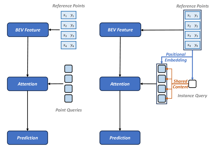
Figure 1: Comparison of overall architectures. Left: A DETR-like architecture exploited in many map construction methods. Right: The proposed architecture with scatter-and-gather query and positional embedding. To ensure consistency of content in a same map element, a scatter of instance queries is utilized to share content information. In addition, reference points are used for positional embedding of these queries, enabling the utilization of prior information.

The detection transformer (DETR) [2] is a transformer-based object detection architecture [26], in which learnable object queries are used to probe desirable information from image features. While the role of these learnable queries is still being studied, a common consensus is that a query consists of a semantic content part and a positional part. Thus corresponding objects can be recognized and localized in images [20, 17, 12, 34]. In Conditional DETR [20] and DAB-DETR [17], the positional part is explicitly encoded from reference points or box coordinates, which would then not be coupled with the content part and facilitate the learning process for both parts separately. These papers [20, 17] inspired us to design a proper query for point set prediction in the online map construction task.

DETR-like object detection methods predict a 4-dimensional bounding box information for each object by a set of learnable queries. As proved in DAB-DETR [17], each query in a decoder is composed of a decoder embedding (content information) and a learnable query (positional information). By contrast, HD map construction usually predicts a point set for each map element. In many state-of-the-art (SOTA) methods [15, 16, 6], point queries are used to probe information from BEV features, and each one predicts a point position. These predicted points are then grouped to form the detected map elements. Although information has been exchanged and enhanced in a self-attention module, it is still hard for a point query to contain all content information of the whole map element. In addition, point queries within the same map element may even have different semantic content information. We call this phenomenon as content conflicts. Therefore, previous point-query-based map construction methods have difficulty in learning desirable content information. In addition, current SOTA methods ignore the location information and simply use learnable queries that are randomly initialized.

To solve the aforementioned problem, we propose to use instance queries rather than point queries and add positional embedding, as shown in Fig. 1. Instead of predicting one position from each point query separately, we predict $n$ point positions simultaneously from each instance query to ensure consistency of content information in the same map element. To probe information from specific positions of BEV features, we generate positional embeddings from reference points like in Conditional DETR [20] (i.e., $n$ positional embeddings for each instance query). Then $n$ different positional embeddings will be added to each instance query, which becomes $n$ scattered queries. Therefore, each map element contains a group of scattered queries that share the same content part from a single instance query and different positional parts embedded from reference positions. The set of scattered queries is gathered back as an instance query to match a map element. We call this query a scatter-and-gather query. Since only instance queries are used as the input of a transformer decoder, it avoids content conflicts in the same map element. It also allows the proposed decoder to increase the number of queries to achieve higher accuracy without noticeably increasing the computational burden and memory usage. The query design is the fundamental cornerstone of our proposed method and, with a simple and effective improvement of a BEV encoder, constitutes our proposed MapQR.

We have performed extensive experiments to demonstrate the superiority of the proposed method MapQR. Our method has superior performance in both nuScenes and Argoverse 2 map construction tasks while maintaining good efficiency. Furthermore, we integrated the fundamental MapQR design into other SOTA models, substantially improving their final performance. In summary, the contributions of this paper are three-fold.

• We proposed an online end-to-end map construction method which is based on a novel scatter-and-gather query. This query design, coupled with a compatible positional embedding, is beneficial for point-set-based instance detection within DETR-like architectures.

• The proposed online map construction method performs better on existing online map construction benchmarks than prior arts.

• The incorporation of our core design into other SOTA online map construction methods also yields remarkable improvements in accuracy.

2 Related Work

2.1 Online Vectorized HD Map Construction

HD map is designed to encapsulate precise vectorized representation of map elements for autonomous driving. While conventional offline SLAM-based methods [35, 24] suffer from high maintaining cost, online HD map construction draws increasing attention. Online map construction can be solved by segmentation [22, 14, 36, 9] or lane detection [8, 3, 27] in BEV space, producing rasterized maps. HDMapNet [13] makes a further step of grouping segmentation results to vectorized representations.

VectorMapNet [18] proposes the first end-to-end vectorized map learning framework and utilizes auto-regression to predict points sequentially. Later end-to-end methods for vectorized HD map construction become popular [15, 16, 25, 23, 6, 30, 31, 32, 33]. MapTR [15] treats online map construction as a point set prediction problem and designs a DETR-like framework [2], achieving state-of-the-art performance. Its improved version MapTRv2 [16] designs a decoupled self-attention decoder and auxiliary losses to improve the performance further. Instead of representing a map element by a point set, BeMapNet [23] uses piecewise Bézier curve, and PivotNet [6] uses pivot-based points for more elaborate modeling. Most of these works use point-based queries and should meet the problem stated in Sec. 1. Recently, StreamMapNet [32] utilizes multi-point attention for a wide perception range and exploits long-sequence temporal fusion. Unlike previous work, we provide an in-depth exploitation of the instance-based query and design scatter-and-gather query to probe both content and positional information accurately.

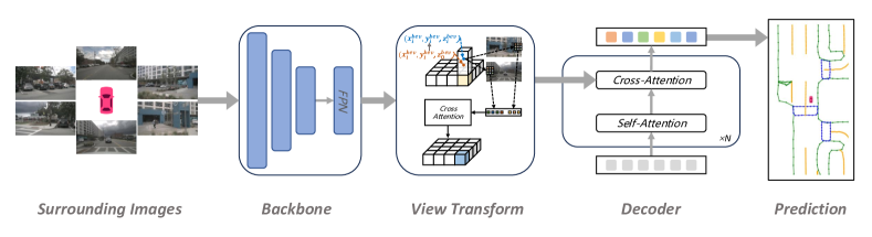
Figure 2: The overall architecture of our method. It contains three main components: a shared image backbone to extract image features, a view transformation module to obtain BEV features, and a transformer decoder for generating predictions. The backbone and view transformation modules can be any popular one without additional adaption. The decoder is our key design, and in principle it can be directly applied to other DETR-like models of map construction.

2.2 Multi-View Camera-to-BEV Transformation

HD map is commonly constructed under BEV view, and thus online HD map construction methods depend on converting visual features from camera perspective to BEV space. LSS [22] utilizes latent depth distribution to lift 2D image features to 3D space, and uses pooling later to aggregate to BEV features. BEVformer [14] depends on the transformer architecture [26] and designs spatial cross-attention based on visual projection. Unlike deformable attention [5] used in BEVformer, GKT [4] designs a geometry-guided kernel transformer. Besides, temporal information has also been explored to learn better BEV features [14, 21, 7]. All these methods can produce BEV features effectively, and our proposed decoder is compatible with all of them.

2.3 Detection Transformers

DETR [2] builds the first end-to-end object detector with transformer [26], eliminating the need for many hand-designed components. In the object detection task, it represents the object boxes as a set of queries, and directly uses the transformer encoder-decoder architecture to interact the queries with the image to predict the set of bounding boxes. Subsequent works [37, 37, 20, 28, 17, 12, 34] further optimize this paradigm and performance. In Deformable DETR [37], multi-scale features are incorporated to solve the problem of poor detection results of the vanilla DETR for small objects. In Conditional DETR [20] and DAB-DETR [17], the convergence of DETR is accelerated by adding positional embedding to learnable queries. In DN-DETR [12] and DINO [34], the actual boxes with noise are input into the decoder, so as to establish a more stable pairing relationship to accelerate convergence. The paradigm of DETR has been widely used in fields other than object detection tasks. For example, online vectorized HD map construction usually adopts DETR-like models [15]. Our model is also a DETR-like model. Leveraging point set representation of map elements, we design queries that can scatter and gather in a transformer decoder, and integrate positional information into the initialization of queries.

3 Method

3.1 Overall Architecture

The model of our method takes sequences of multi-view images as inputs to construct an HD map end-to-end, with the objective of generating sets of predicted points to represent instances of map elements. Each instance of a map element comprises a class label and a set of predicted points. Each predicted point includes explicit positional information to create polylines that represent the shape and location of the instance. The overall architecture of our model is shown in Fig. 2, which is similar in structure to other end-to-end models [18, 15].

Giving surrounding images from a multi-camera rig as inputs, we first extract image features through a shared 2D backbone. These image features of the cameras’ perspective view (PV) are converted to BEV representations by feeding into a view transformation module, commonly referred to as BEV encoder. The resulted BEV features are denoted as $F_{\mathrm{bev}}\in\mathbb{R}^{C\times H\times W}$, where $C$, $H$, $W$ represent the number of feature channels, height, and width, respectively. All mainstream 2D backbones [10, 19] and view transformation modules which can be used for PV-to-BEV transformation [4, 14] can be integrated into our model.

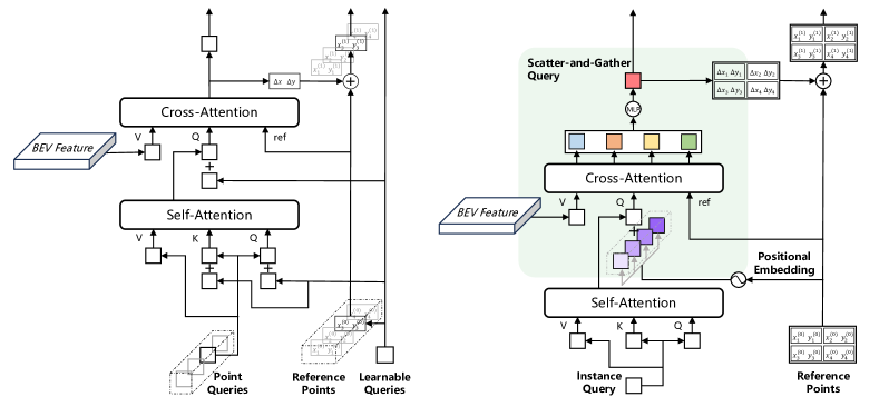
Figure 3: Comparison of decoders. Left: The decoder of MapTR [15]. Right: The proposed decoder of MapQR. In this example, $4$ reference points are contained in an instance.

3.2 Decoder with Scatter-and-Gather Query

The decoder of the architecture is our core design, consisting of stacked transformer layers, with its detail shown in Fig. 3. The improvements of our decoder mainly revolve around the query design, including the scatter-and-gather query and its compatible positional embedding.

Scatter-and-Gather Query. In our method, we propose using only one query type, instance query, as input to the decoder. We define a set of instance queries $\left\{q_{i}^{\mathrm{ins}}\right\}_{i=1}^{N}$, and each map element (with index $i$) corresponds to an instance query $q_{i}^{\mathrm{ins}}$. $N$ represents the number of instance queries, configured to exceed the typical number of map elements presenting in a scene. The $i$-th instance query $q_{i}^{\mathrm{ins}}$ is copied into $n$ scattered queries $\left\{q_{i,j}^{\mathrm{sca}}\right\}_{j=1}^{n}$ by an operator $\operatorname{scatter}$, i.e., $\left\{q_{i,j}^{\mathrm{sca}}\right\}_{j=1}^{n}=\operatorname{scatter}(q_{i}^{\mathrm{ins}})$. The operator $\operatorname{scatter}$ takes an input data vector and replicates it into multiple copies. Formally,

$$\operatorname{scatter}(f)=\underbrace{\{f,f,\ldots,f\}}_{n\ \text{replicas}},$$ (1)

where $n$ is the number of sequential points to model a map element. After passing through a transformer layer, scattered queries $\left\{q_{i,j}^{\mathrm{sca}}\right\}_{j=1}^{n}$ are aggregated into a single instance query using a $\operatorname{gather}$ operator, which is composed of an MLP as following:

$$\operatorname{gather}(\left\{f_{j}\right\}_{j=1}^{n})=\operatorname{MLP}(\operatorname{concat}(\left\{f_{j}\right\}_{j=1}^{n})).$$ (2)

The operator $\operatorname{concat}$ represents concatenation.

A complete decoder layer consists of a self-attention (SA) module and a cross-attention (CA) module. In each decoder layer, self-attention is used to exchange information between instance queries $\left\{q_{i}^{\mathrm{ins}}\right\}_{i=1}^{N}$. The output of self-attention is scattered into multiple copies, namely scattered queries $\left\{q_{i,j}^{\mathrm{sca}}\right\}_{i=1,j=1}^{N,n}$, and is used as input to cross-attention. The attention score is calculated with BEV features to probe the information from BEV space.

The detailed architectures of the proposed decoder with comparison to MapTR series [15, 16] are demonstrated in Fig. 3. MapTR [15] uses point queries as the input of decoder layers and calculates self-attention scores between them. This makes the computational complexity of self-attention much higher than our model because of much more involved queries.

By contrast, the proposed query design can ensure consistency of content in the same map element. Meanwhile, this design reduces the number of queries to reduce computational consumption in self-attention. Thus, it allows the involvement of more instance queries without significantly increasing memory consumption. Detailed experimental results are reported in Tab. 4.

Positional Embedding. As shown in Fig. 3, another key difference between the decoder of our model and other SOTA models is the usage of positional embedding. As demonstrated in DAB-DETR [17], a query is composed of a content part and a positional part. By designing a scatter-and-gather scheme of instance query, scattered queries corresponding to the same map element can share content information. Then another aspect that deserves exploration should be the positional information. In Conditional DETR [20] and DAB-DETR [17], the positional part is explicitly encoded from reference points or box coordinates so that it is not coupled to the content part and facilitates a learning process for both parts separately.

Considering the point set representation for the map construction task, we propose a more suitable way of positional embedding as shown in Fig. 3. In a decoder layer, each instance query $q_{i}^{\mathrm{ins}}$ is scattered into $n$ scattered queries $\left\{q_{i,j}^{\mathrm{sca}}\right\}_{j=1}^{n}$ after passing through the self-attention module. Each scattered query adds different positional embedding $P_{i,j}\in\mathbb{R}^{D}$ from its reference point $A_{i,j}=(x_{i,j},y_{i,j})$, where $x_{i,j},y_{i,j}\in\mathbb{R}$ are position coordinates, and $D$ is the dimension of query and positional embedding. The positional embedding $P_{i,j}$ of $j$-th scattered query is generated by:

$$P_{i,j}=\operatorname{LP}\left(\operatorname{PE}\left(A_{i,j}\right)\right),$$ (3)

where $\operatorname{LP}$ is a learnable linear projection, and $\operatorname{PE}$ means positional encoding to generate sinusoidal embeddings from float numbers. We overload the $\operatorname{PE}$ operator in the same way as DAB-DETR [17] to compute positional encoding of $A_{i,j}$:

$$\operatorname{PE}\left(A_{i,j}\right)=\operatorname{concat}\left(\operatorname{PE}\left(x_{i,j}\right),\operatorname{PE}\left(y_{i,j}\right)\right).$$ (4)

The positional encoding function $\operatorname{PE}$ maps a float number into a vector of $D/2$ dimensions as $\mathbb{R}\rightarrow\mathbb{R}^{D/2}$, and thus $\operatorname{PE}\left(A_{i,j}\right)\in\mathbb{R}^{D}$.

We have also tried adding positional embedding to instance query $q_{i}^{\mathrm{ins}}$ before self-attention modules, such as using learnable queries or encoding from the smallest bounding box covering the set of reference points. However, it did not achieve positive results, which are included in supplementary material. So, the positional embedding of the instance query is excluded in our model.

In summary, the calculation for $i$-th instance query in the scatter-and-collection query mechanism is

$$\operatorname{gather}\left(\operatorname{CA}\left(\operatorname{scatter}\left(\operatorname{SA}\left(q_{i}^{\mathrm{ins}}\right)\right)+\left\{P_{i,j}\right\}_{j=1}^{n},F_{\mathrm{bev}}\right)\right).$$ (5)

where $\left\{P_{i,j}\right\}_{j=1}^{n}$ are the set of positional embeddings. The resulted instance queries will be matched with the map elements to calculate the loss.

3.3 BEV Encoder: GKT with Flexible Height

BEV encoders learn to adapt to 3D space implicitly or explicitly. For example, BEVFormer [14] samples 3D reference points from fixed heights for each BEV query while learning adaptable offsets from projected 2D positions. Similar to BEVFormer, GKT [4] uses a fixed kernel to extract features around projected 2D image positions. Since GKT depends on a fixed 3D transformation, it lacks certain flexibility. Still, it has remarkable performance compared with BEVFormer [15].

To further increase the flexibility of GKT, we predict adaptive height offsets to original fixed heights when generating 3D reference points $\boldsymbol{p}_{i}=(x_{i}^{\mathrm{bev}},y_{i}^{\mathrm{bev}},z_{i}^{\mathrm{bev}})$ for each BEV query $q_{i}^{\mathrm{bev}}$:

$$z_{i}^{\mathrm{bev}}=z_{0}^{\mathrm{bev}}+\operatorname{LP}(q_{i}^{\mathrm{bev}}),$$ (6)

where offsets are predicted from query $q_{i}^{\mathrm{bev}}$ using a learable linear projection $\operatorname{LP}$, and 3D points $(x_{i}^{\mathrm{bev}},y_{i}^{\mathrm{bev}},z_{0}^{\mathrm{bev}})$ are sampled from BEV space as BEVFormer [14]. After projecting to 2D images, we still use a fixed kernel to extract features. We find this simple modification can further improve prediction results. It even outperforms BEVPoolv2 [11], which is used with auxiliary depth loss in MapTRv2. Its superiority with ablation study is demonstrated in experiments. We denote this improved GKT as GKT-h, in which the suffix ‘h’ stands for height.

3.4 Matching Cost and Training Loss

Our method uses hierarchical bipartite matching similar to the MapTR series [15, 16]. It is necessary to find the optimal instance assignment $\hat{\pi}$ between predicted map elements $\left\{\hat{y}_{i}\right\}_{i=1}^{N}$ and ground truth (GT) map elements $\left\{{y}_{i}\right\}_{i=1}^{N}$ as follows:

$$\hat{\pi}=\underset{\pi\in\Pi_{N}}{\arg\min}\sum_{i=1}^{N}\mathcal{L}_{\mathrm{ins\_match}}\left(\hat{y}_{\pi(i)},y_{i}\right),$$ (7)

where $\Pi_{N}$ is the set of permutations with $N$ elements. $\mathcal{L}_{\mathrm{ins\_match}}\left(\hat{y}_{\pi(i)},y_{i}\right)$ is a pair-wise matching cost between predictions $\left\{\hat{y}_{i}\right\}$ and GT map elements $\left\{{y}_{i}\right\}$. Then we use matching of scattered instances to find an optimal point-to-point assignment between the set of scattered instances and the set of GT points. The matching is established by calculating the Manhattan distance, which is the same as in MapTR.

The loss function is mainly consistent with MapTRv2 [16]. It is composed of three parts:

$$\mathcal{L}=\beta_{o}\mathcal{L}_{\text{one2one}}+\beta_{m}\mathcal{L}_{\text{one2many}}+\beta_{d}\mathcal{L}_{\text{dense}},$$ (8)

where $\beta_{o}$, $\beta_{m}$, and $\beta_{d}$ are the weights for balancing different loss terms. We set the same values as MapTRv2. The basic loss function $\mathcal{L}_{\text{one2one}}$ consists of three components: classification loss, point-to-point loss, and edge direction loss. Similarly, we repeat the ground-truth map elements $K$ times and fill them with the empty set $\varnothing$ to form a set of size $T$ to compute the auxiliary one-to-many set prediction loss $\mathcal{L}_{\text{one2many}}$. The auxiliary dense prediction loss $\mathcal{L}_{\text{dense}}$ differs from MapTRv2 due to its composition of two parts, as the BEV encoder of our method no longer predicts depth. Formally,

$$\mathcal{L}_{\text{dense }}=\alpha_{b}\mathcal{L}_{\text{BEVSeg}}+\alpha_{p}\mathcal{L}_{\text{PVSeg}},$$ (9)

where definitions of BEV segmentation loss and PV segmentation loss are the same as MapTRv2.

Since the proposed method mainly uses a novel design of query, we call the proposed method (scatter-and-gather query + positional embedding + GKT-h) as MapQR. Here QR is short for query. Sometimes we also want to emphasize the core contribution, i.e., the scatter-and-gather query with positional embedding. This part is denoted as SGQ for short.

Table 1: Comparison with SOTA methods on nuScenes. Our SGQ decoder is added to MapTR and MapTRv2 while keeps other settings, and the corresponding improvements are listed in brackets. FPS is tested on the same NVIDIA 4090 machine. The results in gray are taken from corresponding papers directly, and others are reproduced by ourselves. The best results for the same settings (i.e., backbone and epoch) are labeled in bold.

Method	Settings		APdiv	APped	APbou	mAP${}_{1}\uparrow$	APdiv	APped	APbou	mAP${}_{2}\uparrow$	FPS$\uparrow$ [t]
	Backbone	Epoch	{0.2m, 0.5m, 1.0m}				{0.5m, 1.0m, 1.5m}
BeMapNet [23]	R50	$30$	$46.9$	$39.0$	$37.8$	$41.3$	$62.3$	$57.7$	$59.4$	$59.8$	$8.3$ [t]
	R50	$110$	$52.7$	$44.5$	$44.2$	$47.1$	$66.7$	$62.6$	$65.1$	$64.8$	$8.3$
	SwinT	$30$	$49.1$	$42.2$	$39.9$	$43.7$	$64.4$	$61.2$	$61.7$	$62.4$	$7.9$ [b]
PivotNet [6]	R50	$24$	$41.4$	$34.3$	$39.8$	$38.5$	$56.5$	$56.2$	$60.1$	$57.6$	- [t]
	SwinT	$24$	$45.0$	$36.2$	$41.2$	$40.8$	$60.6$	$59.2$	$62.2$	$60.6$	- [b]
MapTR [15]	R50	$24$	$30.7$	$23.2$	$28.2$	$27.3$	$51.5$	$46.3$	$53.1$	$50.3$	${\bf 24.2}$ [t]
	R50	$110$	$40.5$	$31.4$	$35.5$	$35.8$	$59.8$	$56.2$	$60.1$	$58.7$	${\bf 24.2}$
	SwinT	$24$	$30.4$	$24.5$	$29.9$	$28.9$	$52.7$	$45.2$	$52.3$	$50.1$	${\bf 18.2}$
	SwinB	$24$	$36.5$	$29.0$	$35.2$	$33.5$	$58.7$	$50.6$	$58.4$	$55.9$	${\bf 9.3}$ [b]
MapTR +SGQ	R50	$24$	$38.4$	$31.6$	$33.2$	$34.4$(↑7.1)	$59.1$	$56.3$	$58.7$	$58.0$(↑7.7)	$22.4$ [t]
	R50	$110$	$46.7$	$39.4$	$39.9$	$42.0$(↑6.2)	$67.1$	$64.2$	$65.6$	$65.6$(↑6.9)	$22.4$
	SwinT	$24$	$37.9$	$31.2$	$33.9$	$34.3$(↑5.4)	$60.2$	$56.6$	$60.0$	$58.9$(↑8.8)	$17.3$
	SwinB	$24$	$41.0$	$31.9$	$36.7$	$36.5$(↑3.0)	$63.4$	$57.0$	$63.5$	$61.3$(↑5.4)	$9.0$[b]
MapTRv2 [16]	R50	$24$	$40.0$	$35.4$	$36.3$	$37.2$	$62.4$	$59.8$	$62.4$	$61.5$	$19.6$ [t]
	R50	$110$	$49.0$	$43.6$	$43.7$	$45.4$	$68.3$	$68.1$	$69.7$	$68.7$	[b]
MapTRv2 +SGQ	R50	$24$	$44.8$	$35.8$	$39.7$	$40.1$(↑2.9)	$63.7$	$60.3$	$66.1$	$63.4$(↑1.9)	$19.5$ [t]
	R50	$110$	$52.9$	$44.0$	$45.3$	$47.4$(↑2.0)	$69.8$	$67.7$	$70.4$	$69.3$(↑0.6)	[b]
MapQR (Ours)	R50	$24$	$49.9$	$38.6$	$41.5$	${\bf 43.3}$	$68.0$	$63.4$	$67.7$	${\bf 66.4}$	$17.9$ [t]
	R50	$110$	$57.3$	$46.2$	$48.1$	${\bf 50.5}$	$74.4$	$70.1$	$73.2$	${\bf 72.6}$	$17.9$
	SwinT	$24$	$49.3$	$38.5$	$41.1$	${\bf 43.0}$	$68.1$	$63.1$	$67.1$	${\bf 66.1}$	$14.8$
	SwinB	$24$	$52.3$	$41.4$	$43.2$	${\bf 45.6}$	$72.1$	$67.5$	$70.5$	${\bf 70.1}$	$8.3$

4 Experiments

We compare the proposed method MapQR with SOTA methods, including MapTR series [15, 16], BeMapNet [23] and PivotNet [6]. To validate the effectiveness of the proposed SGQ decoder separately, we also integrate it into the MapTR series by replacing their point-query-based decoders with the proposed decoder.

4.1 Settings

Datasets. We evaluate our method on popular self-driving datasets nuScenes [1] and Argoverse 2 [29]. These datasets provide surrounding images captured by self-driving cars in hundreds of city scenes. Each sample contains $6$ RGB images in nuScenes and $7$ RGB images in Argoverse 2. nuScenes provides 2D vectorized map elements, and Argoverse 2 provides 3D vectorized map elements as ground truth.

Evaluation Metric. Following previous works [13, 15], three static map categories are used for performance evaluation, i.e., lane divider, pedestrian crossing, and road boundary. Chamfer distance is used to determine whether the prediction matches the ground truth. Besides the thresholds $\{0.5m,1.0m,1.5m\}$ used in MapTR [15], the results are also evaluated with smaller thresholds $\{0.2m,0.5m,1.0m\}$ used in BeMapNet [23]. The corresponding mAP metrics are denoted as mAP₁ and mAP₂, respectively.

Training and Inference Details. We follow most settings as in the MapTR series [15, 16], and the modifications will be emphasized. The BEV feature is set to be $200\times 100$ to perceive [$-30m,30m$] for rear to front, and [$-15m,15m$] for left to right. We use $100$ instance queries to detect map element instances, and each instance is modeled by $20$ sequential points. (We set $N=100$ and $n=20$.)

Our model is trained on $8$ NVIDIA 4090 GPUs with a batch size of $8\times 4$. The learning rate is set to $6\times 10^{-4}$. We adopt ResNet50 [10] as the main backbone to compare with other methods. We also provide results with stronger backbones, including SwinB and SwinT [19].

4.2 Comparisons with State-of-the-art Methods

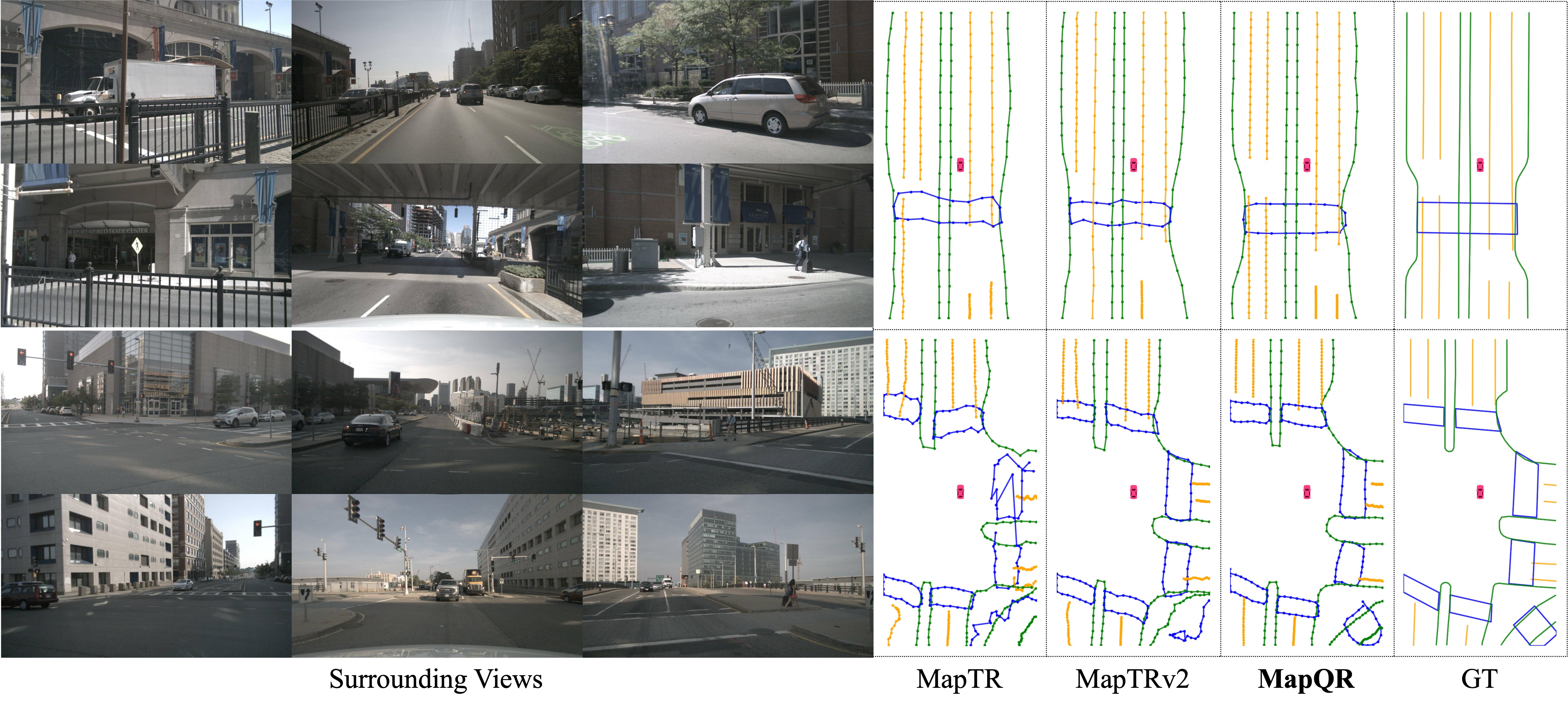
Figure 4: Comparison with SOTAs on qualitative visualization. The images are taken from the nuScenes dataset. The orange, blue and green colors represent lane divider, pedestrian crossing and road boundary, respectively. The proposed method obtains more accurate maps. The backbone R50 and $110$ epochs are used in all the methods.

Results on nuScenes. Following the previous experiment settings, 2D vectorized map elements are predicted by different methods. The experimental results are listed in Tab. 1. It can be seen that the proposed MapQR outperforms all other SOTA methods by a large margin for both mAP₁ and mAP₂, under the same settings (i.e., backbone and training epoch). Compared with MapTR and MapTRv2, BeMapNet [23] and PivotNet [6] get better results under smaller thresholds (i.e., mAP₁) thanks to their elaborate modeling. Still, the proposed method without elaborate modeling for map elements can outperform all of them. It implies that our instance query and improved encoder benefit for more accurate prediction. The inference speed of our method is about $18$ FPS, which meets the efficiency requirements of many scenarios.

To validate the effectiveness of the proposed SGQ decoder, it is integrated into both MapTR [15] and MapTRv2 [16], and all other settings except for the decoder are kept unchanged. The corresponding methods are denoted as MapTR+SGQ and MapTRv2+SGQ, respectively. Their performance and relative improvements are also listed in Tab. 1. For MapTR+SGQ, when trained with ResNet50 for $24$ epochs, our decoder helps to improve over $7.0\%$ mAP for both thresholds. Under other settings, the SGQ decoder can also enhance MapTR significantly. While MapTRv2 [16] uses decoupled self-attention in the decoder and some auxiliary supervision to improve results, simply replacing their decoder with ours can still step further, especially for the evaluation under stricter thresholds. For inference speed, introducing our decoder slows down only a little compared with original MapTR or MapTRv2.

Some qualitative results are shown in Fig. 4. In the first row, the comparison methods have acceptable results for forward sensing, while only the proposed method obtains satisfactory results for surround sensing. The second row demonstrates a complex intersection scenario. Our method obtains more satisfactory results than comparison methods. More results can be found in the supplementary materials.

Table 2: Comparison with SOTA methods on Argoverse 2. Map dim denotes the dimension used to model map elements. $dim=2$ indicates dropping the height of each predicted map elements, while $dim=3$ indicates predicting 3D map elements directly. The results in gray are taken from corresponding papers.

Methods	$dim$	mAP1	mAP2
PivotNet [6]	$2$	$40.7$	- [t]
MapTR [15]		$33.7$	$58.0$
MapTRv2 [16]		$42.0$	$67.4$
MapQR		${\bf 45.1}$	${\bf 68.2}$ [b]
MapTRv2 [16]	$3$	$38.4$	$64.7$ [t]
MapQR		${\bf 39.6}$	${\bf 65.9}$ [b]

Results on Argoverse 2. In Tab. 2, we provide the experimental results on Argoverse 2. These testings are all trained $6$ epochs with ResNet50 as the backbone. Since Argoverse 2 provides 3D vectorized map elements as ground truth, 3D map elements can be predicted directly ($dim=3$) as in MapTRv2. For both 2D and 3D prediction, the proposed MapQR achieves the best performance, especially for stricter thresholds (mAP₁). More detailed experimental results are included in the supplementary material.

4.3 Ablation Study

We present several ablation experiments for further analysis of our proposed method. All of these experiments are tested on nuScenes dataset with $24$ epochs.

Table 3: Ablations about scatter-and-gather query and positional embedding. Scatter & Gather denotes using scatter-and-gather queries. Pos. Embed. denotes positional embed. from reference points. The default settings for our method are highlighted.

Scatter & Gather	Pos. Embed.	mAP1	mAP2
-	-	$28.7$	$51.3$
-	✓	$29.9$	$52.6$
✓	-	$32.8$	$56.2$
✓	✓	${\bf 34.4}$	${\bf 58.0}$

Decoder Components. To further demonstrate the effectiveness of two components in our decoder, we provide an ablation study of scatter-and-gather query and positional embedding in Tab. 3. The first row corresponds to the original MapTR, which uses point queries and learnable positional embedding. In the second row, changing the learnable positional embedding to $\{P_{i,j}\}$ described by Eq. 3 can improve the performance. In the third row, using the proposed scatter-and-gather query instead of the point query improves the performance significantly. Finally, adding positional embedding $\{P_{i,j}\}$ of reference points can further improve the performance.

Table 4: Ablations about the number of instance queries ($N_{q}$). Mem. measures the memory usage for each GPU when training the networks. Blank denotes the values are not available due to the memory limit of NVIDIA 4090 (i.e., $24$ GB). The default settings for our method are highlighted.

Methods	$N_{q}$	mAP1	mAP2	Mem. (GB)
MapTR [15]	$50$	$27.3$	$50.3$	$13.46$ [t]
	$75$	$28.2$	$51.1$	$16.31$
	$100$	$28.7$	$51.3$	$20.44$
	$125$	-	-	- [b]
MapTR +SGQ	$50$	$32.1$	$55.9$	$11.27$ [t]
	$75$	$32.9$	$56.8$	$11.30$
	$100$	${\bf 34.4}$	${\bf 58.0}$	$11.51$
	$125$	$33.8$	$57.4$	$11.59$ [b]

Instance Query Number. We provide an ablation study about the instance query number $N$ in Tab. 4. The testings are based on our proposed decoder implemented in MapTR. For a fair comparison, we also provide the same ablation results for the original MapTR. The computation complexity of self-attention in its decoder is $O(N^{2})$. In our decoder, $N$ is the number of instance queries $N_{q}$. By contrast, in MapTR $N$ is the number of point queries, which is $N_{q}\times N_{p}$, and $N_{p}$ is the number of points to represent each instance. Therefore, as instance query number $N_{q}$ increases, the memory usage of MapTR increases dramatically. Although MapTRv2 has realized this problem and proposes a decoupled self-attention, it still consumes nearly all of the GPU memory ($24$ GB) even with $N_{q}=50$. In our decoder, lots of memory is saved since self-attention is only among instance queries. The memory usage has negligible increases as $N_{q}$ increases.

The performance of MapTR increases a little as $N_{q}$ increases, while our decoder obtains obviously better results for a proper larger $N_{q}$. When the same number of instance queries are used, our decoder outperforms MapTR. Since our method support a larger number of instance queries, we recommend using more instance queries than MapTR to obtain better results.

Table 5: Ablations about BEV encoder. BEVPool+ denotes using auxiliary depth supervision. GKT-h is our improved encoder.

BEV Encoder	mAP1	mAP2
BEVFormer [14]	$34.2$	$57.9$ [t]
BEVPool [11]	$31.2$	$55.0$
BEVPool+ [11]	$34.6$	$58.7$
GKT [4]	$34.4$	$58.0$
GKT-h	${\bf 35.5}$	${\bf 59.6}$ [b]

BEV Encoder. This ablation experiment is conducted on MapTR+SGQ by changing different BEV encoders. We test commonly used BEV encoders in Tab. 5. When one encoder layer is used in these BEV encoders, BEVFormer, BEVPool, PEVPool+, and GKT achieve comparable results. Our improved GKT with more flexible height sample locations, denoted as GKT-h, outperforms all other encoders obviously.

5 Conclusion

In this paper, we explore the query mechanism for better performance in online map construction task. Inspired by the frontier research in DETR-like architecture [20, 17], we design a novel scatter-and-gather query for the decoder. Therefore, in cross-attention, each point query for the same instance shares the same content information with different positional information, embedded from different reference points. We demonstrate the performance of SOTA methods can be further improved by combining them with our decoder. With our improvements in a BEV encoder, our new framework MapQR also achieves the best results in both nuScenes and Argoverse 2.

Supplementary Material

6 More Experimental Results

6.1 Detailed Experimental Results

In Tab. 6, Tab. 7, Tab. 8, and Tab. 9, more detailed experimental results are provided, including the average precision (AP) for lane divider, pedestrian crossing, and road boundary respectively. These results are consistent with Tab. 2 to Tab. 5 in the main manuscript.

6.2 Convergence Curve

We provide the training convergence curves in Fig. 5. Like the MapTR series, the proposed MapQR has converged when trained $110$ epochs, and achieves obviously better performance than MapTR [15] and MapTRv2 [16].

6.3 Ablation about Positional Embedding for Instance Queries

In Tab. 10, we provide an ablation study about the positional embedding for instance queries. This positional embedding is added to each instance query before self-attention, as illustrated in Fig. 6. We have tested some common choices for generating positional embedding (PE), including no PE, bounding box like in DAB-DETR [17], center point like in Conditional DETR [20], and learnable PE like in original MapTR [15]. The best results are obtained when no PE is used. Thus, we do not include any PE for instant queries in our model.

6.4 Ablation about Number of BEV Encoder Layer

As indicated in PivotNet [6], more encoder layers can also bring benefits. Thus we also provide an ablation study about the number of BEV encoder layer on MapQR in Tab. 11. As the number of layer increasing, the performance is also improved while with some cost of efficiency. To achieve an accuracy-and-efficiency trade-off, we set the layer number as $3$ for the default setting.

6.5 Qualitative Results

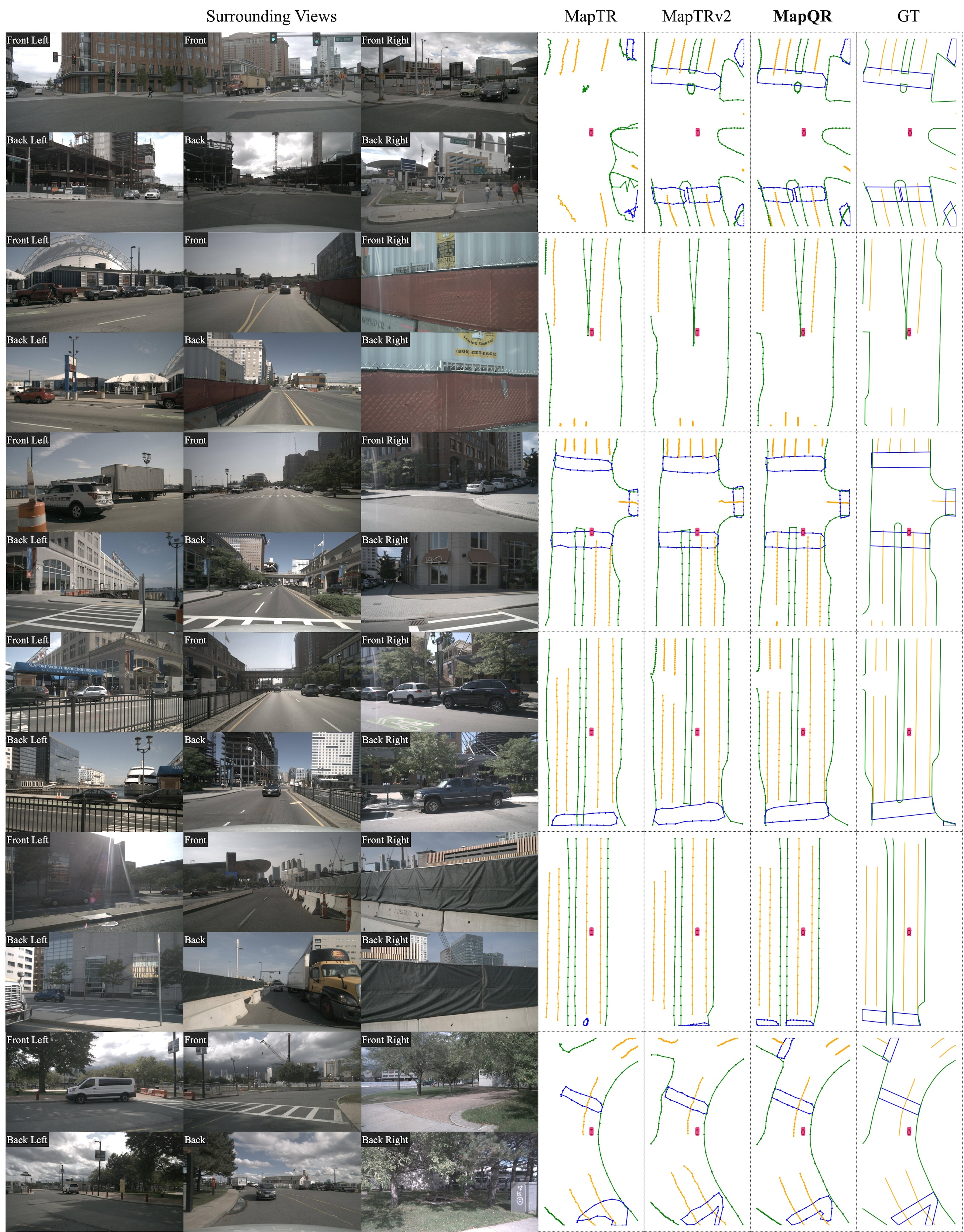
Figure 7: The orange, blue and green colors represent lane divider, pedestrian crossing and road boundary, respectively.

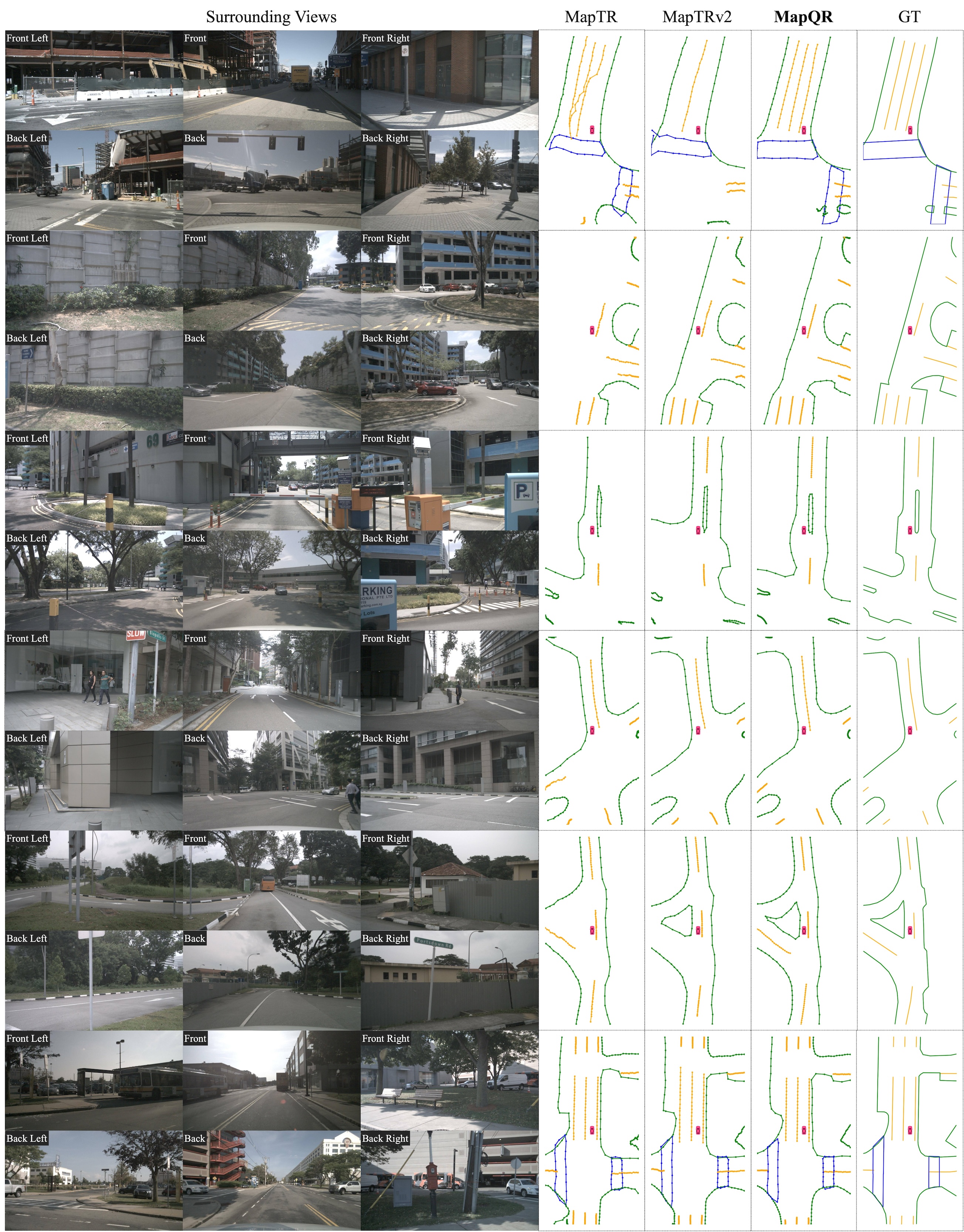
Figure 8: The orange, blue and green colors represent lane divider, pedestrian crossing and road boundary, respectively.

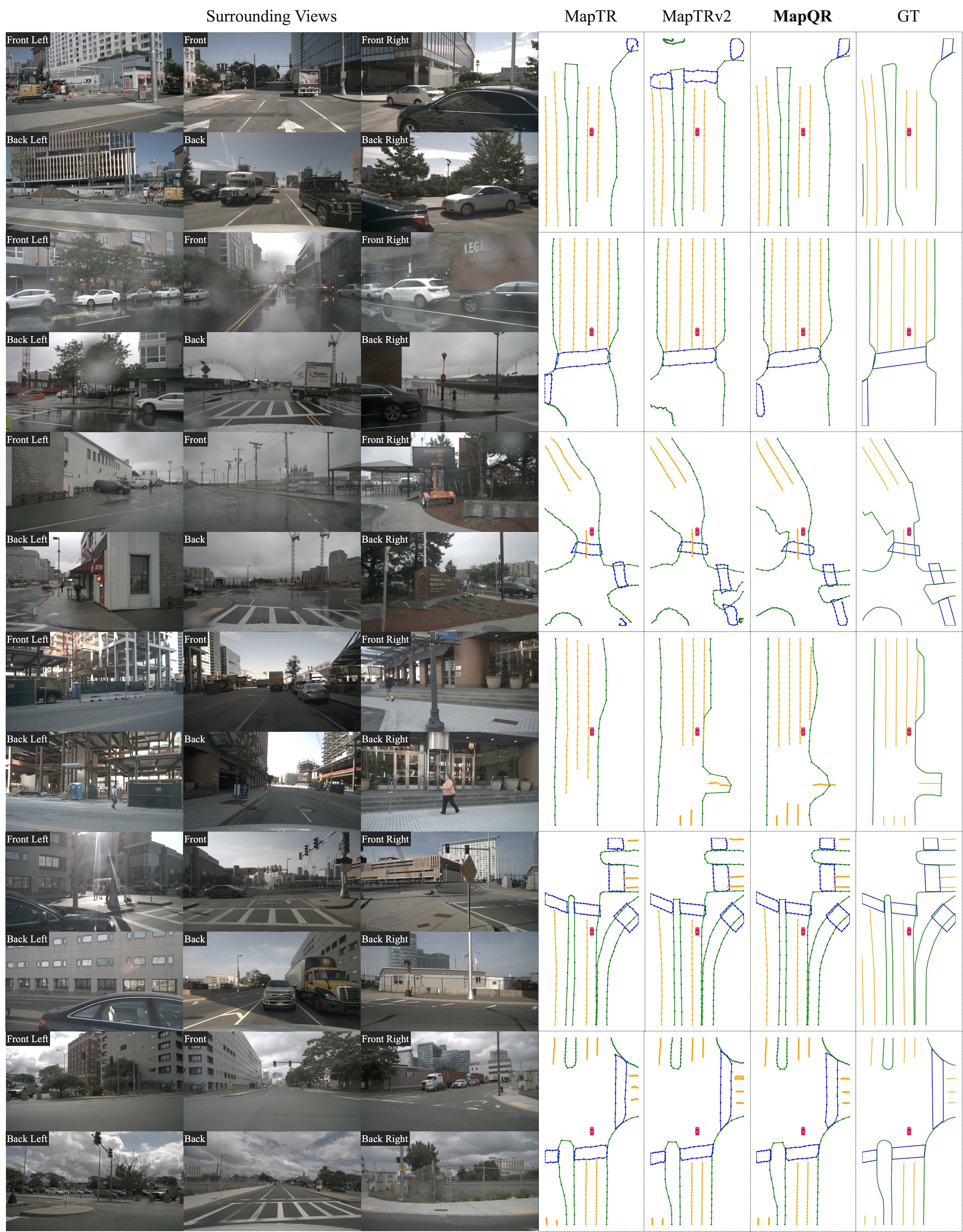
Figure 9: The orange, blue and green colors represent lane divider, pedestrian crossing and road boundary, respectively.

We provide more qualitative results on nuScenes [1] in Fig. 7, Fig. 8, and Fig. 9. For each example, the $3$ images in the first row are taken by the cameras of front-left, front, and front-right; the $3$ images in the second row are taken by the cameras of back-left, back, and back-right. For simple scenarios, all these methods can predict sufficiently accurate map elements. While for complex scenarios, MapQR predicts overall more accurate map elements with less false negatives and false positives.

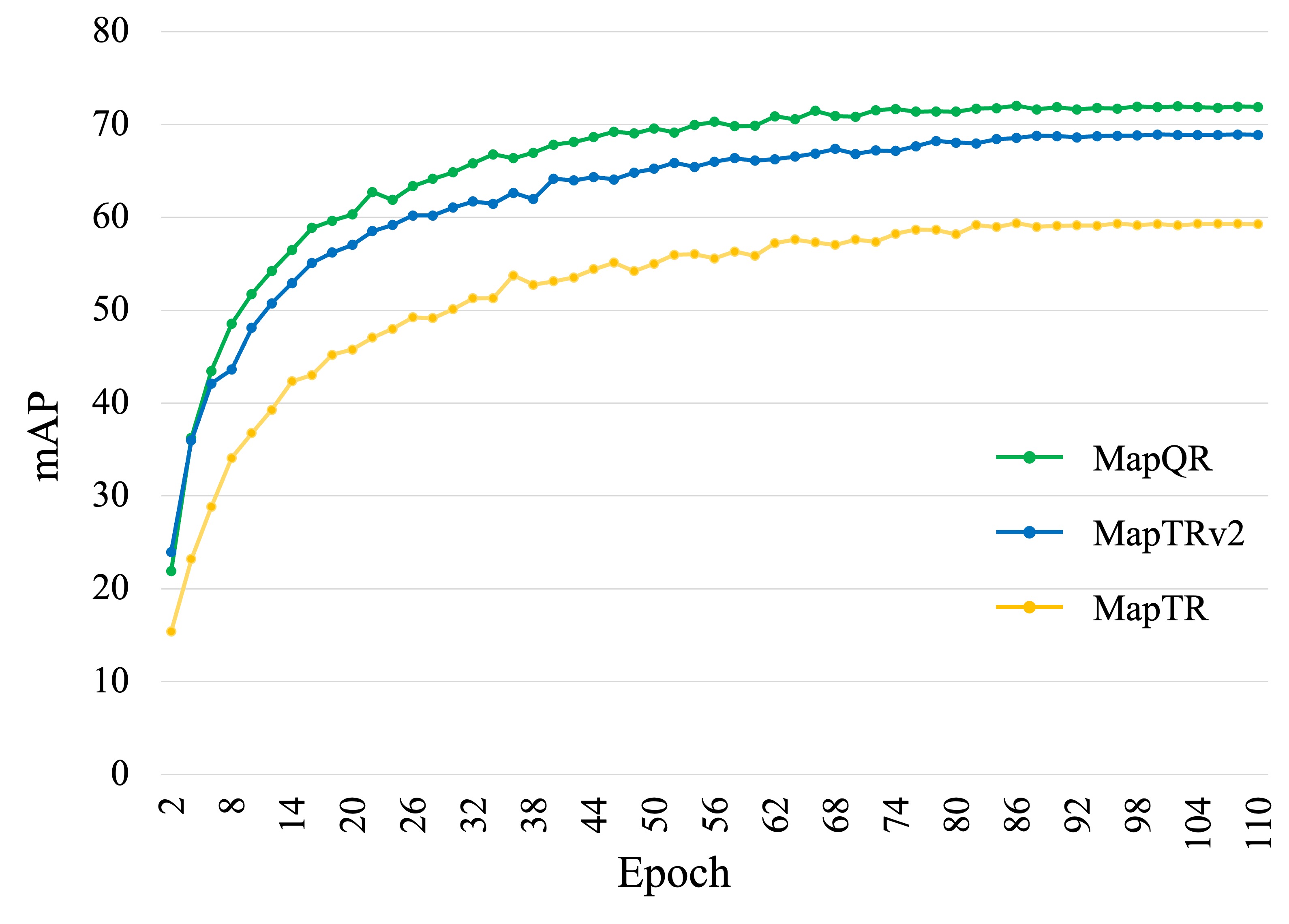
Figure 5: Convergence curves of MapQR, MapTR, and MapTRv2. These models are all trained 110 epochs, with ResNet50 as backbone.

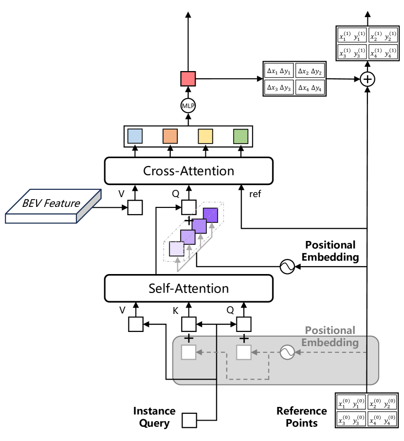
Figure 6: Structure of the proposed MapQR with positional embedding for instance queries, which is highlighted in the gray block. We do not use this positional embedding for the default setting.

Table 6: Comparison with SOTA methods on Argoverse 2. Map dim denotes the dimension used to model map elements. $dim=2$ indicates dropping the height of each predicted map elements, while $dim=3$ indicates predicting 3D map elements directly. The results in gray are taken from corresponding papers.

Methods	$dim$	APdiv	APped	APbou	mAP${}_{1}\uparrow$	APdiv	APped	APbou	mAP${}_{2}\uparrow$ [t]
		{0.2m, 0.5m, 1.0m}				{0.5m, 1.0m, 1.5m}
PivotNet [6]	$2$	$47.5$	$31.1$	$43.4$	$40.7$	-	-	-	-[t]
MapTR [15]		$40.5$	$27.9$	$32.9$	$33.7$	$56.9$	$57.9$	$59.2$	$58.0$
MapTRv2 [16]		$53.0$	$34.2$	$38.8$	$42.0$	$72.1$	$62.9$	$67.1$	$67.4$
MapQR		${56.3}$	${36.5}$	${42.5}$	${\bf 45.1}$	${72.3}$	${64.3}$	${68.1}$	${\bf 68.2}$ [b]
MapTRv2 [16]	$3$	$48.1$	$30.5$	$36.7$	$38.4$	$68.9$	$60.7$	$64.5$	$64.7$ [t]
MapQR		${49.4}$	${30.6}$	${38.9}$	${\bf 39.6}$	${71.2}$	${60.1}$	${66.2}$	${\bf 65.9}$ [b]

Table 7: Ablations about scatter-and-gather query and positional embedding. Scatter & Gather denotes using scatter-and-gather queries. Pos. Embed. denotes positional embed. from reference points. The default settings for our method are highlighted.

Scatter & Gather	Pos. Embed.	APdiv	APped	APbou	mAP${}_{1}\uparrow$	APdiv	APped	APbou	mAP${}_{2}\uparrow$ [t]
		{0.2m, 0.5m, 1.0m}				{0.5m, 1.0m, 1.5m}
-	-	$31.2$	$24.3$	$30.8$	$28.7$	$51.0$	$47.3$	$55.7$	$51.3$
-	✓	$32.3$	$26.1$	$31.3$	$29.9$	$52.7$	$48.9$	$56.0$	$52.6$
✓	-	$36.6$	$28.5$	$33.2$	$32.8$	$58.0$	$52.0$	$58.7$	$56.2$
✓	✓	$38.4$	$31.6$	$33.2$	${\bf 34.4}$	$59.1$	$56.3$	$58.7$	${\bf 58.0}$

Table 8: Ablations about the number of instance queries ($N_{q}$). Mem. measures the memory usage for each GPU when training the networks. Blank denotes the values are not available due to the memory limit of NVIDIA 4090 (i.e., $24$ GB). The default settings for our method are highlighted.

Methods	$N_{q}$	APdiv	APped	APbou	mAP${}_{1}\uparrow$	APdiv	APped	APbou	mAP${}_{2}\uparrow$	Mem. (GB) [t]
		{0.2m, 0.5m, 1.0m}				{0.5m, 1.0m, 1.5m}
MapTR [15]	$50$	$30.7$	$23.2$	$28.2$	$27.3$	$51.5$	$46.3$	$53.1$	$50.3$	$13.46$ [t]
	$75$	$31.2$	$23.2$	$30.1$	$28.2$	$51.8$	$46.3$	$55.3$	$51.1$	$16.31$
	$100$	$31.2$	$24.3$	$30.8$	$28.7$	$51.0$	$47.3$	$55.7$	$51.3$	$20.44$
	$125$	-	-	-	-	-	-	-	-	- [b]
MapTR +SGQ	$50$	$35.3$	$28.6$	$32.4$	$32.1$	$57.3$	$52.4$	$57.9$	$55.9$	$11.27$ [t]
	$75$	$36.8$	$28.9$	$32.9$	$32.9$	$58.4$	$53.7$	$58.4$	$56.8$	$11.30$
	$100$	${38.4}$	${31.6}$	${33.2}$	${\bf 34.4}$	${59.1}$	${56.3}$	${58.7}$	${\bf 58.0}$	$11.51$
	$125$	$38.9$	$29.2$	$33.2$	$33.8$	$59.8$	$53.4$	$59.0$	$57.4$	$11.59$ [b]

Table 9: Ablations about BEV encoder. BEVPool+ denotes using auxiliary depth supervision. GKT-h is our improved encoder.

BEV Encoder	APdiv	APped	APbou	mAP${}_{1}\uparrow$	APdiv	APped	APbou	mAP${}_{2}\uparrow$ [t]
	{0.2m, 0.5m, 1.0m}				{0.5m, 1.0m, 1.5m}
BEVFormer [14]	$39.3$	$29.6$	$33.8$	$34.2$	$60.1$	$54.0$	$59.7$	$57.9$ [t]
BEVPool [11]	$33.6$	$28.7$	$31.2$	$31.2$	$55.5$	$52.6$	$57.0$	$55.0$
BEVPool+ [11]	$36.8$	$31.7$	$35.2$	$34.6$	$58.5$	$56.0$	$61.5$	$58.7$
GKT [4]	${38.4}$	${31.6}$	${33.2}$	${34.4}$	${59.1}$	${56.3}$	${58.7}$	${58.0}$
GKT-h	${40.8}$	${31.4}$	${34.4}$	${\bf 35.5}$	${61.7}$	${56.6}$	${60.5}$	${\bf 59.6}$ [b]

Table 10: Ablations about positional embedding for instance queries. These experiments are tested on MapTR+SGQ. “Without” denotes not using any positional embedding, which is the default setting for our method. “Bounding Box” denotes embedding from the bounding boxes (i.e., $x,y,w,h$) of corresponding map instances. “Center Point” denotes embedding from only the center points (i.e., $x,y$) of corresponding bounding boxes. “Learnable” denotes using random learnable embedding.

Embedding Methods	APdiv	APped	APbou	mAP${}_{1}\uparrow$	APdiv	APped	APbou	mAP${}_{2}\uparrow$	FPS$\uparrow$ [t]
	{0.2m, 0.5m, 1.0m}				{0.5m, 1.0m, 1.5m}
Without	$38.4$	$31.6$	$33.2$	$\bf{34.4}$	$59.1$	$56.3$	$58.7$	$\bf{58.0}$	$22.4$ [t]
Bounding Box	$37.5$	$30.8$	$31.4$	$33.2$	$58.8$	$54.5$	$56.8$	$56.7$	$20.5$
Center Point	$37.4$	$28.6$	$31.2$	$32.4$	$58.8$	$53.2$	$56.6$	$56.2$	$21.2$
Learnable	${38.4}$	${30.4}$	${33.5}$	${34.1}$	${58.8}$	${55.5}$	${59.4}$	${57.9}$	$22.3$ [b]

Table 11: Ablations about the number of BEV encoder layers (#layer). The default settings for our method are highlighted.

#layer	APdiv	APped	APbou	mAP${}_{1}\uparrow$	APdiv	APped	APbou	mAP${}_{2}\uparrow$	FPS$\uparrow$ [t]
	{0.2m, 0.5m, 1.0m}				{0.5m, 1.0m, 1.5m}
1	$46.4$	$36.1$	$39.7$	$40.8$	$64.8$	$60.9$	$65.2$	$63.6$	$21.3$ [t]
2	$49.3$	$38.0$	$40.4$	$42.6$	$66.9$	$62.5$	$66.4$	$65.3$	$19.8$
3	$49.9$	$38.6$	$41.5$	$43.3$	$68.0$	$63.4$	$67.7$	$66.4$	$17.9$
4	${50.3}$	${39.9}$	${41.0}$	${43.8}$	${69.2}$	${65.6}$	${67.3}$	${67.4}$	$16.9$

References

- Caesar et al. [2020] Holger Caesar, Varun Bankiti, Alex H Lang, Sourabh Vora, Venice Erin Liong, Qiang Xu, Anush Krishnan, Yu Pan, Giancarlo Baldan, and Oscar Beijbom. nuScenes: A multimodal dataset for autonomous driving. In CVPR, pages 11621–11631, 2020.
- Carion et al. [2020] Nicolas Carion, Francisco Massa, Gabriel Synnaeve, Nicolas Usunier, Alexander Kirillov, and Sergey Zagoruyko. End-to-end object detection with transformers. In ECCV, pages 213–229, 2020.
- Chen et al. [2022a] Li Chen, Chonghao Sima, Yang Li, Zehan Zheng, Jiajie Xu, Xiangwei Geng, Hongyang Li, Conghui He, Jianping Shi, Yu Qiao, and Junchi Yan. PersFormer: 3D lane detection via perspective transformer and the OpenLane benchmark. In ECCV, pages 550–567, 2022a.
- Chen et al. [2022b] Shaoyu Chen, Tianheng Cheng, Xinggang Wang, Wenming Meng, Qian Zhang, and Wenyu Liu. Efficient and robust 2D-to-BEV representation learning via geometry-guided kernel transformer. arXiv preprint arXiv:2206.04584, 2022b.
- Dai et al. [2017] Jifeng Dai, Haozhi Qi, Yuwen Xiong, Yi Li, Guodong Zhang, Han Hu, and Yichen Wei. Deformable convolutional networks. In ICCV, pages 764–773, 2017.
- Ding et al. [2023] Wenjie Ding, Limeng Qiao, Xi Qiu, and Chi Zhang. PivotNet: Vectorized pivot learning for end-to-end HD map construction. In ICCV, pages 3672–3682, 2023.
- Fang et al. [2023] Shaoheng Fang, Zi Wang, Yiqi Zhong, Junhao Ge, Siheng Chen, and Yanfeng Wang. TBP-Former: Learning temporal bird’s-eye-view pyramid for joint perception and prediction in vision-centric autonomous driving. In CVPR, pages 1368–1378, 2023.
- Feng et al. [2022] Zhengyang Feng, Shaohua Guo, Xin Tan, Ke Xu, Min Wang, and Lizhuang Ma. Rethinking efficient lane detection via curve modeling. In CVPR, pages 17062–17070, 2022.
- Gosala et al. [2023] Nikhil Gosala, Kürsat Petek, Paulo L. J. Drews-Jr, Wolfram Burgard, and Abhinav Valada. SkyEye: Self-supervised bird’s-eye-view semantic mapping using monocular frontal view images. In CVPR, pages 14901–14910, 2023.
- He et al. [2016] Kaiming He, Xiangyu Zhang, Shaoqing Ren, and Jian Sun. Deep residual learning for image recognition. In CVPR, pages 770–778, 2016.
- Huang and Huang [2022] Junjie Huang and Guan Huang. BEVPoolv2: A cutting-edge implementation of BEVDet toward deployment. arXiv preprint arXiv:2211.17111, 2022.
- Li et al. [2022a] Feng Li, Hao Zhang, Shilong Liu, Jian Guo, Lionel M Ni, and Lei Zhang. DN-DETR: Accelerate DETR training by introducing query denoising. In CVPR, pages 13619–13627, 2022a.
- Li et al. [2022b] Qi Li, Yue Wang, Yilun Wang, and Hang Zhao. HDMapNet: An online HD map construction and evaluation framework. In ICRA, pages 4628–4634, 2022b.
- Li et al. [2022c] Zhiqi Li, Wenhai Wang, Hongyang Li, Enze Xie, Chonghao Sima, Tong Lu, Yu Qiao, and Jifeng Dai. BEVformer: Learning bird’s-eye-view representation from multi-camera images via spatiotemporal transformers. In ECCV, pages 1–18, 2022c.
- Liao et al. [2022] Bencheng Liao, Shaoyu Chen, Xinggang Wang, Tianheng Cheng, Qian Zhang, Wenyu Liu, and Chang Huang. MapTR: Structured modeling and learning for online vectorized HD map construction. In ICLR, 2022.
- Liao et al. [2023] Bencheng Liao, Shaoyu Chen, Yunchi Zhang, Bo Jiang, Qian Zhang, Wenyu Liu, Chang Huang, and Xinggang Wang. MapTRv2: An end-to-end framework for online vectorized HD map construction. arXiv preprint arXiv:2308.05736, 2023.
- Liu et al. [2022] Shilong Liu, Feng Li, Hao Zhang, Xiao Yang, Xianbiao Qi, Hang Su, Jun Zhu, and Lei Zhang. DAB-DETR: Dynamic anchor boxes are better queries for DETR. In ICLR, 2022.
- Liu et al. [2023] Yicheng Liu, Tianyuan Yuan, Yue Wang, Yilun Wang, and Hang Zhao. VectorMapNet: End-to-end vectorized HD map learning. In ICML, pages 22352–22369, 2023.
- Liu et al. [2021] Ze Liu, Yutong Lin, Yue Cao, Han Hu, Yixuan Wei, Zheng Zhang, Stephen Lin, and Baining Guo. Swin transformer: Hierarchical vision transformer using shifted windows. In ICCV, pages 10012–10022, 2021.
- Meng et al. [2021] Depu Meng, Xiaokang Chen, Zejia Fan, Gang Zeng, Houqiang Li, Yuhui Yuan, Lei Sun, and Jingdong Wang. Conditional DETR for fast training convergence. In ICCV, pages 3651–3660, 2021.
- Park et al. [2023] Jinhyung Park, Chenfeng Xu, Shijia Yang, Kurt Keutzer, Kris M Kitani, Masayoshi Tomizuka, and Wei Zhan. SOLOFusion: Time will tell: New outlooks and a baseline for temporal multi-view 3D object detection. In ICLR, 2023.
- Philion and Fidler [2020] Jonah Philion and Sanja Fidler. Lift, splat, shoot: Encoding images from arbitrary camera rigs by implicitly unprojecting to 3D. In ECCV, pages 194–210, 2020.
- Qiao et al. [2023] Limeng Qiao, Wenjie Ding, Xi Qiu, and Chi Zhang. End-to-end vectorized HD-map construction with piecewise Bézier curve. In CVPR, pages 13218–13228, 2023.
- Shan and Englot [2018] Tixiao Shan and Brendan Englot. LeGO-LOAM: Lightweight and ground-optimized lidar odometry and mapping on variable terrain. In IEEE/RSJ International Conference on Intelligent Robots and Systems (IROS), pages 4758–4765, 2018.
- Shin et al. [2023] Juyeb Shin, Francois Rameau, Hyeonjun Jeong, and Dongsuk Kum. InstaGraM: Instance-level graph modeling for vectorized HD map learning. In CVPR Workshop on Vision-Centric Autonomous Driving (VCAD), 2023.
- Vaswani et al. [2017] Ashish Vaswani, Noam Shazeer, Niki Parmar, Jakob Uszkoreit, Llion Jones, Aidan N Gomez, Łukasz Kaiser, and Illia Polosukhin. Attention is all you need. In NeurIPS, pages 6000–6010, 2017.
- Wang et al. [2023] Ruihao Wang, Jian Qin, Kaiying Li, Yaochen Li, Dong Cao, and Jintao Xu. BEV-LaneDet: An efficient 3D lane detection based on virtual camera via key-points. In CVPR, pages 1002–1011, 2023.
- Wang et al. [2022] Yingming Wang, Xiangyu Zhang, Tong Yang, and Jian Sun. Anchor DETR: Query design for transformer-based detector. In AAAI, pages 2567–2575, 2022.
- Wilson et al. [2021] Benjamin Wilson et al. Argoverse 2: Next generation datasets for self-driving perception and forecasting. In NeurIPS 2021 Track on Datasets and Benchmarks, 2021.
- Xu et al. [2023] Zhenhua Xu, Kenneth K.Y. Wong, and Hengshuang Zhao. InsightMapper: A closer look at inner-instance information for vectorized high-definition mapping. arXiv preprint arXiv:2308.08543, 2023.
- Yu et al. [2023] Jingyi Yu, Zizhao Zhang, Shengfu Xia, and Jizhang Sang. ScalableMap: Scalable map learning for online long-range vectorized HD map construction. In CoRL, 2023.
- Yuan et al. [2023] Tianyuan Yuan, Yicheng Liu, Yue Wang, Yilun Wang, and Hang Zhao. StreamMapNet: Streaming mapping network for vectorized online HD map construction. arXiv preprint arXiv:2308.12570, 2023.
- Zhang et al. [2023a] Gongjie Zhang, Jiahao Lin, Shuang Wu, Yilin Song, Zhipeng Luo, Yang Xue, Shijian Lu, and Zuoguan Wang. Online map vectorization for autonomous driving: A rasterization perspective. In NeurIPS, 2023a.
- Zhang et al. [2023b] Hao Zhang, Feng Li, Shilong Liu, Lei Zhang, Hang Su, Jun Zhu, Lionel M Ni, and Heung-Yeung Shum. DINO: DETR with improved denoising anchor boxes for end-to-end object detection. In ICLR, 2023b.
- Zhang and Singh [2014] Ji Zhang and Sanjiv Singh. LOAM: Lidar odometry and mapping in real-time. In Robotics: Science and Systems, pages 1–9, 2014.
- Zhou and Krähenbühl [2022] Brady Zhou and Philipp Krähenbühl. Cross-view transformers for real-time map-view semantic segmentation. In CVPR, pages 13760–13769, 2022.
- Zhu et al. [2021] Xizhou Zhu, Weijie Su, Lewei Lu, Bin Li, Xiaogang Wang, and Jifeng Dai. Deformable DETR: Deformable transformers for end-to-end object detection. In ICLR, 2021.