myctr
Comparison of distances and
entropic distinguishability quantifiers
for the detection of memory effects
Abstract
We consider a recently introduced framework for the description of memory effects based on quantum state distinguishability quantifiers, in which entropic quantifiers can be included. After briefly presenting the approach, we validate it considering the performance of different quantifiers in the characterization of the reduced dynamics of a two-level system undergoing decoherence. We investigate the different behavior of these quantifiers in the dependence on physical features of the model, such as environmental temperature and coupling strength. It appears that the performance of the different quantifiers conveys the same physical information, though with different sensitivities, thus supporting robustness of the approach.
1 Introduction
The characterization of open quantum system dynamics in view of memory effects has recently attracted a lot of attention, and different approaches have been pursued in this direction, addressing the very question of what is a non-Markovian quantum process [1, 2, 3, 4, 5, 6]. We here focus on a strategy introduced in the seminal paper [7], that only requires knowledge of the reduced state of the open system as a function of time. The approach was initially formulated relying on the trace distance to compare the evolution of different initial system states. It was later shown that also entropic quantifiers based on the quantum relative entropy can be considered [8, 9]. In the present manuscript we want to investigate the different behavior of these quantifiers, to check whether indeed the thus obtained notion of non-Markovian dynamics is robust with respect to the considered quantifier, provided it satisfies some natural general properties. To this aim we investigate the measure of non-Markovianity introduced in [7], for the case of a spin-boson dephasing model, evaluating it for different quantifiers. In particular we study its dependence on physical parameters of the model, such as temperature of the bosonic bath or coupling strength. All quantifiers exhibit a physically coherent behavior, though showing different sensitivities. In particular, distances have a more marked dependence on the physical parameters of the model with respect to the considered divergences.
2 A framework for the characterization of quantum reduced dynamics
We first introduce the framework that we plan to use to provide a characterization of a reduced quantum dynamics in view of memory effects. It is essentially based on the approach originated from [7], though formulated so as to include entropic distinguishability quantifiers, that do not obey the standard triangle inequality. The emphasis is on the association of memory with information that is initially stored outside the open system, in well-identified degrees of freedom, and later retrievable by performing measurements on the system only.
2.1 States comparison and Markov condition
Following [9] we denote with a quantifier of the distinguishability between two statistical operators and . In the first instance we assume symmetry
| (1) |
and boundedness
| (2) |
together with perfect discrimination capability for the case of orthogonal states
| (3) |
and
| (4) |
We further ask the key property of being a contraction with respect to the action of a completely positive trace preserving map , describing a well-defined evolution
| (5) |
Finally, for the sake of the desired association between memory effects and information exchange, we need a generalization of the triangle inequality, formulated as follows
| (6) |
with an arbitrary state and a positive concave function starting from the value zero at the origin. The requirements of symmetry and boundedness, let alone the triangle inequality, are clearly not obviously satisfied by entropic quantifiers. As we shall see, however, the enforcement of boundedness allows to symmetrize and to derive a suitable triangle-like inequality.
Given a distinguishability quantifier satisfying the above properties (1) to (6), we define a reduced dynamics described by a collection of completely positive trace preserving maps according to
| (7) |
to be Markovian if
| (8) |
for any pair of initial conditions and . According to this definition a quantum reduced dynamics is said to be Markovian if the distinguishability between two states is a monotonically non-increasing function of time. It is easily checked that this condition is verified for the case of quantum dynamical semigroups, so that the standard identification of quantum Markovian processes complies with this definition, that crucially depends on validity of Eq. (5). The violation of this condition identifies reduced dynamics which are non-Markovian.
2.2 Distances and entropic quantifiers
We will consider essentially two situations. One the one hand, the case in which the quantifier is a distance in the mathematical sense, so that only contractivity under completely positive trace preserving maps has to be checked. In particular, this is true for the trace distance based on the natural norm on the space of trace class operators, that is the trace norm
| (9) |
On the other hand, the case in which a quantifier with the desired properties is obtained starting from the quantum relative entropy, defined for positive operators as
| (10) |
In this case, contractivity under completely positive trace preserving maps is ensured, but further elaboration is needed in order to warrant boundedness and a variant of the triangle inequality [9]. The main aim of this paper is to benchmark the behavior of these two families with respect to the insurgence of non-Markovian dynamics and its dependence on physical features of the model.
2.2.1 Trace distance
We first recall the definition of trace distance between statistical operators
| (11) |
where the factor comes from the requirement Eq. (2), contractivity can be directly proven [10] and the other properties follow from the fact that Eq. (9) is a norm. In particular, the triangle inequality warrants Eq. (6) with the identity function . This distinguishability quantifier naturally arises in a discrimination task and was the first introduced in the study of non-Markovian dynamics [7].
2.2.2 Entropic quantifiers
We now introduce a variant of the quantum relative entropy, that satisfies all the above mentioned properties. We consider the quantity
| (12) |
with , first introduced in [11, 12] and initially called telescopic relative entropy. It can be shown that this quantity takes values in the range
| (13) |
and most importantly it obeys the triangle-like inequalities
| (14) |
and
| (15) |
where denotes the trace distance introduced in Eq. (11). These properties allow to consider symmetric versions of the quantity and to fix the desired range Eq. (2). There are two natural choices that can be considered [9]. A first immediate choice is given by the quantum skew divergence
| (16) | |||||
symmetric by construction under the exchange
| (17) |
Thanks to Eq. (14) and Eq. (15) we further have
| (18) |
so that Eq. (6) is satisfied with and
| (19) |
In Eq. (16) each term is separately normalized. Another more subtle choice is given by the expression
| (20) | |||||
that still shares the symmetry Eq. (17) and corresponds to a normalized version of the Holevo information or Holevo quantity for the case of an ensemble composed of two states only. We have the simple identity
| (21) |
so that we will call the distinguishability quantifier Holevo skew divergence. This quantity is still bounded and in the range Eq. (2), furthermore it obeys the inequality
| (22) |
with
| (23) |
We will see that they have a very close performance in the characterization of non-Markovian dynamics. In both cases, the crucial contractivity property Eq. (5) is warranted by contractivity of the quantum relative entropy under the action of completely positive trace preserving maps [13].
2.2.3 Jensen-Shannon divergence
A special role is played by the case , indeed we have
| (24) |
where denotes the so-called Jensen-Shannon divergence
| (25) |
It is worth mentioning that its square root provides a distance in the strict mathematical sense [14, 15], so that
| (26) |
while symmetry is already explicit in the very expression Eq. (25).
We are thus led to consider two distances, namely trace distance and square root of the Jensen-Shannon divergence , as well as two entropic quantifiers, Holevo and quantum skew divergence, which we will both take for the value .
2.3 Measure of distinguishability revivals
The definition Eq. (8) naturally suggests a way to quantify the violation of the Markovian condition, as considered in [7] introducing a so-called non-Markovianity measure. We thus introduce the adimensional quantity
| (27) |
where the integration is restricted to the regions in which the integrand is positive, so that it can be equivalently written as
| (28) |
with and initial and final time of the -th revival. Following [7, 16] we therefore define the quantity
| (29) |
as measure of non-Markovianity associated to the evolution described by the time dependent collection of completely positive trace preserving maps . The basic idea is to consider the sum of the revivals in distinguishability, depending on the considered quantifier . Given that the existence and the amount of the revivals depends on the pair of initial states whose evolution has to be compared, the measure is defined according to Eq. (29) by optimizing over the initial pair. Indeed, the same environment differently affects distinct initial system states, and it is therefore important to explore the initial state dependence. While the value itself of does not have a special meaning, the dependence of this non-Markovianity measure on physical parameters of the model does provide interesting information on the origin of memory effects.
2.4 Interpretation in terms of information backflow
We now want to provide a motivation for the definition of quantum Markovian dynamics given in Sect. 2.1, building on validity of the condition Eq. (6). The very introduction of a reduced dynamics was possible with reference to a bipartition of the Hilbert space including all interacting degrees of freedom. We can therefore consider both the state of the system and of the environment , as well as the total state , assumed to undergo a unitary dynamics. In this setting, the definition of Markovian reduced dynamics given in Eq. (8) can be seen to be connected with a notion of unidirectional information flow from the system to the environment.
To this aim we can introduce a notion of internal information by identifying it with the distinguishability between system states according to the considered quantifier , namely
| (30) |
The name internal information stresses the fact that this quantity is determined by performing measurements on the system only. The existence of a reduced dynamics is warranted by the choice of a factorized initial condition, that is
| (31) |
with a fixed environmental state independent from the system initial condition. We now observe that Eq. (5) implies in particular invariance under a unitary transformation
| (32) |
as well as under the tensor product with respect to a fixed environmental state
| (33) |
We thus have in particular
| (34) | |||||
We thus introduce the expression
| (35) |
called external information, complementary to Eq. (30) in the sense that their sum is a constant fixed by the initial distinguishability
| (36) |
The Markov condition Eq. (8) can now be reformulated as
| (37) |
for any , expressing the fact that the internal information, namely the capability to distinguish the system states after interaction with the environment, is steadily decreasing for any pair of initial states. At any time the locally available information has diminished with respect to the initial time, so that to recover the full information at any intermediate time we would need to perform measurements on all the degrees of freedom, since the information has been stored outside the system degrees of freedom. If this happens in a monotonic way, the dynamics is said Markovian according to Eq. (8), while a non-Markovian behavior corresponds to a backflow of information, which becomes again locally retrievable.
2.5 Information backflow and external information storage
We briefly mention another important aspect in this framework for the description of memory effects, already stressed in [2, 17]. Exploiting property Eq. (6), namely the triangle-like inequality, we obtain the following constraint on possible revivals in the internal information [9]
| (38) | |||||
The properties of the function , simply corresponding to the identity function for the case in which is a distance obeying the standard triangle inequality, implies that the three terms at the r.h.s. are non-negative. A revival in the internal information, corresponding to a non-Markovian behavior, can therefore only take place if either the same initial environmental state has differently evolved in correspondence to different initial system states, or correlations have been established between system and environment. These conditions, corresponding to the storage of information outside the system, are necessary in order to have memory effects. In this respect the property Eq. (6) plays a conceptually relevant role and its verification for entropic distinguishability quantifiers is crucial for their use in the study of non-Markovian dynamics.
3 Interaction strength and temperature dependence of trace distance and entropic distinguishability quantifiers
To showcase and compare the behavior of different distinguishability quantifiers in the assessment of the Markovian or non-Markovian behavior of a quantum dynamics, we consider a physical model of decoherence that covers a wide variety of physical situations, namely a two-level system interacting with a collection of bosonic degrees of freedom [18]. As we shall show, the advocated notion of memory provides a robust concept, independently of the specific quantifier considered, with the caveat of slightly different sensitivity and behaviors with respect to the external information storage. While the different behavior with respect to composition properties of the time evolution has been investigated in [19] and the different behavior with respect to the external information storage in [8, 9], in the present work we study the dependence of the non-Markovianity measure on physical parameters of the model.
3.1 Decoherence function for the spin-boson model
We write the Hamiltonian of the spin-boson model in the form
| (39) |
with the Hamiltonian of the two-level system with energy gap and the Hamiltonian of the free bosonic modes. The coupling term is of the form
| (40) |
with expressed in terms of linear combinations of the bosonic creation and annihilation operators, so that
| (41) |
As detailed e.g. in [20], the commutator Eq. (41) implies that only the coherences of the two-level system are affected, in particular they are modified according to
| (42) |
The positive function starting from zero is called decoherence function and takes the form
| (43) |
for the case of a thermal bath of bosonic modes whose coupling to the system is described by a spectral density [21].
In the present treatment following [22] we will consider a spectral density of the form
| (44) |
where is the resonant frequency of the system, quantifies the coupling strength, provides the width of the relevant frequency band [23, 24]. We consider the representation formula [25]
| (45) |
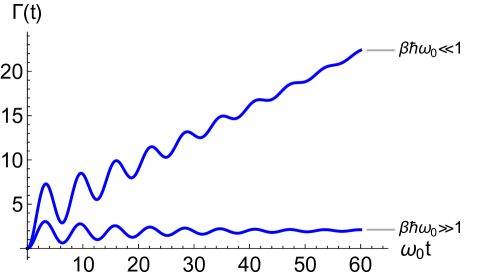
for the hyperbolic cotangent, with the so-called Matsubara frequencies, so that combining Eq. (43) and Eq. (44) we come to the expression
| (46) | |||||
with
| (47) |
and we consider the so-called underdamped limit in which . The behavior of this decoherence function as a function of time in the low and high temperature regime is plotted in Fig. 1
3.2 Non-Markovianity measure
In the considered dephasing model the reduced system dynamics is fixed by the transformation Eq. (42). This allows to evaluate the expression for relevant choices of given by , , and . We will consider an initial pair of system states given by two orthogonal pure states on the equator of the Bloch sphere. These pairs have the maximal initial distinguishability according to Eq. (3), and are mostly affected by the dynamics since they both initially have the maximum amount of coherence. It has further been shown that these pairs maximize the measure according to Eq. (29) for the case in which is the trace distance. We thus have
| (48) |
with projections on the pure orthogonal states
| (49) |
and we obtain for the trace distance
| (50) |
as well as for the distance given by the square root of the Jensen-Shannon divergence
| (51) |
The other quantifiers can be evaluated starting from the expression Eq. (10), exploiting the fact that for the case at hand . We finally obtain for the quantum skew divergence with
and for the Holevo skew divergence with
| (53) | |||||
3.2.1 Temperature and coupling strength dependence
We can now exploit the explicit time-dependent expressions for the decoherence function and for the different distinguishability quantifiers to investigate the temperature and coupling dependence of the non-Markovianity measure. Making reference to Eq. (28) and Eq. (50) we have
| (54) |
while considering Eq. (51) we obtain
| (55) | |||||
where the pairs denote the time windows in which the distinguishability quantifiers shows revivals. Similar but more cumbersome expressions can be written for and . All of these expressions provide monotonically increasing functions of , so that the pairs are determined by the time regions in which decreases, that can be determined numerically.
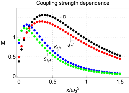
The behavior of these measures as a function of inverse temperature and coupling strength are plotted in Fig. 2 and Fig. 3 respectively. For the case of the temperature dependence they all show an increase of non-Markovianity for decreasing temperature. The two distances , have a very similar behavior and higher sensitivity with respect to the two divergences and . The Holevo skew divergence further shows a slightly stronger temperature dependence when compared with the quantum skew divergence . Investigating the coupling dependence strength all quantifiers point to a non-monotonic behavior of the measure, initially increasing and later vanishing for strong enough coupling. Also in this case the two distances , behave similarly and exhibit a higher sensitivity with respect to the two divergences and . Again the Holevo skew divergence features a slightly more marked coupling strength dependence with respect to the quantum skew divergence .
4 Conclusions
We have considered a general framework for the characterization of quantum non-Markovian dynamics, that is based on the behavior in time of the distinguishability between system states obtained starting from different initial conditions. The framework includes both distances and divergences. After a brief discussion of the physical motivation behind the approach, we have considered the behavior of distances and divergences in the study of a general physical model of decoherence. We investigate in particular the amount of non-Markovianity associated to the model in the dependence on physical parameters such as temperature and coupling strength. The behavior of two distances, namely trace distance and square root of the Jensen-Shannon divergence, is compared with the one of two divergences, namely Holevo and quantum skew divergence. It appears that the approach is robust with respect to the choice of quantifier, in that they all exhibit the same dependence on the physical parameters of the model. At the same time distances are more sensitive than divergences in their dependence on these parameters.
Acknowledgments
The work was partially supported by the Italian MIUR under PRIN 2022.
References
- [1] Á. Rivas, S. F. Huelga, and M. B. Plenio, Rep. Prog. Phys. 77, 094001 (2014). DOI: 10.1088/0034-4885/77/9/094001
- [2] H.-P. Breuer, E.-M. Laine, J. Piilo, and B. Vacchini, Rev. Mod. Phys. 88, 021002 (2016). DOI: 10.1103/RevModPhys.88.021002
- [3] I. de Vega and D. Alonso, Rev. Mod. Phys. 89, 015001 (2017). DOI: 10.1103/RevModPhys.89.015001
- [4] L. Li, M. J. Hall, and H. M. Wiseman, Phys. Rep. 759, 1 (2018). DOI: 10.1016/j.physrep.2018.07.001
- [5] S. Milz and K. Modi, PRX Quantum 2, 030201 (2021). DOI: 10.1103/PRXQuantum.2.030201
- [6] D. Chruściński, Phys. Rep. 992, 1 (2022). DOI: 10.1016/j.physrep.2022.09.003
- [7] H.-P. Breuer, E.-M. Laine, and J. Piilo, Phys. Rev. Lett. 103, 210401 (2009). DOI: 10.1103/PhysRevLett.103.210401
- [8] N. Megier, A. Smirne, and B. Vacchini, Phys. Rev. Lett. 127, 030401 (2021). DOI: 10.1103/PhysRevLett.127.030401
- [9] A. Smirne, N. Megier, and B. Vacchini, Phys. Rev. A 106, 012205 (2022). DOI: 10.1103/PhysRevA.106.012205
- [10] M. B. Ruskai, Rev. Math. Phys. 6, 1147 (1994). DOI: 10.1142/S0129055X94000407
- [11] K. M. R. Audenaert, e-print arXiv:1102.3041 (2011). DOI: 10.48550/arXiv.1102.3041
- [12] K. M. R. Audenaert, Telescopic Relative Entropy, in Theory of Quantum Computation, Communication, and Cryptography, edited by Bacon, Dave and Martin-Delgado, Miguel and Roetteler, Martin (Springer Berlin Heidelberg, Berlin, Heidelberg, 2014), pp. 39–52. DOI: 10.1007/978-3-642-54429-3_4
- [13] G. Lindblad, Commun. Math. Phys. 40, 147 (1975). DOI: 10.1007/BF01609396
- [14] S. Sra, Linear Algebra Appl. 616, 125 (2021). DOI: 10.1016/j.laa.2020.12.023
- [15] D. Virosztek, Adv. Math. 380, 107595 (2021). DOI: 10.1016/j.aim.2021.107595
- [16] E.-M. Laine, J. Piilo, and H.-P. Breuer, Phys. Rev. A 81, 062115 (2010). DOI: 10.1103/PhysRevA.81.062115
- [17] S. Campbell, M. Popovic, D. Tamascelli, and B. Vacchini, New J. Phys. 21, 053036 (2019). DOI: 10.1088/1367-2630/ab1ed6
- [18] G. M. Palma, K.-A. Suominen, and A. Ekert, Proc. Roy. Soc. A 452, 567 (1996). DOI: 10.1098/rspa.1996.0029
- [19] F. Settimo, H.-P. Breuer, and B. Vacchini, Phys. Rev. A 106, 042212 (2022). DOI: 10.1103/PhysRevA.106.042212
- [20] H.-P. Breuer and F. Petruccione, The Theory of Open Quantum Systems (Oxford University Press, Oxford, 2002)
- [21] U. Weiss, Quantum Dissipative Systems (World Scientific, Singapore, 1993)
- [22] G.-L. Ingold, Path Integrals and Their Application to Dissipative Quantum Systems, in Coherent Evolution in Noisy Environments, edited by Buchleitner, Andreas and Hornberger, Klaus (Springer, Berlin, 2002), Lect. Not. Phys., pp. 1–53. DOI: 10.1007/3-540-45855-7
- [23] A. Garg, J. N. Onuchic, and V. Ambegaokar, J. Chem. Phys. 83, 4491 (1985). DOI: 10.1063/1.449017
- [24] S. Mukamel, Principles of Nonlinear Optical Spectroscopy (Oxford University Press, 1995)
- [25] I. S. Gradshteyn and I. M. Ryzhik, Table of integrals, series and products (Academic Press, 1965)