Rate Function Modelling of Quantum Many-Body Adiabaticity

Abstract

The quantum adiabatic theorem is a fundamental result in quantum mechanics, which has a multitude of applications, both theoretical and practical. Here, we investigate the dynamics of adiabatic processes for interacting quantum many-body systems by analysing the properties of observable-free, intensive quantities. In particular, we study the rate function $f(T)$ in dependence of the ramp time $T$, which gives us a complete characterization of the many-body adiabatic fidelity as a function of $T$ and the strength of the parameter displacement $\Delta\lambda$. This allows us to control and define the notion of adiabaticity in many-body systems. Several key results in the literature regarding the interplay of the thermodynamic and the adiabatic limit are obtained as inferences from the properties of $f(T)$ in the large $T$ limit.

I Introduction

The quantum adiabatic theorem, which was first proposed by Born and Fock in 1928 [1], is a statement about the time evolution under slow parameter changes of a system initially prepared in one of the eigenstates. If we have a Hamiltonian $\mathcal{H}(\lambda(t))$ which is a function of a time dependent parameter $\lambda(t)$, then this defines a family of eigenstates $\ket{m_{\lambda}}$ for each value of $\lambda$. We start with an initial state $\ket{m_{\lambda_{i}}}$ corresponding to the parameter $\lambda_{i}$ and change the parameter to $\lambda_{f}$ over the ramp time $T$ to obtain the time evolved initial state $\ket{\Phi_{m}(T)}=\hat{\mathcal{U}}(T)\ket{m_{\lambda_{i}}}$. Then the theorem states that the quantum adiabatic fidelity, which is defined as

$$\mathcal{F}(T):=|\bra{m_{\lambda_{f}}}\ket{\Phi_{m}(T)}|^{2}\,,$$ (1)

for slow enough driving behaves as

$$\mathcal{F}(T)=1-\mathcal{O}(T^{-2})\,.$$ (2)

This means that for slow driving, the time evolved initial state points towards the corresponding final instantaneous eigenstate of $\mathcal{H}(\lambda(T))$, and that transitions to other energy levels are suppressed. The prerequisite for the application of the theorem is the absence of level crossings. The notion of ”slow enough” is quantified by the minimum of the energy gap $\Delta E$ along the trajectory, i.e., we require $T\gg(\text{min}(\Delta E))^{-1}$.

It is interesting to note that while the derivation of the theorem was introduced for single particle systems, the applications of the theorem range from relativistic field theories to condensed matter physics. The adiabatic theorem provides the conceptual foundation for Landau’s Fermi Liquid Theory [2] and the Gell-Mann Low [3] theorem. For these cases we assume that such an adiabatic process, in principle, is possible, even though the time scales, on which such slow changes take place, would extend to infinity. However, this is not a problem since here the theorem is used more as a formal device to connect the properties of the eigenstates of the unknown interacting systems with those of the well understood non-interacting ones.

It is on the practical side when it comes to adiabatic state preparation (and this can involve a multitude of fields ranging from cold atomic gases [4], adiabatic quantum computation [5, 6], topological charge pumping [7] etc.), that it becomes important to have a quantitative handle on the question, as to how slowly a process should be performed to remain within a prescribed bound of adiabaticity. In these situations we would like the many-body adiabatic fidelity $\mathcal{F}_{N}(T)$ for the entire system to deviate as little as possible from unity.

The goal of this paper is to study processes involving time dependent parameter changes in quantum many-body systems by analysing the properties of rate functions $f(T)$, which we define as

$$f(T):=-\lim_{N\rightarrow\infty}\frac{1}{N}\ln(\mathcal{F}_{N}(T))\,,$$ (3)

where $N$ is the number of particles. We study this quantity numerically for the XXZ model using exact diagonalization. In addition, we provide a field theoretical treatment in the Luttinger liquid phase of the XXZ chain. We will show how the knowledge of $f(T)$ can be used to obtain complete information about the many-body fidelity of the corresponding process for sufficiently large $N$ and arbitrary ramp times. For ramp duration $T=0$, $f(T=0)$ gives us the fidelity following a sudden quantum quench. In the large $T$ limit, $f(T)$ gives us the fidelity for an adiabatic process. More specifically, $f(T)$ will give us the corresponding value of $T$ for which a prescribed value of the many-body fidelity $\mathcal{F}_{N}(T)$ is achieved. We will also see how the qualitative properties of $f(T)$ change depending on the phases and the path through the phase diagram, which we choose for the ramp, and the implications it has for the approach to adiabaticity in terms of the dependence of adiabatic time scales with system size.

The remainder of the paper is structured as follows: In Sec. II we will go through several well known key results on the problem of adiabatic quantum many-body dynamics and alternative approaches to adiabaticity in many-body systems. In Sec. III we will motivate the definition of the rate function $f(T)$ by Eq. (3) and describe how it can be used to obtain time scales to achieve adiabaticity in many-body systems. In Sec. IV we will present the qualitative features of $f(T)$ and discuss about the various regimes with respect to $T$. In Sec. V we will study the rate functions for the XXZ spin chain in detail and see explicitly how the qualitative behaviour changes for processes within different phases followed by a summary and outlook in Sec. VI. In the appendices we go through the technical calculations.

II Properties of many-body adiabatic processes

Adiabatic processes in many-body settings have been studied in great detail, see, e.g., Refs. 8, 9, 10, 11, 12, 13. In this section, we highlight the most relevant results (we use in the following the notation applied in this paper).

Lychkovskiy et al. [10] present a lower bound on the ramp time $T$ (inverse of the driving speed $\Gamma_{N}$ in their notation) for an adiabatic process with very modest inputs in terms of the scaling properties of the the many-body ground states. These scaling properties are characterised by parameters, which are denoted as $C_{N}$ and $\delta V_{N}$, and are introduced as follows:

$C_{N}$ quantifies the strength of the orthogonality catastrophe. It is obtained by exploring the dependence of many-body overlaps for different values of some system parameter $\lambda$ in the large $N$ limit,

$$\mathcal{C}(\lambda)\equiv|\bra{\Phi_{\lambda}}\ket{\Phi_{0}}|^{2}=\exp(-C_{N}\lambda^{2}).$$ (4)

For example, for impurity models $C_{N}\sim\ln(N)$, while for global parameter changes (i.e., the situations considered in this paper) one obtains $C_{N}\sim N$.

$\delta V_{N}\equiv\sqrt{\langle\hat{V}^{2}\rangle_{0}-\langle\hat{V}\rangle_{0}^{2}}$ is the uncertainty in the driving potential with respect to the ground state where $\left.\hat{V}\equiv\frac{\partial\hat{H}}{\partial\lambda}\right|_{\lambda=0}$. From these one obtains bounds for the ramp time needed to observe adiabatic behavior for the $N$ body state, namely

$$T\geq\frac{2C_{N}}{\delta V_{N}}\,.$$ (5)

For example, for a gapped system where we perform a global parameter change adiabatically, we have $\delta V_{N}\sim\sqrt{N}$ and $C_{N}\sim N$, and therefore

$$T\geq 2\sqrt{N}\,.$$ (6)

In [12], Polkovnikov focuses on adiabatic processes in the vicinity of quantum critical points and relates the density of excitations $n_{\rm ex}$ (number of excited states upon the total number of states) to the critical exponents $\nu,z$, the ramp time $T$ (again the inverse of the driving speed $\delta$ in their notation), and the dimensionality $d$ as

$$n_{\text{ex}}\propto T^{-d\nu/(1+z\nu)}\,.$$ (7)

For the case of the one dimensional transverse field Ising model, for which we have $\nu=d=z=1$, we get

$$n_{\text{ex}}\propto\frac{1}{\sqrt{T}}\,,$$ (8)

which matches the result of Ref. 9 derived using the Landau-Zener formula.

In another work [8], De Grandi and Polkovnikov find that the density of excitations of noninteracting quasiparticles within a gapless phase having dispersion relation $\epsilon_{k}=c(\lambda)k^{z}$ turns out to be

$$n_{\text{ex}}\propto T^{-d/z}\,.$$ (9)

For a Tomonaga-Luttinger liquid, $d=z=1$ and we find $n_{\text{ex}}\propto 1/T$.

Here we would like to point out that for the case of global parameter changes, (which means $C_{N}\sim N$) all of these results in different cases emerge naturally as properties of the rate function $f(T)$ discussed in this paper, in the large $T$ limit. For non-interacting gapped systems we will show $f(T)$ to be directly related to the transition probabilities of individual subsystems whereas for gapless systems or critical points, $f(T)$ measures the density of quasiparticle excitations for any given ramping time $T$.

A completely separate direction is taken by Bachmann et al. [14] who base their analysis on observable dependent quantities. They work with a different definition of adiabaticity, which they define as the convergence of the expectation values of some local operator $\hat{O}$, with respect to the time evolved initial state $|\psi(s)\rangle$, and the instantaneous eigenstate at the final parameter value $|\Omega_{s}\rangle$ ($C$ is some non-universal constant independent of the system size and $\varepsilon$ is some small parameter)

$$\left|\langle\psi(s)|\hat{O}|\psi(s)\rangle-\langle\Omega_{s}|\hat{O}|\Omega_{s}\rangle\right|\leq C\varepsilon\,.$$ (10)

They show that the adiabatic condition so defined becomes independent of the system size. In our work, in contrast, we stick to analysing the behavior of the wave-function overlaps by studying the rate function, which we introduce in the next section and in this way avoid any observable specific discussions.

III Many-Body Rate Function $f(T)$

III.1 Definition

We start with a many-body Hamiltonian with a time dependent parameter $\mathcal{H}(\lambda(t))$. Each value of $\lambda$ defines a set of instantaneous eigenstates $\ket{n_{\lambda}}$. We choose the initial and final parameters $\lambda_{i}$ and $\lambda_{f}$ respectively and also the ramping time $T$ which decides the duration of the process. We choose a simple linear ramp,

$$\lambda(t)=\lambda_{i}+\frac{t}{T}(\lambda_{f}-\lambda_{i}),$$ (11)

where time $t\in[0,T]$.

At $t=0$, we are in the ground state of $\lambda_{i}$, which is $\ket{0_{\lambda_{i}}}$. Then we perform the unitary time evolution $\hat{\mathcal{U}}(T)$ generated by $\mathcal{H}(\lambda(t))$, and ask how well does the final time evolved state vector point towards the ground state corresponding to the final parameter value $\lambda_{f}$.

According to the previous discussion, the many-body fidelity for a system with $N$ particles is given by $\mathcal{F}_{N}(T)=|\bra{0_{\lambda_{f}}}\hat{\mathcal{U}}(T)\ket{0_{\lambda_{i}}}|^{2}$. We posit the following ansatz

$$\mathcal{F}_{N}(T)\equiv\exp(-N\cdot f_{N}(T,\lambda_{i},\lambda_{f}))\,,$$ (12)

from which we obtain ($\lambda_{i},\lambda_{f}$ removed for clarity of notation)

$$f_{N}(T)=-\frac{1}{N}\ln\left(\mathcal{F}_{N}(T)\right)\,.$$ (13)

$f_{N}(T)$ is the quantity that can be obtained via numerics. The definition becomes useful since $f_{N}(T)$ has a well defined thermodynamic limit for the global parameter quenches that we discuss in this paper. We define this limit as the rate function

$$f(T)\equiv\lim_{N\rightarrow\infty}f_{N}(T)\,.$$ (14)

If $f_{N}(T)$ converges sufficiently quickly then for large $N$ we can evaluate $\mathcal{F}_{N}(T)$ using

$$\mathcal{F}_{N}(T)=\exp(-N\cdot f(T))\,.$$ (15)

In practice what this means is that the rate function can be used to obtain all the information about the many-body overlaps for large $N$ and arbitrary ramp times $T$.

We follow the discussion in Ref. 14 and motivate the ansatz in Eq. (12) heuristically by looking at many-body product states: for example, for two quantum spin-1/2 particles, whose directions are off by a small angle $\theta$, their direct overlap would be

$$|\bra{\psi+\theta}\ket{\psi}|^{2}=1-\mathcal{O}(\theta)\approx\exp(-\mathcal{O}(\theta))\,.$$ (16)

If we have $N$ such pairs of decoupled spins, due to the tensor product structure, the overlap of the entire quantum state is just the product of individual overlaps:

$$|\bra{\psi+\theta}\ket{\psi}_{N}|^{2}=\prod_{i}\exp(-\mathcal{O}(\theta))=\exp(-N\mathcal{O}(\theta))\,.$$ (17)

We point out that the equation above works only for global parameter changes (i.e., all the angles $\theta$ in the entire many-body system are changed). For local perturbations, the situation can be very different, and the $N$ dependence of the direct overlap (see Eq. (17)) changes its form. For example, in Anderson’s original work on the orthogonality catastrophe [15], he studied the effect of impurities in metallic systems and obtained overlaps, which decay algebraically with system size as $N^{-\epsilon}$, where $\epsilon$ quantifies the strength of the impurity.

Next, we want to incorporate the explicit time evolution in the expressions. In the aforementioned case this corresponds to some physical process, which aligns the spins of state $\ket{\psi}$ with those of $\ket{\psi+\theta}$, where it takes a time $T$ to change the angle by $\theta$. Here, we simply absorb the $T$-dependence in the exponential,

$$|\bra{\psi+\theta}\mathcal{U}(T)\ket{\psi}_{N}|^{2}=\exp(-N\mathcal{O}(\theta,T))\,.$$ (18)

For this process, the rate function will be

$$f(T)=\mathcal{O}(\theta,T)\,.$$ (19)

Working in the quantum many-body regime presents us with an interesting complication, which is the presence of a multitude of quantum phases and critical points in the parameter space. Critical points or gapless phases imply that the energy gaps vanish in the thermodynamic limit. The adiabatic dynamics sensitively depends on the behaviour of energy gaps and consequently on whether the initial and final parameters lie entirely within the same phase or have a critical point in between them. As we will see, the specifics of the process in the parameter space will lead to qualitative changes in the behaviour of the properties of $f(T)$.

$f(T)$ has a nice physical interpretation as it is a non-negative, intensive quantity. Therefore, it is well defined in the thermodynamic limit and provides a quantitative measure of deviation from adiabaticity for the entire range of ramping times, for small $T$ (fast ramps) to large $T$ (adiabatic limit), independent of the system size. Knowledge of $f(T)$ can be used to quantitatively evaluate the fidelity for any system size $N$ for the corresponding physical process (from $\lambda_{i}$ to $\lambda_{f}$). On the theoretical side, analysing the properties of $f(T)$ in the large $T$ limit, along with the ansatz of our many-body overlap in Eq. (12), allows us to obtain the results we discussed in Sec. II.

III.2 $f(T)$ and Adiabatic Time scale $T_{N}$

The rate function provides us with a direct relationship between the notion of an adiabatic time scale $T_{N}$, the system size $N$ and the parameter displacement $\Delta\lambda=\lambda_{f}-\lambda_{i}$.

In the examples we look at, we find that for large ramp time $T$, $f(T)$ shows an algebraic decay in $T$ and is quadratically dependent on $\Delta\lambda$ (for details see Appendix[A]),

$$f(T)\propto(\Delta\lambda)^{2}/T^{\alpha}.$$ (20)

With this relation, we have

$$\mathcal{F}_{N}(T)=\exp(-\gamma\frac{(\Delta\lambda)^{2}N}{T^{\alpha}}),$$ (21)

where $\gamma$ and $\alpha$ are non-universal constants.

If at the end of an adiabatic process, we want a prescribed many-body fidelity quantified by some small parameter $\delta$

$$\mathcal{F}_{N}(T)=1-\delta=\exp(-\gamma\frac{(\Delta\lambda)^{2}N}{T^{\alpha}})\,,$$ (22)

then we immediately obtain the notion of an adiabatic timescale $T_{N}$, which gives us the time that it takes to make the entire $N$-body state evolve adiabatically, as

$$T_{N}\propto(N)^{1/\alpha}(\Delta\lambda)^{2/\alpha}\,.$$ (23)

This quantifies the time it takes to get the entire many-body fidelity $\mathcal{F}_{N}(T)$ close to unity. However, while Eq. (23) is always valid for gapped phases, it is not applicable in general, because we need to introduce a crossover time-scale $T_{C}$, bridging the fast ramps and the adiabatic regime as discussed in detail in Sec. IV.2.

III.3 $f(T)$ for Non-Interacting Gapped Systems

We make use of the Born-Fock result, to find the $f(T)$ for gapped non-interacting system. For an individual gapped subsystem, the Born-Fock result shows that for $T$ much larger than the minimum of the inverse gap size, the following relation holds

$$\mathcal{F}(T)=|\bra{0_{\lambda_{f}}}\hat{\mathcal{U}}(T)\ket{0_{\lambda_{i}}}|^{2}=1-\mathcal{O}(T^{-2}).$$ (24)

If we have a tensor product of non-interacting gapped systems (the energy gaps need not be the same) the many-body fidelity is simply the product of individual fidelities

$$\begin{split}\mathcal{F}_{N}(T)=&\prod_{k=1}^{N}|\bra{0^{k}_{\lambda_{f}}}\hat{\mathcal{U}}(T)\ket{0^{k}_{\lambda_{i}}}|^{2}\\ =&\prod_{k=1}^{N}(1-\mathcal{O}_{k}(T^{-2}))\approx\prod_{k=1}^{N}\exp(-\mathcal{O}_{k}(T^{-2})),\end{split}$$ (25)

where $k$ is just an index for individual subsystem.

The product of exponentials becomes a sum of the exponents and gives us

$$\mathcal{F}_{N}(T)=\exp(-N\cdot\frac{1}{N}\sum_{k}\mathcal{O}_{k}(T^{-2})),$$ (26)

from which we can immediately write down $f(T)$ as

$$f(T)=\frac{1}{N}\sum_{k}\mathcal{O}_{k}(T^{-2})\propto\frac{1}{T^{2}}.$$ (27)

This is the exact algebraic decay exponent we find for $f(T)$ in the $T>T_{C}$ regime even for interacting systems and its direct relation to the Born Fock result is what motivates us to call this the many-body adiabatic regime.

Using Eq. (23), we immediately find

$$T_{N}\propto\sqrt{N},$$ (28)

which is the same result for gapped systems in Eq. (6) derived by Lychkovskiy et.al. [10].

IV General Properties of $f(T)$

IV.1 Quench and Many-Body Adiabatic regimes

The general shape of the rate function $f(T)$ which we will see throughout is shown in Fig.[1].

We refer to the red region as the fast ramp regime because here the ramping times are short compared to the inverse of the energy gaps, which means there is a rapid change of the system parameter. The decay is again algebraic but the decay exponent depends strongly on the specific system for which the process is being performed.

We refer to the green region as the many-body adiabatic regime because in this region, ignoring the oscillations, $f(T)$ decays as $1/T^{2}$. We saw earlier in Sec. III.3, that it is partially in sync with the Born and Fock notion of adiabaticity. This is because even though for large enough $N$, the fidelity $\mathcal{F}_{N}(T)$ itself might be small, the decay exponent $\alpha=2$ is directly related to the Born-Fock result as seen in Eq. (27). We point out that our notion of many-body adiabatic regime for $f(T)$ is different from the one introduced by Born and Fock where they defined adiabaticty as the vanishing deviation of fidelity from unity. The exponential size of the many-body Hilbert space forces us to introduce an additional adiabatic time scale $T_{N}$ which scales with system size as we saw in Eq. (23).

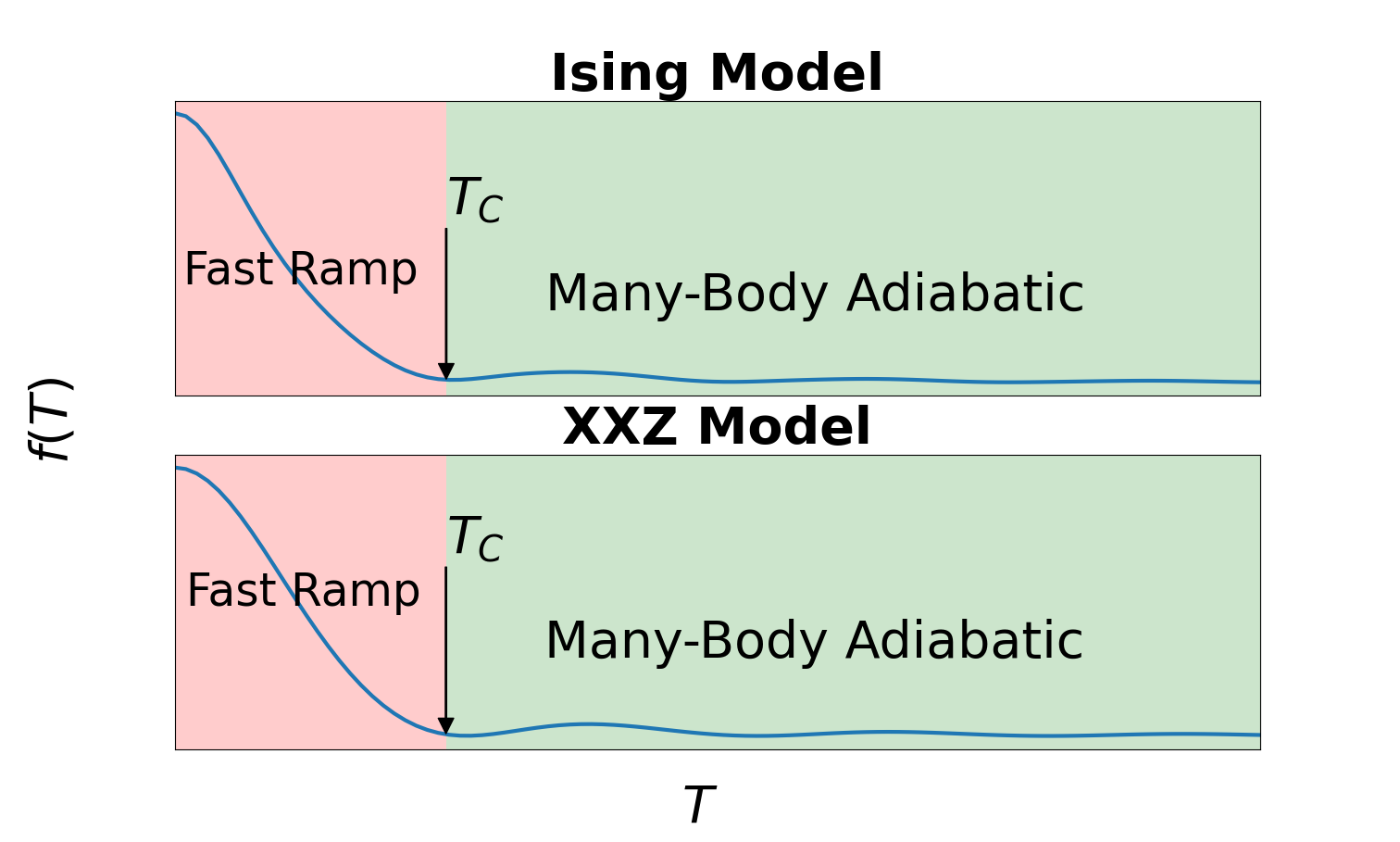
Figure 1: General behavior of $f(T)$. Two regimes can be identified: for fast ramps ($T<T_{c}$, indicated in red), one obtains a monotonic decay of $f(T)$. For slow ramps ($T>T_{c}$, indicated in green), one is in the many-body adiabatic regime, with an oscillatory $1/T^{2}$ decay of $f(T)$. The crossover time $T_{C}$ (which depends on the inverse of the energy gaps) separates the two regimes; this generic behavior is found to be independent of the physical system and the choice of parameters.

IV.2 Crossover time $T_{C}$

We call $T_{C}$ the crossover time bridging the fast ramp and the many-body adiabatic regimes. It is expected to depend on the minimum of the energy gap during the process. For a process remaining within a gapped phase, the energy gaps are (up to typically comparably small finite-size effects) independent of the system size, and hence we do not expect a $N$-dependence of $T_{C}$.

However, if a many-body system possesses a gapless critical point along the process (e.g., in the Ising model) or a gapless region (like in the XY phase of the XXZ model), then the energy gaps are (to leading order) inversely proportional to the system size, and therefore $T_{C}\propto N$. As a consequence of this, in the thermodynamic limit $T_{C}$ runs off to infinity and $f(T)$ only shows the fast ramp regime. Now the crucial point is that for finite $N$, even when the ramps encounter gapless phases or critical points, as soon as $T$ goes beyond $T_{C}$, we find that $f(T)$ changes its behavior to a $1/T^{2}$ oscillatory decay and we find ourselves in the many-body adiabatic regime.

Let us consider the consequences of these aspects for the adiabatic time scale $T_{N}$ for three specific cases.

• For ramps across gapped phases we will see in Sec. V.1.2 that $\alpha=2$. $T_{C}$ is independent of the system size and Eq.(23) implies $T_{N}\propto\sqrt{N}$.

• For ramps across the Luttinger Liquid phase of any system, we will see in Sec. V.2 that $\alpha=1$. Since we are in a gapless phase we also have $T_{C}\propto N$ and $T_{N}\propto N$.

• However, for ramps across the Ising critical point, we will find in Sec. V.2 that $\alpha=0.5$. This implies that $T_{N}\propto N^{2}$. This conclusion would be valid if $f(T)\propto 1/\sqrt{T}$ throughout the large $T$ limit. However, as argued earlier, what happens is that for any given $N$ we still have $T_{C}\propto N$ and as soon as $T\sim T_{C}\sim N$, $f(T)$ changes its qualitative behavior from $1/\sqrt{T}$ to $1/T^{2}$. The implication for this setup is that the result of $T_{N}\propto N^{2}$ is an overestimate and $T_{N}\propto N$ is adequate.

V $f(T)$ for the XXZ model

In this paper we focus on the 1D XXZ model. It has a rich phase diagram which allows us to look at various regimes and make a variety of inferences. The particular Hamiltonian we work with is

$$\hat{H}(t)=-J_{xy}\sum_{i=1}^{N}\left(S^{x}_{i}S^{x}_{i+1}+S^{y}_{i}S^{y}_{i+1}\right)-J_{z}(t)\sum_{i=1}^{N}S^{z}_{i}S^{z}_{i+1}.$$ (29)

We set $J_{xy}=1$ and ramp the time dependent parameter $J_{z}(t)$. Within the gapped anti-ferromagnetic ($J_{z}(t)<-1.0$) and ferromagnetic ($J_{z}(t)>1.0$) phases, we make use of exact diagonalization and use the python package QuSpin [16, 17] which will allow us to treat system sizes $N\sim\mathcal{O}(20)$. In the XY phase ($|J_{z}(t)|<1.0$) we study the system by mapping it to a Luttinger Liquid. In this way, we can exactly solve systems with $N\sim\mathcal{O}(1000)$ or larger and study its properties analytically by making use of adiabatic perturbation theory.

V.1 Within Gapped Phases

V.1.1 Within the FM Phase ($J_{z}(t)>1.0$)

The ferromagnetic ground state is simply all spins pointing in the same direction with the spin-z magnetization $\langle\sigma_{z}\rangle=\pm 1$. There is only one single state within the chosen magnetization sector, and since the $H_{\text{XXZ}}$ conserves magnetization symmetry, there is no possibility for the system to make a transition to any other state no matter how fast or slow the driving for $J_{z}(t)$ is. Since $f(T)$ measures transition probabilities, this means that for driving within the FM phase we obtain $f(T)=0$.

V.1.2 Deep within the AFM Phase ($J_{z}(t)\ll-1.0$)

The AFM phase presents us with two degenerate ground-states (the two Néel states). We restrict ourselves to the positive parity subsector by choosing the symmetric combination of the two degenerate Néel states as our initial ground state. In this phase $f(T)$ shows the exact same qualitative behaviour as shown earlier in Fig.[1], and we see the demarcation into fast ramp and many-body adiabatic regimes in Fig.[2].

Eq. (27) insinuates that even for this interacting many-body gapped phase the behavior should follow $f(T)\sim 1/T^{2}$. In the inset of Fig. [2] we test this, as shown by the solid line, which is intended as guide to the eye. The data oscillates around this line, but otherwise it follows this behavior well. This implies that in this regime

$$f(T)\propto\frac{1}{T^{2}}\,.$$ (30)

The oscillatory behavior of $f(T)$ is highly non-universal. We can see the oscillations appearing even in the extremely simple problem of a collection of non-interacting precessing spins as done in Appendix[B]. In Fig.[2] we see that the oscillations also depend on $N$. These are entirely due to finite size effects.

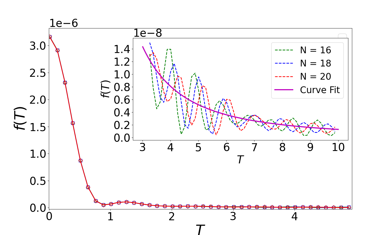
Figure 2: $f(T)$ for ramps deep within the AFM phase of the XXZ spin chain. $J_{z}(t)$ ramps from $-7.4$ to $-7.6$. $T$ is measured in units of $1/J_{xy}$ . The inset is a zoom into the large-$T$ region and shows the finite-size data in comparison to a curve fit of the form $a/T^{2}$. As an be seen, the difference between the results for different $N$ is very small, so that they cannot be distinguished in the main plot.

Due to strong finite size effects, the system sizes amenable to exact diagonalization are too small to study the properties of $f(T)$ for ramps close to or across the BKT critical point $J_{z}=-1.0$. This is discussed in more detail in App. E.

V.2 Within the Gapless XY Phase ($|J_{z}(t)|<1.0$)

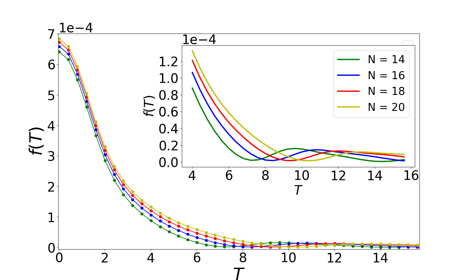
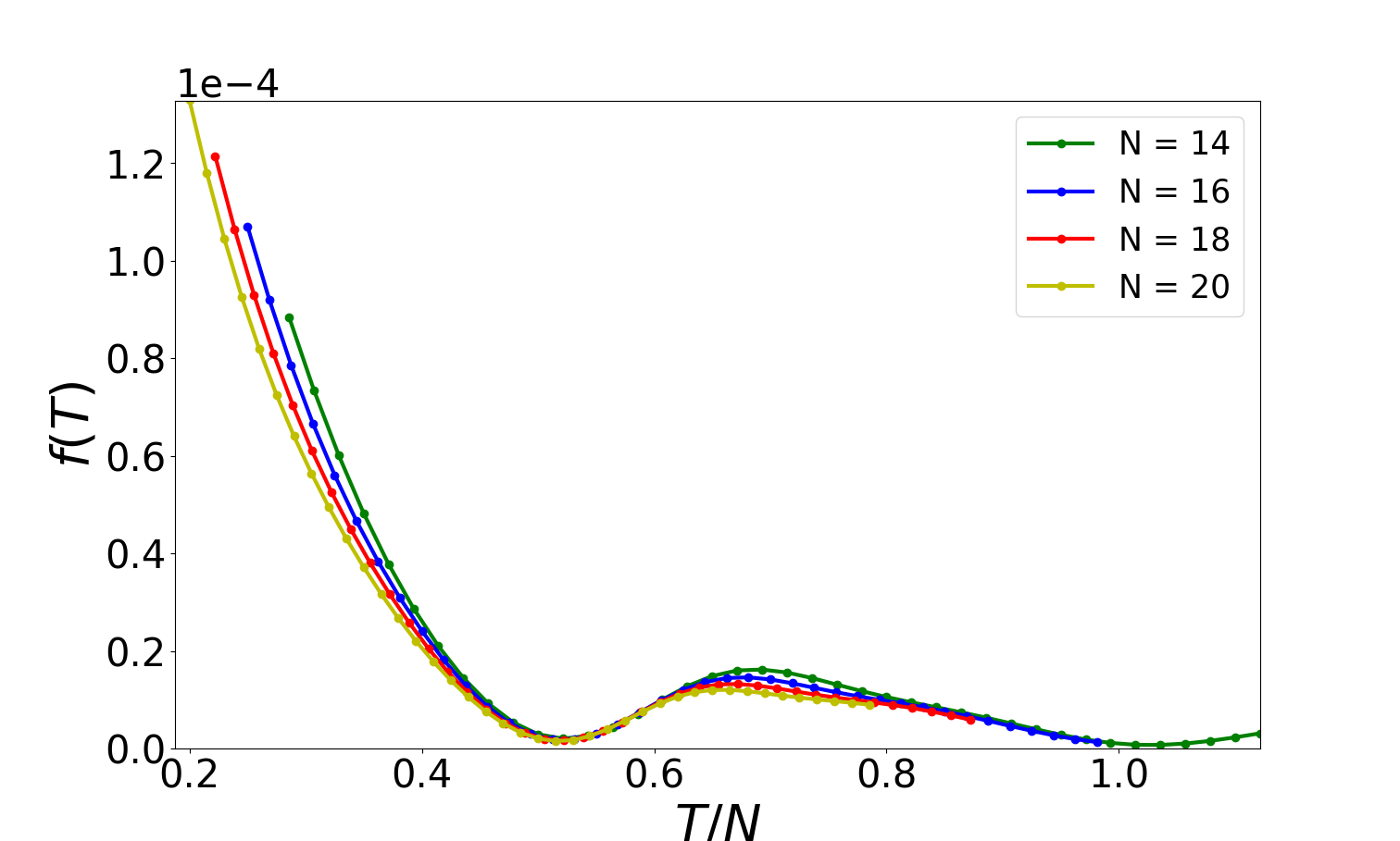
Figure 3: a) Ramps within the XY phase for small $N$. $J_{z}(t)$ ramps from $-0.1$ to $0.1$. In the inset plot (dots removed for clarity) we see that $T_{C}$ is increasing with $N$. We also see the change in algebraic decay from $1/T$ to $1/T^{2}$ as $T$ increases.
b) Rescaling the x-axis shows that $T_{C}/N$ is constant for various system sizes.

First, we notice in this phase the strong finite size effects on the behaviour of $f(T)$. Specifically on the dependence of $T_{C}$ on the system size. For finite size gapless systems, $T_{C}\propto N$ (inverse of the gap size). For any fixed $N$, when $T>T_{C}$, which is the many-body adiabatic regime, $f(T)$ again decays as $1/T^{2}$. In the thermodynamic limit, $T_{C}$ will be pushed to infinity and we will see that in the fast ramp regime, $f(T)\propto 1/T$. This is obtained analytically by analysing $f(T)$ for Luttinger Liquids, as discussed in the next section which will also show us that $f(T)$ has a well defined thermodynamic limit even for a gapless system.

V.2.1 $f(T)$ for Luttinger Liquids

To study the system in the thermodynamic limit we map the XXZ model in the XY phase to the Luttinger Liquid (LL) which is an exactly solvable effective theory and evaluate $f(T)$ for this system instead.

After matching the XXZ model parameters to that of the LL [18] by setting $\omega=J_{xy}$ and $\Delta(t)=\frac{2}{\pi}J_{z}(t)$, we end up with the following Hamiltonian [19]($b_{q},b^{\dagger}_{q}$ are bosonic creation and annihilation operators for a particular $q$ mode):

$$\begin{split}H_{\text{TLL}}&=\sum_{q}H_{q}(t)\\ &=\sum_{q}|q|\left((\omega+\Delta(t))b^{\dagger}_{q}b_{q}+\frac{\Delta(t)}{2}\left[b_{q}b_{-q}+b^{\dagger}_{q}b^{\dagger}_{-q}\right]\right)\,.\end{split}$$ (31)

We introduce $\alpha_{q}=\frac{1}{\sqrt{2}}(b_{q}+b_{-q})$ and $\beta_{q}=\frac{i}{\sqrt{2}}(b_{q}-b_{-q})$ and re-express the previous Hamiltonian in terms of these new operators to obtain

$$H_{\text{TLL}}=\sum_{q>0}H_{q}(t)+H_{-q}(t)=\sum_{q>0}H_{q}^{\alpha}(t)+H_{q}^{\beta}(t)\,,$$ (32)

where ($a=\alpha,\beta$ labels the particle)

$$H^{a}_{q}(t)=q\left((\omega+\Delta(t))a^{\dagger}_{q}a_{q}+\frac{\Delta(t)}{2}\left[(a_{q})^{2}+(a_{q}^{\dagger})^{2}\right]\right)\,.$$ (33)

Since $[\alpha_{q},\beta_{q}^{\dagger}]=0$ for all $q$, the Hilbert space is bifurcated into two sectors (the individual $q$ modes of $\alpha$ and $\beta$ particles).

This problem is well suited for using the Adiabatic Perturbation theory [20, 8] discussed in Appendix[A], because for each instant of time $t$, we can diagonalize the Hamiltonian, write down the eigenstates and the energy spectrum and define an instantaneous eigenbasis which is non-degenerate (see Appendix[C]).

Since the system is non-interacting in $q$, for large $T$ $f(T)$ can be written as

$$f(T)=\frac{1}{N}\sum_{q}\mathcal{O}_{q}(T)\,,$$ (34)

where $\mathcal{O}_{q}(T)$ is the transition probability for an individual $q$ mode. This also tells us that our ansatz for $\mathcal{F}_{N}(T)$ is suitable even for gapless systems because it gives us a well defined $f(T)$.

Here we repeat the important fact that $\mathcal{O}(T)\sim 1/T^{2}$ is true only when $T$ is much larger than the inverse energy gap size for all individual subsystems. For a particular $q$ mode of the LL, the gap vanishes for small enough $q$ and as a consequence, for any given $T$, there is a collection of modes ranging from $0$ to $q_{c}(T)$, where $q_{c}(T)$ is the upper bound on the number of modes which are strongly excited during the process. Strong excitations correspond to large transition probabilities which means that the behavior of $f(T)$ is dominated by these strongly excited modes

$$f(T)=\frac{1}{N}\sum_{q}\mathcal{O}_{q}(T)\approx\frac{1}{N}\sum_{q=0}^{q_{c}(T)}\mathcal{O}_{q}(T)\,.$$ (35)

The density of excitations for any given ramp time $T$ is given by [8]

$$q_{c}(T)\propto 1/T\,.$$ (36)

This leads to

$$f(T)\approx\frac{1}{N}\sum_{q=0}^{q_{c}(T)}\mathcal{O}_{q}(T)\approx\int_{0}^{q_{c}(T)}\mathcal{O}_{q}(T)\;dq\,.$$ (37)

Re-expressing in terms of a rescaled variable $Tq=q^{\prime}$, ($\mathcal{O}_{q}(T)$ becomes independent of $T$ when expressed in terms of $q^{\prime}$. See Eq.(50)) gives us

$$f(T)\propto 1/T\,.$$ (38)

The result is confirmed in Fig.[4], which is evaluated using adiabatic perturbation theory without making the approximation in Eq. (35). This example is emblematic of the more general result that for processes across gapless regions or points, $f(T)$ is a direct measure of the density of quasi-particle excitations. What this implies is that $f(T)$ has the same dependence on $T$ as the density of excitations $n_{\text{ex}}(T)$.

The derivation of Eq. (38) was a direct result of the approximation made in Eq. (35), which has a very general character and can be applied whenever we have the knowledge of $n_{\text{ex}}(T)$ vs $T$. The values of $\alpha$ for $n_{\text{ex}}(T)\propto 1/T^{\alpha}$ have been evaluated for various critical points (for example for the Ising critical point $\alpha=1/2$) and can be found in Ref. 13 . For these cases, we will also have $f(T)\propto 1/T^{\alpha}$.

Figure 4: $f(T)$ for the Luttinger Liquid obtained by adiabatic perturbation theory. $J_{z}(t)$ ramps from $-0.1$ to $0.1$. The curve fit is carried out by $a/T$ where $a$ is the curve fitting parameter. This validates the result obtained in Eq. (38).

VI Summary and Outlook

In this paper we investigated the physics of time dependent parameter changes in quantum many-body systems by analysing the properties of rate functions $f(T)$. We expect our findings to be relevant for various realizations, like cold atomic gases [4], adiabatic quantum computation [5], many-body topological charge pumping [21], where it is possible to write down simple model Hamiltonians that describe the system at hand, and which allow for the evaluation of $f(T)$.

In Sec. III.1, we started our analysis by noting that for global parameter changes, the many-body fidelity between any two quantum states decays exponentially with system size $N$. This implies that increasing the ramp time $T$ for any time-dependent parameter change would bring the relevant many-body fidelity closer and closer to unity (which is the adiabatic limit). In contrast, for any given $T$, increasing $N$ will diminish these overlaps to zero.

To study this competition between the thermodynamic and the adiabatic limits systematically, we first motivated an ansatz for the fidelity of a many-body system experiencing a time dependent parameter change and separated the $T$ and the $N$ dependent parts. This allowed us to define the rate function $f(T)$ for the process which we showed to be an intensive quantity that does not depend on $N$. We showed how the knowledge of $f(T)$ provides us with the many-body fidelity for any $N$ for the corresponding process both in the small $T$ (quench) and the large $T$ (adiabatic) limit. We showed how the knowledge of $f(T)$ along with our ansatz of many-body fidelity provided us with the notion of an adiabatic time scale $T_{N}$ which depends on $N$ and makes sure that on these time scales the entire many-body fidelity evolves close to unity.

In Sec. IV.1, we saw that $f(T)$ vs $T$ possesses two qualitatively distinct regions. For $T<T_{C}$ we are in the fast ramp regime, where $f(T)$ has a monotonic algebraic decay in $T$. For $T>T_{C}$ we are in the many-body adiabatic regime, which has an oscillatory algebraic decay in $T$ with a different decay exponent. $T_{C}$ is the ramp time that bridges these two regimes. We argued that $T_{C}$ is controlled by the minimum of the energy gap during the process. As a consequence of this, we found that for ramps within gapped phases, $T_{C}$ is independent of $N$ whereas for ramps within gapless phases or across quantum critical points, $T_{C}$ becomes proportional to $N$.

In Sec. III.3, we evaluated $f(T)$ for the simple case of a collection of gapped non-interacting systems. We found that for this case, for $T$ larger than $T_{C}$, $f(T)$ is just the average of the transition probabilities of the individual sub-systems and that the algebraic decay exponent for $f(T)$ is 2.

In Sec. V we tested our ideas by evaluating $f(T)$ for the XXZ model using exact diagonalization and bosonization. We found that for processes within the gapped anti-ferromagnetic phase, the algebraic decay exponent for $f(T)$ was again $2$, and that $f(T)$ quickly reached a well defined thermodynamic limit even for relatively small system sizes. Exact diagonalization for processes in the XY phase showed us that $T_{C}\propto N$. To study the properties of $f(T)$ in the thermodynamic limit in this phase we studied the Luttinger liquid theory for this system. We found that the algebraic decay exponent for this case is $1$. We derived this decay exponent by first pointing out the direct relation between $f(T)$, and the density of excitations for this process, and then relating the excitation density to the ramp time $T$. The idea of relating $f(T)$ to the density of quasi-particle excitations is extremely general and is valid for other models which describe the physics in the vicinity of quantum critical points as well.

It will be interesting to investigate for new qualitative features emerging if we study the behaviour of $f(T)$ for systems that do not allow for a quasi-particle description for e.g., the SYK model [22].

VII Acknowledgements

We thank Marin Bukov for insightful discussions and Rishabh Jha for helpful comments on an earlier version of the manuscript. We acknowledge financial support by the Deutsche Forschungsgemeinschaft (DFG, German Research Foundation) - 217133147/SFB 1073, projects B03 and B07.

Appendix A Adiabatic Perturbation Theory

Here we go through the steps to perform Adiabatic perturbation theory [8, 20].

We consider the time-dependent Hamiltonian and we say that for each instant of time $t$, it defines an orthonormal basis set,

$$\hat{H}(t)\ket{\psi_{n}(t)}=E_{n}(t)\,,\ket{\psi_{n}(t)}$$ (39)

where for each $t$ we have

$$\bra{\psi_{m}(t)}\ket{\psi_{n}(t)}=\delta_{m,n}\,.$$ (40)

We can expand any quantum state at time $t$ in terms of these instantaneous eigenstates,

$$\ket{\Psi(t)}=\sum_{n}c_{n}(t)\ket{\psi_{n}(t)}\exp(-i\int_{0}^{t}dt^{\prime}E_{n}(t^{\prime}))\,.$$ (41)

If the initial state is some eigenstate of $\hat{H}(t=0)$ labelled by some index $m$, that just implies

$$\ket{\Psi(t=0)}=\ket{\psi_{m}(t=0)}\implies c_{n}(t=0)=\delta_{m,n}\,.$$ (42)

The advantage of this framework is that we only need to worry about the behaviour of $c_{n}(t)$, provided all other quantities ($\ket{\psi_{n}(t)},E_{n}(t)$) in principle are known. This is the case for all Bogoliubov type models, be it fermionic (like Ising model, Kitaev honeycomb model, XY model etc) or bosonic (Luttinger liquids).

The adiabatic condition (for the initial state $\ket{\psi_{m}(t=0)}$) can then be framed as

$$\begin{split}\lim_{T\rightarrow\infty}|\bra{\psi_{m}(T)}\ket{\Psi(T)}|^{2}&=|c_{m}(T)|^{2}\\ &=1-\mathcal{O}_{m}(T)\rightarrow 1\,,\end{split}$$ (43)

where (due to the normalization constraint on $\ket{\Psi(T)}$)

$$\mathcal{O}_{m}(T)=\sum_{n\neq m}|c_{n}(T)|^{2}$$ (44)

is the probability for the initial state to make a transition to any other state during the time evolution. The differential equations for the coefficients $c_{l}(t)$ are

$$\begin{split}\dot{c}_{l}(t)=&-c_{l}(t)\langle\psi_{l}(t)\mid\dot{\psi}_{l}(t)\rangle\\ &-\sum_{n\neq l}c_{n}(t)\frac{\langle\psi_{l}(t)|\dot{H}|\psi_{n}(t)\rangle}{E_{n}(t)-E_{l}(t)}e^{-i\int_{0}^{t}\left[E_{n}\left(t^{\prime}\right)-E_{l}\left(t^{\prime}\right)\right]dt^{\prime}},\end{split}$$ (45)

where $\ket{\dot{\psi}(t)}=\frac{\partial}{\partial t}\ket{\psi(t)}$. The above differential equations can be solved numerically quite easily for quadratic systems.

The first term of Eq. (45) can safely be ignored because we can always choose a gauge

$$\ket{\psi(t)}=e^{i\theta(t)}\ket{\phi(t)}$$ (46)

by choosing $\theta(t)$ such that

$$\bra{\psi(t)}\ket{\dot{\psi}(t)}=i\dot{\theta}(t)+\bra{\phi(t)}\ket{\dot{\phi}(t)}=0\,.$$ (47)

So the differential equation we really need to worry about is

$$\dot{c}_{l}(t)=-\sum_{n\neq l}c_{n}(t)\frac{\langle\psi_{l}(t)|\dot{H}|\psi_{n}(t)\rangle}{E_{nl}(t)}e^{-i\int_{0}^{t}E_{nl}\left(t^{\prime}\right)dt^{\prime}},$$ (48)

which gives after integrating ($E_{nl}(t)\equiv E_{n}(t)-E_{l}(t)$):

$$\begin{split}c_{l}(T)=-\sum_{n\neq l}\int_{0}^{T}dt\;c_{n}(t)\frac{\langle\psi_{l}(t)|\dot{H}|\psi_{n}(t)\rangle}{E_{nl}(t)}e^{-i\int_{0}^{t}E_{nl}\left(t^{\prime}\right)dt^{\prime}}\,.\end{split}$$ (49)

For exactly solvable quadratic systems like the transverse field Ising model or the Tomonaga Luttinger Liquid, the above expression can be evaluated numerically by solving the differential equations. Now we work with rescaled time $s=t/T$ and re-express everything on the right hand side in terms of $s$ as

$$\begin{split}c_{l}(T)=-\sum_{n\neq l}\int_{0}^{1}ds\;c_{n}(s)\frac{\left\langle\psi_{l}(s)|\frac{dH}{ds}|\psi_{n}(s)\right\rangle}{E_{nl}(s)}e^{-i\int_{0}^{s}E_{nl}(s^{\prime})Tds^{\prime}}\end{split}$$ (50)

and we see how the total ramp time $T$ controls the behaviour inside the exponential (and for Luttinger Liquids where $E_{n}^{q}\propto q\Rightarrow c_{l}^{q}(T)=c_{l}(qT)$ where the $qT$ dependence comes only from the term in the exponential. The prefactor outside the exponential is independent of $q$ because it cancels off from both the numerator and the denominator).

Now when we send $T\rightarrow\infty$, we can use the Riemann-Lesbegue lemma and see that for $l\neq m$

$$c_{l}(T)\propto\frac{1}{T}\,,$$ (51)

which gives $|c_{l}(T)|^{2}\propto 1/T^{2}$. This is the original Born Fock result.

Equation (48) explains the presence of $(\Delta\lambda)^{2}$ in Eqs. (20) and (21), since $\dot{H}\propto\Delta\lambda\Rightarrow c_{l\neq m}(T)\propto\Delta\lambda\Rightarrow|c_{l\neq m}(T)|^{2}\propto(\Delta\lambda)^{2}$.

Appendix B Oscillatory Behavior of $f(T)$

We start with the spin precession problem from chapter 11 of Ref. 20. A spin-$1/2$ particle with an energy gap $\Delta$ between the two states is initially pointing along the direction of an external magnetic field. The field slowly changes direction by some angle in a long time $T$. For the process to be adiabatic, the spin should point along the final direction of the magnetic field and the probability for a spin flip during this process should go to zero for increasing values of $T$.

The transition probability for this process is evaluated to be [20]

$$\chi_{\Delta}\propto\frac{1}{(T\Delta)^{2}}\sin^{2}\left(\frac{T\Delta}{2}\right).$$ (52)

Now if we have a collection of such slowly precessing spin-$1/2$ particles (energy gap sizes need not be the same), then $f(T)$ for this system will be, as shown earlier in Eq. (27), just the average of the transition probabilities and thus giving the result that $f(T)$ has the form $1/T^{2}$ times some oscillating part. This is of course not a derivation for the behaviour of $f(T)$ that we see for ramps within the AFM phase of the XXZ model, but a heuristic argument for their origin.

Appendix C Instantaneous eigenstates of Luttinger Liquids

We start with completely solving the following toy problem [23] (i.e., to compute the spectra and the eigenstates) as its results would be used directly for the Luttinger Model rate functions in section(V.2.1):

$$H=(\omega+\Delta)\left(a^{\dagger}a+\frac{1}{2}\right)+\frac{1}{2}\Delta\left(a^{\dagger}a^{\dagger}+aa\right)\,.$$ (53)

We define new bosonic operators with the goal of diagonalizing the above Hamiltonian as

$$b =ua+va^{\dagger}$$ (54)

$$b^{\dagger} =ua^{\dagger}+va\,,$$

with $u^{2}-v^{2}=1$. This immediately gives us

$$a =ub-vb^{\dagger}$$ (55)

$$a^{\dagger} =ub^{\dagger}-vb\,.$$

we introduce the parameter $k$ defined as

$$k\equiv\frac{\omega}{\Delta}\,.$$ (56)

Rewriting the Hamiltonian in terms of the new operators we get

$$H =(\omega+\Delta)\left((ub^{\dagger}-vb)(ub-vb^{\dagger})+\frac{1}{2}\right)$$ (57)

$$+\frac{1}{2}\Delta\left((ub-vb^{\dagger})(ub-vb^{\dagger})+(ub^{\dagger}-vb)(ub^{\dagger}-vb)\right)\,.$$ (58)

Imposing the condition that

$$H=\tilde{\omega}\left(b^{\dagger}b+\frac{1}{2}\right)$$ (59)

immediately yields the following two conditions:

$$(\omega+\Delta)(u^{2}+v^{2})-2\Delta uv=\tilde{\omega}$$ (60)

and

$$\frac{\Delta}{2}(u^{2}+v^{2})-uv(\omega+\Delta)=0\,.$$ (61)

Using the hyperbolic functions to parametrize $u$ and $v$

$$u=\cosh\theta,\>v=\sinh\theta$$ (62)

gives us the equation

$$\tanh\theta+\coth\theta=2(k+1)\,,$$ (63)

where $k$ is taken from Eq. (56).

Imposing the requirement that $|v/u|=|\tanh\theta|<1$ gives us the following solutions to this quadratic equation:

$$\tanh\theta =k+1-\sqrt{k(k+2)},\>k>0$$ (64)

$$\tanh\theta =k+1+\sqrt{k(k+2)},\>k<-2\,.$$

The value of $k$ cannot lie between $(-2,0)$ because then the quantity inside the square root would be negative.

Using hyperbolic function identities we can now get the values of $u,v$ in terms of $k$. For $k>0$

$$u=\sqrt{\frac{k+1+\sqrt{k(k+2)}}{2\sqrt{k(k+2)}}},v=\sqrt{\frac{k+1-\sqrt{k(k+2)}}{2\sqrt{k(k+2)}}}$$ (65)

and for $k<-2$

$$u=\sqrt{\frac{k+1-\sqrt{k(k+2)}}{2\sqrt{k(k+2)}}},\,v=\sqrt{\frac{k+1+\sqrt{k(k+2)}}{2\sqrt{k(k+2)}}}\,.$$ (66)

The eigenenergies are

$$E_{n}=(n+1/2)\tilde{\omega}=(n+1/2)\sqrt{\omega(\omega+2\Delta)}\,.$$ (67)

Now we have to demonstrate that the boson paired coherent state defined as

$$|\tilde{0}\rangle=N\exp(-\alpha\left(a^{\dagger}a^{\dagger}\right))|0\rangle\,,$$ (68)

which is the ground state of the total interacting Hamiltonian ($|0\rangle$ is the ground state for the non-interacting part). $N$ is the normalization which we evaluate in App. D.

The value of $\alpha$ is obtained by demanding the condition that the new ground state is annihilated by the operator $b$,

$$b|\tilde{0}\rangle =\left(ua+va^{\dagger}\right)|\tilde{0}\rangle$$ (69)

$$=\left(ua+va^{\dagger}\right)\exp(-\alpha\left(a^{\dagger}a^{\dagger}\right))|0\rangle=0\,.$$

To evaluate this we need the commutator $\left[a,e^{-\alpha a^{\dagger}a^{\dagger}}\right]$. After expanding the exponential we get

$$\left[a,e^{-\alpha a^{\dagger}a^{\dagger}}\right]=\sum_{n=1}^{\infty}\frac{(-\alpha)^{n}}{n!}\left[a,(a^{\dagger}a^{\dagger})^{n}\right]\,.$$ (70)

To get the commutator on the R.H.S we start with

$$\left[a,a^{\dagger}\right]=1,$$ (71)

to obtain

$$\left[a,a^{\dagger}a^{\dagger}\right]=2a^{\dagger}\,.$$ (72)

We now use this to obtain

$$\left[a,(a^{\dagger}a^{\dagger})^{n}\right]=n(a^{\dagger}a^{\dagger})^{n-1}\left[a,a^{\dagger}a^{\dagger}\right]=2n(a^{\dagger})^{2n-1}\,.$$ (73)

The step above is correct only because the commutator $\left[a,a^{\dagger}a^{\dagger}\right]=2a^{\dagger}$ trivially commutes with the operator $a^{\dagger}a^{\dagger}$.

Plugging back in Eq. (68) we get

$$\sum_{n=1}^{\infty}\frac{(-\alpha)^{n}}{n!}\left[a,(a^{\dagger}a^{\dagger})^{n}\right]$$ (74)

$$=\sum_{n=1}^{\infty}\frac{(-\alpha)^{n}}{n!}2n(a^{\dagger})^{2n-1}$$

$$=-2\alpha a^{\dagger}\sum_{n=1}^{\infty}\frac{(-\alpha)^{n-1}}{(n-1)!}(a^{\dagger})^{2(n-1)}$$

$$=-2\alpha a^{\dagger}\exp(-\alpha\left(a^{\dagger}a^{\dagger}\right))\,.$$

Since $a$ annihilates the non-interacting ground state, we can replace the first term in Eq. (69) with its commutator:

$$\left(ua+va^{\dagger}\right) \exp(-\alpha\left(a^{\dagger}a^{\dagger}\right))|0\rangle=$$ (75)

$$\left(-2u\alpha a^{\dagger}+va^{\dagger}\right) \exp(-\alpha\left(a^{\dagger}a^{\dagger}\right))|0\rangle=0\,,$$

which immediately gives us

$$\alpha=\frac{v}{2u}<\frac{1}{2}\,.$$ (76)

The upper bound on $\alpha$ is important, which we will see when we try to normalize the state.

Appendix D Normalization of eigenstates

Now we just have to normalize the interacting ground state given in Eq. (68) by finding the value of $N$:

$$|\tilde{0}\rangle=N\exp(-\alpha\left(a^{\dagger}a^{\dagger}\right))|0\rangle\,.$$ (77)

We obtain this by the normalization constraint

$$\bra{\tilde{0}}\ket{\tilde{0}}=1=N^{2}\bra{0}e^{-\alpha\left(aa\right)}e^{-\alpha\left(a^{\dagger}a^{\dagger}\right)}\ket{0}\,.$$ (78)

We Taylor expand the operators to get

$$\sum_{n,m=0}^{\infty}\frac{(\alpha)^{n+m}}{n!m!}(aa)^{n}(a^{\dagger}a^{\dagger})^{m}\,.$$ (79)

Since each term is sandwiched between the ground-state, only the $n=m$ terms will survive giving us

$$\sum_{n,m=0}^{\infty}\frac{(\alpha^{2})^{n}}{n!n!}(aa)^{n}(a^{\dagger}a^{\dagger})^{n}\,.$$ (80)

Now we use (we will get the exact same bra-state on the other side)

$$(a^{\dagger}a^{\dagger})^{n}\ket{0}=\sqrt{2n!}\ket{n}$$ (81)

to obtain

$$1=N^{2}\sum_{n=0}^{\infty}(\alpha^{2})^{n}\frac{(2n)!}{n!n!}\,.$$ (82)

Now we have to make use of the formula

$$\frac{(2n)!}{n!n!}=\left(\begin{array}[]{c}2n\\ n\end{array}\right)=(-4)^{n}\left(\begin{array}[]{c}-\frac{1}{2}\\ n\end{array}\right)$$ (83)

to get

$$N^{2}\sum_{n=0}^{\infty}(-4\alpha^{2})^{n}\left(\begin{array}[]{c}-\frac{1}{2}\\ n\end{array}\right)=\frac{N^{2}}{\sqrt{1-4\alpha^{2}}}=1\,.$$ (84)

This we get from the binomial expansion of a fractional power ($-0.5$ in this case).

We see that this series converges to a finite real value only for

$$\alpha^{2}<\frac{1}{4}\Rightarrow|\alpha|<\frac{1}{2}\,,$$ (85)

which is indeed satisfied by Eq. (76). Hence, we get our normalization factor as

$$N=\sqrt{\sqrt{1-4\alpha^{2}}}\,.$$ (86)

Appendix E Close to the BKT critical point $J_{z}(t)\lesssim-1.0$

In this regime, we find that the system sizes amenable to exact diagonalization do not suffice to study the properties of $f(T)$. This is because when crossing from the XY phase to the AFM phase in the XXZ phase diagram, the energy gaps open exponentially slowly as we move away from the BKT critical point deeper into the AFM phase. For small finite systems we already have a $1/N$ energy gap even in the gapless phase. We see that for small systems close to the BKT point, the opening of the energy gaps in the AFM phase is not enough to overcome the $1/N$ finite size effects.

As a consequence, we find that for the system sizes we study ($N\sim 20$) in the AFM phase close to the critical point, the qualitative behavior of $f(T)$ with respect to $N$ is closer to what we find for processes carried out in the gapless XY phase. This can be seen in Fig. 5 and by comparing it to Fig. 3 (gapless case) and to Fig. 2 (gapped case).

Figure 5: Ramps within the AFM phase close to the BKT critical point for small $N$ . We see that even though we are in the gapped AFM phase, the behavior of $f(T)$ with respect to $N$ is closer to that found in the gapless XY phase shown in Fig. 3

References

- Born and Fock [1928] M. Born and V. Fock, Beweis des adiabatensatzes, Zeitschrift für Physik 51, 165 (1928).
- Landau [1957] L. D. Landau, The theory of a fermi liquid, Sov. Phys. JETP 3, 920 (1957).
- Gell-Mann and Low [1951] M. Gell-Mann and F. Low, Bound states in quantum field theory, Phys. Rev. 84, 350 (1951).
- Lewenstein et al. [2007] M. Lewenstein, A. Sanpera, V. Ahufinger, B. Damski, A. Sen(De), and U. Sen, Ultracold atomic gases in optical lattices: mimicking condensed matter physics and beyond, Advances in Physics 56, 243–379 (2007).
- Farhi et al. [2000] E. Farhi, J. Goldstone, S. Gutmann, and M. Sipser, Quantum computation by adiabatic evolution (2000), arXiv:quant-ph/0001106 [quant-ph] .
- Roland and Cerf [2002] J. Roland and N. J. Cerf, Quantum search by local adiabatic evolution, Phys. Rev. A 65, 042308 (2002).
- Thouless [1983] D. J. Thouless, Quantization of particle transport, Phys. Rev. B 27, 6083 (1983).
- De Grandi and Polkovnikov [2010] C. De Grandi and A. Polkovnikov, Adiabatic perturbation theory: From landau–zener problem to quenching through a quantum critical point, in Lecture Notes in Physics (Springer Berlin Heidelberg, 2010) p. 75–114.
- Dziarmaga [2005] J. Dziarmaga, Dynamics of a quantum phase transition: Exact solution of the quantum ising model, Phys. Rev. Lett. 95, 245701 (2005).
- Lychkovskiy et al. [2017] O. Lychkovskiy, O. Gamayun, and V. Cheianov, Time scale for adiabaticity breakdown in driven many-body systems and orthogonality catastrophe, Phys. Rev. Lett. 119, 200401 (2017).
- Polkovnikov and Gritsev [2008] A. Polkovnikov and V. Gritsev, Breakdown of the adiabatic limit in low-dimensional gapless systems, Nature Physics 4, 477 (2008).
- Polkovnikov [2005] A. Polkovnikov, Universal adiabatic dynamics in the vicinity of a quantum critical point, Phys. Rev. B 72, 161201 (2005).
- Dziarmaga [2010] J. Dziarmaga, Dynamics of a quantum phase transition and relaxation to a steady state, Advances in Physics 59, 1063 (2010).
- Bachmann et al. [2017] S. Bachmann, W. De Roeck, and M. Fraas, Adiabatic theorem for quantum spin systems, Phys. Rev. Lett. 119, 060201 (2017).
- Anderson [1967] P. W. Anderson, Infrared catastrophe in fermi gases with local scattering potentials, Phys. Rev. Lett. 18, 1049 (1967).
- Weinberg and Bukov [2017] P. Weinberg and M. Bukov, QuSpin: a Python package for dynamics and exact diagonalisation of quantum many body systems part I: spin chains, SciPost Phys. 2, 003 (2017).
- Weinberg and Bukov [2019] P. Weinberg and M. Bukov, QuSpin: a Python package for dynamics and exact diagonalisation of quantum many body systems. Part II: bosons, fermions and higher spins, SciPost Phys. 7, 020 (2019).
- Giamarchi [2003] T. Giamarchi, Quantum physics in one dimension, Vol. 121 (Clarendon press, 2003).
- Iucci and Cazalilla [2009] A. Iucci and M. A. Cazalilla, Quantum quench dynamics of the luttinger model, Phys. Rev. A 80, 063619 (2009).
- Griffiths and Schroeter [2018] D. J. Griffiths and D. F. Schroeter, Introduction to quantum mechanics (Cambridge university press, 2018).
- Bertok et al. [2022] E. Bertok, F. Heidrich-Meisner, and A. A. Aligia, Splitting of topological charge pumping in an interacting two-component fermionic rice-mele hubbard model, Phys. Rev. B 106, 045141 (2022).
- Rosenhaus [2019] V. Rosenhaus, An introduction to the syk model, Journal of Physics A: Mathematical and Theoretical 52, 323001 (2019).
- Coleman [2015] P. Coleman, Introduction to many-body physics (Cambridge University Press, 2015).