beacon, a lightweight deep reinforcement learning benchmark library for flow control

Abstract

Recently, the increasing use of deep reinforcement learning for flow control problems has led to a new area of research, focused on the coupling and the adaptation of the existing algorithms to the control of numerical fluid dynamics environments. Although still in its infancy, the field has seen multiple successes in a short time span, and its fast development pace can certainly be partly imparted to the open-source effort that drives the expansion of the community. Yet, this emerging domain still misses a common ground to (i) ensure the reproducibility of the results, and (ii) offer a proper ad-hoc benchmarking basis. To this end, we propose beacon, an open-source benchmark library composed of seven lightweight 1D and 2D flow control problems with various characteristics, action and observation space characteristics, and CPU requirements. In this contribution, the seven considered problems are described, and reference control solutions are provided. The sources for the following work are available at https://github.com/jviquerat/beacon.

Keywords Deep reinforcement learning  $\cdot$ Fluid mechanics  $\cdot$ Flow control

1 Introduction

In recent years, the area of deep reinforcement learning-based flow control has undergone a rapid development, with a surge of contributions on topics such as (but not limited to) drag reduction [1], collective swimming [2] or heat transfers [3]. Yet, the inherent reproducibility issues of DRL algorithms [4], as well as the variety of CFD solvers and the possible variability of environment design among the different actors of the community make it hard to accurately compare algorithm performances, thus hindering the general progress of the field. More, the standard DRL benchmarks (such as the mujoco package [5], or the Atari games from the arcade learning environments (ale) [6]) have a limited interest in the context of benchmarking DRL methods for flow control, as their dynamics, observation spaces, computational requirements and action constraints display substantial differences with those of numerical flow control environments.

In the present contribution, we lay the first stone of a numerical flow control benchmark library for DRL algorithms, in order to systematically assess methodological improvements on physically and numerically relevant problems. The design of the test cases voluntarily limits the computational cost of the solvers, making this library a first benchmarking step before testing on more complex and CPU-intensive cases.

The organization is as follows: a short presentation of the library and its general characteristics is proposed in section 2, after what the environments are introduced in a systematic way in section 3. For each case, the physics of the problem are described, followed by insights on the discretization. Then, the environment parameters and specificities are described, after what baseline learning curves and details on the solved environment are provided. Finally, the perspectives for the present work are exposed in a conclusive section.

2 The beacon library

This library provides self-contained cases for deep reinforcement learning-based flow control. The goal is to provide the community with benchmarks that fall within the range of flow control problems, while following three constraints: (i) be written in Python to ensure a simple coupling with most DRL implementations, (ii) follow the general gym API, and (iii) be cheap enough in terms in CPU usage so that trainings can be performed on a decent computing station. Hence, this library serves as a first step for prototyping flow control algorithms, before moving on to larger problems that will require more efficient CFD solvers and, most probably, a CPU cluster.

The original version of the library contains six cases, whose main characteristics are presented in table 1. The selection of the cases was made in order to (i) follow the aforementioned contraints, (ii) propose a variety of problem (episodic or continuous) and control (discrete or continuous) types, as well as different action space dimensionalities. For each case, some parameters can be tuned that can significantly modify the difficulty and the CPU requirements of the problem. In their default configurations, two cases have low CPU requirements and can be run on a standard laptop; two have intermediate computational loads and will require an extended running time on a laptop or a workstation, and can benefit from the use of parallel environments; finally, two have high computational needs and will require a decent workstation and parallel sample collection [7, 8]. Some cases, such as rayleigh-v0, lorenz-v0 [3] and shkadov-v0 [9], were taken from the literature and fully re-implemented, while others were designed specifically for this work. All the environments of the library follow similar development pattern, and are self-contained to simplify re-usability. Provided that the Python language is not optimal in terms of performance, the core routines are deferred to numba [10] to reduce the execution time. To avoid version conflicts and improve compatibility, additional package requirements are strictly reduced to gym [11], numpy [12] and matplotlib [13].

Table 1: Overview of the different environments in their default configurations.

env. name	action dim.	CPU requirements	problem type	control type
shkadov-v0	$5$	moderate	continuous	continuous
rayleigh-v0	$10$	high	continuous	continuous
mixing-v0	$4$	high	episodic	discrete
lorenz-v0	$1$	moderate	continuous	discrete
burgers-v0	$1$	low	continuous	continuous
sloshing-v0	$1$	low	episodic	continuous
vortex-v0	$2$	moderate	continuous	continuous

All environments are solved with an in-house implementation of the ppo algorithm [14], for which the default parameters are provided in table 2. Depending on the control type, results obtained from an off-policy algorithm (either dqn or ddpg) are also shown for comparison.

Table 2: Default parameters used for the ppo agent.

–	agent type	PPO-clip
$\gamma$	discount factor	0.99
$\lambda_{a}$	actor learning rate	$5\text{\times}{10}^{-4}$
$\lambda_{c}$	critic learning rate	$5\text{\times}{10}^{-3}$
–	optimizer	adam
–	weights initialization	orthogonal
–	activation (actor hidden layers)	tanh
–	activation (actor final layer, continous)	tanh, sigmoid
–	activation (actor final layer, discrete)	softmax
–	activation (critic hidden layers)	relu
–	activation (critic final layer)	linear
$\epsilon$	PPO clip value	0.2
$\beta$	entropy bonus	0.01
$g$	gradient clipping value	0.1
–	actor network	$[64,[[64],[64]]]$
–	critic network	$[64,64]$
–	observation normalization	yes
–	observation clipping	no
–	advantage type	GAE
$\lambda_{\text{GAE}}$	bias-variance trade-off	0.99
–	advantage normalization	yes
$n_{\text{rollout}}$	nb. of transitions per update	env-specific
$n_{\text{batch}}$	nb. of minibatches per update	env-specific
$n_{\text{epoch}}$	nb. of epochs per update	env-specific
$n_{\text{max}}$	total nb. of transitions per training	env-specific
$n_{\text{training}}$	total nb. of averaged trainings	5

3 Environments

3.1 Shkadov

3.1.1 Physics

The first focus on vertically falling fluid films was performed by Kapitza & Kapitza [15], and gave rise to large amounts of experimental studies in the following decades. These experiments showed that waves on the surface of a falling thin liquid film are strongly non-linear, displaying the development of saturated waves from small amplitude perturbations, as well as the existence of solitary waves. At low Reynolds number ($Re<300$), it was observed that the wavelength of the non-linear waves was much larger than the thickness of the film, leading to possible simplifications of their physical models (called long-wave regime). Several physical models were then proposed, including the Shkadov model, introduced in 1967 [16]. Although it presents a certain lack of consistency [17], this model displays interesting spatio-temporal dynamics while remaining acceptably cheap to integrate numerically. It simultaneously evolves the flow rate $q$ as well as the fluid height $h$ as:

$$\begin{split}\partial_{t}h&=-\partial_{x}q,\\ \partial_{t}q&=-\frac{6}{5}\partial_{x}\left(\frac{q^{2}}{h} \right)+\frac{1}{5\delta}\left(h\left(1+\partial_{xxx}h\right)-\frac{q}{h^{2}}\right),\end{split}$$ (1)

with all the physics of the problem being condensed in the $\delta$ parameter:

$$\delta=\frac{1}{15}\left(\frac{3{Re}^{2}}{W}\right)^{\frac{1}{3}},$$ (2)

where $Re$ and $W$ are the Reynolds and the Webber numbers, respectively defined on the flat-film thickness and the flat-film average velocity [18]. The system (1) is solved on a 1D domain of length $L$, with the following initial and boundary conditions:

$$\begin{split}q(x,0)=1&\text{ and }h(x,0)=1,\\ q(0,t)=1&\text{ and }h(0,t)=1+\mathcal{U}(-\varepsilon,\varepsilon),\\ \partial_{x}q(L,t)=0&\text{ and }\partial_{x}q(L,t)=0,\end{split}$$ (3)

with $\varepsilon\ll 1$ being the noise level. As shown in figure 1, the introduction of a random uniform noise at the inlet triggers the development of exponentially-growing instabilities (blue region) which eventually develop a pseudo-periodic behavior (orange region). Then, the periodicity of the waves break, and the instabilities transition into pulse-like structures, presenting a steep front preceded by small ripples [19]. It is observed that some of these steep pulses, called solitary pulses, travel faster than others, and can capture upstream pulses in coalescence events. The dynamics of these solitary pulses are fully determined by the $\delta$ parameter, while the location of the transition regions also depends on the inlet noise level [18]. It must be noted that the Shkadov system is in fact a different form of the Kuramoto-Sivashinsky equations, which were discovered later and independently by Kuramoto and Sivashinsky [20].

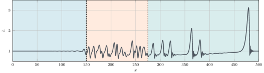
Figure 1: Example of developed flow for the Shkadov equations with $\delta=0.1$. Three regions can be identified: a first region where the instability grows from a white noise (blue), a second region with pseudo-periodic waves (orange), and a third region with non-periodic, pulse-like waves (green).

3.1.2 Discretization

Equations (1) are discretized using a finite difference approach. Due to the existence of sharp gradients, the convective terms are discretized using a TVD (total variation diminishing) scheme with a minmod flux limiter. The discretized third-order derivative is obtained by chaining a second-order centered difference for the second derivative with a second-order forward difference, leading to the following second-order approximation:

$$\begin{split}\left.\partial_{xxx}h\right|_{j}&\sim\frac{1}{2\Delta x^{3}}\left(-h_{j+3}+6h_{j+2}-12h_{j+1}+10h_{j}-3h_{j-1}\right)\\ &=\partial_{xxx}h(x_{j})+\frac{\Delta x^{2}}{4}\partial_{xxxxx}h(x_{j})+O\left(\Delta x^{3}\right).\end{split}$$ (4)

Finally, the time derivatives are discretized using a second-order Adams-Bashforth method:

$$h^{n+1}=h^{n}+\frac{\Delta t}{2}\left(-3f_{h}\left(h^{n}\right)+f_{h}\left(h^{n-1}\right)\right),$$ (5)

where $f_{h}$ represents the right hand side of the evolution equation of $h$ in system (1), and similarly for the $q$ field.

3.1.3 Environment

The proposed environment is re-implemented based on the original publication of Belus et al. [9], although with some significant differences. It is noted that the translational invariance feature introduced in [9] is not exploited here. Contrarily, this control problem is seen as an opportunity to test algorithms with a problem of arbitrarily high action dimensionality.

The control of the system (1) is performed by adding a forcing term $\delta q_{j}$ to the equation driving the temporal evolution of the flow rate. In practice, this is achieved by adding localized jets at certain positions in the domain, as shown below in figure 3, which intensities are to be controlled by the DRL agent. The first jet is positioned by default at $x_{0}=150$, with jet spacing being by default set to $\Delta x_{\text{jets}}=10$, similarly to [9]. To save computational time, the length of the domain is a function of the number of jets $n_{\text{jets}}$ and their spacing:

$$L=L_{0}+\left(n_{\text{jets}}+2\right)\Delta x_{\text{jets}}.$$ (6)

By default, $L_{0}=150$ (which corresponds to the start of the pseudo-periodic region for $\delta=0.1$), and $n_{\text{jets}}$ is set equal to 1. The spatial discretization step is set as $\Delta x=0.5$, while the numerical time step is $\Delta t=0.005$. The inlet noise level is set as $\varepsilon=$5\text{\times}{10}^{-4}$$, similarly to [9]. The injected flow rate $\delta q_{j}$ has the following form:

$$\delta q_{j}(x,t)=Au_{j}(t)\frac{4\left(x-x_{j}^{l}\right)\left(x_{j}^{r}-x\right)}{\left(x_{j}^{r}-x_{j}^{l}\right)^{2}},$$ (7)

with $A=5$ an ad-hoc non-dimensional amplitude factor, $x_{j}^{l}$ and $x_{j}^{r}$ the left and right limits of jet $j$, and $u_{j}(t)\in[-1,1]$ the action provided by the agent. Expression (7) corresponds to a parabolic profile of the jet in $x$, such that the injected flow rate drops to $0$ on the boundaries of each jet. The jet width $x_{j}^{r}-x_{j}^{l}$ is set equal to $4$, similarly to [9]. The time dependance of $u(t)$ is implemented as a saturated linear variation from one action to the next, in the form:

$$u_{j}(t)=(1-\alpha(t))u_{j}^{n-1}+\alpha(t)u_{j}^{n}\text{, with }\alpha(t)=\min\left(\frac{t-t_{n}}{\Delta t_{\text{int}}},1\right),$$ (8)

Hence, when the actor provides a new action to the environment at time $t=t_{n}$, the real imposed action is a linear interpolation between the previous action $u_{j}^{n-1}$ and the new action $u_{j}^{n}$ over a time $\Delta t_{\text{int}}$ (here taken equal to $0.01$ time units), after what the new action is imposed over the remaining action time $\Delta t_{\text{const}}$ (here taken equal to $0.04$ time units). The total action time-step is therefore $\Delta t_{\text{act}}=\Delta t_{\text{int}}+\Delta t_{\text{const}}$, which value is therefore equal to $0.05$ time units. The total episode time is fixed to $20$ time units, corresponding to $400$ actions.

The observations provided to the agent are the mass flow rates collected in the union of regions $A^{j}_{\text{obs}}$ of length $l_{\text{obs}}=10$ located upstream of each jet. Contrarily to the original article, the flow heights of this region are not provided to the agent, and the observations are not clipped.

The reward for each jet $j$ is computed on a region $A^{j}_{\text{rwd}}$ of length $l_{\text{rwd}}=10$ located downstream of it, the global reward consisting of a weighted sum of each individual reward:

$$r(t)=-\frac{1}{l_{\text{rwd}}\,n_{\text{jets}}}\sum_{j=0}^{n_{\text{jets}}-1}\sum_{x\in A^{j}_{\text{rwd}}}(h(x,t)-1)^{2}$$ (9)

Hence, the maximal reward is $0$ for a perfectly flat film, and the normalization factor allows to compare scores for problems of increasing complexity (i.e. with increasing number of jets).

Finally, each episode starts with the loading of a fully developed initial state obtained by solving the uncontrolled equations from an initial flat film configuration during a time $t_{\text{init}}=200$ time units. For convenience, this field is stored in a file and is loaded at the beginning of each episode. The initial state can be optionally made random by freely evolving the loaded initial configuration between $0$ and $20$ time units.

3.1.4 Results

The previously described environment is referred to as shkadov-v0, and its default parameters are provided in table 3. For the training, we set $n_{\text{rollout}}=3200$, $n_{\text{batch}}=2$, $n_{\text{epoch}}=32$ and $n_{\text{max}}=200k$. The related score curves are presented in 2(a). We also consider the training on the environment using $1$, $5$ and $10$ jets (see figure 2(b)). As could be expected, training is faster for small number of jets, while for larger amount of jets the ppo algorithm struggles due to the increasing dimensionality. In figure 3, we present the evolution of the field in time under the control of the agent for 5 jets using the default parameters. As can be observed, the agent quickly constrains the height of the fluid around $h=1$, before entering a quasi-stationary state in which a set of minimal jet actuations keeps the flow from developing instabilities in their direct vicinity. In the absence of jet further downstream, the instability regains in amplitude at the outlet of the domain. It must be noted that, due to the random upstream boundary condition, the environment is not deterministic, and therefore two exploitation runs with the same trained agent would lead to slightly different final scores.

Table 3: Default parameters for shkadov-v0!

L0	base length of domain	$150$
n_jets	number of jets	$5$
jet_pos	position of first jet	$150$
jet_space	spacing between jets	$10$
delta	physical parameter (2)	$0.1$

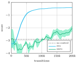
(a) Score curves with default parameters

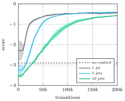
(b) Score curves for variable number of jets

Figure 2: Score curves for the shkadov-v0! environment in different configurations. (Left) Comparison of score curves for ppo and ddpg algorithms in the default configuration, using 5 jets. (Right) Comparison of different number of jets using the ppo algorithm. For each curve, we plot the average (solid color) and the standard deviation (shaded color) obtained from $n_{\text{training}}=5$ different runs. The dashed line indicates the reward obtained for the uncontrolled environment.

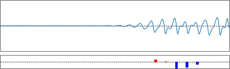
(a) $t=100$, start of control

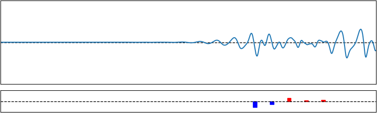
(b) $t=120$

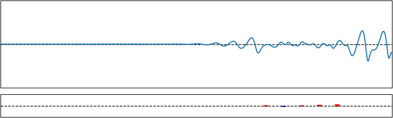
(c) $t=150$

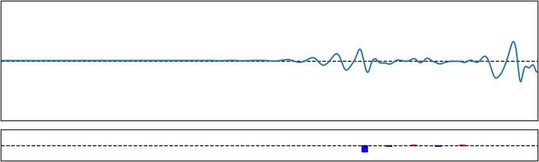
(d) $t=200$

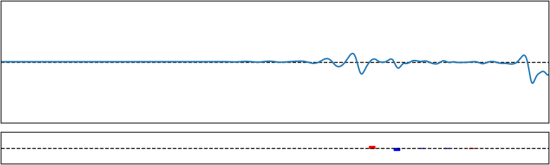
(e) $t=300$

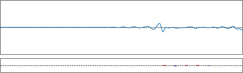
(f) $t=400$

Figure 3: Evolution of the flow under control of the agent, using 5 jets. The jets strengths are represented in the bottom rectangle (red means positive amplitude, blue means negative amplitude).

3.2 Rayleigh

3.2.1 Physics

We consider the resolution of the 2D Navier-Stokes equations coupled to the heat equation in a cavity of length $L$ and height $H$, with a hot bottom plate and cold top plate. Under favorable circumstances, this setup is known to lead to the Rayleigh-Bénard convection cell, illustrated in figure 4. The resulting system is driven by the following set of equations:

$$\begin{split}\nabla\cdot\bm{u}&=0,\\ \partial_{t}\bm{u}+(\bm{u}\cdot\nabla)\,\bm{u}&=-\nabla p+\sqrt{\frac{\text{Pr}}{\text{Ra}}}\nabla^{2}\bm{u}+\theta\bm{\hat{y}},\\ \partial_{t}\theta+(\bm{u}\cdot\nabla)\,\theta&=\frac{1}{\sqrt{\text{Pr}\,\text{Ra}}}\nabla^{2}\theta,\end{split}$$ (10)

where $\bm{u}$, $p$ and $\theta$ are respectively the non-dimensional velocity, pressure, and temperature of the fluid. The adimensional temperature $\theta$ is described in terms of the hot and cold reference temperatures, respectively denoted as $T_{H}$ and $T_{C}$:

$$\theta=\frac{T-\hat{T}}{\Delta T},\text{with }\hat{T}=\frac{T_{H}+T_{C}}{2}\text{ and }\Delta T=T_{H}-T_{C}.$$

The dynamics of the system (10) are controlled by two adimensional numbers. First, the Prandtl number Pr, which represents the ratio of the momentum diffusivity over the thermal diffusivity:

$$\text{Pr}=\frac{\nu}{\kappa},$$

where $\nu$ is the kinematic viscosity and $\kappa$ the thermal diffusivity. Second, the Rayleigh number Ra, which compares the characteristic time scales for transport due to diffusion and convection:

$$\text{Ra}=\frac{g\alpha\Delta TH^{3}}{\kappa\nu},$$

with $g$ the magnitude of the acceleration of the gravity and $\alpha$ the thermal expansion coefficient. We also define the instantaneous Nusselt number, Nu, as the adimensionalized heat flux averaged over the hot wall:

$$\text{Nu}(t)=-\int_{0}^{L}\partial_{y}\theta(x^{\prime},y=0,t)dx^{\prime}.$$ (11)

The system (10) is completed by the following initial and boundary conditions:

$$\begin{split}\bm{u}(x,y,0)=0&\text{ and }\theta(x,y,0)=0,\\ \bm{u}(x=0,y,t)=0&\text{ and }\bm{u}(x=L,y,t)=0,\\ \bm{u}(x,y=0,t)=0&\text{ and }\bm{u}(x,y=H,t)=0,\\ \theta(x,y=0,t)=\theta_{H}&\text{ and }\theta(x,y=H,t)=\theta_{C},\\ \partial_{x}\theta(x=0,y,t)=0&\text{ and }\partial_{x}\theta(x=L,y,t)=0,\end{split}$$ (12)

In essence, the boundary conditions (12) correspond to (i) a no-slip boundary conditions for the fluid on all boundaries, (ii) imposed hot and cold temperatures respectively on the bottom and top plate, and (iii) adiabatic boundary conditions on the lateral sides of the domain.

Above a critical value $\text{Ra}_{c}$, natural convection is triggered in the cell, increasing the heat exchange between the bottom and top regions of the cell, thus leading to $\text{Nu}>1$. Illustrations of the temperature and velocity fields are proposed in figure 4.

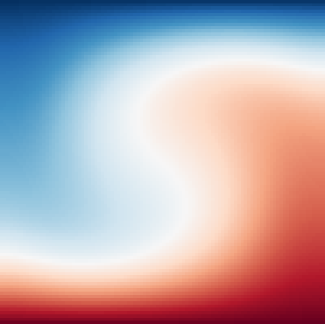
(a) Temperature

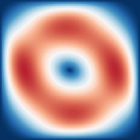
(b) Velocity norm

Figure 4: Temperature and velocity profiles for the uncontrolled Rayleigh convection cell with $\text{Ra}=$1\text{\times}{10}^{4}$$, $\text{Pr}=0.71$, $H=1$ and $L=1$.

3.2.2 Discretization

The system (10) is discretized using a structured finite volume incremental projection scheme with centered fluxes, in the fashion of [21]. For simplicity, the scheme is solved in a fully explicit way, except for the resolution of the Poisson equation for pressure. As is standard, a staggered grid is used for the finite volume scheme: the horizontal velocity is located on the west face of the cells, the vertical velocity is on the south face of the cells, while the pressure and temperature are located at the center of the cells. The computation of the instantaneous Nusselt number (11) is performed by computing the first-order finite difference of the temperature between the center of the first cell at the bottom of the mesh and the reference temperature $T_{H}$. Doing so, we obtain $\text{Nu}=2.16$ for $\text{Ra}=$1\text{\times}{10}^{4}$$ once the permanent regime is reached, which is close to the reference values found in the literature [22].

3.2.3 Environment

The proposed environment is re-implemented based on the original work of Beintema et al. [3]. In the following, we set $\text{Pr}=0.71$, which corresponds to the parameter for air, and $\text{Ra}=$1\text{\times}{10}^{4}$$ in order to avoid excessive computational loads. Similarly to [3], the control is performed by letting the DRL agent adjust the temperature of $n_{s}=10$ individual segments at the bottom of the cavity (see figure 5). To do so, the actions proposed by the agent are continuous temperature fluctuations $\left\{\hat{\theta}_{i}\right\}_{i\in\llbracket 0,n_{s}-1\rrbracket}$ in the range $\left[-C,+C\right]$, with $C=0.75$, $\theta_{H}=\frac{1}{2}$ and $\theta_{C}=-\frac{1}{2}$. To enforce $\left<\theta(y=0,x,t)\right>=\theta_{H}$ and $\theta(y=0,x,t)\in\left[\theta_{H}-C,\theta_{H}+C\right]$, the provided $\hat{\theta}_{i}$ are normalized as [3]:

$$\theta_{i}=\frac{\hat{\theta}_{i}-\left<\hat{\theta}\right>}{\max\left(1,\max_{j}\left(\frac{\hat{\theta}_{j}-\left<\hat{\theta}\right>}{C}\right)\right)}.$$ (13)

For simplicity, neither spatial nor temporal interpolations are performed between actions. The spatial discretization step is set as $\Delta x=0.02$, while the numerical time step is $\Delta t=0.01$. The action time-step $\Delta t_{\text{act}}$ is equal to $2$ time units, with the total episode length being fixed to $200$ time units, corresponding to $100$ actions.

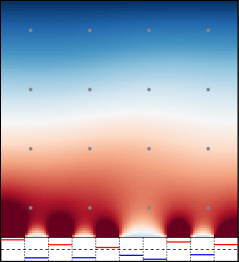
Figure 5: Observation probes and actions imposition for the rayleigh-v0! environment. The observations are collected at the probes regularly positioned in the domain, while the actions are imposed as piecewise-constant temperature boundary conditions on the bottom plate, with an average value equal to $\theta_{H}$.

The observations provided to the agent are the temperatures and the velocity components collected on a grid of $n_{p}\times n_{p}$ probes evenly spaced in the computational domain (see figure 5), plus the 3 previous observation vectors. The resulting set of observations is flattened in a vector of size $12\,n_{p}^{2}$, with a default value $n_{p}=4$.

The reward at each time-step is simply set as the negative instantaneous Nusselt number, such that increasing the reward corresponds to a decrease of the temperature convection:

$$r(t)=-\text{Nu}(t).$$ (14)

Finally, each episode starts with the loading of a fully developed initial state obtained by solving the uncontrolled equations during a time $t_{\text{init}}=200$ time units. The initial state corresponds to the field shown in figure 4. For convenience, this field is stored in a file and is loaded at the beginning of each episode.

3.2.4 Results

The environment as described in the previous section is referred to as rayleigh-v0, and its default parameters are provided in table 4. In this section, we note that the entropy bonus for the ppo agent is reduced to $\beta=0.001$ compared to the default hyperparameters of table 2. For the training, we set $n_{\text{rollout}}=1000$, $n_{\text{batch}}=2$, $n_{\text{epoch}}=32$ and $n_{\text{max}}=600k$. The score curves obtained are presented in 6, while the time evolution of the Nusselt for the controlled versus uncontrolled cases are shown in figure 7. As can be observed, the agent manages to devise a set of transition actions toward a stationary state with $\text{Nu}(t)=1$. The results of figure 7 are in line with those of [3]. In figure 8, we present the evolution of the temperature field during the first steps of the environment under the control of the agent using the default parameters.

Table 4: Default parameters used for rayleigh-v0!

L	length of the domain	$1$
H	height of the domain	$1$
n_sgts	number of control segments	$10$
ra	Rayleigh number	$1\text{\times}{10}^{4}$

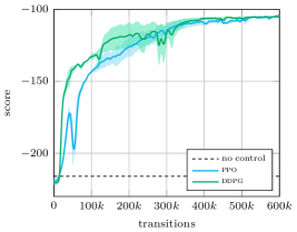
Figure 6: Score curves obtained using the ppo and the ddpg algorithms to solve the rayleigh-v0! environment. The dashed line indicates the reward obtained for the uncontrolled environment.

Figure 7: Evolution of the instantaneous Nusselt number during an episode of the rayleigh-v0! environment with and without control. The agent totally disables the convection, leading to a final Nusselt equal to $1$.

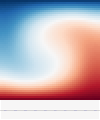
(a) $t=0$

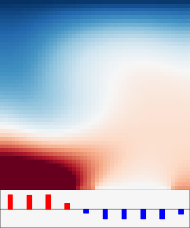
(b) $t=2$

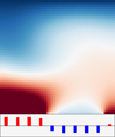
(c) $t=4$

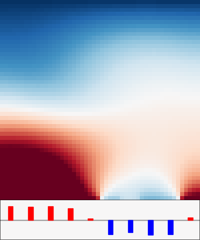
(d) $t=6$

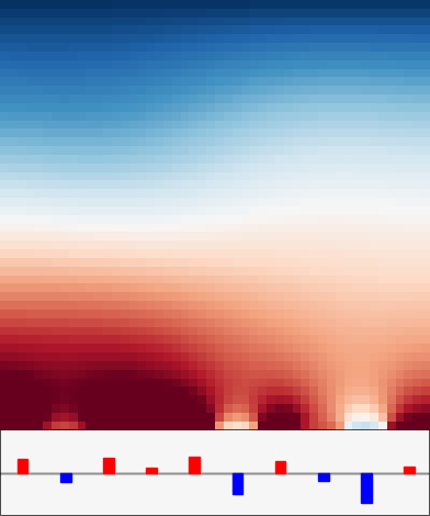
(e) $t=8$

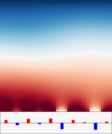
(f) $t=10$

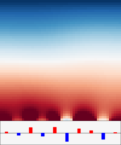
(g) $t=12$

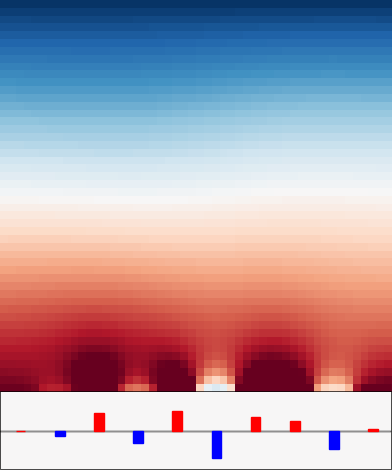
(h) $t=14$

Figure 8: Evolution of the convection cell under control of the agent, during the first steps of the environment. After a strong initial forcing, the agent establishes a pattern of alternating hot and cold actions that leads to a stationary configuration with $\text{Nu}(t)=1$. The control of the agent remains the same for the rest of the environment. The local temperature variations due to the control of the agent are represented in the bottom rectangle (red means positive amplitude, blue means negative amplitude).

3.3 Mixing

3.3.1 Physics

We consider the resolution of the 2D Navier-Stokes equations coupled to a passive scalar convection-diffusion equation in a cavity of length $L$ and height $H$ with moving boundary conditions on all sides. The resulting system is driven by the following set of equations:

$$\begin{split}\nabla\cdot\bm{u}&=0,\\ \partial_{t}\bm{u}+(\bm{u}\cdot\nabla)\,\bm{u}&=-\nabla p+\frac{1}{\text{Re}}\nabla^{2}\bm{u},\\ \partial_{t}c+(\bm{u}\cdot\nabla)\,c&=\frac{1}{\text{Pe}}\nabla^{2}c,\end{split}$$ (15)

where $\bm{u}$ and $p$ are respectively the non-dimensional velocity and pressure of the fluid, and $c$ is the concentration of a passive species. The dynamics of the system (15) are controlled by two adimensional numbers. First, the Reynolds number Re, which represents the ratio between inertial and viscous forces:

$$\text{Re}=\frac{UL}{\nu},$$

where $U$ and $L$ are respectively the reference velocity and length values, and $\nu$ is the kinematic viscosity of the fluid. Second, the Péclet number Pe, which represents the ratio between the advective and diffusive transport rates:

$$\text{Pe}=\frac{UL}{D},$$

where $D$ is the diffusion coefficient of the considered species. In essence, a system with a high Pe value presents a negligible diffusion, and scalar quantities move primarily due to fluid convection. The system (15) is completed by the following initial and boundary conditions:

$$\begin{split}\bm{u}(x,y,0)=0&\text{ and }c(x,y,0)=c_{0}\mathbb{1}_{\begin{subarray}{c}{x_{\text{min}}\leq x\leq x_{\text{max}}}\\ {y_{\text{min}}\leq y\leq y_{\text{max}}}\end{subarray}}\\ \bm{u}(x=0,y,t)=(0,v_{l})&\text{ and }\bm{u}(x=L,y,t)=(0,v_{r}),\\ \bm{u}(x,y=0,t)=(u_{b},0)&\text{ and }\bm{u}(x,y=H,t)=(u_{t},0),\\ \partial_{y}c(x,y=0,t)=0&\text{ and }\partial_{y}c(x,y=H,t)=0,\\ \partial_{x}c(x=0,y,t)=0&\text{ and }\partial_{x}c(x=L,y,t)=0,\end{split}$$ (16)

where $\mathbb{1}$ is the indicator function, and $v_{l}$, $v_{r}$, $u_{b}$ and $u_{t}$ are user-defined values. In essence, the boundary conditions (16) correspond to a multiple lid-driven cavity, where tangential velocity can be imposed independently on all sides, with an initial patch of concentration in the center of the domain. Snapshots of the evolution of the system in time with $(v_{l},v_{r},u_{b},u_{t})=(0,0,1.0,-1.0)$ are presented in figure 9.

(a) $t=0$

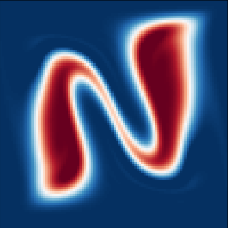
(b) $t=10$

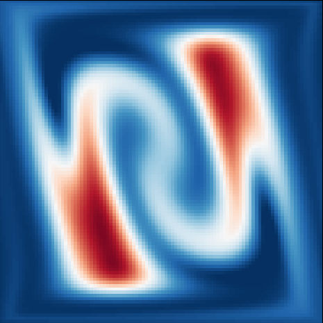
(c) $t=30$

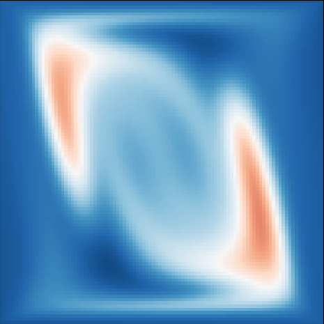
(d) $t=60$

Figure 9: Evolution of the concentration in time with constant boundary conditions $(v_{l},v_{r},u_{b},u_{t})=(0,0,1.0,-1.0)$.

3.3.2 Discretization

The system (15) is discretized using a structured finite volume incremental projection scheme with centered fluxes. For simplicity, the scheme is solved in a fully explicit way, except for the resolution of the Poisson equation for pressure. As is standard, a staggered grid is used for the finite volume scheme: the horizontal velocity is located on the west face of the cells, the vertical velocity is on the south face of the cells, while the pressure and concentration are located at the center of the cells.

3.3.3 Environment

In the following, we set $H=1$, $L=1$, $\Delta X=x_{\text{max}}-x_{\text{min}}=0.5$, $\Delta Y=y_{\text{max}}-y_{\text{min}}=0.5$, and $c_{0}=1$. The control is performed by letting the agent adjust the tangential velocities at the boundaries of the domain. We use a discrete action space of dimension $4$, with the following actions:

$$\begin{split}a=0&\iff(v_{l},v_{r},u_{b},u_{t})=(0,0,u_{\text{max}},-u_{\text{max}})\\ a=1&\iff(v_{l},v_{r},u_{b},u_{t})=(0,0,-u_{\text{max}},u_{\text{max}})\\ a=2&\iff(v_{l},v_{r},u_{b},u_{t})=(-u_{\text{max}},u_{\text{max}},0,0)\\ a=3&\iff(v_{l},v_{r},u_{b},u_{t})=(u_{\text{max}},-u_{\text{max}},0,0),\end{split}$$ (17)

where $u_{\text{max}}=\frac{\text{Re}\nu}{L}$. The non-dimensional numbers are chosen as $\text{Re}=100$ and $\text{Pe}=$1\text{\times}{10}^{4}$$, corresponding to a low diffusion species. For simplicity, no temporal interpolation is performed between actions. The spatial discretization step is set as $\Delta x=0.01$, while the numerical time step is $\Delta t=0.002$. The action time-step $\Delta t_{\text{act}}$ is equal to $0.5$ time units, with the total episode length being fixed to $50$ time units, corresponding to $100$ actions. The observations provided to the agent are the concentration and the velocity components collected on a grid of $n_{p}\times n_{p}$ probes evenly spaced in the computational domain, plus the 3 previous observation vectors. The resulting set of observations is flattened in a vector of size $12\,n_{p}^{2}$, with a default value $n_{p}=4$. The reward at each time-step is simply set as the average absolute distance of the concentration field to a target uniform value:

$$r(t)=-\lVert c-c_{t}\rVert_{1}\text{ with }c_{t}=\frac{\Delta X\Delta Y}{LH}c_{0}.$$ (18)

Finally, each episode starts with a null velocity field and an initial square patch of concentration $c_{0}$ as shown in figure 9(a).

3.3.4 Results

The environment as described in the previous section is referred to as mixing-v0, and its default parameters are provided in table 5. For the training, we set $n_{\text{rollout}}=2000$, $n_{\text{batch}}=2$, $n_{\text{epoch}}=32$ and $n_{\text{max}}=100k$. The score curves are presented in figure 10, along with the score obtained with constant control $a=0$, which leads to a score of approximately $-17.47$. For comparison, the score with no mixing at all (i.e.  pure diffusion) yields a score of $-28.78$. In figure 11, we present the evolution of the concentration field of the environment under the control of the agent using the default parameters.

Table 5: Default parameters used for mixing-v0!

L	length of the domain	$1$
H	height of the domain	$1$
re	Reynolds number	$1\text{\times}{10}^{2}$
pe	Péclet number	$1\text{\times}{10}^{4}$
side	initial side length of concentration patch	$0.5$
c0	initial concentration	$1$

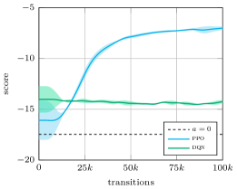
Figure 10: Score curves obtained using the ppo and the dqn algorithms to solve the mixing-v0! environment. The dashed line indicates the reward obtained for the uncontrolled environment.

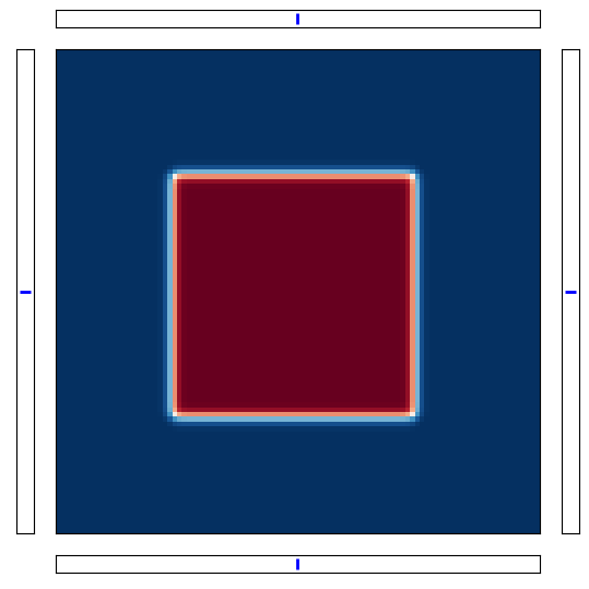
(a) $t=0$

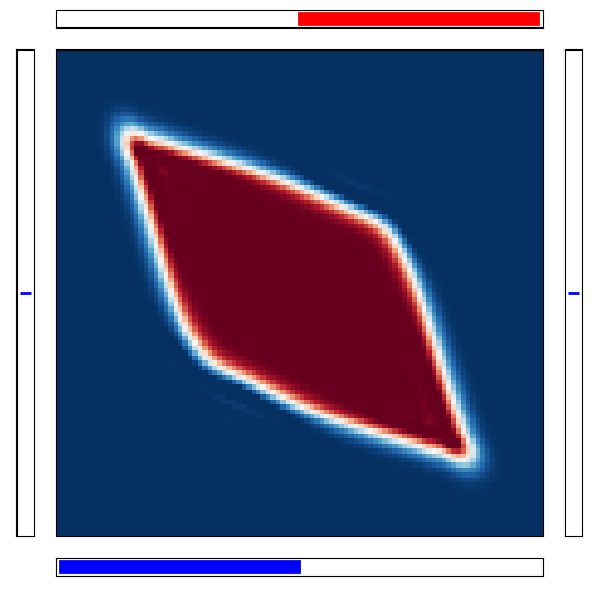
(b) $t=2$

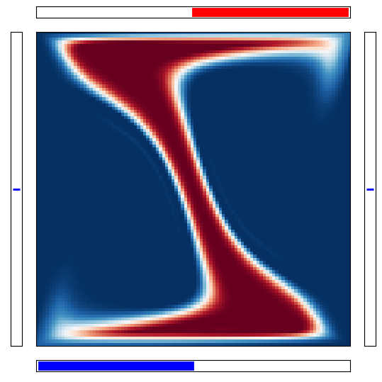
(c) $t=6$

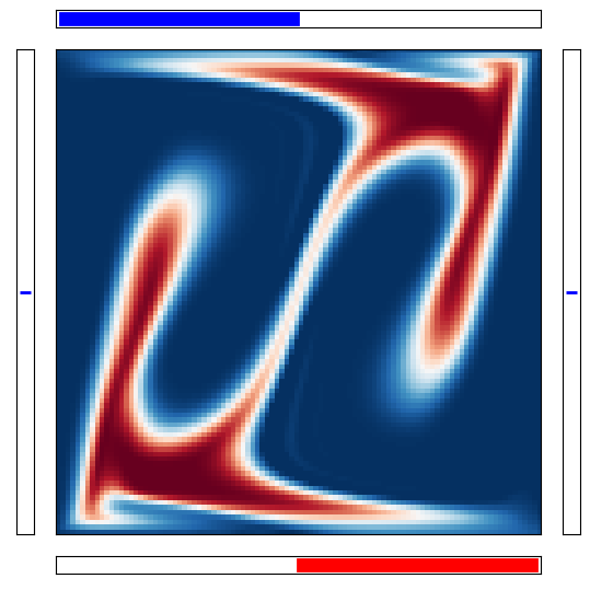
(d) $t=10$

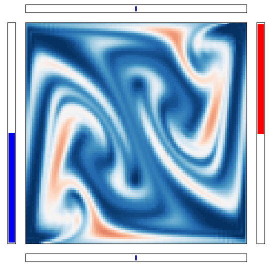
(e) $t=20$

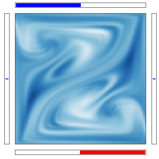
(f) $t=30$

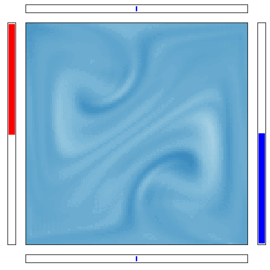
(g) $t=50$

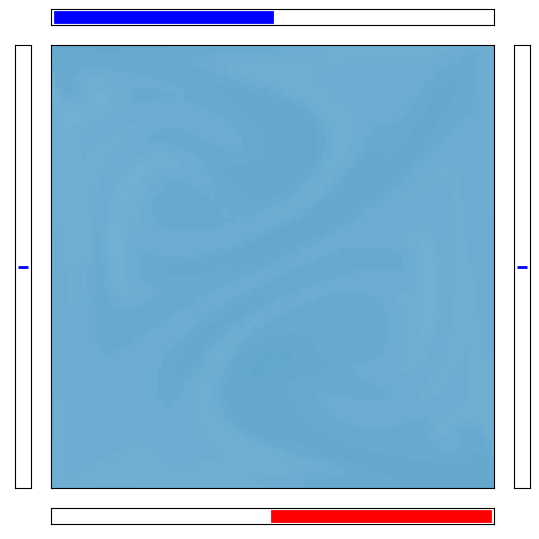
(h) $t=70$

Figure 11: Evolution of the mixing cell under control of the agent. The instantaneous controls are indicated with the four colored bars.

3.4 Lorenz

3.4.1 Physics

We consider the Lorenz attractor equations, a simple nonlinear dynamical system representative of thermal convection in a two-dimensional cell [23]. The set of governing ordinary differential equations reads:

$$\begin{split}\partial_{t}x&=\sigma(y-x),\\ \partial_{t}y&=x(\rho-z)-y,\\ \partial_{t}z&=xy-\beta z,\end{split}$$ (19)

where $\sigma$ is related to the Prandtl number, $\rho$ is a ratio of Rayleigh numbers, and $\beta$ is a geometric factor. Depending on the values of the triplet $(\sigma,\rho,\beta)$, the solutions to (20) may exhibit chaotic behavior, meaning that arbitrarily close initial conditions can lead to significantly different trajectories [24], one common such triplet being $(\sigma,\rho,\beta)=(10,28,8/3)$, that leads to the well-known butterfly shape presented in figure 12. The system has three possible equilibrium points, one in $(0,0,0)$ and one at the center of each ”wing” of the butterfly shape, which characteristics depend on the values of $\sigma$, $\rho$ and $\beta$.

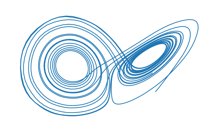
Figure 12: Control-free evolution of the Lorenz system. The attractor’s trajectory forms a distinctive, butterfly-like shape that consists of two large, symmetrically arranged lobes.

3.4.2 Discretization

The ODE system (20) is integrated in time with a five-stage, fourth-order low-storage Runge Kutta scheme from Carpenter et al. [25], using a constant time-step $\Delta t=0.05$. Similarly to [3], the numerical and action time-steps are taken equal.

3.4.3 Environment

The proposed environment is re-implemented based on the original work of Beintema et al. [3], where the goal is to maintain the system in the $x<0$ quadrant. The control (20) is performed by adding an external forcing term on the $\dot{y}$ equation:

$$\begin{split}\dot{x}&=\sigma(y-x),\\ \dot{y}&=x(\rho-z)-y+u,\\ \dot{z}&=xy-\beta z,\end{split}$$ (20)

with $u$ a discrete action in $\llbracket-1,0,1\rrbracket$. The action time-step is set to $\Delta t_{\text{act}}=0.05$ time units, and for simplicity no interpolation is performed between successive actions. A full episodes lasts $25$ time units, corresponding to $500$ actions. The observations are the variables $(x,y,z)$ and their time-derivatives $\dot{x},\dot{y},\dot{z}$, while the reward is set to $+1$ for each step with $x<0$, and $0$ otherwise. Each episode is started using the same initial condition $(x_{0},y_{0},z_{0})=(10,10,10)$.

3.4.4 Results

The environment as described in the previous section is referred to as lorenz-v0, and its default parameters are provided in table 6. For the training, we set $n_{\text{rollout}}=10000$, $n_{\text{batch}}=2$, $n_{\text{epoch}}=32$ and $n_{\text{max}}=2000k$. The related score curves are presented in figure 13. As can be observed, although the learning is successful, it is particularly noisy compared to some other environments presented in this library. This can be attributed to the chaotic behavior of the attractor, which makes the credit assignment difficult for the agent. A plot of the time evolutions of the controlled versus uncontrolled $x$ parameter is shown in figure 14. As can be observed, the agent successfully locks the system in the $x<0$ quadrant, with the typical control peak also observed by Beintema et al., noted with a red dot in figure 14. For a better visualization, several 3D snapshots of the controlled system are proposed in figure 15.

Table 6: Default parameters used for lorenz-v0!

sigma	Lorenz parameter	$10$
rho	Lorenz parameter	$28$
beta	Lorenz parameter	$\frac{8}{3}$

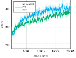
Figure 13: Score curves for the ppo and dqn algorithms when solving the lorenz-v0! environment. The dashed line indicates the reward obtained in the uncontrolled case.

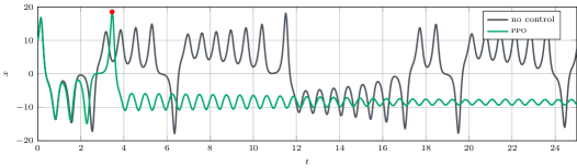
Figure 14: Controlled versus uncontrolled time evolution of the $x$ parameter. The red dot corresponds to the typical control peak that precedes the locking of the system, also observed in [3].

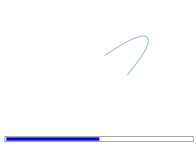
(a) $t=5$

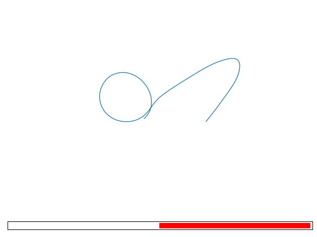
(b) $t=25$

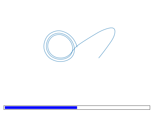
(c) $t=50$

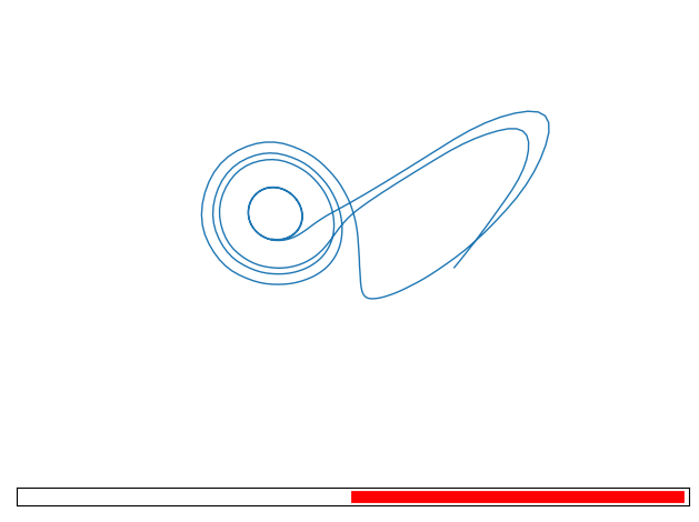
(d) $t=100$

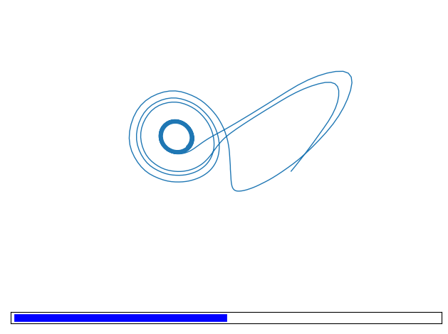
(e) $t=200$

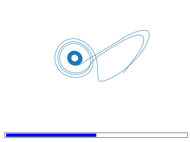
(f) $t=300$

Figure 15: Evolution of the controlled Lorenz system using the ppo algorithm. The instantaneous control value is indicated at the bottom by the colored bar (blue is for $-1$, red is for $+1$).

3.5 Burgers

3.5.1 Physics

The inviscid Burgers equation was first introduced by Bateman in 1915, and models the behavior of a one-dimensional inviscid incompressible fluid flow [26], before being studied by Burgers in 1948 [27]:

$$\partial_{t}u+u\partial_{x}u=0.$$ (21)

We consider the resolution of the Burgers equation on a domain of length $L$, along with the following initial and boundary conditions:

$$\begin{split}u(x,0)&=u_{\text{target}},\\ u(0,t)&=u_{\text{target}}+\mathcal{U}(-\sigma,\sigma),\\ \partial_{x}u(L,t)&=0,\end{split}$$ (22)

where $\sigma$ is the noise level introduced at the inlet, and $u_{\text{target}}$ is a constant value. The convection of the random inlet signal leads to a noisy solution in the domain, as is depicted in figure 16. The initial perturbations steepen while propagating downstream to eventually form shocks.

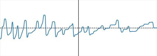
Figure 16: Uncontrolled solution of the Burgers equation with uniform random noise excitation at the inlet. The vertical bar indicates the position of the controller.

3.5.2 Discretization

The Burgers equation (21) is discretized in time with a finite volume approach. The convective term is discretized using a TVD scheme with a Van Leer flux limiter, while the time marching is performed using a second-order finite-difference scheme.

3.5.3 Environment

The goal of the environment is to control a pointwise forcing source term $a(t)$ on the right-hand side of (21), in order to damp the noise transported from the inlet. The forcing is applied at $x_{p}=1$, while the length of the domain is set to $L=2$. The actions provided to the environment, which are expected to be in $\left[-1,1\right]$, are then scaled by an ad-hoc non-dimensional amplitude factor $A=10$. The field is initially set equal to $u_{\text{target}}=0.5$, and the variance of the inlet noise is chosen to be $\sigma=0.1$. The spatial discretization step is set to $\Delta x=$4\text{\times}{10}^{-3}$$, while the numerical time-step is equal to $\Delta t=$8\text{\times}{10}^{-4}$$ time units. The action duration is set to $\Delta t_{\text{act}}=0.05$ time units, for a total episode duration equal to $10$ time units, corresponding to $200$ actions. The observations provided to the agent are the $n_{\text{obs}}=5$ values of $u$ upstream of the actuator. Finally, the reward is computed as:

$$r(t)=-\Delta x\norm{u(x,t)-u_{\text{target}}}_{1}\text{ with }x\in\left[x_{p},L\right].$$ (23)

3.5.4 Results

The environment as described in the previous section is referred to as burgers-v0, and its default parameters are provided in table 7. For the training, we set $n_{\text{rollout}}=4000$, $n_{\text{batch}}=2$, $n_{\text{epoch}}=32$ and $n_{\text{max}}=500k$. The score curves obtained are shown in figure 17, while snapshots of the evolution of the controlled environment are shown in figure 18. As can be observed, the agent successfully damps the transported inlet noise following an opposition control strategy.

Table 7: Default parameters used for burgers-v0!

L	domain length	$2$
u_target	target value	$0.5$
sigma	inlet noise level	$0.1$
amp	control amplitude	$10$
ctrl_pos	control position	$1$

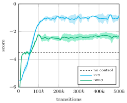
Figure 17: Score curves for the ppo and the ddpg algorithms when solving the burgers-v0! environment. The dashed line indicates the reward obtained for the uncontrolled case.

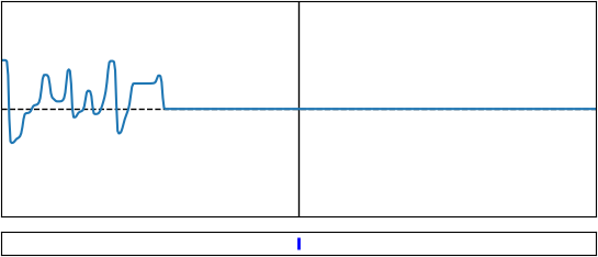
(a) $t=20$

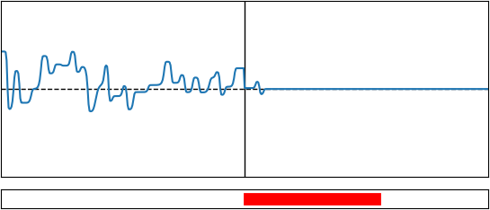
(b) $t=40$

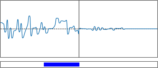
(c) $t=60$

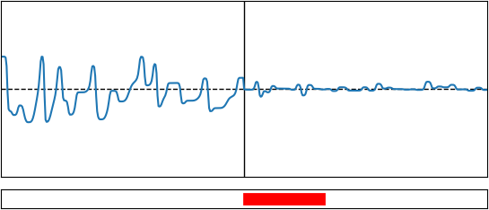
(d) $t=100$

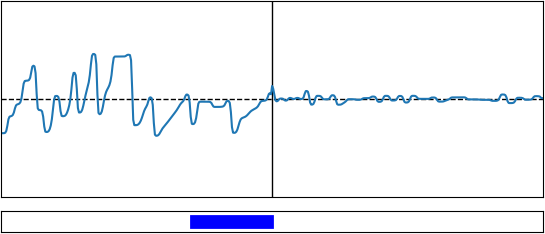
(e) $t=150$

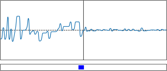
(f) $t=200$

Figure 18: Evolution of the controlled burgers system using the ppo algorithm. The instantaneous control value is indicated at the bottom by the colored bar (blue is for negative actuations, while red is for positive ones).

3.6 Sloshing

3.6.1 Physics

We consider the resolution of the 1D Saint-Venant equations (or shallow water equations), established in 1871 [28], which describe a shallow layer of fluid in hydrostatic balance with constant density. This system is considered in the context of a mobile water tank of length $L$ subjected to an acceleration $\ddot{y}$, leading to the following equations in the tank referential [29]:

$$\begin{split}\partial_{t}h&=-\partial_{x}q,\\ \partial_{t}q&=-\partial_{x}\left(\frac{q^{2}}{h}+\frac{1}{2}gh^{2}\right)-\ddot{y},\end{split}$$ (24)

where $h$ is the fluid height, and $q$ is the fluid flow rate. The system (24) is completed by the following initial and boundary conditions:

$$\begin{split}q(x,0)=0&\text{ and }h(x,0)=1,\\ q(0,t)=0&\text{ and }\partial_{x}h(0,t)=0,\\ q(L,t)=0&\text{ and }\partial_{x}h(L,t)=0.\end{split}$$ (25)

The situation is summed up in figure 19. When laterally excited, the surface of the fluid sloshes back and forth in the tank generating complex patterns at the fluid surface, as shown in figure 20. When the excitation stops, a relaxation phase is observed, usually leaving a single wavefront travelling back and forth in the tank until it dissipates entirely. Due to its simplicity, the model (24) does not allow wave breaking nor the formation of drops on the sides of the domain.

Figure 19: Configuration of the sloshing tank. The fluid flow is determined by the fluid height $h(x,t)$ and by its mass flow rate $q(x,t)$. The movement of the tank is controlled by its acceleration $\ddot{y}(t)$.

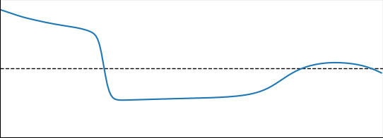
(a) Excitation phase

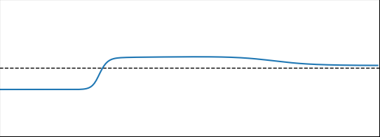
(b) Relaxation phase

Figure 20: Examples of fluid surface during the excitation phase (left) and the relaxation phase (right). The fluid height at rest is $h=1$, indicated by the dotted line.

3.7 Discretization

The system (24) is discretized using a finite volume scheme with Rusanov fluxes [30], which is an improved form of the Lax-Friedrichs flux. The time derivatives for both $h$ and $q$ are discretized using the second-order Adams-Bashforth scheme.

3.8 Environment

The control of the system (24) is performed through the cart acceleration term $\ddot{y}$. The system is first set in motion during $t_{\text{exc}}=2$ time units using a sinusoid-based signal:

$$\ddot{y}_{\text{exc}}(t)=\frac{1}{2}\left(\cos(\pi t)+3\cos(4\pi t)\right).$$ (26)

The resulting fields are stored in a file for simplicity, and loaded at the beginning of each episode. By default, the length of the cart is $L=2.5$, the spatial discretization corresponds to $100$ finite volume cells per unit of length, and the numerical time step is $\Delta t=0.001$ time units. The actions provided to the environment, which are expected to be in $\left[-1,1\right]$, are then scaled by an ad-hoc non-dimensional amplitude factor $A=5$. The interpolation between successive actions is identical to (8), with $\Delta t_{\text{int}}=0.01$ time units and $\Delta t_{\text{act}}=0.05$ time units. The total episode time is fixed to $10$ time units, corresponding to $200$ actions. The observations provided to the agent are the heights collected on the entire domain. To limit the size of the resulting vector, it is downsampled by a factor 2. Finally, the reward signal is defined as:

$$r(t)=-\Delta x\norm{h(x,t)-1}_{2}-\alpha\left|\ddot{y}(t)\right|,$$ (27)

where $\norm{\cdot}_{2}$ is the $2$-norm and $\alpha=0.0005$. The $\Delta x$ factor allows to obtain comparable reward values for variable discretization levels.

3.9 Results

The environment as described in the previous section is referred to as sloshing-v0, and its default parameters are provided in table 8. For the training, we set $n_{\text{rollout}}=2000$, $n_{\text{batch}}=2$, $n_{\text{epoch}}=16$ and $n_{\text{max}}=200k$. The score curves are presented in figure 21, while the time evolutions of the controlled versus uncontrolled fluid level are shown in figure 22. As can be observed, the agent manages to roughly cut the uncontrolled reward in half, by suppressing the back and forth wavefront using large actuations in the early stages of control, after what the control amplitude drops significantly.

Table 8: Default parameters used for sloshing-v0!

L	length of the tank	$2.5$
amp	amplitude of the control	$5$
alpha	control penalization	$0.0005$
g	gravity acceleration	$9.81$

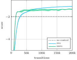
Figure 21: Score curves for the sloshing-v0! environment using the ppo and the ddpg algorithms. The dashed line indicates the reward obtained for the uncontrolled environment.

     

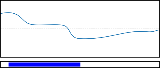
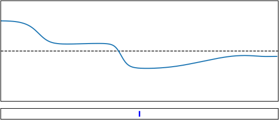
(a) $t=0$

     

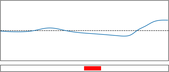
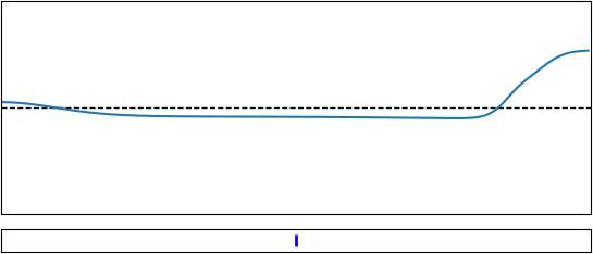
(b) $t=0.5$

     

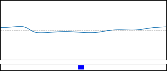
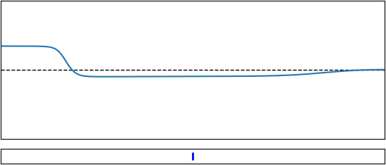
(c) $t=1.5$

     

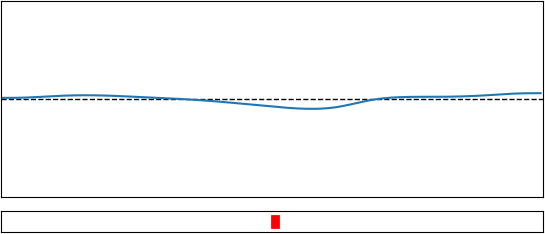
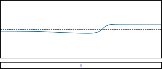
(d) $t=2.5$

     

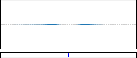
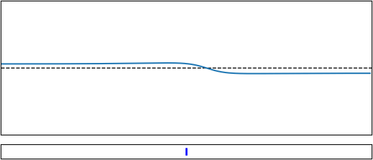
(e) $t=5$

     

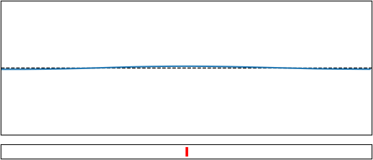
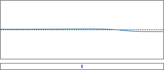
(f) $t=10$

Figure 22: Evolution of the fluid surface with (left) and without (right) agent control. The control amplitude and direction is represented using the rectangle at the bottom (red means positive, blue means negative).

3.10 Vortex

3.10.1 Physics

We consider the resolution of a dynamical system modeling the nonlinear vortex-induced vibrations of a rigid circular cylinder. The flow motion is governed by the incompressible Navier–Stokes equations, whereas the cylinder motion is a simple translation governed by a linear mass-damper-spring equation affected by the fluid loading. This is modeled by coupled amplitude equations derived in [31, 32] after dominant balance arguments:

$$\begin{split}\partial_{t}A&=\lambda\left(\frac{1}{\text{Re}_{*}}-\frac{1}{\text{Re}}\right)A-\mu A\lvert A\rvert^{2}+\alpha Y\\ \partial_{t}Y&=\left(-\omega_{*}\gamma+\mathrm{i}\left(\omega_{s}-\omega_{*}\right)\right)Y+\frac{\beta}{\omega_{*}m}A\end{split}$$ (28)

where $A$ and $Y$ are unknown slow time-varying, complex amplitudes modeling respectively the flow disturbances and the cylinder center of mass, $\text{Re}=50$ is the Reynolds number, $\text{Re}_{*}=46.6$ is the threshold of instability of the steady cylinder, $\omega_{*}=0.74$ is the frequency of the marginally stable eigenmode classically computed from the flow past a fixed cylinder [33], $\omega=1.1$ is the dimensionless natural frequency of the cylinder in vacuum, $\gamma=0.023$ is the structural damping coefficient, and $m=10$ is the ratio of the solid to the fluid densities. The coefficients $\lambda$, $\mu$, $\alpha$, $\beta$ in (30) are analytically computable from an asymptotic analysis of the coupled flow-cylinder system, their numerical value being taken from [31] as:

$$\lambda=9.153+3.239\mathrm{i},\quad\mu=308.9-1025\mathrm{i},\quad\alpha=0.03492+0.01472\mathrm{i},\quad\beta=1.$$ (29)

The ability of the model to reproduce the physics of vortex-induced vibrations has been assessed from the study of the nonlinear limit cycles, i.e. the periodic, synchronized orbits reached by the system at large time whose analytical expressions are reported in [31]. Of particular importance is the simultaneous existence of multiple stable cycles (either a single limit cycle, or three over specific ranges of frequencies), that is shown to trigger a complex hysteretic behavior in the lock-in regime. Since all limit cycle solutions are periodic, the mean mechanical energy averaged over a period is zero, and the mean work received from the fluctuating lift force is entirely dissipated by structural damping. As discussed in [31], it follows that the leading order mean dissipated energy is a simple quadratic function of the displacement amplitude, meaning that only the upper limit cycle (the one limit cycle yielding the largest displacement amplitude) is of practical interest for the energy extraction problem, that is, in cases where one seeks to leverage such vortex-induced vibrations to generate electrical energy, for instance by having the oscillation of the cylinder displace periodically a magnet within a coil.

In essence, it can be inferred that there must exist an optimal structural parameter setting for which the dissipated energy is maximum: on the one hand, the flow-cylinder system must be synchronized for the cylinder displacement amplitude to be large. On the other hand, the energy tends to zero in the limit $\gamma\gg 1$ where the work received from the lift force is limited by the low amplitude of the displacement, and in the limit $\gamma\ll 1$ where the displacement is self-limited. As evidenced in [32], the problem shown is that the optimum lies at the edge of a discontinuity, corresponding to parameter settings where the system undergoes a transition from a hysteretic to a non-hysteretic regime. This has important consequences for the application, since small inaccuracies in the structural parameters of small external flow disturbances may tip the system outside the hysteresis zone and lead to convergence to cycles of lower energy, resulting in a dramatic drop of the harnessed energy.

3.11 Discretization

The system (30) is integrated in time using a five-stage, fourth-order low-storage Runge Kutta scheme from Carpenter et al. [25], using a constant time-step $\Delta t=0.1$.

3.12 Environment

The proposed environment is re-implemented based on the original work of [32], where the goal is to maximize the cylinder displacement and bypass the existence of low energy cycles. This is achieved adding a proportional feedback control in the structure equation, assuming that the state of the system is accessed through measurements of the flow disturbances position, and that an actuator applies at the surface of the cylinder a control velocity:

$$\begin{split}\partial_{t}A&=\lambda\left(\frac{1}{\text{Re}_{*}}-\frac{1}{\text{Re}}\right)A-\mu A\lvert A\rvert^{2}+\alpha Y+ke^{\mathrm{i}\phi}A\\ \partial_{t}Y&=\left(-\omega_{*}\gamma+\mathrm{i}\left(\omega_{s}-\omega_{*}\right)\right)Y+\frac{\beta}{\omega_{*}m}A\end{split}$$ (30)

with $k$ the gain and $\phi$ the phase shift between the measure and the action. The actions provided to the environment, which are expected to be in $\left[-1,1\right]$, are rescaled to $\left[0,0.3\right]$ for the module, and $\left[-\pi,\pi\right]$ for the phase. The action time-step is set to $\Delta t_{\text{act}}=0.5$ time units, a full episode lasting $400$ time units, corresponding to $800$ actions. The observations are the complex variables $A$ and $Y$ as well as their time-derivatives, leading to an observation vector of size $8$. The reward at each time-step is computed as:

$$r(t)=8\omega_{s}\gamma\left(\frac{\text{d}}{\text{d}t}\left[Ye^{\mathrm{i}\omega_{*}t}\right]\right)^{2}-2w\left[ke^{\mathrm{i}\phi}Ae^{\mathrm{i}\omega_{*}t}\right]^{2},$$ (31)

where the leftmost term is the mean dissipated energy and is thus associated to performance, the rightmost term estimates the mean kinetic energy expended by the actuator over a limit cycle period and is thus associated to cost, and $w$ is a weighting coefficient set empirically to $50$ (a value found to be large enough for cost considerations to impact the optimization procedure, but not so large as to dominate the reward signal, in which case actuating is meaningless). Each episode begins using the same initial condition $(A_{0},Y_{0})=\left(-0.00385-0.00378\mathrm{i},0.00118-0.00131\mathrm{i}\right)$ that, in the absence of control, leads convergence to a low limit cycle, for which the score is equal to $0.00607$.

3.13 Results

The environment as described in the previous section is referred to as vortex-v0, and its default parameters are provided in table 9. For the training, we set $n_{\text{rollout}}=4000$, $n_{\text{batch}}=2$, $n_{\text{epoch}}=32$ and $n_{\text{max}}=1000k$. The score curves are presented in figure 23, while the time evolutions of the controlled versus uncontrolled fluid level are shown in figure 24. As can be observed, the agent manages to lock in a high limit cycle, with a final score more than 3 orders of magnitude larger than that of the uncontrolled low limit cycle, and twice as large as that of the uncontrolled high limit cycle (whose score computed using $A_{0}=Y_{0}=0.05(1+\mathrm{i})$ is $19.25$).

Table 9: Default parameters used for vortex-v0!

re	Reynolds number	$50$
w	control penalization	$50$

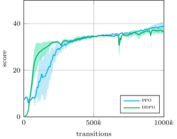
Figure 23: Score curves for the vortex-v0! environment using the ppo and the ddpg algorithms. The uncontrolled environment obtains a score of $0.00607$ when locking in on the low limit cycle.

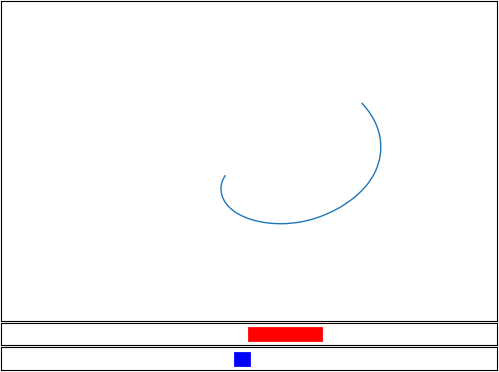
(a) $t=25$

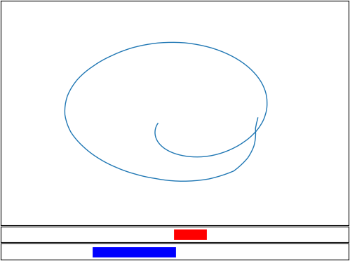
(b) $t=50$

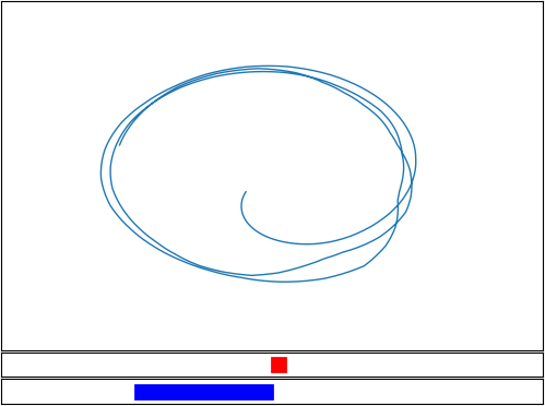
(c) $t=100$

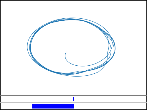
(d) $t=200$

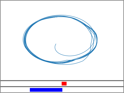
(e) $t=300$

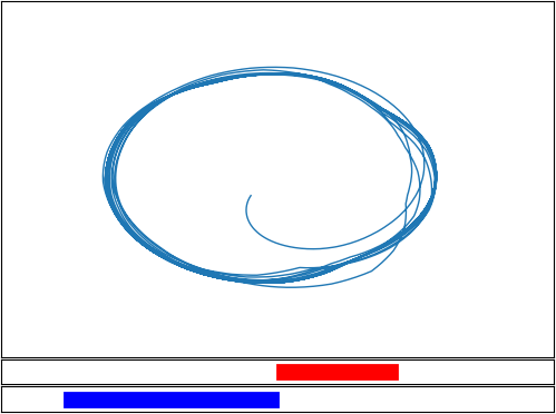
(f) $t=800$

Figure 24: Evolution of the controlled vortex system using the ddpg algorithm. The instantaneous control values are indicated at the bottom by the colored bars.

4 Availability and conclusion

The sources of the present work are made open-source on the following repository: https://github.com/jviquerat/beacon. While the present version of the library presents a variety of phenomena and control types, its purpose is to grow with new cases proposed by the community, within the constraints defined in section 2. To this end, issues and pull requests are accepted on the library repository.

Funding

Funded/co-funded by the European Union (ERC, CURE, 101045042). Views and opinions expressed are however those of the author(s) only and do not necessarily reflect those of the European Union or the European Research Council. Neither the European Union nor the granting authority can be held responsible for them.

References

- [1] Y.-Z. Wang, Y.-F. Mei, and N. Aubry. Deep reinforcement learning based synthetic jet control on disturbed flow over airfoil. Physics of Fluids, 34:033606, 2022.
- [2] G. Novati, S. Verma, D. Alexeev, D. Rossinelli, W. M. van Rees, and P. Koumoutsakos. Synchronisation through learning for two self-propelled swimmers. Bioinspiration & Biomimetics, 12(3):036001, 2017.
- [3] G. Beintema, A. Corbetta, L. Biferale, and F. Toschi. Controlling rayleigh–bénard convection via reinforcement learning. Journal of Turbulence, 21(9-10):585–605, 2020.
- [4] M. Andrychowicz, A. Raichuk, P. Stańczyk, M. Orsini, S. Girgin, R. Marinier, L. Hussenot, M. Geist, O. Pietquin, M. Michalski, S. Gelly, and O. Bachem. What matters in on-policy reinforcement learning? a large-scale empirical study. arXiv preprint arXiv:2006.05990, 2020.
- [5] E. Todorov, T. Erez, and Y. Tassa. Mujoco: A physics engine for model-based control. In 2012 IEEE/RSJ International Conference on Intelligent Robots and Systems, pages 5026–5033. IEEE, 2012.
- [6] M. G. Bellemare, Y. Naddaf, J. Veness, and M. Bowling. The arcade learning environment: An evaluation platform for general agents. Journal of Artificial Intelligence Research, 47:253–279, 2013.
- [7] J. Rabault and A. Kuhnle. Accelerating deep reinforcement learning strategies of flow control through a multi-environment approach. Physics of Fluids, 31(9):094105, 2019.
- [8] J. Viquerat and E. Hachem. Parallel bootstrap-based on-policy deep reinforcement learning for continuous fluid flow control applications. Fluids, 8(7), 2023.
- [9] V. Belus, J. Rabault, J. Viquerat, Z. Che, E. Hachem, and U. Reglade. Exploiting locality and translational invariance to design effective deep reinforcement learning control of the 1-dimensional unstable falling liquid film. AIP Advances, 9(12):125014, 2019.
- [10] S. K. Lam, A. Pitrou, and S. Seibert. Numba: A llvm-based python jit compiler. In Proceedings of the Second Workshop on the LLVM Compiler Infrastructure in HPC, 2015.
- [11] G. Brockman, V. Cheung, L. Pettersson, J. Schneider, J. Schulman, J. Tang, and W. Zaremba. Openai gym. arXiv preprint arXiv:1606.01540, 2016.
- [12] C. R. Harris, K. J. Millman, S. J. van der Walt, R. Gommers, P. Virtanen, D. Cournapeau, E. Wieser, J. Taylor, S. Berg, N. J. Smith, R. Kern, M. Picus, S. Hoyer, M. H. van Kerkwijk, M. Brett, A. Haldane, J. Fernández del Río, M. Wiebe, P. Peterson, P. Gérard-Marchant, K. Sheppard, T. Reddy, W. Weckesser, H. Abbasi, C. Gohlke, and T. E. Oliphant. Array programming with NumPy. Nature, 585(7825):357–362, 2020.
- [13] J. D. Hunter. Matplotlib: A 2d graphics environment. Computing in Science & Engineering, 9(3):90–95, 2007.
- [14] J. Schulman, F. Wolski, P. Dhariwal, A. Radford, and O. Klimov. Proximal policy optimization algorithms. arXiv preprint arXiv:1707.06347, 2017.
- [15] P. L. Kapitza. Wave flow of a thin viscous fluid layers. Zhurnal Eksperimental’noi i Teoreticheskoi Fiziki, 18:3–18, 1948.
- [16] V. Y. Shkadov. Wave flow regimes of a thin layer of viscous fluid subject to gravity. Fluid Dynamics, 2:29–34, 1967.
- [17] G. Lavalle. Integral modeling of liquid films sheared by a gas flow. PhD thesis, ISAE - Institut Supérieur de l’Aéronautique et de l’Espace, 2014.
- [18] H. C. Chang, E. A. Demekhin, and S. S. Saprikin. Noise-driven wave transitions on a vertically falling film. Journal of Fluid Mechanics, 462:255–283, 2002.
- [19] H. C. Chang and E. A. Demekhin. Complex wave dynamics on thin films. Elsevier, 2002.
- [20] A. Koulago and D. Parséghian. A propos d’une équation de la dynamique ondulatoire dans les films liquides. Journal de Physique III, 5(3):309–312, 1995.
- [21] S. Boivin, F. Cayré, and J.-M. Hérard. A finite volume method to solve the navier–stokes equations for incompressible flows on unstructured meshes. International Journal of Thermal Sciences, 39(8):806–825, 2000.
- [22] N. Ouertatani, N. Ben Cheikh, B. Ben Beya, and T. Lili. Numerical simulation of two-dimensional rayleigh–bénard convection in an enclosure. Comptes Rendus Mécanique, 336(5):464–470, 2008.
- [23] B. Saltzman. Finite amplitude free convection as an initial value problem. Journal of atmospheric sciences, 19(4):329–341, 1962.
- [24] E. N. Lorenz. Deterministic nonperiodic flow. Journal of Atmospheric Sciences, 20(2):130–141, 1963.
- [25] M. H. Carpenter and C. A. Kennedy. Fourth-order 2n-storage Runge-Kutta schemes. Technical report, National Aeronautics and Space Administration, 1994.
- [26] H. Bateman. Some recent researches on the motion of fluids. Monthly Weather Review, 43(4):163–170, 1915.
- [27] J. M. Burgers. A mathematical model illustrating the theory of turbulence. Advances in Applied Mechanics, 1:171–199, 1948.
- [28] A.J.C Saint-Venant. Théorie du mouvement non permanent des eaux, avec application aux crues des rivières et a l’introduction de marées dans leurs lits. Comptes Rendus des Séances de Académie des Sciences, 73, 1871.
- [29] T. Berger, M. Puche, and F. L. Schwenninger. Funnel control for a moving water tank. Automatica, 135:109999, 2022.
- [30] S. Cordier, F. Darboux, O. Delestre, and F. James. étude d’un modèle de ruissellement 1d. Technical report, Univ. Orléans, INRA, 2007.
- [31] P. Meliga and J.-M. Chomaz. An asymptotic expansion for the vortex-induced vibrations of a circular cylinder. Journal of Fluid Mechanics, 671:137–167, 2011.
- [32] P. Meliga, J.-M. Chomaz, and F. Gallaire. Extracting energy from a flow: An asymptotic approach using vortex-induced vibrations and feedback control. Journal of Fluids and Structures, 27:861–874, 2011.
- [33] D. Barkley. Linear analysis of the cylinder wake mean flow. Europhysics Letters, 75:750, 2006.