Ultraviolet and Chromospheric activity and Habitability of M stars

Abstract

M-type stars are crucial for stellar activity studies since they cover two types of magnetic dynamos and particularly intriguing for habitability studies due to their abundance and long lifespans during the main-sequence stage. In this paper, we used the LAMOST DR9 catalog and the GALEX UV archive data to investigate the chromospheric and UV activities of M-type stars. All the chromospheric and UV activity indices clearly show the saturated and unsaturated regimes and the well-known activity-rotation relation, consistent with previous studies. Both the FUV and NUV activity indices exhibit a single-peaked distribution, while the H$\alpha$ and Ca II H$\&$K indices show a distinct double-peaked distribution. The gap between these peaks suggests a rapid transition from a saturated population to an unsaturated one. The smoothly varying distributions of different subtypes suggest a rotation-dependent dynamo for both early-type (partly convective) to late-type (fully convective) M stars. We identified a group of stars with high UV activity above the saturation regime (log$R^{\prime}_{\rm NUV}>-2.5$) but low chromospheric activity, and the underlying reason is unknown. By calculating the continuously habitable zone and the UV habitable zone for each star, we found about 70% stars in the total sample and 40% stars within 100 pc are located in the overlapping region of these two habitable zones, indicating a number of M stars are potentially habitable. Finally, we examined the possibility of UV activity studies of M stars using the China Space Station Telescope.

1 INTRODUCTION

M-type stars are thought to exhibit stronger magnetic activity compared to other types of stars. Numerous studies have been conducted to investigate the stellar activities of M-type stars, by using X-ray (e.g., Stelzer et al., 2013; Wright & Drake, 2016), H$\alpha$ emission (e.g., Douglas et al., 2014; Newton et al., 2017), Ca II H$\&$K emission (e.g., Astudillo-Defru et al., 2017; Boro Saikia et al., 2018; Lehtinen et al., 2020), UV emission (e.g., Stelzer et al., 2013; Schneider & Shkolnik, 2018; Richey-Yowell et al., 2023), and optical flare (e.g., Yang et al., 2017), etc. These investigations aim to understand the manifestations of stellar activity and its connection to the stellar dynamo. For early M stars, they typically follow the solar-type dynamo mechanism ($\alpha$-$\Omega$ dynamo or tachocline dynamo). The generation of magnetic fields occurs in their deep convection zones due to the interior radial differential rotation, and the magnetic fields are then amplified through the interaction between magnetic flux tubes and convection processes (e.g., Parker, 1975; Reid & Hawley, 2000). On the other hand, late M stars, which are fully convective, lack a tachocline and exhibit a different dynamo mechanism, such as the $\alpha^{2}$ dynamo. Therefore, M-type stars offer a unique opportunity to study two different magnetic dynamos within a single stellar type.

Since M-type stars constitute approximately 70% of the total stellar population in the Milky Way (Bochanski et al., 2009), there is significant interest in investigating the habitable zones and potentially habitable planets around M stars. Thanks to recent space missions like Kepler and TESS, several habitable planets have been identified orbiting M stars, such as Trappist-1 d-g, Proxima Cen b, K2-18 b, etc. (Spinelli et al., 2023). However, there is an ongoing debate about the habitability of the surroundings around M-type stars (e.g., Schneider & Shkolnik, 2018; Richey-Yowell et al., 2023; Spinelli et al., 2023). Most previous studies have focused on a quite limited sample, and a large sample with accurate UV emission measurements may provide further insights into this question.

The Large Sky Area Multi-Object Fiber Spectroscopic Telescope (hereafter LAMOST, also called the GuoShouJing Telescope), is an innovative telescope designed with both a large-aperture and a wide field of view for astronomical spectroscopic survey. The unique design of LAMOST enables it to take more than 3000 spectra in a single exposure to a limiting magnitude as faint as $r=$ 19 mag at the low-resolution (Cui et al., 2012). The low-resolution spectroscopic survey began in October 2011, with a wavelength coverage of 3690–9100Å and a resolution of $R\sim$ 1800. As of 2021 June, LAMOST Data Release 9 (DR9) published 11,226,252 low-resolution spectra, including 832,755 M Giants, Dwarfs and Subdwarfs. The vast sources will contribute significantly to our studies of M-type stars.

The Galaxy Evolution Explorer (hereafter GALEX) is a NASA Small Explorer mission designed to conduct an all-sky survey in the ultraviolet (UV) band (Morrissey et al., 2007). It has observed in the far-UV (FUV, $\lambda_{\rm eff}\sim 1528\AA$, 1344–1786Å) and near-UV (NUV, $\lambda_{\rm eff}\sim 2310\AA$, 1771–2831Å) bands. The latest catalog GR6$+$7 (Bianchi et al., 2017), released by GALEX in June 2017, includes observations from an All-Sky Imaging Survey (AIS, $t_{\rm exp}=$ 100 secs) and a Medium-depth Imaging Survey (MIS, $t_{\rm exp}=$ 1500 secs), for a total of 82,992,086 objects. The detection limit is $\approx$20 mag in the FUV band and $\approx$21 mag in the NUV band for AIS, and $\approx$22.7 mag in both the FUV and NUV bands for MIS (Bianchi et al., 2017).

In this work, we studied stellar UV activity with GALEX data and chromospheric activity with LAMOST DR9 low-resolution data. In section 2, we introduce the sample construction and the calculation of atmospheric parameters. Section 3 describes in detail the calculation of stellar activities and rotation periods, the distributions of different activity indices, and the activity-rotation relation. Section 4 presents UV flares detected in our sample. We discuss the habitability of the sample in section 5. In section 6, we discuss the possibility of using CSST data to study stellar activity and habitable zones in the future. We summarize our study in section 7.

2 Sample of M-type stars

2.1 Sample construction

LAMOST DR9 low-resolution data released atmospheric parameters for 832,755 spectra from 588,276 M-type stars, by fitting the spectra to BT-Settl atmospheric models (Du et al., 2021). The spectra with $SNR_{\rm r}>10$, $SNR_{\rm i}>10$ and $SNR_{\rm g}>7$ were selected. We cross-matched the M-star catalog and the LAMOST LRS Stellar Parameter Catalog of A, F, G and K Stars, and remove the common sources from our sample. As a result, there are 237,942 M stars in our initial sample.

The GALEX $PhotoObjAll$ catalog (Bianchi et al., 2017) contains FUV and NUV photometric data for 292,296,119 sources observed by both the AIS and MIS. We performed a cross-match between the M-star sample from LAMOST and the GALEX $PhotoObjAll$ catalog using a match radius of 3$\arcsec$ via the CasJobs. The closest neighbor within the radius was considered the true counterpart. Sources with flags of “nuv_artifact” $>$ 1 or “fuv_artifact” $>$ 1 were excluded. This resulted in 15,952 M stars with available FUV or NUV magnitudes. All the GALEX data used in this paper can be found in MAST: http://dx.doi.org/10.17909/T9H59D (catalog 10.17909/T9H59D) and http://dx.doi.org/10.17909/T9CC7G (catalog 10.17909/T9CC7G).

Gaia eDR3 provided distance measurements for approximately 1.47 billion objects (Bailer-Jones et al., 2021). We cross-matched the M-star sample (with UV photometry) with Gaia eDR3 distance catalog using a match radius of 3$\arcsec$. In order to have accurate distance estimations, we excluded the objects with distances larger than 5 kpc and relative parallax uncertainties larger than 0.2.

During this process, we found that spatially close sources in Gaia catalog may be mistakenly identified as one source by GALEX due to the low resolution ($R=$ 1.5$\arcsec$/pixel; FWHM_FUV $\sim$ 4.2$\arcsec$; FWHM_NUV $\sim$ 5.3$\arcsec$). We therefore searched for sources with multiple counterparts within 10 arcsecs in the Gaia eDR3 catalog. We removed those sources when the luminosity ratio between the brightest and faintest counterparts was less than 100 in any of the $G$, $BP$ or $RP$ bands. This step yielded a sample of 14,119 M stars with atmospheric parameters from LAMOST, UV photometry from GALEX and distance measurements from Gaia.

2.2 Sample cleaning

The M sample suffers from contamination by binaries, pulsating variables, young stellar objects (YSOs), white dwarfs, galaxies, and active galactic nucleus (AGNs), etc. We employed a series of methods to clean our sample.

2.2.1 binaries and pulsating variables

First, we searched for binaries and pulsating variables using the light curves. We conducted a list of variable stars from various surveys, including Kepler (e.g., McQuillan et al., 2013, 2014; Kirk et al., 2016; Santos et al., 2019), K2 (Reinhold & Hekker, 2020), ZTF (Chen et al., 2020), ASAS-SN (e.g., Jayasinghe et al., 2020; Christy et al., 2022), Catalina (Drake et al., 2014), WISE (Chen et al., 2018), Gaia (Rimoldini et al., 2023), TESS (e.g., Howard et al., 2022; Prsa et al., 2022), GCVS (Samus et al., 2009), OGLE (Soszyński et al., 2016), LAMOST DR7 (Wang et al., 2022), MEarth (Newton et al., 2016), and HATNet (Hartman et al., 2011). We cross-matched our sample with these variable catalogs using a matching radius of 3$\arcsec$. For sources observed by multiple surveys, we selected the variable type and period based on the priority sequence as mentioned above. The eclipsing binaries and pulsating variables were removed from our sample. For sources that are not found in these catalogs, we downloaded TESS light curves using the Lightkurve package (Lightkurve Collaboration et al., 2018) and employed the Lomb-Scargle method (Lomb, 1976; Scargle, 1982; VanderPlas, 2018) to estimate the periods. Through visual check of the folded light curves, we identified and threw away the eclipsing binaries (EA and EB) and possible pulsating variables.

Second, we identified spectroscopic binaries by calculating the radial velocity (RV) variation using the LAMOST DR9 low-resolution spectra (LRS, $R\sim$ 1800) and medium-resolution spectra (MRS, $R\sim$ 7500) catalogs. A source was considered as a binary and removed if the RV variation is larger than 10 km/s. In addition, we downloaded the LAMOST DR9 medium-resolution spectra of the M stars, and estimated RVs of spectra with the cross correlation function maximization method. We removed spectroscopic binaries by selecting Cross-Correlation Functions (CCFs) with double peaks. We also selected spectroscopic binaries or multiples from previous catalogs which aim at detecting multiline spectroscopic systems (Li et al., 2021; Zhang et al., 2022).

Third, a number of works have tried to detect white dwarfs, white dwarf–main-sequence (WDMS) binaries, and binaries containing two main-sequence stars, using the GALEX data (Bianchi et al., 2011), LAMOST spectra (Ren et al., 2013, 2018, 2020), Gaia photometry (Jiménez-Esteban et al., 2018; Gentile Fusillo et al., 2021) and astrometry (El-Badry et al., 2021). We excluded sources that appeared in these catalogs. Rebassa-Mansergas et al. (2021) defined an area of WDMS binaries in the Hertzsprung–Russell diagram using the Gaia eDR3 magnitudes, and we applied this area to identify and exclude WDMS binary candidates from our sample.

2.2.2 young stellar objects

Young stellar objects (YSOs) are a main source of contamination in our M-star sample. We cross-matched our sample with these previous catalogs (Marton et al., 2016; Großschedl et al., 2018; Marton et al., 2019; Kuhn et al., 2021; Marton et al., 2023; Rimoldini et al., 2023) to select YSO candidates. Marton et al. (2016) presented a catalog of Class I/II and III YSO candidates by using the 2MASS and WISE photometric data, together with Planck dust opacity values. By adding the Gaia database, Marton et al. (2019, 2023) presented new catalogs of YSOs. The YSOs identified in Kuhn et al. (2021) were selected based on MIR observations of Spitzer, while the YSO catalog in Großschedl et al. (2018) were chosen based on observations from the ESO–VISTA NIR survey. Furthermore, Wang et al. (2020) classified a source as YSO candidate if the Planck dust opacity value is higher than $1.3\times 10^{-5}$, and if the absolute magnitudes satisfy the conditions $J-H<1-(H-K_{s})$ or $W1-W2>0.04$. We applied the same criterion to clean our sample.

2.2.3 other type objects

Gaia DR3 classified 12.4 million sources into 9 million variable stars (22 variability types), thousands of supernova explosions in distant galaxies, 1 million active galactic nuclei, and almost 2.5 million galaxies (Rimoldini et al., 2023). We only kept the objects classified as ‘SOLAR LIKE’ (i.e., with rotation signals or flares), ‘RS’ (i.e., possible RS Canum Venaticorum variable), or ‘LPV’ (i.e., with long period signals) types (see Rimoldini et al., 2023, for more details). In addition, sources with $(G_{\rm bp}-G_{\rm rp})_{0}<1.25$ mag (Zhong et al., 2019) were excluded as they were misidentified M-type stars. Finally, we cross-matched with the SIMBAD database (Wenger et al., 2000), and removed the sources classified as “AGN”, “Galaxy”, “white dwarf”, “RR lyrae”, “RS CVn”, “Gamma Dor”, “spectroscopic binary”, “eclipsing binary”, “multiple object”, “Orion*”, “TTau”, etc.

2.2.4 objects with low-quality spectra

Finally, we downloaded LAMOST DR9 low-resolution spectra of the sample stars and have a visual check of the spectra. Those spectra of poor quality (e.g., too many masks, negative fluxes) were removed.

In summary, we obtained a total of 6,629 stars, including 5907 dwarfs and 722 giants. Figure 1 shows the sky map of all objects in galactic coordinates, and the positions of these targets in the Hertzsprung–Russell diagram. In this paper, only dwarfs were studied and discussed in detail, and the activity of giants were briefly described in the appendix B.

2.3 Atmospheric parameters

For objects with one observation, we used the atmospheric parameters from the corresponding spectrum. For objects with multiple observations, the atmospheric parameters and their uncertainties were derived following (Zong et al., 2020),

$$\overline{P}=\frac{\sum_{k}w_{k}\cdot P_{k}}{\sum_{k}w_{k}}$$ (1)

and

$$\sigma_{w}(\overline{P})=\sqrt{\frac{N}{N-1}\frac{\sum_{k}w_{k}\cdot(P_{k}-\overline{P})^{2}}{\sum_{k}w_{k}}}.$$ (2)

The index $k$ is the epoch of the measurements of parameter $P$ (i.e., $T_{\rm eff}$, log$g$, and [Fe/H]) for each star, and the weight $w_{k}$ is estimated of the square of the SNR for each spectrum.

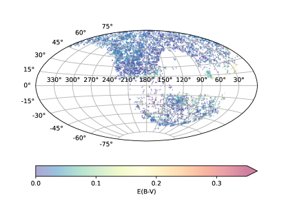
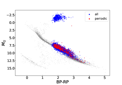
Figure 1: Top panel: Galactic distribution of the sample stars. The color bar means the extinction value. Bottom panel: Hertzsprung–Russell diagram of all sample. Blue points means all sample, red points means the sample with period. The grey points are the stars from Gaia eDR3 with distances $d<$ 200 pc, $G_{\rm mag}$ between 4–18 mag, and Galactic latitude —$b$— $>$ 10. No extinction was corrected for these stars.

Figure 2: Histograms of temperature (Panel a) and distance (Panel b) for the all dwarfs and the periodic stars. Panel b also plots the distance distributions of M0–M3 and M4–M7 dwarfs. The vertical line marks a distance of 100 pc.

Figure 2 shows the histograms of the effective temperature and distance for the sample stars, and Table 2 shows the parameters of the stars. The periodic sample refers to stars with rotational period estimations (Section 3.3).

3 Magnetic activity of M-type stars

3.1 UV activity indices

The definition of UV activity index is as following (Findeisen et al., 2011; Stelzer et al., 2013; Bai et al., 2018),

$$R^{\prime}_{\rm UV}=\frac{f_{\rm UV,exc}}{f_{\rm bol}}=\frac{f_{\rm UV,obs}\times(\frac{d}{R})^{2}-f_{\rm UV,ph}}{f_{\rm bol}}$$ (3)

where “UV” stands for the NUV and FUV bands, respectively. The superscript (^′) means that the the UV emission from photosphere has been subtracted. The $f_{\rm UV,exc}$ is the UV excess flux attributed to magnetic activity; $f_{\rm UV,obs}$ is the extinction-corrected flux inferred from the observed FUV or NUV magnitudes and extinction values; $f_{\rm UV,ph}$ is the photospheric flux from the stellar surface derived from stellar models; $f_{\rm bol}$ is the bolometric flux calculated from effective temperatures following $f_{\rm bol}=\sigma_{B}T^{4}_{\rm eff}$.

We estimated the extinction-corrected UV flux following

$$\begin{split}f_{\rm FUV,obs}=10^{-0.4\times(m_{\rm FUV}-18.82-R_{\rm FUV}\times E(B-V))}\\ \times 1.4\times 10^{-15}\times\delta\lambda_{\rm FUV}\end{split}$$ (4)

and

$$\begin{split}f_{\rm NUV,obs}=10^{-0.4\times(m_{\rm NUV}-20.08-R_{\rm NUV}\times E(B-V))}\\ \times 2.06\times 10^{-16}\times\delta\lambda_{\rm NUV},\end{split}$$ (5)

where $m_{\rm\lambda}$ is the observed magnitude from GALEX catalog, and $\delta\lambda_{\rm FUV}$ and $\delta\lambda_{\rm NUV}$ are the effective bandwidths of the FUV (442 Å) and NUV (1060 Å) filters, respectively (Morrissey et al., 2007; Findeisen et al., 2011). The extinction coefficients for FUV and NUV bands were calculated as 8.11 and 8.71 according to Cardelli et al. (1989). The reddening $E(B-V)$ was derived from the Pan-STARRS DR1 (PS1) 3D dust map (Green et al., 2015) with $E(B-V)=0.884\times{\rm Bayestar19}$. For sources without extinction estimation from the PS1 dust map, we used the SFD dust map (Schlegel et al., 1998) with $E(B-V)=0.884\times E(B-V)_{\rm SFD}$ as a complement and only kept the sources with $E(B-V)$ $<$ 0.1.

The photospheric flux density from stellar surface was derived using BT-Settl (AGSS2009) stellar spectra models. The models include a 11-point grid of metallicities, with [Fe/H]= -4, $-$3.5, $-$3, $-$2.5, $-$2, $-$1.5, $-$1, $-$0.5, 0, 0.3, 0.5. For each star, we first selected the models with two closest metallicities, and then extracted the best model by comparing the observed and theoretical log$T_{\rm eff}$ and log$g$ values for each metallicity. With the flux densities given by each model, we obtained the final flux density by linear interpolation using metallicity. The photospheric flux was calculated by multiplying the flux density (in unit of erg/cm²/s/Å) with $\delta\lambda_{\rm UV}$ mentioned above.

The stellar radius was calculated from observed 2MASS ($J$, $H$, and $K_{\rm S}$) magnitudes, distance, extinction, and bolometric correction (BC):

$$\begin{split}R&=\sqrt{\frac{L_{\rm bol}}{4\pi\sigma_{B}T^{4}}}\\ &=\sqrt{\frac{10^{(-0.4\times(M_{\rm bol}-M_{\odot}))}L_{\odot}}{4\pi\sigma_{B}T^{4}}}\\ &=\sqrt{\frac{10^{(-0.4\times(m_{\rm\lambda}-5{\rm log}d+5-A_{\rm\lambda}+BC-M_{\odot}))}L_{\odot}}{4\pi\sigma_{B}T^{4}}},\end{split}$$ (6)

where $M_{\odot}$ is solar bolometric magnitude (4.74 mag) and $L_{\odot}$ is solar bolometric luminosity (3.828$\times 10^{33}$ erg/s). $m_{\rm\lambda}$ is the apparent magnitude of $J$, $H$, and $K_{\rm S}$ bands, respectively. The extinction $A_{\rm\lambda}$ is calculated as $A_{\lambda}=R_{\lambda}\times E(B-V)$, with the extinction coefficients estimated from Cardelli et al. (1989). The BC was derived using the isochrones Python module (Morton, 2015), with the stellar temperature, surface gravity, metallicity as inputs. The final radius is obtained as the average value of the radii derived from different bands. The results of the activity indices calculation are shown in Table 3.

The $\delta\lambda_{\rm FUV}$ and $\delta\lambda_{\rm NUV}$ in Eq. 4 and 5 are 442 Å and 1060 Å, respectively (Morrissey et al., 2007; Findeisen et al., 2011). We noticed that some studies estimated UV flux using narrower bandwidths, specifically $\delta\lambda_{\rm FUV}=268$ Å and $\delta\lambda_{\rm NUV}=732$ Å (Stelzer et al., 2013; Bai et al., 2018). In the latter case, both the observed flux and the photospheric flux decrease, leading to smaller activity indices (i.e., a reduction of $\approx$0.2 in $R^{\prime}_{\rm FUV}$ and $\approx$0.16 in $R^{\prime}_{\rm NUV}$).

3.2 Chromospheric activity indices

3.2.1 Ca II H$\&$K activity index

We calculated the S-index and then obtained the Ca II H$\&$K activity index $R^{\prime}_{\rm{HK}}$ using the low-resolution spectra from LAMOST DR9.

We calculated the S-index and $R^{\prime}_{\rm HK}$ based on Yang et al. 2023 (in prep.). Here we give a brief description of the method. The LAMOST S-index ($S_{\rm LAMOST}$) can be written as (Lovis et al., 2011; Karoff et al., 2016; Astudillo-Defru et al., 2017)

$$S_{\rm LAMOST} =8\alpha\cdot\frac{\Delta\lambda_{\rm H}}{\Delta\lambda_{\rm R}}\cdot\frac{\tilde{f}_{\rm H}+\tilde{f}_{\rm K}}{\tilde{f}_{\rm V}+\tilde{f}_{\rm R}}$$ (7)

$$=8\alpha\cdot\frac{1.09\rm\AA}{20\rm\AA}\cdot\frac{\tilde{f}_{\rm H}+\tilde{f}_{\rm K}}{\tilde{f}_{\rm V}+\tilde{f}_{\rm R}}$$

where $\tilde{f}_{\rm H},\tilde{f}_{\rm K},\tilde{f}_{\rm V},\tilde{f}_{\rm R}$ are the mean flux per wavelength interval in four bandpasses, and the correction factor $\alpha$ is 2.4 (Duncan et al., 1991).

A linear calibrating equation between $S_{\rm LAMOST}$ and the Mount Wilson Observatory scale ($S_{\rm MWO}$) was derived through the common stars of the LAMOST spectra and Boro Saikia et al. (2018), which was found (Yang et al. 2023, in prep.) to be

$$S_{\rm MWO} =a\cdot S_{\rm LAMOST}+b$$ (8)

$$a =2.89^{+0.21}_{-0.17}$$

$$b =-0.65^{+0.18}_{-0.20}$$

We then converted the calibrated S-index to $R^{\prime}_{\rm HK}$ following the relation in terms of the color index $B-V$ (see Astudillo-Defru et al., 2017, for more details), while the $B-V$ index was derived from effective temperature and metallicity based on the Dartmouth Stellar Evolutionary Database (Dotter et al., 2008).

3.2.2 $\rm H\alpha$ activity index

We calculated the stellar activity index $R^{\prime}_{\rm{H\alpha}}$ with $\rm{H\alpha}$ equivalent width (EW) using the LAMOST DR9 low-resolution spectra. $R^{\prime}_{\rm{H\alpha}}$ is the normalized $\rm{H\alpha}$ luminosity defined as (Walkowicz et al., 2004)

$$R_{\rm{H\alpha}}^{{}^{\prime}}=\chi\times\rm{EW}^{{}^{\prime}}.$$ (9)

Here $\rm{EW}^{\prime}$ is the EW caused by dynamo-driven magnetic activity, which was calculated as follows,

$$\rm{EW}^{\prime}=\rm{EW}-\rm{EW}_{\rm{basal}},$$ (10)

where

$$\rm{EW}_{\rm{H\alpha}}=\int\frac{\emph{F}_{\rm{c}}-\emph{F}_{\rm{\lambda}}}{\emph{F}_{\rm{\lambda}}}.$$ (11)

$\rm{EW}_{\rm{basal}}$ represents the $\rm{H\alpha}$ emission due to physical processes unrelated to magnetic activity. The basal flux of $\rm{H\alpha}$ was derived through fitting a spline function to the $EWs$ of the most inactive stars in our sample.

The normalized factor $\chi$ was estimated following (Han et al., 2023)

$$\chi=\frac{f_{\rm{\lambda}6564}}{f_{\rm{bol}}}=\frac{f_{\rm{\lambda}6564}}{\sigma_{B}T^{4}},$$ (12)

where $f_{\rm{\lambda}6564}$ was the continuum flux at 6564 Å, which was derived through fitting the continuum of PHOENIX model spectrum (Husser et al., 2013) corresponding to the stellar parameters of our targets, and $f_{\rm{bol}}$ was the bolometric flux on stellar surface (for more details refer to Han et al., 2023).

3.3 Rotation periods and Rossby number

We first collected stellar rotation periods from previous photometric surveys, including Kepler/K2, ASAS-SN, ZTF, etc. The rotation periods of 199, 48, 76, 259 and 1 stars were obtained from the K2, ZTF, ASAS-SN, TESS and HATNet data, respectively. For these sources, we downloaded the photometric data and and visually checked the phase-folded light curves. Next, we cross-matched our sample with the TESS archive data, downloaded the light curve data, and estimated the rotation periods using the Lomb-Scargle method (VanderPlas, 2018). The phase-folded curves were checked by eye as well. Our period estimations are in agreement with those from Newton et al. (2016) and Fetherolf et al. (2022), indicating the reliability of our period determination, although some periods given by Hartman et al. (2011) are doubled compared with our estimations (Figure 3).

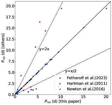
Figure 3: Comparison between the periods from TESS light curve data (in this paper) and the periods derived from previous studies. The blue points are the periods from Fetherolf et al. (2023), the red points are the periods from Hartman et al. (2011), and the green points are the periods from Newton et al. (2016). The black line is y=x, and the black dashed lines are y=2x and y=x/2, respectively.

The Rossby number is usually used to trace the stellar rotation, which is defined as the ratio of the rotation period to the convective turnover time (Ro $=$ P/$\tau$). We obtained the $\tau$ value using a grid of stellar evolution models from the Yale-Potsdam Stellar Isochrones (YaPSI; Spada et al., 2018) following Wang et al. (2020). Here we used the effective temperature $T_{\rm eff}$ and bolometric luminosity $L_{\rm bol}$ to fit the model evolutionary tracks. For each star, we obtained best-fit models for close metallicities, and calculated the final $\tau$ value by linear interpolation to the metallicity. The period, convective turnover time and Rossby number of stars are shown in Table 4. Note that compared with the classical empirical estimate of $\tau$ (Noyes et al., 1984), the ratio between the $\tau$ from theoretical YAPSI model and empirical $\tau$ values are around 3 (Wang et al., 2020).

3.4 Activity-rotation relationship

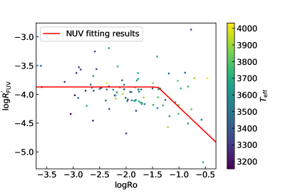
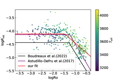
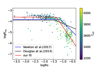
Figure 4: The activity-rotation relation of the GAELX NUV band (Panel a), FUV band (Panel b), Ca II H$\&$K line (Panel c), and H$\alpha$ line (Panel d), respectively. The points means the periodic sample, and the color bar represent the effective temperature. The black and purple line in Panel (c) correspond to the findings reported in Boudreaux et al. (2022), and Astudillo-Defru et al. (2017), respectively, but they have been horizontally shifted to the left by a factor of $\rm Ro/3$. The blue and black line in Panel (d) are from Newton et al. (2017) and Douglas et al. (2014), respectively, but shifted to left with a ratio of $\rm Ro/3$. The red line represent the fitting result from our sample.

For the UV and chromospheric activity indices, we performed a piecewise fitting analysis to study the activity-rotation relationship following

$$R^{\prime}_{\rm\lambda}=\begin{cases}R^{\prime}_{\rm\lambda,sat},\quad\rm if\ Ro\leq\rm Ro_{sat}\\ C\times\rm Ro^{\beta},\quad\rm if\ Ro>\rm Ro_{sat}.\end{cases}$$ (13)

Here $\lambda$ indicates the activity indices of NUV, FUV, $\rm H\alpha$ and Ca II H$\&$K lines.

Figure 4 shows the fitting result for the NUV band, with log$R^{\prime}_{\rm NUV,sat}=-3.50\pm 0.02$, log$\rm Ro_{sat}=-1.40\pm 0.05$ and $\beta=-0.87\pm 0.07$ (Table 1). Due to the limited number of samples with FUV observations, we did not directly perform a fitting analysis for the FUV band. However, we can derive the activity-rotation relation for FUV band by fitting a relation between $R^{\prime}_{\rm FUV}$ and $R^{\prime}_{\rm NUV}$. As shown in Figure 5, there is a linear relationship between log$R^{\prime}_{\rm NUV}$ and log$R^{\prime}_{\rm FUV}$, which can be quantified as follows,

$${\rm log}R^{\prime}_{\rm FUV}=(1.07^{+0.02}_{-0.02})\times{\rm log}R^{\prime}_{\rm NUV}-(0.16^{+0.06}_{-0.06})$$ (14)

The fitting result slightly differs from the result given by Stelzer et al. (2013). We found the larger slope ($\approx$1.3) reported by Stelzer et al. (2013) is mainly caused by the M stars in the TW Hya association, which clearly shows a deviation in the $R_{\rm UV}$ with their 10 pc sample (see their Figure 14). The relation between the FUV activity and rotation can then be described as log$R^{\prime}_{\rm FUV,sat}=-3.87\pm 0.02$, log$\rm Ro_{sat}=-1.40\pm 0.05$ and $\beta=-0.87\pm 0.07$.

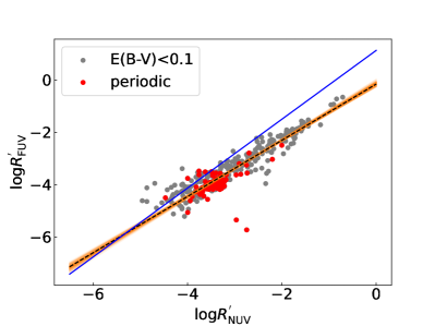
Figure 5: The compare of $R^{\prime}_{\rm NUV}$ and $R^{\prime}_{\rm FUV}$ in log-log scale. The gray points are the stars that E(B-V) less than 0.1, and the red points are the periodic sample. The black dashed line is the MCMC fitting result. The blue line is the results from Stelzer et al. (2013).

Figure 4 shows the relation between log$R^{\prime}_{\rm{HK}}$ and $\rm Ro$. We fitted the relation using Equation 13 and obtained the parameters as log$R^{\prime}_{\rm{HK,sat}}=-4.11\pm 0.02$, log$\rm Ro_{sat}=-1.47\pm 0/05$, and $\beta=-0.73\pm 0.06$. The $\beta$ value is in good agreement with that from Lehtinen et al. (2020) ($\beta\approx-0.97$), who studied the Ca II H$\&$K activity of F, G, and K type stars. The log$R^{\prime}_{\rm{HK,sat}}$ is notably higher than the value reported by Boudreaux et al. (2022), but very similar to Astudillo-Defru et al. (2017). The log$\rm Ro_{sat}$ and $\beta$ values are different with those values from Astudillo-Defru et al. (2017) and Boudreaux et al. (2022). One explanation is that there are very few sources located in the transition region in their sample, and the choice of the knee point greatly affects the slope in the unsaturated region. In addition, although our sample has a larger number, there are also many scatters, which would affect the accuracy of the fitting results.

Figure 4 shows the best-fit result with log$R^{\prime}_{\rm H\alpha,sat}=-3.63\pm 0.03$, log$\rm Ro_{sat}=-1.35\pm 0.03$ and $\beta=-2.52\pm 0.14$. The $\beta$ value is different with previous studies, e.g., $\beta=-1.7\pm 0.1$ from Newton et al. (2017) or $\beta=-0.73^{+0.16}_{-0.12}$ from Douglas et al. (2014). In the unsaturated region, both of their samples have many sources with lower activity indices (log$R^{\prime}_{\rm H\alpha}\approx-6$) which do not match their relations. We tried to perform a fitting including these sources and derived a larger slope. The slight difference of log$R^{\prime}_{\rm H\alpha,sat}$ is likely due to the different calculation method of the normalized factor $\chi$. Moreover, Douglas et al. (2014) studied a mono-age population and didn’t correct for baseline. All these may result in some differences in the activity distributions and fitted relations.

Table 1: The fitting results of the activity-rotation relations for four proxies.

band	log$R^{\prime}_{\rm\lambda,sat}$	log$\rm Ro_{sat}$	$\beta$
NUV	$-3.50\pm 0.02$	$-1.40\pm 0.05$	$-0.87\pm 0.07$
FUV	$-3.87\pm 0.02$	$-1.40\pm 0.05$	$-0.87\pm 0.07$
Ca II H$\&$K	$-4.11\pm 0.02$	$-1.47\pm 0.05$	$-0.73\pm 0.06$
$\rm H\alpha$	$-3.63\pm 0.03$	$-1.35\pm 0.03$	$-2.52\pm 0.14$

3.5 Distribution of stellar activity indices

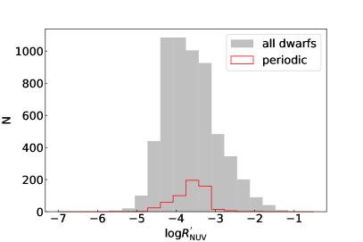
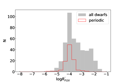
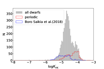
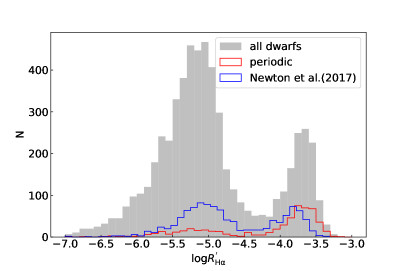
Figure 6: Histogram of log$R^{\prime}_{\rm NUV}$ (Panel a), log$R^{\prime}_{\rm FUV}$ (Panel b), log$R^{\prime}_{\rm HK}$ (Panel c) and log$R^{\prime}_{\rm H\alpha}$ (Panel d). The gray filled bars represent the all dwarfs and the red line represent the periodic stars. The blue line in Panel c and d is the distribution of log$R^{\prime}_{\rm H\alpha}$ and log$R^{\prime}_{\rm HK}$ for M stars from Newton et al. (2017) and Boro Saikia et al. (2018), respectively.

Figure 6 shows the distributions of $R^{\prime}_{\rm NUV}$, $R^{\prime}_{\rm FUV}$, $R^{\prime}_{\rm HK}$, and $R^{\prime}_{\rm H\alpha}$.

There is a wide distribution value of log$R^{\prime}_{\rm NUV}$ ($\sim$ $-5$ to $-$2) and log$R^{\prime}_{\rm FUV}$ ($\sim$ $-5$ to $-$1). Considering that the saturation regime for the UV bands are log$R^{\prime}_{\rm NUV}$ $\approx$ $-$3.5 and log$R^{\prime}_{\rm FUV}$ $\approx$ $-$3.9, the stars with quite high activity (log$R^{\prime}_{\rm UV}$ $\gtrsim$ $-$2.5) may be due to some contamination (see detailed discussion in Section 3.6).

There is a noticeable gap in the activity distribution of $\rm H\alpha$ and Ca II H$\&$K emission, similar to the Vaughn–Preston gap (Vaughan & Preston, 1980) discovered for F and G stars. Possible explanations include sample incompleteness or a fast transition between the two populations. The scenario of sample incompleteness can be ruled out since many previous studies (Newton et al., 2016; Magaudda et al., 2020; Santos et al., 2020; Boudreaux et al., 2022; Han et al., 2023), using different samples and activity proxies, have also reported a similar double-peaked distribution for M stars. The double peaks are quite consistent with the saturated region (log$R^{\prime}_{\rm{HK}}\approx-4$; log$R^{\prime}_{\rm H\alpha}\approx-3.5$) and the unsaturated region (log$R^{\prime}_{\rm{HK}}\approx-5$; log$R^{\prime}_{\rm H\alpha}\approx-5$). Therefore, this gap is most likely due to a transition from the fast-rotating saturated population to the slow-rotating unsaturated population (Newton et al., 2016; Stelzer et al., 2016; Boudreaux et al., 2022), which suggests a lack of stars with intermediate rotational periods and thus a discontinuous spin-down evolution (Magaudda et al., 2020).

In order to investigate above scenario, we further examined the distribution of rotation periods $P_{\rm rot}$ and three galactic orbital parameters, including the vertical action $Jz$, maximum vertical height $zmax$, and eccentricity $e$ (Figure 7). These orbital parameters were measured with the $galpy$ package (Bovy, 2015), under the Stäckel approximation (Binney, 2012) with the Milky Way potential MWPotential2014. The clear difference in the rotation periods between the two populations (Figure 7, Panel a) suggests that the scenario is plausible. A rapid decay of the rotation period during a stage of stellar evolution leads to a significant weakening of stellar activity. The three orbital parameters, which are approximate indicators of stellar age, indicate that the saturated population are generally (dynamically) younger than the unsaturated one, which is consistent with previous studies (Irwin et al., 2011; West et al., 2015; Newton et al., 2016). In addition, such a double-peaked distribution exists from M0 to M4 types, it is unlikely that the two populations are caused by distinct magnetic dynamos, such as the tachocline ($\alpha$–$\Omega$) and convective ($\alpha^{2}$) dynamos.

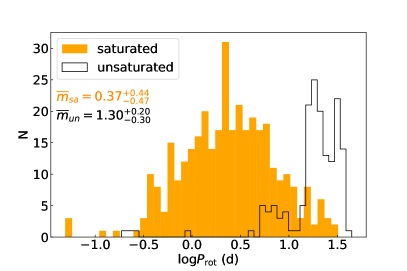
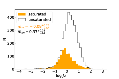
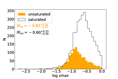
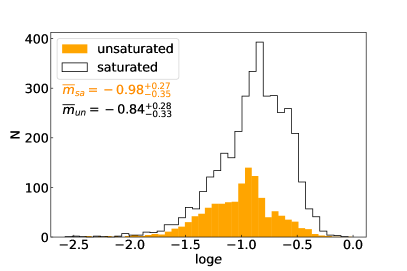
Figure 7: Histogram of period (Panel a), $Jz$ (Panel b), $zmax$ (Panel c) and eccentricity (Panel d). The x-axis is the log scale. The orange filled bars represent the unsaturated stars (log$R^{\prime}_{\rm H\alpha}<-4.5$) and the black line represent the saturated stars (log$R^{\prime}_{\rm H\alpha}\geq-4.5$). The $\bar{m}_{un}$ and the $\bar{m}_{sa}$ represent the median value for the unsaturated sample and saturated sample, respectively.

The distribution reveals a clear evolution from M0 to M6 types (Figure 8 and Figure 9): (1) for M0 and M1 types, most stars reside in the unsaturated region, and the double-peaked feature is weak for the Ca II H$\&$K band; (2) for M2 to M4 types, the portion of saturated and unsaturated population are approximately equal; (3) for M5 and M6 types, the distribution evolves into a single peak located in the saturated region, with only a few stars ($\lesssim$10%) remaining in the unsaturated region. This can be explained by that different topology of magnetic fields results in various stellar winds and angular momentum losses, leading to diverse spin-down rates (Matt et al., 2012; Garraffo et al., 2015). The multipole magnetic field has a weaker magnetic breaking effect compared to a dipolar magnetic field, resulting in a more slowly decay of rotation in late-type M stars compared to early-type M stars (Matt et al., 2015). This also means both early-type (partly convective) stars and late-type (fully convective) stars operate rotation-dependent dynamos. Furthermore, the smooth evolution of the distribution from M0 to M6 subtypes imply a common dynamo for all the stars, in which the differential rotation and convection play more significant roles than the tachocline (Wright & Drake, 2016). It’s worth exploring whether the abrupt variation of activity from mid-type (M2–M4) to late-type (M5–M6) stars (Figure 8) is due to sample incompleteness (i.e., limited detection of very cool stars) or the operation of a distinct dynamo mechanism working for late-type stars.

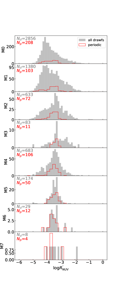
Figure 8: Number distribution of log$R^{\prime}_{\rm NUV}$ (Panel a) and log$R^{\prime}_{\rm FUV}$ (Panel b) for stars from M0 to M7. The gray filled bars represent the main-sequence stars, the red line represent periodic sample.

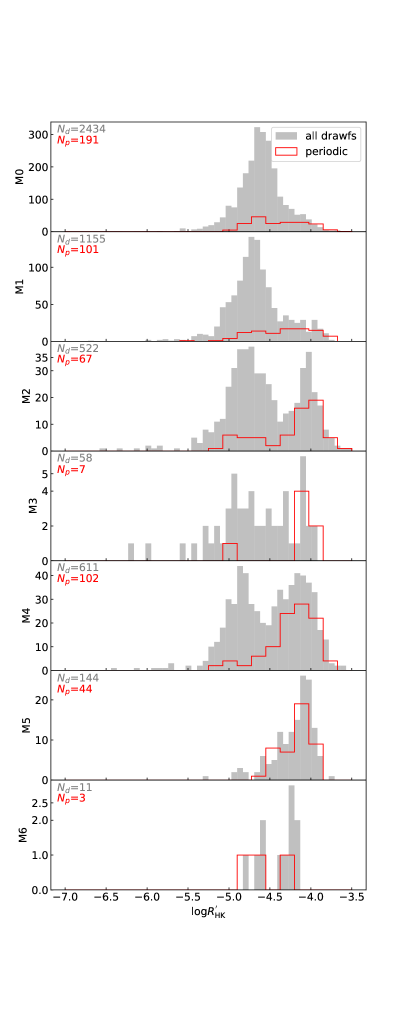
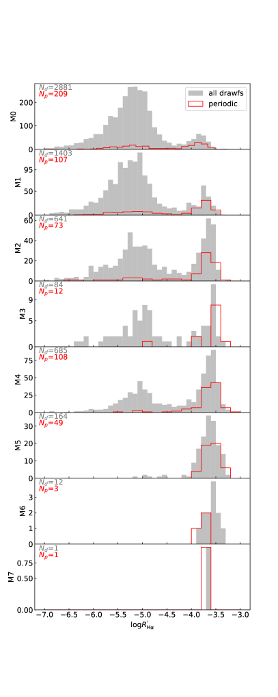
Figure 9: Number distribution of log$R^{\prime}_{\rm HK}$ (Panel a) and log$R^{\prime}_{\rm H\alpha}$ (Panel b) for stars with different subtypes. The gray filled bars represent the main-sequence stars, and the red line represent the periodic sample.

Table 2: Stellar parameters of the sample sources. $m_{\rm NUV}$ and $m_{\rm FUV}$ are the observed magnitude for GALEX NUV and FUV bands.

Gaia id	RA.	DEC.	$T_{\rm eff}$	log$g$	[Fe/H]	Distance	E(B-V)	$m_{\rm NUV}$	$m_{\rm FUV}$
3204245546431688192	64.22870	-3.16353	4024.66	5.07	-0.28	251.17	0.05	18.31	18.36
4437528912804247680	242.10202	4.60833	3901.46	5.09	-0.21	200.81	0.05	22.52	23.35
2485413805153218048	20.97025	-1.42260	3864.15	5.12	-0.18	531.54	0.05	21.44	22.88
919952552803891072	116.28023	38.00565	3830.86	5.06	-0.21	390.81	0.05	23.77	24.16
2807530137536007680	8.06760	25.40596	3925.00	4.97	-0.38	245.17	0.03	19.16	19.61
136899784754020224	44.58209	33.72791	3914.89	5.12	-0.36	313.34	0.10	19.89	20.94
931687674766627200	125.17405	48.30424	3864.97	5.02	-0.31	275.03	0.06	19.32	19.62
3702591288979144192	192.98948	2.01242	3888.94	4.90	-0.58	240.49	0.04	22.58	22.93
2645837194505938432	351.61309	2.03311	3671.00	4.61	-0.60	264.04	0.01	20.09	20.40
888816067133565056	102.74665	30.70783	3880.45	5.10	-0.20	361.34	0.06	21.82	22.55
663532010117882240	123.94805	19.55912	3848.31	4.90	-0.31	366.63	0.05	22.19	23.57
3267315693766344704	47.25408	1.82766	4015.03	5.50	0.25	565.48	0.11	20.66	21.70
3842831106588491008	136.54439	-0.16756	3678.77	4.89	-0.41	227.27	0.02	23.00	23.52
800590429486863104	144.42856	37.71175	3904.64	5.02	-0.28	312.39	0.05	20.77	21.96
342617001561387904	27.75182	37.22069	3755.53	4.95	-0.35	191.36	0.03	21.90	21.81
17728461062321536	51.40735	13.77185	3896.48	4.98	-0.32	301.21	0.27	19.02	18.53
1591488350438997632	221.87057	48.69225	4030.27	5.09	-0.33	288.57	0.04	18.89	19.09
661934557160165376	132.71120	21.36956	3860.80	4.97	-0.36	322.04	0.04	23.64	23.81
3646602125373348864	213.76290	-2.38854	3755.62	4.68	-0.79	303.94	0.07	22.70	23.38
3647017951221678976	212.87110	-2.30502	4018.31	5.17	-0.17	189.02	0.07	23.36	23.35

NOTE. (This table is available in its entirety in machine-readable and Virtual Observatory (VO) forms in the online journal. A portion is shown here for guidance regarding its form and content.)

Table 3: Stellar activity indices of the NUV, FUV, Ca II H$\&$K and $\rm H\alpha$ bands of the total sample.

Gaia id	log$R^{\prime}_{\rm NUV}$	log$R^{\prime}_{\rm FUV}$	log$R^{\prime}_{\rm HK}$	log$R^{\prime}_{\rm H\alpha}$
2772804845911842944	$-4.12\pm 0.03$	$-4.93\pm 0.12$	$-4.31\pm 0.01$	$-4.71\pm 0.07$
710834787049323392	$-3.37\pm 0.05$	$-3.92\pm 0.19$	$-3.83\pm 0.10$	$-3.72\pm 0.12$
680846672554039936	$-3.39\pm 0.03$	$-3.85\pm 0.14$	$-3.79\pm 0.20$	$-3.60\pm 0.29$
3146147042781951744	$-3.46\pm 0.03$	$-4.05\pm 0.16$	$-4.02\pm 0.01$	$-3.80\pm 0.05$
4413290007171520768	$-4.13\pm 0.03$	$-4.85\pm 0.18$	$-4.50\pm 0.01$	$-4.63\pm 0.13$
3367511306484702592	$-3.41\pm 0.05$	$-3.78\pm 0.16$	$-4.02\pm 0.02$	$-3.90\pm 0.07$
136899784754020224	$-2.00\pm 0.02$	$-2.50\pm 0.08$	$-4.05\pm 0.09$	$-3.94\pm 0.28$
1038927991625880832	$-4.06\pm 0.01$	$-5.22\pm 0.14$	$-4.42\pm 0.01$	$-5.45\pm 0.52$
578274091791263104	$-3.37\pm 0.01$	$-4.14\pm 0.09$	$-4.41\pm 0.02$	$-3.87\pm 0.04$
1303190835359164416	$-3.57\pm 0.03$	$-4.57\pm 0.15$	$-3.97\pm 0.01$	$-4.08\pm 0.06$
3809500549759137152	$-3.70\pm 0.01$	$-4.49\pm 0.13$	$-4.18\pm 0.02$	$-3.93\pm 0.03$
312984407278269568	$-3.31\pm 0.10$	$-3.46\pm 0.21$	$-4.31\pm 0.01$	$-4.46\pm 0.09$
663532010117882240	$-2.73\pm 0.03$	$-3.34\pm 0.17$	$-4.89\pm 0.01$	$-4.99\pm 0.79$
2593114821680113536	$-3.54\pm 0.01$	$-4.16\pm 0.08$	$-3.93\pm 0.06$	$-3.75\pm 0.10$
673218020362903040	$-3.57\pm 0.13$	$-3.65\pm 0.21$	$-4.10\pm 0.03$	$-3.91\pm 0.16$
3844876610533210496	$-3.68\pm 0.02$	$-4.46\pm 0.10$	$-4.34\pm 0.02$	$-4.30\pm 0.04$
100307419305322496	$-3.27\pm 0.05$	$-3.81\pm 0.14$	$-3.68\pm 0.05$	$-3.38\pm 0.02$
685749635420118912	$-3.80\pm 0.03$	$-4.26\pm 0.18$	$-4.87\pm 0.01$	$-4.95\pm 0.87$

NOTE. (This table is available in its entirety in machine-readable and Virtual Observatory (VO) forms in the online journal. A portion is shown here for guidance regarding its form and content.)

Table 4: The parameters of periodic sample.

Gaia id	Period	Ref.1	$\tau$	Ro
688528547980217088	17.96000	1	88.71	0.20
3132744335339029376	9.79997	4	82.72	0.12
740411679900325120	6.10162	4	94.51	0.06
740266991041907840	1.94940	3	96.13	0.02
5181296851945039360	10.64136	3	111.88	0.10
2481571802287972608	5.05442	4	86.33	0.06
2700541845063604992	0.76202	3	92.00	0.01
2651027782742343296	31.01000	1	105.75	0.29
3866696762383440256	18.80000	1	96.85	0.19
879903868258387968	17.96056	4	119.21	0.15
679329621385921536	1.20710	3	98.81	0.01
631716232416975488	17.07000	1	96.85	0.18
3146147042781951744	2.08639	4	97.23	0.02
638525198689503360	22.59000	1	109.31	0.21
1415189357506518272	8.88880	2	99.60	0.09
1325695295758670208	10.72802	4	107.98	0.10
222248893824346112	10.05350	4	109.91	0.09
127275106640433664	4.64074	4	104.41	0.04
1904506975722625408	6.67416	4	90.47	0.07
1896376289095348352	3.30535	4	102.00	0.03

Note. The references include 1: Reinhold & Hekker (2020) from K2 data; 2: Chen et al. (2020) from ZTF data; 3: Jayasinghe et al. (2020) and Christy et al. (2022) from ASAS-SN data; 4: Howard et al. (2022), Prsa et al. (2022) and our estimations from TESS data; 5: Newton et al. (2016) from HATNet data. (This table is available in its entirety in machine-readable and Virtual Observatory (VO) forms in the online journal. A portion is shown here for guidance regarding its form and content.)

3.6 Relation between different activity indices

Figure 10 (top panels) shows the comparison between log$R^{\prime}_{\rm{HK}}$ and log$R^{\prime}_{\rm NUV}$. There is a positive but scattered relation, and the scatter is mainly caused by some objects with high levels of UV emission, which may be influenced by their surrounding environments. The number of scatter points decreases for the sample with $E(B-V)<0.1$ and $SNR>30$ (middle panels). The stars with rotational period measurements (right panel) show a clear correlation between the two indices. A Markov Chain Monte Carlo (MCMC) fit was applied to these stars, and the result is

$${\rm log}R^{\prime}_{\rm{HK}}=0.44^{+0.04}_{-0.04}\times{\rm log}R^{\prime}_{\rm NUV}-2.68^{+0.14}_{-0.13}.$$ (15)

Figure 10 (middle panel) also shows a positive but diffuse relation between log$R^{\prime}_{\rm{H\alpha}}$ and log$R^{\prime}_{\rm NUV}$. The MCMC fitting result of the relation using the periodic sample is

$$\log R^{\prime}_{\rm{H\alpha}}=1.15^{+0.08}_{-0.07}\times\log R^{\prime}_{\rm NUV}-0.07^{+0.26}_{-0.27}.$$ (16)

There is a clear and tight relation between log$R^{\prime}_{\rm{H\alpha}}$ and log$R^{\prime}_{\rm HK}$, shown in Figure 10 (bottom panel). A linear fitting using the periodic sample gives

$$\log R^{\prime}_{\rm{H\alpha}}=1.88^{+0.06}_{-0.06}\times\log R^{\prime}_{\rm HK}+3.80^{+0.25}_{-0.26}.$$ (17)

Furthermore, we also did a piecewise fitting between the log$R^{\prime}_{\rm{H\alpha}}$ and log$R^{\prime}_{\rm HK}$ because they have two populations, and the fitting result is

$$\log R^{\prime}_{\rm{H\alpha}}=\begin{cases}(2.59\pm 0.15)\times\log R^{\prime}_{\rm HK}+(7.01\pm 0.27),\\ \quad{\rm if}\ \log R^{\prime}_{\rm HK}\leq\rm-4.26\pm 0.06\\ (1.06\pm 0.22)\times\log R^{\prime}_{\rm HK}+(0.53\pm 0.34),\\ \quad{\rm if}\ \log R^{\prime}_{\rm HK}>\rm-4.26\pm 0.06.\end{cases}$$ (18)

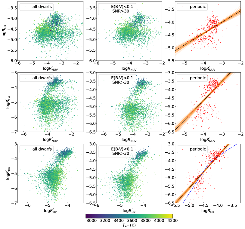
Figure 10: Top panels: Comparison of $R^{\prime}_{\rm NUV}$ and $R^{\prime}_{\rm{HK}}$. The samples from left to right panels are all dwarfs, targets with low extinction ($E(B-V)<0.1$) and high SNR (SNR $>$ 30), targets with period measurements. The black dashed line is the fitting result. Middle panels: Comparison of $R^{\prime}_{\rm NUV}$ and $R^{\prime}_{\rm H\alpha}$. Bottom panels: Comparison of $R^{\prime}_{\rm H\alpha}$ and $R^{\prime}_{\rm{HK}}$. The blue dashed line is the result from piecewise fitting.

We noticed a group about 400 stars (out of a total of 6629) show very high UV activity above the saturation value, characterized by log$R^{\prime}_{\rm UV}$ $\gtrsim$ $-$2.5 (hereafter “oversaturated”, also shown in Figure 8), while exhibiting low levels of chromospheric activity. Several studies (e.g., Shkolnik et al., 2011; Stelzer et al., 2013; Jones & West, 2016) have also identified groups of stars with high UV activity, but the underlying reason remains unknown. Figure 11 shows the spatial distribution and Toomre diagram of our sample stars. The majority of the population with high UV activity are located in the thin disk, like most of the sample stars. Generally, these objects have a more scattered distribution. When compared to stars with similar apparent magnitudes, these objects are notably positioned at larger distances from the galactic center and the galactic plane.

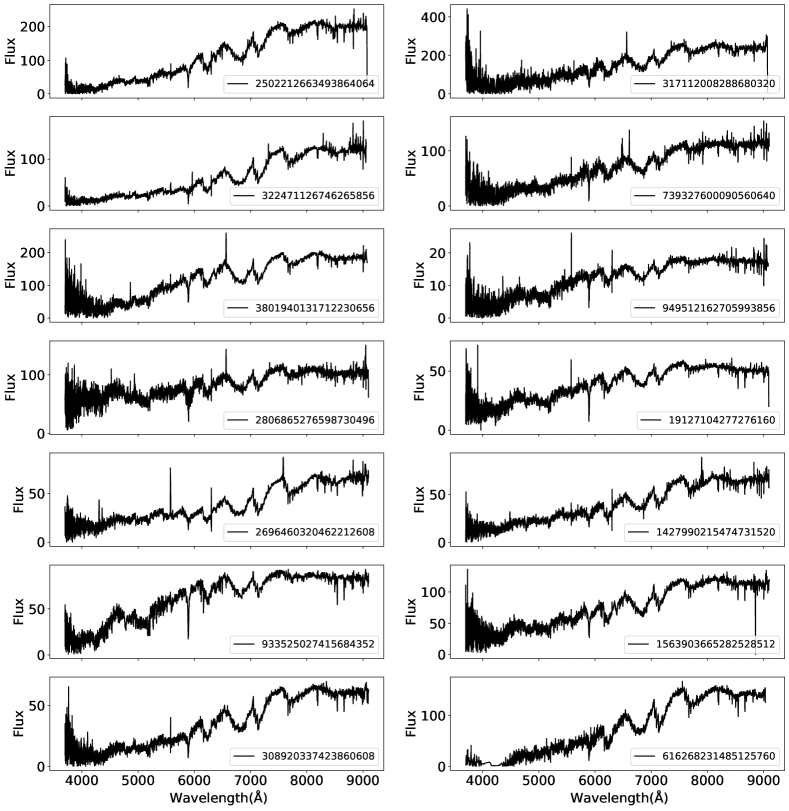
Figure A1: Examples of the LAMOST low-resolution spectra for stars with log$R^{\prime}_{\rm NUV}>-2.5$.

We considered several explanations including the presence of a white dwarf companion or a companion with a similar stellar type, contamination from surrounding environment, chance alignment with extragalactic sources, over-estimated extinction, or the possibility of a very young stellar population. First, we did not find any UV spectral observations (e.g., from Hubble or IUE) for these sources. By visually checking the LAMOST spectra of these stars, only 5% of them show a possible excess in the blue band (Figure A1). However, no wide Balmer absorption lines can be recognized. This suggests that the scenario involving a white dwarf companion can not be the main reason. Second, during the sample construction, we have employed a series of methods to identify and remove binaries. An examination of these stars on the HR diagram reveals that they do not fall within the binary belt, ruling out the scenario of a companion with a similar stellar type. Third, we checked the DSS and PanSTARRS images of these sources and found that none of them are located in a nebula or star-forming region. Forth, we cross-matched these sources with the GLADE+ galaxy catalog (Dálya et al., 2018) using match radii of 10/20/30 arcseconds, resulting in only 13/36/66 matches. This means the chance mismatch cannot account for the exceptionally active sample. Fifth, almost all of these stars have E(B-V) less than 0.1 and the extinction uncertainty is small ($\lesssim 0.03$). Despite the large UV extinction coefficient, extinction cannot be the main reason for the over-saturated stars. Fifth, almost all of these stars have $E(B-V)$ values less than 0.1, and their extinction uncertainties are small ($\lesssim 0.03$). Despite the large UV extinction coefficient, it is unlikely that extinction is the primary reason for the oversaturation of these stars. Finally, although young stars (with an age of several million years) could exhibit very high UV activity (Shkolnik & Barman, 2014; Schneider & Shkolnik, 2018), most of these sources have large values of $zmax$ and $J_{z}$, suggesting that they are dynamically old.

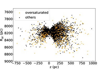
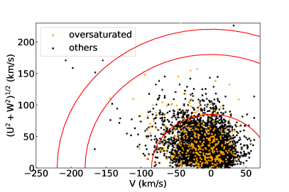
Figure 11: Galactic parameters of the oversaturated population (yellow points) and other stars (black points). Panel (a): Galactocentric distance versus the distance to the Galactic plane. Panel (b): Toomre diagram. The three red lines represent constant values of the total Galactic velocity of 85, 180, and 220 km/s (from bottom to top), respectively.

4 UV flare

We further searched for flare events using the GALEX data, since they are also good indicators of stellar activity. Firstly, we extracted the UV light curves of our targets using “gPhoton”, a software package that enables analysis of GALEX ultraviolet data at the photon level (Million et al., 2016). There are a total of 10211 FUV and NUV observations for the 6629 sources. Secondly, we tried to identify the flare events using the sigma clipping method, and a flare event was identified when three consecutive data points exhibited a flux higher than 3$\sigma$ (Yang & Liu, 2019). We also found that the FLAIIL pipeline (Loyd et al., 2018), which was developed for identifying flares in the FUV light curves from the MUSCLES data, is not suitable for many of our sources, due to that the exposure time is too short to establish the quiescent phase accurately. Thirdly, we visually checked the light curve with possible flare events, and threw away the fake identifications and incomplete flares. Finally we derived 43 complete flare events for 35 stars, which are listed in Table 5.

The durations of these flares range from $\approx$60 to $\approx$900 seconds, and the peak luminosities range from $10^{28}$ to $10^{31}$ erg/s. Most flares stars have subtypes ranging from M0 to M5. Figure 12 displays some flares with typical signatures (Welsh et al., 2007), including Type 1 flares (rapid rise and slow decay within 500 seconds) like 3836711087429390976, Type 2 flares (rapid rise and several peaks during the slow decay lasting longer than 500 seconds) like 1029095918132946176, and Type 3 flares (complicated shapes) like 2645345918966845440.

Table 5: All flare events in our sample.

Gaia id	Band	$\rm t_{\rm end}-t_{\rm start}$	Equivalent duration	Peak luminosity	Flare energy	log$R^{\rm\prime}_{\rm flare}$
		(s)	(s)	log (erg/s)	log (erg)
3836711087429390976	FUV	160	4039	30.59	31.86	-1.70
	NUV	294	5215	30.70	32.58
636520926431812096	FUV	364	1006	30.23	31.87	-2.16
	NUV	362	1361	30.40	32.39
1545784091618733184	FUV	252	778	30.10	31.31	-2.60
	NUV	282	1487	30.16	32.02
2645345918966845440	NUV	379	1957	28.93	30.96	-2.68
	NUV	900	14162	29.23	31.82
2485820216434079360	NUV	165	32	29.22	30.12	-1.90
	NUV	195	1815	30.37	32.01
1449481785146363648	FUV	476	747	30.23	31.59	-2.85
	NUV	285	595	30.13	31.78
	NUV	350	2012	30.47	32.37
855090094138137088	NUV	77	79	28.75	30.01	-2.49
	NUV	398	908	29.14	31.07
2645381962332324992	NUV	283	879	30.93	32.70	-1.75
2698395946257300992	FUV	408	784	30.28	31.72	-2.26
1287410781917419264	NUV	180	723	30.22	32.00	-2.34
1282550012807310976	FUV	284	279	30.64	31.19	-1.95
3851331671501030784	FUV	196	255	29.83	31.21	-2.62
3836050766272513408	NUV	253	290	30.67	32.39	-2.02
2550158684794063744	NUV	318	36	29.70	30.71	-3.09
2575639321307107328	FUV	299	385	30.06	31.27	-2.42
3665691266433813248	NUV	275	191	28.99	30.60	-3.12
698725624975112192	NUV	457	981	31.10	33.03	-1.81
1449480616915236864	NUV	315	1168	30.75	32.21	-1.80
2561205585492641280	FUV	401	291	30.07	31.43	-2.26
2679196892688576384	FUV	101	241	29.12	30.48	-2.99
2644562860529295872	NUV	177	309	30.32	32.11	-2.27
4014961305479623424	NUV	239	403	29.45	31.34	-2.65
700016245467419136	FUV	745	150	29.34	30.91	-3.03
3648394677218755584	NUV	218	2135	29.06	31.05	-2.52
2815503108666238464	NUV	464	1039	28.81	30.89	-2.86
1479643038364982528	NUV	64	68	30.00	30.89	-2.45
684640777943741568	NUV	322	447	29.96	31.87	-1.86
666154478491325440	NUV	281	1647	29.23	31.17	-2.72
742553498486917888	NUV	481	776	29.45	31.63	-2.25
735728623654810624	NUV	479	702	29.49	31.49	-1.77
658601456379862784	NUV	321	321	29.07	30.71	-2.30
659265630123576448	NUV	186	397	29.51	31.12	-2.19
3266937637860051840	NUV	311	3094	29.22	30.86	-1.64
1314209831654576768	FUV	254	317	32.72	34.28	-3.86

We calculated the energy of all flare events as follows (Jackman et al., 2023; Rekhi et al., 2023),

$$E=4\pi d^{2}\delta\lambda\int_{t_{\rm start}}^{t_{\rm end}}(F(t)-F_{0})dt,$$ (19)

where $d$ is the distance from Gaia eDR3, $\delta\lambda$ is the effective bandwidths of FUV and NUV bands, $t_{\rm start}$ and $t_{\rm end}$ are the times when the flare starts and ends, respectively. $F(t)$ is the measured flux at each time point during the flare, and $F_{0}$ is the estimated quiescent flux. We calculated the quiescent flux using an iterative method. First, the data point with the largest flux and adjacent points were removed. Then, two iterations were carried out to excluded the points with fluxes higher than 1$\sigma$. Finally, the median flux of the remaining points was calculated as the quiescent flux. The time corresponding to the first point with a flux larger than the quiescent flux marks the start of the flare ($t_{\rm start}$), and the time corresponding to the last point with a flux higher than the quiescent flux represents the end of the flare ($t_{\rm end}$). The flare energy ranges from $10^{30}$ to $10^{34}$ erg, similar to the range of optical flares (e.g., Yang et al., 2017). The flare activity index was calculated following $R^{\prime}_{\rm flare}=\frac{\Sigma E_{\rm flare}}{\int L_{\rm bol}dt}=\frac{\Sigma E_{\rm flare}}{L_{\rm bol}\times\Delta{t}}$ (Yang et al., 2017). Here $\Sigma E_{\rm flare}$ means the sum of the energy of all flare events for each source, and $\Delta{t}$ represents the total duration of these flares.

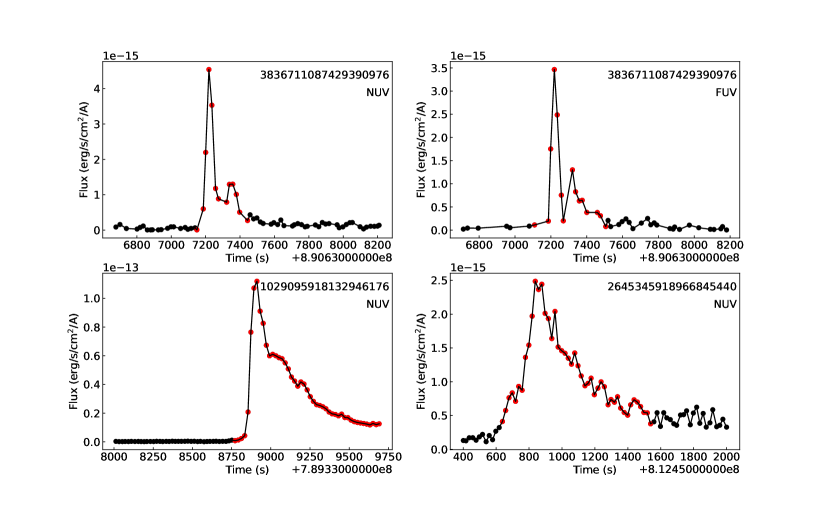
Figure 12: UV light curves of flare events. Upper panels: flare events observed simultaneously in the NUV and FUV bands for 3836711087429390976. Bottom panels: flares observed at different times in NUV band for 1029095918132946176 and 2645345918966845440. Black points are the quiescent state, red points are the flares.

5 Habitable Zone

The habitability of exoplanets around M dwarfs is quite worthy of investigation due to the abundance of M-type stars in the Milky Way and the the extensive existence of exoplanets expected orbiting them (Shields et al., 2016).

A planet was normally considered habitable when it resides in a region where suitable temperatures allow water to remain liquid on its surface. This habitable zone is mainly determined by the properties of the host star (e.g., luminosity, effective temperature) and the distance between the planet and the star. A continuously habitable zone (CHZ: Kasting et al., 1993; Kopparapu et al., 2013) was defined by establishing both an inner edge, calculated by the loss of water via photolysis and hydrogen escape, and an outer edge, determined by the maximum greenhouse due to $\rm CO_{2}$ clouds.

The habitable zone is also influenced by stellar magnetic activity, especially X-ray and UV emission and flares. Thus, the habitability of planets surrounding M-type stars has been a topic of long-standing debate (Shields et al., 2016). Although detailed effects of stellar activity on atmosphere of planets are not well understand, it has generally been believed that high activity (frequent flares and high levels of X-ray and UV activity) can be life-threatening, leading to atmospheric erosion (Sanz-Forcada et al., 2010) and damaging biomolecules (Sagan, 1973). On the contrary, some experimental studies (e.g., Toupance et al., 1977; Ritson & Sutherland, 2012; Patel et al., 2015) reported that UV emission can serve as a source of energy for prebiotic chemical synthesis, especially for ribonucleic acid (RNA), which is the building blocks for the emergence of life, while the low total UV emission of M stars may not support life processes like the chemical synthesis of complex molecules (Ranjan et al., 2017; Rimmer et al., 2018). Taking these arguments into consideration, the concept of an ultraviolet habitable zone (UHZ) can be defined.

The overlapping region between CHZ and UHZ can be considered as the most favorable for habitability. In this study, we first derived the CHZs for our sources using the method of Kopparapu et al. (2014). The inner edge of CHZ was calculated using the “runaway greenhouse” limit (i.e., greenhouse effect caused by water), and the outer edge was determined using the “maximum greenhouse” limit. For these calculations we assumed a planet mass equivalent to that of Earth. The CHZ was calculated following $d=(\frac{L/L_{\odot}}{S_{\rm eff}})^{0.5}$ AU (Kopparapu et al., 2014), where $S_{\rm eff}$ is the effective solar flux incident on the planet. Then the UHZ was defined following Spinelli et al. (2023): the outer boundary of the UHZ was established with $f_{\rm UV}\geq$ 45 erg cm^-2 $s^{-1}$, and the inner boundary was set with $f_{\rm UV}\leq$ 1.04$\times 10^{4}$ erg cm^-2 $s^{-1}$, twice the intensity of UV radiation that the Archean Earth received 3.8 billion years ago.

Figure 13 shows the NUV luminosity $L_{\rm NUV}$ versus the star–planet distance $a$. The lower and upper black lines represent the inner and outer boundaries of the UHZ, respectively. The orange lines represent the CHZs for each target. Furthermore, we divided these stars into different bins based on their NUV luminosities. For each bin, an conservative CHZ (dark blue shaded area) was calculated from the median values of the inner edges and the outer edges of the CHZs of each target. Additionally, a more optimistic CHZ (light blue shaded area) was derived from the combination of the 16% to 84% values of the inner edges and the outer edges of the CHZs for each star. The samples shown from the top panel to the bottom panel are M dwarfs within 100 pc, stars with rotational periods, and the total sample. Table 6 presents the probability of habitability for different samples. Specifically, for nearby M stars within 100, 50, and 25 pc—a closer distance suggests a more complete sample, about 44%, 42%, and 41% respectively, exhibit overlapping CHZ and UHZ regions. Our results suggest for a significant number of M dwarfs, planets situated in the overlapping CHZ and UHZ regions are likely to be habitable.

We further examined the impact of stellar UV variability on its habitability. We downloaded the data from multiple observations in the GALEX $VisitPhotoObjAll$ catalog using a match radius of 3$\arcsec$ via the CasJobs. This led to 3804 stars with multiple observations, with observation time spanning from 0.01 day to 9 years. We replaced the NUV flux with the lowest and highest fluxes in multiple observations to access whether any of these stars would move outside the range of UHZ. We found that around 0.31% stars shifted outside the UHZ range. In addition, for the stars with UV flares, we calculated used the peak luminosities during the flare events. Even we use the peak luminosity as the normal UV luminosity, most stars are still located in the UHZ region (Figure 14). In summary, UV variation had little impact on the probability of stellar habitability.

Table 6: The number of stars and probability of habitability for different samples. N: The total number of stars. P1: Probability of habitability by selecting star with overlapped CHZ and UHZ. P2: Probability of habitability by selecting stars with the median value of CHZ falling within the UHZ. P3: Probability of habitability by selecting stars with the CHZ completely within the UHZ.

Sample	N	$\rm P_{1}$	$\rm P_{2}$	$\rm P_{3}$
¡ 25 pc	27	67%	41%	26%
¡ 50 pc	340	74%	42%	26%
¡ 100 pc	1624	83%	44%	25%
Periodic	567	97%	83%	64%
Total dwarfs	5849	93%	68%	51%

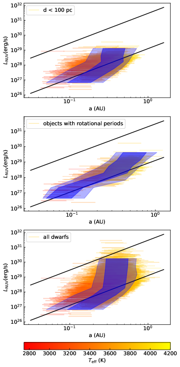
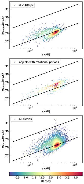
Figure 13: The relation between NUV luminosity and the distance between star and planet. The horizontal lines in Figure 13 show the CHZ. The samples from top panel to bottom panel are the dwarfs within 100 pc, the stars with rotational periods, and all dwarfs. The color bar represent the different effective temperature of stars. The dark blue shaded area is the conservative CHZ, and the light blue shaded area is the more optimistic CHZ. The samples in Figure 13 are as same as left, the color bar represent the density of stars. The black lines are the boundary of UHZ.

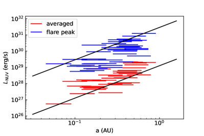
Figure 14: The relation between NUV luminosity and the star-planet distance of the sample with complete UV flares. The red lines are the normal luminosity of the stars, and the blue lines are the maximum luminosity of flare events.

6 UV observation by CSST

The China Space Station Telescope (CSST) is a space-borne optical-UV telescope, which is scheduled to be launched around 2024 (Ji et al., 2023). It is designed with a primary mirror with a diameter of 2 meters. CSST is equipped with seven photometric imaging bands and three spectroscopic bands, covering a wide range of wavelengths from the near-ultraviolet (NUV) to the near-infrared (NIR) (Zhan, 2011). CSST offers a large field of view (FOV) of approximately 1.1 deg² with a spatial resolution of $0.15^{"}$ for photometric imaging. In the NUV band, CSST covers a wavelength range from 252 to 321 nm, with a detection limit about 25 mag, much deeper than that of the GALEX telescope. In order to explore the potential of studies on UV activity using CSST, we obtained the CSST NUV activity index from the SDSS $u$-band and GALEX NUV indices.

First, We cross-matched our sample with the SDSS DR16 catalog using TOPCAT, and found 5,770 targets with SDSS $u$-band magnitudes. The activity index of the SDSS $u$ band was calculated with steps similar to $R^{\prime}_{\rm NUV}$, following

$$R^{\prime}_{\rm u}=\frac{f_{\rm u,exc}}{f_{\rm bol}}=\frac{f_{\rm u,obs}\times(\frac{d}{R})^{2}-f_{\rm u,ph}}{f_{\rm bol}}$$ (20)

The observed flux was estimated from $u$-band magnitude:

$$f_{\rm u}\ \rm{(erg\ s^{-1}\ cm^{-2})}=\rm 10^{-0.4\times(m_{u}+48.60-R_{u}\times E(B-V))}\times\delta\nu_{\rm u},$$ (21)

where $\delta\nu_{\rm u}$ represents the frequency range corresponding to the effective bandwidth of the $u$ band, which was calculated as the range of wavelengths ($\approx$807.34 Å) where the effective area falls to 10% of its peak. The $u$-band photospheric flux density was also derived using BT-Settl (AGSS2009) stellar spectral models.

Second, we obtained the CSST NUV activity index by interpolating between the SDSS $u$-band index and GALEX NUV index using their effective wavelengths (i.e., 2877 Å for CSST NUV band, 2316 Å for GALEX NUV band, and 3608 Å for SDSS $u$ band). Figure 15 shows the activity-rotation relation constructed from the CSST NUV band data. The results are more diffuse compared to the GALEX NUV band index, which may be caused by the interpolation.

Figure 16 shows the magnitude versus temperature diagram for the GALEX NUV band (left panel) and CSST NUV band (right panel). The diffuse distribution of GALEX NUV magnitudes suggests dominance by various chromospheric emissions, while the tight distribution of CSST NUV magnitudes indicates emissions dominated by the photosphere. In the temperature range of 3500–4000 K, the photospheric flux of the CSST NUV band accounts for about 60%–80% of the total flux. Accurate photometry and careful exclusion of the photospheric contribution are necessary for activity studies using the CSST NUV band. Whatever, it is promising to investigate UV activity of numerous M stars (as far as 10–15 kpc) through CSST observations, particularly for faint stars that are below the detection limit of current telescopes.

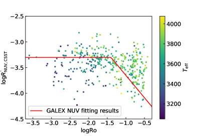
Figure 15: The activity-rotation relation of CSST NUV band. The red line is the fitting result from the GALEX NUV band.

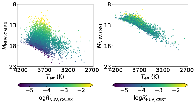
Figure 16: The magnitude vs. temperature diagram of GALEX NUV band (left panel) and CSST NUV band (right panel). The color bar of them are $R^{\prime}_{\rm NUV,GALEX}$ and $R^{\prime}_{\rm NUV,CSST}$, respectively.

7 Summary

By combining the LAMOST DR9 catalog and GALEX UV archive data, we studied chromospheric and UV activities of 6,629 M-type stars, including 5907 dwarfs, among which 582 ones have rotational period estimations, and 722 giants.

All the chromospheric and UV activity indices (i.e., $R^{\prime}_{\rm FUV}$, $R^{\prime}_{\rm NUV}$, $R^{\prime}_{\rm{HK}}$, and $R^{\prime}_{\rm{H\alpha}}$) clearly exhibit the saturated and unsaturated regions and the activity-rotation relation, in good agreement with previous studies. Most cooler stars tend to occupy in the saturated region, while hotter ones are located in the unsaturated regime. Both the FUV and NUV activity indices exhibit a wide single-peaked distribution. On the other hand, the H$\alpha$ and Ca II H$\&$K indices show a distinct double-peaked distribution. The gap between these peaks is most likely due to a rapid transition from a fast-rotating saturated population to a slow-rotating unsaturated one, suggesting a lack of stars with intermediate rotational periods and thus a discontinuous spin-down evolution. The clear difference in the rotational periods between the two populations further indicate that a rapid decay of the rotation period (during a stage of stellar evolution) leads to a significant weakening of stellar activity, especially for early-type M stars. On the other hand, for the late-type M stars, the multipole magnetic field exhibits weak magnetic breaking, leading to a much slower rotation decay. The smoothly varying distribution from M0 to M6 subtypes suggests a rotation-dependent dynamo for both early-type (partly convective) to late-type (fully convective) M stars. In addition, the distributions of three galactic orbital parameters, including $Jz$, $zmax$, and $e$, indicate the saturated population are generally younger than the unsaturated one.

We examined the relationships between different activity proxies. The FUV and NUV indices exhibit a tight relation described by ${\rm log}R^{\prime}_{\rm FUV}=(1.00\pm 0.02)\times{\rm log}R^{\prime}_{\rm NUV}-(0.37\pm 0.08)$. The comparisons between the different proxies, especially $R^{\prime}_{\rm{H\alpha}}$ and $R^{\prime}_{\rm{HK}}$, reveal two subpopulations characterized by saturated and unsaturated. A piecewise fitting between the $R^{\prime}_{\rm{H\alpha}}$ and $R^{\prime}_{\rm{HK}}$ is better than a linear fitting. The relations between $R^{\prime}_{\rm NUV}$ and chromospheric indices are positive but scattered. The scatter primarily arises from a group of $\approx$400 stars with oversaturated UV activity (log$R^{\prime}_{\rm NUV}>-$2.5) but unsaturated chromospheric activity. We considered several potential explanations for these stars, including the presence of a white dwarf companion, a companion with a similar stellar type, contamination from surrounding environment, chance alignment of extragalatic sources, over-estimated extinction, or the possibility of a very young stellar population. However, none of these explanations could totally account for the characteristics of these stars. Future UV spectral observations with the Space Telescope Imaging Spectrograph (STIS) or the Cosmic Origins Spectrograph (COS), both mounted on Hubble speace telescope, may help confirm whether there is a white dwarf companion (Parsons et al., 2016). If confirmed, this would represent a new method to detect white dwarfs in binaries lacking white dwarf features in the optical spectra—by selecting stars with abnormally high UV activity and normal chromospheric activity.

We searched for flare events in each GALEX exposure and identified 43 complete flare events of 35 stars. The durations of these flares vary from about 60 to 900 seconds; the peak luminosities range from $10^{28}$ to $10^{31}$ erg/s; the flare energy spans from $10^{30}$ to $10^{34}$ erg. All of these properties are similar to those of optical flares (e.g., Yang et al., 2017).

The habitability of planets orbiting M-type stars is affected by stellar activity, especially ultraviolet activity. We calculated the CHZs and UHZs of each star, in order to investigate the proportion of habitable stars falling within the overlapping region of these two habitable zones. We found 68% M stars in the total sample and 44%/42%/41% stars within 100/50/25 pc are potentially habitable. The variation of UV luminosity due to random flux fluctuation or UV flare has a limited influence on the stellar habitability.

Finally, we calculated the stellar activity of SDSS $u$ band, and then obtained the stellar activity of CSST NUV band using interpolation. The typical (although somewhat scattered) activity-rotation relation of CSST NUV band suggests the potential for conducting UV activity studies through CSST observations in the future, especially for faint stars that fall below the detection limit of current telescopes.

Appendix A LAMOST spectra of stars with super high UV emission

Appendix B Activities of giants

There are 722 giants in the total sample of 6629 stars. We considered a star as a giant if its surface gravity (log$g$) value is smaller than 3.5. The atmospheric parameters of M giants observed by LAMOST, especially log$g$ and [Fe/H], have a significant systematic offset with other surveys, such as APOGEE. Therefore, we conducted a cross-match with APOGEE DR17 to obtain atmospheric parameters for the common sources. For the remaining giants, we calculated the [Fe/H] using the correlation between the $W1-W2$ color index and metallicity (Li et al., 2016). We calculated the activity indices of giants using the same method for dwarfs (Table 2 and 3). Giants exhibit much lower activity level (the median of log$R^{\prime}_{\rm NUV}$ is about $-$5) compared to dwarfs (the median of log$R^{\prime}_{\rm NUV}$ is about $-$3.5).

References

- Astudillo-Defru et al. (2017) Astudillo-Defru, N., Delfosse, X., Bonfils, X., et al. 2017, A&A, 600, A13, doi: 10.1051/0004-6361/201527078
- Bai et al. (2018) Bai, Y., Liu, J., Wicker, J., et al. 2018, ApJS, 235, 16, doi: 10.3847/1538-4365/aaaab9
- Bailer-Jones et al. (2021) Bailer-Jones, C. A. L., Rybizki, J., Fouesneau, M., Demleitner, M., & Andrae, R. 2021, AJ, 161, 147, doi: 10.3847/1538-3881/abd806
- Bianchi et al. (2011) Bianchi, L., Efremova, B., Herald, J., et al. 2011, MNRAS, 411, 2770, doi: 10.1111/j.1365-2966.2010.17890.x
- Bianchi et al. (2017) Bianchi, L., Shiao, B., & Thilker, D. 2017, ApJS, 230, 24, doi: 10.3847/1538-4365/aa7053
- Binney (2012) Binney, J. 2012, MNRAS, 426, 1324, doi: 10.1111/j.1365-2966.2012.21757.x
- Bochanski et al. (2009) Bochanski, J. J., Hawley, S. L., Reid, I. N., et al. 2009, in American Institute of Physics Conference Series, Vol. 1094, 15th Cambridge Workshop on Cool Stars, Stellar Systems, and the Sun, ed. E. Stempels, 977–980, doi: 10.1063/1.3099284
- Boro Saikia et al. (2018) Boro Saikia, S., Marvin, C. J., Jeffers, S. V., et al. 2018, A&A, 616, A108, doi: 10.1051/0004-6361/201629518
- Boudreaux et al. (2022) Boudreaux, E. M., Newton, E. R., Mondrik, N., Charbonneau, D., & Irwin, J. 2022, ApJ, 929, 80, doi: 10.3847/1538-4357/ac5cbf
- Bovy (2015) Bovy, J. 2015, ApJS, 216, 29, doi: 10.1088/0067-0049/216/2/29
- Cardelli et al. (1989) Cardelli, J. A., Clayton, G. C., & Mathis, J. S. 1989, ApJ, 345, 245, doi: 10.1086/167900
- Chen et al. (2018) Chen, X., Wang, S., Deng, L., de Grijs, R., & Yang, M. 2018, ApJS, 237, 28, doi: 10.3847/1538-4365/aad32b
- Chen et al. (2020) Chen, X., Wang, S., Deng, L., et al. 2020, ApJS, 249, 18, doi: 10.3847/1538-4365/ab9cae
- Christy et al. (2022) Christy, C. T., Jayasinghe, T., Stanek, K. Z., et al. 2022, arXiv e-prints, arXiv:2205.02239. https://arxiv.org/abs/2205.02239
- Cui et al. (2012) Cui, X.-Q., Zhao, Y.-H., Chu, Y.-Q., et al. 2012, Research in Astronomy and Astrophysics, 12, 1197, doi: 10.1088/1674-4527/12/9/003
- Dálya et al. (2018) Dálya, G., Galgóczi, G., Dobos, L., et al. 2018, MNRAS, 479, 2374, doi: 10.1093/mnras/sty1703
- Dotter et al. (2008) Dotter, A., Chaboyer, B., Jevremović, D., et al. 2008, ApJS, 178, 89, doi: 10.1086/589654
- Douglas et al. (2014) Douglas, S. T., Agüeros, M. A., Covey, K. R., et al. 2014, ApJ, 795, 161, doi: 10.1088/0004-637X/795/2/161
- Drake et al. (2014) Drake, A. J., Graham, M. J., Djorgovski, S. G., et al. 2014, ApJS, 213, 9, doi: 10.1088/0067-0049/213/1/9
- Du et al. (2021) Du, B., Luo, A. L., Zhang, S., et al. 2021, Research in Astronomy and Astrophysics, 21, 202, doi: 10.1088/1674-4527/21/8/202
- Duncan et al. (1991) Duncan, D. K., Vaughan, A. H., Wilson, O. C., et al. 1991, ApJS, 76, 383, doi: 10.1086/191572
- El-Badry et al. (2021) El-Badry, K., Rix, H.-W., & Heintz, T. M. 2021, MNRAS, 506, 2269, doi: 10.1093/mnras/stab323
- Fetherolf et al. (2022) Fetherolf, T., Pepper, J., Simpson, E., et al. 2022, arXiv e-prints, arXiv:2208.11721, doi: 10.48550/arXiv.2208.11721
- Fetherolf et al. (2023) —. 2023, ApJS, 268, 4, doi: 10.3847/1538-4365/acdee5
- Findeisen et al. (2011) Findeisen, K., Hillenbrand, L., & Soderblom, D. 2011, AJ, 142, 23, doi: 10.1088/0004-6256/142/1/23
- Garraffo et al. (2015) Garraffo, C., Drake, J. J., & Cohen, O. 2015, ApJ, 813, 40, doi: 10.1088/0004-637X/813/1/40
- Gentile Fusillo et al. (2021) Gentile Fusillo, N. P., Tremblay, P. E., Cukanovaite, E., et al. 2021, MNRAS, 508, 3877, doi: 10.1093/mnras/stab2672
- Green et al. (2015) Green, G. M., Schlafly, E. F., Finkbeiner, D. P., et al. 2015, ApJ, 810, 25, doi: 10.1088/0004-637X/810/1/25
- Großschedl et al. (2018) Großschedl, J. E., Alves, J., Meingast, S., et al. 2018, A&A, 619, A106, doi: 10.1051/0004-6361/201833901
- Han et al. (2023) Han, H., Wang, S., Bai, Y., et al. 2023, ApJS, 264, 12, doi: 10.3847/1538-4365/ac9eac
- Hartman et al. (2011) Hartman, J. D., Bakos, G. Á., Noyes, R. W., et al. 2011, AJ, 141, 166, doi: 10.1088/0004-6256/141/5/166
- Howard et al. (2022) Howard, E. L., Davenport, J. R. A., & Covey, K. R. 2022, Research Notes of the American Astronomical Society, 6, 96, doi: 10.3847/2515-5172/ac6e42
- Husser et al. (2013) Husser, T. O., Wende-von Berg, S., Dreizler, S., et al. 2013, A&A, 553, A6, doi: 10.1051/0004-6361/201219058
- Irwin et al. (2011) Irwin, J., Berta, Z. K., Burke, C. J., et al. 2011, ApJ, 727, 56, doi: 10.1088/0004-637X/727/1/56
- Jackman et al. (2023) Jackman, J. A. G., Shkolnik, E. L., Million, C., et al. 2023, MNRAS, 519, 3564, doi: 10.1093/mnras/stac3135
- Jayasinghe et al. (2020) Jayasinghe, T., Kochanek, C. S., Stanek, K. Z., et al. 2020, VizieR Online Data Catalog, II/366
- Ji et al. (2023) Ji, X., Deng, L., Chen, Y., Li, C., & Liu, C. 2023, Research in Astronomy and Astrophysics, 23, 075009, doi: 10.1088/1674-4527/accdc4
- Jiménez-Esteban et al. (2018) Jiménez-Esteban, F. M., Torres, S., Rebassa-Mansergas, A., et al. 2018, MNRAS, 480, 4505, doi: 10.1093/mnras/sty2120
- Jones & West (2016) Jones, D. O., & West, A. A. 2016, ApJ, 817, 1, doi: 10.3847/0004-637X/817/1/1
- Karoff et al. (2016) Karoff, C., Knudsen, M. F., De Cat, P., et al. 2016, Nature Communications, 7, 11058, doi: 10.1038/ncomms11058
- Kasting et al. (1993) Kasting, J. F., Whitmire, D. P., & Reynolds, R. T. 1993, Icarus, 101, 108, doi: 10.1006/icar.1993.1010
- Kirk et al. (2016) Kirk, B., Conroy, K., Prša, A., et al. 2016, AJ, 151, 68, doi: 10.3847/0004-6256/151/3/68
- Kopparapu et al. (2014) Kopparapu, R. K., Ramirez, R. M., SchottelKotte, J., et al. 2014, ApJ, 787, L29, doi: 10.1088/2041-8205/787/2/L29
- Kopparapu et al. (2013) Kopparapu, R. K., Ramirez, R., Kasting, J. F., et al. 2013, ApJ, 765, 131, doi: 10.1088/0004-637X/765/2/131
- Kuhn et al. (2021) Kuhn, M. A., de Souza, R., Castro-Ginard, A., et al. 2021, in American Astronomical Society Meeting Abstracts, Vol. 53, American Astronomical Society Meeting Abstracts, 329.01
- Lehtinen et al. (2020) Lehtinen, J. J., Spada, F., Käpylä, M. J., Olspert, N., & Käpylä, P. J. 2020, Nature Astronomy, 4, 658, doi: 10.1038/s41550-020-1039-x
- Li et al. (2021) Li, C.-q., Shi, J.-r., Yan, H.-l., et al. 2021, ApJS, 256, 31, doi: 10.3847/1538-4365/ac22a8
- Li et al. (2016) Li, J., Smith, M. C., Zhong, J., et al. 2016, ApJ, 823, 59, doi: 10.3847/0004-637X/823/1/59
- Lightkurve Collaboration et al. (2018) Lightkurve Collaboration, Cardoso, J. V. d. M., Hedges, C., et al. 2018, Lightkurve: Kepler and TESS time series analysis in Python, Astrophysics Source Code Library. http://ascl.net/1812.013
- Lomb (1976) Lomb, N. R. 1976, Ap&SS, 39, 447, doi: 10.1007/BF00648343
- Lovis et al. (2011) Lovis, C., Dumusque, X., Santos, N. C., et al. 2011, arXiv e-prints, arXiv:1107.5325, doi: 10.48550/arXiv.1107.5325
- Loyd et al. (2018) Loyd, R. O. P., France, K., Youngblood, A., et al. 2018, ApJ, 867, 71, doi: 10.3847/1538-4357/aae2bd
- Magaudda et al. (2020) Magaudda, E., Stelzer, B., Covey, K. R., et al. 2020, A&A, 638, A20, doi: 10.1051/0004-6361/201937408
- Marton et al. (2016) Marton, G., Tóth, L. V., Paladini, R., et al. 2016, MNRAS, 458, 3479, doi: 10.1093/mnras/stw398
- Marton et al. (2019) Marton, G., Ábrahám, P., Szegedi-Elek, E., et al. 2019, MNRAS, 487, 2522, doi: 10.1093/mnras/stz1301
- Marton et al. (2023) Marton, G., Ábrahám, P., Rimoldini, L., et al. 2023, A&A, 674, A21, doi: 10.1051/0004-6361/202244101
- Matt et al. (2015) Matt, S. P., Brun, A. S., Baraffe, I., Bouvier, J., & Chabrier, G. 2015, ApJ, 799, L23, doi: 10.1088/2041-8205/799/2/L23
- Matt et al. (2012) Matt, S. P., MacGregor, K. B., Pinsonneault, M. H., & Greene, T. P. 2012, ApJ, 754, L26, doi: 10.1088/2041-8205/754/2/L26
- McQuillan et al. (2013) McQuillan, A., Aigrain, S., & Mazeh, T. 2013, MNRAS, 432, 1203, doi: 10.1093/mnras/stt536
- McQuillan et al. (2014) McQuillan, A., Mazeh, T., & Aigrain, S. 2014, ApJS, 211, 24, doi: 10.1088/0067-0049/211/2/24
- Million et al. (2016) Million, C., Fleming, S. W., Shiao, B., et al. 2016, ApJ, 833, 292, doi: 10.3847/1538-4357/833/2/292
- Morrissey et al. (2007) Morrissey, P., Conrow, T., Barlow, T. A., et al. 2007, ApJS, 173, 682, doi: 10.1086/520512
- Morton (2015) Morton, T. D. 2015, isochrones: Stellar model grid package. http://ascl.net/1503.010
- Newton et al. (2017) Newton, E. R., Irwin, J., Charbonneau, D., et al. 2017, ApJ, 834, 85, doi: 10.3847/1538-4357/834/1/85
- Newton et al. (2016) —. 2016, ApJ, 821, 93, doi: 10.3847/0004-637X/821/2/93
- Noyes et al. (1984) Noyes, R. W., Weiss, N. O., & Vaughan, A. H. 1984, ApJ, 287, 769, doi: 10.1086/162735
- Parker (1975) Parker, E. N. 1975, ApJ, 198, 205, doi: 10.1086/153593
- Parsons et al. (2016) Parsons, S. G., Rebassa-Mansergas, A., Schreiber, M. R., et al. 2016, MNRAS, 463, 2125, doi: 10.1093/mnras/stw2143
- Patel et al. (2015) Patel, B. H., Percivalle, C., Ritson, D. J., Duffy, C. D., & Sutherland, J. D. 2015, Nature Chemistry, 7, 301, doi: 10.1038/nchem.2202
- Prsa et al. (2022) Prsa, A., Kochoska, A., Conroy, K. E., et al. 2022, VizieR Online Data Catalog, J/ApJS/258/16
- Ranjan et al. (2017) Ranjan, S., Wordsworth, R., & Sasselov, D. D. 2017, ApJ, 843, 110, doi: 10.3847/1538-4357/aa773e
- Rebassa-Mansergas et al. (2021) Rebassa-Mansergas, A., Solano, E., Jiménez-Esteban, F. M., et al. 2021, MNRAS, 506, 5201, doi: 10.1093/mnras/stab2039
- Reid & Hawley (2000) Reid, I. N., & Hawley, S. L. 2000, New light on dark stars. Red dwarfs, low-mass stars, brown dwarfs.
- Reinhold & Hekker (2020) Reinhold, T., & Hekker, S. 2020, VizieR Online Data Catalog, J/A+A/635/A43
- Rekhi et al. (2023) Rekhi, P., Ben-Ami, S., Perdelwitz, V., & Shvartzvald, Y. 2023, arXiv e-prints, arXiv:2306.17045, doi: 10.48550/arXiv.2306.17045
- Ren et al. (2013) Ren, J., Luo, A., Li, Y., et al. 2013, AJ, 146, 82, doi: 10.1088/0004-6256/146/4/82
- Ren et al. (2018) Ren, J. J., Rebassa-Mansergas, A., Parsons, S. G., et al. 2018, MNRAS, 477, 4641, doi: 10.1093/mnras/sty805
- Ren et al. (2020) Ren, J. J., Raddi, R., Rebassa-Mansergas, A., et al. 2020, ApJ, 905, 38, doi: 10.3847/1538-4357/abc017
- Richey-Yowell et al. (2023) Richey-Yowell, T., Shkolnik, E. L., Schneider, A. C., et al. 2023, arXiv e-prints, arXiv:2305.06561, doi: 10.48550/arXiv.2305.06561
- Rimmer et al. (2018) Rimmer, P. B., Xu, J., Thompson, S. J., et al. 2018, Science Advances, 4, eaar3302, doi: 10.1126/sciadv.aar3302
- Rimoldini et al. (2023) Rimoldini, L., Holl, B., Gavras, P., et al. 2023, A&A, 674, A14, doi: 10.1051/0004-6361/202245591
- Ritson & Sutherland (2012) Ritson, D., & Sutherland, J. D. 2012, Nature Chemistry, 4, 895, doi: 10.1038/nchem.1467
- Sagan (1973) Sagan, C. 1973, Journal of Theoretical Biology, 39, 195, doi: 10.1016/0022-5193(73)90216-6
- Samus et al. (2009) Samus, N. N., Kazarovets, E. V., Durlevich, O. V., Kireeva, N. N., & Pastukhova, E. N. 2009, VizieR Online Data Catalog, B/gcvs
- Santos et al. (2019) Santos, A. R. G., García, R. A., Mathur, S., et al. 2019, ApJS, 244, 21, doi: 10.3847/1538-4365/ab3b56
- Santos et al. (2020) Santos, A. R. G., Garcia, R. A., Mathur, S., et al. 2020, VizieR Online Data Catalog, J/ApJS/244/21
- Sanz-Forcada et al. (2010) Sanz-Forcada, J., García-Álvarez, D., Velasco, A., et al. 2010, in Solar and Stellar Variability: Impact on Earth and Planets, ed. A. G. Kosovichev, A. H. Andrei, & J.-P. Rozelot, Vol. 264, 478–483, doi: 10.1017/S1743921309993152
- Scargle (1982) Scargle, J. D. 1982, ApJ, 263, 835, doi: 10.1086/160554
- Schlegel et al. (1998) Schlegel, D. J., Finkbeiner, D. P., & Davis, M. 1998, ApJ, 500, 525, doi: 10.1086/305772
- Schneider & Shkolnik (2018) Schneider, A. C., & Shkolnik, E. L. 2018, AJ, 155, 122, doi: 10.3847/1538-3881/aaaa24
- Shields et al. (2016) Shields, A. L., Ballard, S., & Johnson, J. A. 2016, Phys. Rep., 663, 1, doi: 10.1016/j.physrep.2016.10.003
- Shkolnik & Barman (2014) Shkolnik, E. L., & Barman, T. S. 2014, AJ, 148, 64, doi: 10.1088/0004-6256/148/4/64
- Shkolnik et al. (2011) Shkolnik, E. L., Liu, M. C., Reid, I. N., Dupuy, T., & Weinberger, A. J. 2011, ApJ, 727, 6, doi: 10.1088/0004-637X/727/1/6
- Soszyński et al. (2016) Soszyński, I., Pawlak, M., Pietrukowicz, P., et al. 2016, Acta Astron., 66, 405, doi: 10.48550/arXiv.1701.03105
- Spada et al. (2018) Spada, F., Demarque, P., Kim, Y. C., Boyajian, T. S., & Brewer, J. M. 2018, in Rediscovering Our Galaxy, ed. C. Chiappini, I. Minchev, E. Starkenburg, & M. Valentini, Vol. 334, 362–363, doi: 10.1017/S1743921317007347
- Spinelli et al. (2023) Spinelli, R., Borsa, F., Ghirlanda, G., Ghisellini, G., & Haardt, F. 2023, MNRAS, 522, 1411, doi: 10.1093/mnras/stad928
- Stelzer et al. (2016) Stelzer, B., Damasso, M., Scholz, A., & Matt, S. P. 2016, MNRAS, 463, 1844, doi: 10.1093/mnras/stw1936
- Stelzer et al. (2013) Stelzer, B., Marino, A., Micela, G., López-Santiago, J., & Liefke, C. 2013, MNRAS, 431, 2063, doi: 10.1093/mnras/stt225
- Toupance et al. (1977) Toupance, G., Bossard, A., & Raulin, F. 1977, Origins of Life, 8, 259, doi: 10.1007/BF00930687
- VanderPlas (2018) VanderPlas, J. T. 2018, ApJS, 236, 16, doi: 10.3847/1538-4365/aab766
- Vaughan & Preston (1980) Vaughan, A. H., & Preston, G. W. 1980, PASP, 92, 385, doi: 10.1086/130683
- Walkowicz et al. (2004) Walkowicz, L. M., Hawley, S. L., & West, A. A. 2004, PASP, 116, 1105, doi: 10.1086/426792
- Wang et al. (2020) Wang, S., Bai, Y., He, L., & Liu, J. 2020, ApJ, 902, 114, doi: 10.3847/1538-4357/abb66d
- Wang et al. (2022) Wang, Y.-F., Luo, A. L., Chen, W.-P., et al. 2022, A&A, 660, A38, doi: 10.1051/0004-6361/202142009
- Welsh et al. (2007) Welsh, B. Y., Wheatley, J. M., Seibert, M., et al. 2007, ApJS, 173, 673, doi: 10.1086/516640
- Wenger et al. (2000) Wenger, M., Ochsenbein, F., Egret, D., et al. 2000, A&AS, 143, 9, doi: 10.1051/aas:2000332
- West et al. (2015) West, A. A., Weisenburger, K. L., Irwin, J., et al. 2015, ApJ, 812, 3, doi: 10.1088/0004-637X/812/1/3
- Wright & Drake (2016) Wright, N. J., & Drake, J. J. 2016, Nature, 535, 526, doi: 10.1038/nature18638
- Yang & Liu (2019) Yang, H., & Liu, J. 2019, ApJS, 241, 29, doi: 10.3847/1538-4365/ab0d28
- Yang et al. (2017) Yang, H., Liu, J., Gao, Q., et al. 2017, ApJ, 849, 36, doi: 10.3847/1538-4357/aa8ea2
- Zhan (2011) Zhan, H. 2011, Scientia Sinica Physica, Mechanica & Astronomica, 41, 1441, doi: 10.1360/132011-961
- Zhang et al. (2022) Zhang, B., Jing, Y.-J., Yang, F., et al. 2022, ApJS, 258, 26, doi: 10.3847/1538-4365/ac42d1
- Zhong et al. (2019) Zhong, J., Li, J., Carlin, J. L., et al. 2019, ApJS, 244, 8, doi: 10.3847/1538-4365/ab3859
- Zong et al. (2020) Zong, W., Fu, J.-N., De Cat, P., et al. 2020, ApJS, 251, 15, doi: 10.3847/1538-4365/abbb2d