Abstract.

We consider a quasi-Bayesian method that combines a frequentist estimation in the first stage and a Bayesian estimation/inference approach in the second stage. The study is motivated by structural discrete choice models that use the control function methodology to correct for endogeneity bias. In this scenario, the first stage estimates the control function using some frequentist parametric or nonparametric approach. The structural equation in the second stage, associated with certain complicated likelihood functions, can be more conveniently dealt with using a Bayesian approach. This paper studies the asymptotic properties of the quasi-posterior distributions obtained from the second stage. We prove that the corresponding quasi-Bayesian credible set does not have the desired coverage in large samples. Nonetheless, the quasi-Bayesian point estimator remains consistent and is asymptotically equivalent to a frequentist two-stage estimator. We show that one can obtain valid inference by bootstrapping the quasi-posterior that takes into account the first-stage estimation uncertainty.

Key words: Bayesian methods, Bernstein–von Mises theorem, endogenous regressors, control function, semiparametric estimation
 

JEL classification: C11, C14, C15, C25

1. Introduction

The control function approach is commonly used in empirical economic studies to cope with endogenous explanatory variables in the structural equations (Heckman and Robb, 1985; Wooldridge, 2015). This approach typically involves two stages: the first stage projects the endogenous explanatory variables to a set of instruments and other exogenous variables and obtains the residuals; these residuals serve as control functions in the second stage as extra explanatory variables when estimating the structural equations. In this paper, we propose a quasi-Bayesian method that combines a frequentist-type first-stage estimation with some Bayesian approach in the second stage. The study is motivated by structural discrete choice models that apply the control function method to correct for endogeneity bias. In such scenarios, the second-stage estimation remains challenging for frequentist methods. The practical computational convenience of our proposal is easy to digest because the Bayesian paradigm turns the challenging integration or optimization problem in the second stage into a sampling problem of posterior distributions. Therefore, this quasi-Bayesian approach offers researchers great flexibility to combine various nonparametric frequentist methods with state-of-the-art Bayesian algorithms. With a clear understanding of its theoretical foundation, this new procedure can be particularly useful in econometric models with sophisticated likelihood and endogeneity issues.

To formalize the idea, we consider independent and identically distributed ($i.i.d.$) observations ${\bm{Y}}^{n}=(Y_{i},i=1,\cdots,n)^{\top}$. The component $\zeta_{0}$ represents a vector of unknown functions that one needs to estimate from the first-stage equation in order to obtain the residuals. Throughout the paper, we assume that the true $\zeta_{0}$ is identifiable and can be estimated from the subvector ${\bm{Y}}^{n}_{1}=(Y_{1,i},i=1,\cdots,n)^{\top}$ that consists of the observables from the first stage. We denote the resulting estimator by $\widehat{\zeta}_{n}$. The second stage postulates a probability density function, $p_{\theta}^{n}(\cdot;\zeta)$ for the subvector ${\bm{Y}}^{n}_{2}=(Y_{2,i},i=1,\cdots,n)^{\top}$ determined by the structural equation with the unknown parameter of interest $\theta\in\Theta\subset\mathbb{R}^{p}$, for some integer $p\geq 1$. The unique truth is denoted by $\theta_{0}$. The Bayesian approach in the second stage posits a prior distribution $\Pi(\theta)$ and updates this prior to the quasi-posterior distribution given the limited-information likelihood in the second stage. Using the Bayes’ rule, the quasi-posterior of the finite-dimensional parameter $\theta$ is

(1.1) $$\Pi[\theta\in\mathcal{A}|{\bm{Y}}_{2}^{n};\widehat{\zeta}_{n}]=\frac{\int_{\mathcal{A}}p^{n}_{\theta}({\bm{Y}}_{2}^{n};\widehat{\zeta}_{n})d\Pi(\theta)}{\int_{\Theta}p^{n}_{\theta^{\prime}}({\bm{Y}}_{2}^{n};\widehat{\zeta}_{n})d\Pi(\theta^{\prime})}.$$

We refer to the estimation/inferential procedure derived from the above posterior as quasi-Bayesian because the term $p^{n}_{\theta}({\bm{Y}}_{2}^{n};\widehat{\zeta}_{n})$ is not a genuine likelihood, and it depends on some plug-in estimator $\widehat{\zeta}_{n}$. Two key questions arise: (1). Is the quasi-posterior distribution of $\theta$ asymptotically Gaussian? (2). What are the center and dispersion of this quasi-posterior distribution? To our best knowledge, such problems have not been investigated in the literature even when the estimator $\widehat{\zeta}_{n}$ is entirely parametric. Our paper fills this void, and we allow for any flexible first-stage nonparametric estimation.

Our main objective is to provide a thorough theoretical understanding of the large sample properties of this quasi-Bayesian procedure from the frequentist’s perspective. The challenge is that one faces a nonstandard posterior distribution that depends on the first-stage estimation. It is unclear whether the corresponding quasi-Bayesian credible set agrees with the frequentist’s confidence set, even asymptotically. We show that this credible set does not have the right coverage in large samples because it ignores the estimation uncertainty from the first stage. On the other hand, the quasi-Bayesian point estimator, such as the quasi-posterior mean, is asymptotically equivalent to a frequentist two-stage estimator; that is, it is root-$n$ asymptotically normal with the same sandwich-type covariance matrix as its frequentist counterpart. In essence, the quasi-posterior distribution is correctly centered but with a wrong dispersion. We also show that a proper bootstrap method will restore the desirable coverage probability and thus is valid for inference. Although the bootstrap requires additional simulation, its implementation can be easily parallelized.

To illustrate our theory, we focus on an endogenous multinomial Probit (MNP) model from Petrin and Train (2010), which we refer to as the Petrin–Train model in the sequel. The framework is popular in modeling consumer choices over different products, say choosing from $j\in\{0,\cdots,J\}$, with the $0$-th category being the non-purchase option. The endogenous variable $(X_{j}^{e})_{j=0}^{J}$ can be the price, advertising, or quality in the context. To address the endogeneity problem, researchers often construct the Hausman-type price instruments (Petrin and Train, 2010). The first stage involves the estimation of a vector of $(\zeta_{j})_{j=0}^{J}$, as the conditional mean functions of the endogenous variables given the exogenous covariates and instrument variables. Given the estimated conditional mean functions $\widehat{\zeta}_{n}=(\widehat{\zeta}_{n,j})_{j=0}^{J}$, we can extract the residuals as the control functions or variables for the second-stage MNP model. In this scenario, the likelihood function $p^{n}_{\theta}({\bm{Y}}_{2}^{n};\widehat{\zeta}_{n})$ is the product of the conditional choice probabilities that involve complicated multiple integrals. As reviewed in Train (2009), the Bayesian approach enjoys practical advantages over frequentist methods in estimating the MNP-type models.

Going beyond the Petrin-Train model, our study reflects two generic features of modern econometric models. On the one hand, many models used to describe observed data may be so complex that the likelihoods associated with these models are computationally intractable. These analytical difficulties can be alleviated by simulation-based procedures, such as the Bayesian method, which has proven successful in many areas. On the other hand, the control function approach provides an effective solution to deal with the endogeneity problem. This approach treats endogeneity as an omitted variable bias problem, in which the inclusion of estimates of the first-stage errors as additional covariates corrects the inconsistency of the second stage. The idea of combining a frequentist first stage and a Bayesian second stage has been practiced in empirical research (Agarwal and Somaini, 2018), though lacking a formal theoretical investigation for such a “hybrid” or quasi-Bayesian procedure. In their empirical analysis of the distribution of students’ preferences for public schools, Agarwal and Somaini (2018) first estimate the believed assignment probabilities at various schools using frequentist methods and then conduct Bayesian estimation in the second stage due to a complicated likelihood similar to the MNP. They also suggest a bootstrap method for inference. Our paper sheds a theoretical light on the asymptotic normality of the two-stage quasi-Bayesian estimator and the bootstrap validity therein.

There is a clear advantage of our proposal over the frequentist two-step method or the Bayesian full information paradigm in the current context, because it separates two tasks: one can correct for the endogeneity bias via robust nonparametric first-stage estimation, while tackling the complicated likelihood in the second stage by a Bayesian approach. This separation of tasks allows for considerable algorithmic flexibility. Regarding the frequentist two-step approach, the second stage requires the simulated method of moments (McFadden, 1989; Hajivassiliou and McFadden, 1998), which calls for Monte Carlo simulation, in addition to solving hard optimization problems for finding the frequentist type point estimator. Referring to the full information Bayesian approach, one would focus on the posterior that is proportional to $\tilde{p}^{n}_{\theta,\zeta}({\bm{Y}}^{n})d\Pi(\theta)dQ(\zeta)$, where $\tilde{p}^{n}_{\theta,\zeta}({\bm{Y}}^{n})$ is the density function for the joint distribution of $\bm{Y}^{n}_{1}$ and $\bm{Y}^{n}_{2}$ combining two stages together, and $Q(\cdot)$ is a suitable prior on the functional component $\zeta$. The joint likelihood inevitably requires a full model encompassing both stages, for which the applied researcher may be reluctant to hypothesize such a structure (Murphy and Topel, 2002). If the researcher does not want to assume a parametric model for $\zeta$, the full-information Bayes must put a nonparametric prior $Q(\zeta)$ on it. Although the non-parametric Bayesian inference is one of the most vibrant research areas in econometric theory, verification of the related Bernstein–von Mises (BvM) theorem either relies on the Gaussian processes priors or explores particular model structures; see Ghosal and van der Vaart (2017). In addition, designing a feasible algorithm for the posteriors remains a skillful task when the joint likelihood functions from both stages are combined.

1.1. Related Literature

Studying asymptotic properties of quasi-Bayesian procedures forms an important line of work in econometrics. Regarding the discrepancy between quasi-Bayesian credible sets and frequentist confidence sets, we highlight a recurring theme when the generalized information identity fails (Chernozhukov and Hong, 2003). In this case, the local asymptotic normality (LAN) expansion (van der Vaart, 1998) generates a centering term whose asymptotic variance is of the sandwich form that does not match the (minus) second derivative matrix of the (quasi) log-likelihood function. These phenomena appear in studies of the generalized method of moments (GMM) or the limited information approach (Kim, 2002; Chernozhukov and Hong, 2003; Chib, Shin, and Simoni, 2018), as well as in misspecified models (Kleijn and van der Vaart, 2012; Müller, 2013; Kim, 2014). Given the natural link between GMM and two-step estimation (Newey and McFadden, 1994), it is tempting to think that our framework is nested by the works mentioned above. This is not the case. We emphasize that one distinct feature of our problem is that the first-stage estimation is based on a frequentist method and then plugged into the posterior of the second stage. One can view this as approximating the posterior of $\zeta$ using an infinitely narrow but tall spike at a given value, like the Dirac delta function. Such feature usually violates the standard assumptions in proving the BvM theorem.

Another line of research closely related to this paper is the profile sampler (Lee, Kosorok, and Fine, 2005; Cheng and Kosorok, 2008). This literature recommends sampling from the profile likelihood $pl_{n}(\theta)\equiv\sup_{\zeta}p^{n}_{\theta}({\bm{Y}}^{n};\zeta)$ for semiparametric models indexed by $(\theta,\zeta)$. The infinite-dimensional parameter $\zeta$ therein must be estimated via the profile maximum likelihood so that there is no additional adjustment term; also, see the last paragraph on page 1357 of Newey (1994) about the profiled out nuisance functions. Such procedures are not required in our setup. The crux of our analysis is to characterize the first-stage estimation effect on the quasi-Bayesian posteriors. On the technical ground, this paper also refines the proof of Lee, Kosorok, and Fine (2005) and Cheng and Kosorok (2008): we show the asymptotic negligibility of the posterior outside a shrinking neighborhood of the truth, where the radius depends on the convergence rate of first-stage estimation. In comparison, the result of Lemma A.1 of Lee, Kosorok, and Fine (2005) is stated for some neighborhood with a fixed radius, yet later on, this lemma is cited to cover the case with a shrinking radius of the order $o(n^{-1/3})$. Our proof relaxes this rate to match the well-known requirement at the order of $o(n^{-1/4})$ in general semiparametric models (Newey, 1994).

1.2. Organization

The rest of our paper is organized as follows: Section 2 contains the main theoretical results. This relatively long section is divided into three subsections, in which we introduce necessary assumptions, investigate the asymptotic behavior of the quasi-posterior for the finite-dimensional parameter in the second stage, and show the validity of bootstrap methods for inference. Section 3 applies the general theory to the Petrin–Train model. We present low-level regularity conditions and state the asymptotic results. Section 4 conducts Monte Carlo simulations and provides an empirical illustration. The last section concludes. Proofs of the main results are presented in Appendix A. More technical lemmas and their proofs are collected in Appendix B.

2. Main Theoretical Results

Bayesian methodology is attractive in its own right. Nonetheless, our problem is fundamentally non-Bayesian, as researchers aim to estimate unknown fixed parameters using the control function approach to correct the endogeneity bias. This motivates us to investigate the large sample behavior of the resulting quasi-posteriors under a fixed true probability model $P_{0}=P_{\theta_{0},\zeta_{0}}$ that generates the observed data. A thorough understanding will provide solid justification for the quasi-Bayesian methods, which can be attractive to non-Bayesian practitioners who use them because of their convenience.

We establish the asymptotic theory, drawing on two themes. The first is the frequentist two-step estimation and inference in econometrics literature (Newey, 1994; Chen, Linton, and Van Keilegom, 2003; Ichimura and Lee, 2010). The crux therein is how to characterize the influence of the first-step nonparametric estimation on the remaining parametric components and how to make proper adjustments for inference. This analysis is also central to our study, and we formally show how the quasi-posterior ignores the effect from the first-stage estimation. The second theme is the asymptotic analysis of Bayesian methods for semiparametric models. Our theoretical findings have not been reported before; they shed new light on the BvM theorem (van der Vaart, 1998; Ghosal and van der Vaart, 2017). For standard semiparametric models using full information Bayesian methods, the BvM theorem states that the marginal posterior for the finite-dimensional parameter is approximately a normal distribution centered at the semiparametric efficient estimator. Hence, the point estimators and credible sets are produced by one stroke therein. However, estimation and inference have to be dealt with separately for the quasi-posterior distribution in our setting.

2.1. Assumptions and Discussions

The (limited-information) log-likelihood function is of fundamental importance in the second-stage Bayesian estimation. Throughout the paper, we focus on the case with i.i.d. data, so the likelihood function becomes $p_{\theta}^{n}(\bm{Y}_{2}^{n};\zeta)=\prod_{i=1}^{n}p_{\theta}(Y_{2,i};\zeta)$ and the log-likelihood is denoted by $\ell_{n}(\theta;\zeta)\equiv\log p_{\theta}^{n}(\bm{Y}_{2}^{n};\zeta)=\sum_{i=1}^{n}\log p_{\theta}(Y_{2,i};\zeta)$. We define the following first-order derivative with respect to (w.r.t.) the finite-dimensional parameter $\theta$:

(2.1) $$\dot{l}_{\theta}\left(Y_{2},\theta;\zeta\right)\equiv\left(\frac{\partial\log p(Y_{2},\theta;\zeta)}{\partial\beta^{\top}},\frac{\partial\log p(Y_{2},\theta;\zeta)}{\partial\eta^{\top}}\right)^{\top},$$

where $\theta$ is partitioned into the parameter of interest $\beta$ and the nuisance parameter $\eta$. The metric associated with the parameter $\theta$ is $d_{\Theta}(\cdot,\cdot)$. The second-order derivative is denoted by $\ddot{l}_{\theta}\left(Y_{2},\theta;\zeta\right)$ in the same vein. Thereafter, the score function is $S_{\theta}\left(\theta,\zeta\right)=P_{0}\dot{l}_{\theta}\left(Y_{2},\theta;\zeta\right)$, with the corresponding empirical version as $S_{\theta,n}\left(\theta,\zeta\right)=\mathbb{P}_{n}\dot{l}_{\theta}\left(Y_{2},\theta;\zeta\right)$. The negative Hessian matrix $V_{0}=-P_{0}\ddot{l}_{\theta}\left(Y_{2},\theta_{0};\zeta_{0}\right)$ is the information matrix for the second-stage likelihood, when $\zeta_{0}$ is known. The unknown function in the first stage may contain multiple components, so we write $\zeta_{0}=(\zeta_{0j})_{j=0}^{J}$. Consider a map defined by $\Psi(\theta,\zeta)\equiv S_{\theta}(\theta,\zeta)$. The following pathwise derivative of $\Psi$ plays a key role in determining the effect of the first-stage estimation (Newey, 1994):

$$\dot{\Psi}_{\zeta}(\theta_{0},\zeta_{0})[\zeta-\zeta_{0}]:=\sum_{j=0}^{J}\dot{\Psi}_{\zeta_{j}}(\theta_{0},\zeta_{0})[\zeta_{j}-\zeta_{0j}],$$

where each $\dot{\Psi}_{\zeta_{j}}$ is a bounded linear functional that maps $\zeta_{j}-\zeta_{0j}$ to a real number. The proper functional space for $\zeta$ is denoted by $\mathcal{G}$ with its pseudo metric $d_{G}(\cdot,\cdot)$.

We list all regularity conditions followed by some heuristic discussions in order. They are not necessarily the weakest possible assumptions. For a function $f(\cdot)$ of a random vector $Y$ that follows distribution $P$, we use the standard empirical process notations: $P_{0}f=\int f(y)dP_{0}(y),\mathbb{P}_{n}f=n^{-1}\sum_{i=1}^{n}f(Y_{i})$, and $\mathbb{G}_{n}f=n^{1/2}\left(\mathbb{P}_{n}-P_{0}\right)f$. We also write $\mathbb{E}_{0}$ instead of $P_{0}$ in bounding center stochastic terms. Definitions of the $P_{0}$-Glivenko-Cantelli class and the $P_{0}$-Donsker class follow those in van der Vaart and Wellner (1996) and van der Vaart (1998).

Assumption 2.1 (Identification).

The function $\zeta_{0}$ is uniquely identified from the first stage. The expected log-likelihood function $\mathbb{E}_{0}[\log p_{\theta}(Y_{2};\zeta_{0})]$ has a unique maximum at $\theta_{0}$ over the parameter space $\Theta$ in the sense that $\sup_{d_{\Theta}(\theta,\theta_{0})>\delta}\mathbb{E}_{0}[\log p_{\theta}(Y_{2};\zeta_{0})]<\mathbb{E}_{0}[\log p_{\theta_{0}}(Y_{2};\zeta_{0})]$ for any $\delta>0$. Also, $S_{\theta}\left(\theta_{0},\zeta_{0}\right)=0$, and the matrix $V_{0}$ is positive definite with its smallest eigenvalue $\lambda_{1}>0$.

Assumption 2.2 (First-stage Estimation).

The first-stage estimator $\widehat{\zeta}_{n}\in\mathcal{G}_{n}$ with probability 1, and $d_{G}(\widehat{\zeta}_{n},\zeta_{0})=O_{P_{0}}(r_{n})$, where $r_{n}=o(n^{-1/4})$ and $nr_{n}^{2}\to+\infty$.

Assumption 2.3 (Frequentist Two-stage Estimation).

There exists a frequentist-type estimator that approximately maximizes the second-stage likelihood, i.e., $\widehat{\theta}_{n}=\arg\max_{\theta}\ell_{n}(\theta;\widehat{\zeta}_{n})+o_{P_{0}}(n^{-1/2})$. In addition, it satisfies

(2.2) $$S_{\theta,n}\left(\widehat{\theta}_{n},\widehat{\zeta}_{n}\right)=o_{P_{0}}(n^{-1/2}).$$

Assumption 2.4 (Prior).

The prior measure $\Pi$ on $\Theta$ is assumed to be a probability measure with a bounded Lebesgue density $\pi$, which is continuous and positive on a neighborhood of the true value $\theta_{0}$. In addition, $\int|\theta|^{a}\pi(\theta)d\theta<+\infty$, for $a\geq 0$.

Assumption 2.5 (Smoothness).

We assume the log-likelihood function satisfies the following restrictions for some positive constant terms $C_{1},\cdots,C_{4}$:

$$\sup_{\zeta\in\mathcal{G}_{n}}\left|\mathbb{E}_{0}\left[\log p_{\theta_{0}}(\cdot;\zeta)-\log p_{\theta_{0}}(\cdot;\zeta_{0})\right]\right|\leq C_{1}r_{n}^{2},$$

and

$$\mathbb{E}_{0}\left[\log p_{\theta}(\cdot;\zeta)-\log p_{\theta_{0}}(\cdot;\zeta_{0})\right]+e_{n}(\theta,\zeta)\leq-C_{2}d^{2}_{\Theta}(\theta,\theta_{0})+C_{3}d^{2}_{G}(\zeta,\zeta_{0}),$$

for some $e_{n}(\cdot,\cdot)$ that satisfies

$$\sup_{d_{\Theta}(\theta,\theta_{0})\leq\rho,\zeta\in\mathcal{G}_{n}}|e_{n}(\theta,\zeta)|\leq C_{4}\rho r_{n}.$$

Assumption 2.6 (Differentiability).

The function $\mathbb{E}_{0}[\log p_{\theta}(Y_{2i};\zeta)]$ is continuous with respect to $\zeta$ uniformly in $\theta\in\Theta$. The function $\Psi(\theta,\zeta)$ is Fréchet differentiable at $(\theta_{0},\zeta_{0})$, i.e. there exists a continuous and non-singular matrix $\dot{\Psi}_{\theta}(\theta_{0},\zeta_{0})$ and a continuous linear functional $\dot{\Psi}_{\zeta}(\theta_{0},\zeta_{0})$ such that

$$\parallel\Psi(\theta,\zeta)-\Psi(\theta_{0},\zeta_{0})-\dot{\Psi}_{\theta}(\theta_{0},\zeta_{0})(\theta-\theta_{0})-\dot{\Psi}_{\zeta}(\theta_{0},\zeta_{0})[\zeta-\zeta_{0}]\parallel\leq o(d_{\Theta}(\theta,\theta_{0}))+O(d^{2}_{G}(\zeta,\zeta_{0})).$$

Assumption 2.7 (Complexity).

(i) The functional classes $\{\log p_{\theta}(Y_{2i};\zeta):\theta\in\Theta,\zeta\in\mathcal{G}_{n}\}$ and $\left\{\ddot{l}_{\theta}(\cdot,\theta;\zeta):\theta\in\Theta,\zeta\in\mathcal{G}_{n}\right\}$ belong to $P_{0}$-Glivenko-Cantelli classes. (ii) The functional class $\{\dot{l}_{\theta}(Y_{2},\theta_{0};\zeta):\zeta\in\mathcal{G}_{n}\}$ belongs to a $P_{0}$-Donsker class. The following functional class

$$\{\log p_{\theta}(Y_{2};\zeta)-\log p_{\theta_{0}}(Y_{2};\zeta)-(\theta-\theta_{0})^{\top}\dot{l}_{\theta_{0}}(;\zeta):d_{\Theta}(\theta,\theta_{0})\leq Cr_{n},\zeta\in\mathcal{G}_{n}\}$$

divided by each ordinates of $(\theta-\theta_{0})$ belongs to a $P_{0}$-Donsker class with its second moment going to zero w.p.1. (iii) There exists some function $\phi_{n}(\cdot)$ such that

$$\mathbb{E}_{0}\left[\sup_{d_{\Theta}(\theta,\theta_{0})\leq\rho,\zeta\in\mathcal{G}_{n}}\mathbb{G}_{n}\left|\log p_{\theta}(\cdot,\theta;\zeta)-\log p_{\theta}(\cdot,\theta_{0};\zeta)\right|\right]\leq\phi_{n}(\rho),$$

for $\rho\geq r_{n}$. $\phi_{n}(\cdot)$ is a sequence of functions defined on $(0,\infty)$ that satisfies: $\rho\mapsto\phi_{n}(\rho)/\rho^{\gamma}$ is decreasing for some $\gamma<2$; $\rho^{-2}\phi_{n}(\rho)\leq\sqrt{n}$ for every $n$.

Assumption 2.8 (Normality).

Let $\Delta_{n,0}\equiv\sqrt{n}\left(S_{\theta,n}(\theta_{0},\zeta_{0})+\dot{\Psi}_{\zeta}(\theta_{0},\zeta_{0})[\widehat{\zeta}_{n}-\zeta_{0}]\right)$. Assume that the following linear representation holds:

$$\Delta_{n,0}=\frac{1}{\sqrt{n}}\sum_{i=1}^{n}\left[\Gamma_{2}(Y_{2i})+\Gamma_{1}(Y_{1i})\right]+o_{P_{0}}(1),$$

with the influence function $\Gamma_{2}(\cdot)+\Gamma_{1}(\cdot)$. Also, the following asymptotic normality holds:

$$\frac{1}{\sqrt{n}}\sum_{i=1}^{n}\left[\Gamma_{2}(Y_{2i})+\Gamma_{1}(Y_{1i})\right]\Rightarrow\mathbb{N}(0,\Omega_{0}),$$

for some finite covariance matrix $\Omega_{0}$.

Assumptions 2.1 to 2.3 are generic, concerning the identifiability of the model parameters, the asymptotics of the first stage nonparametric estimation, as well as the existence of a frequentist two-stage estimator. The frequentist two-stage estimator $\widehat{\theta}_{n}$ merely serves as a theoretical device, as it will become the centering point in the local asymptotic normal (LAN) expansion (Ghosh and Ramamoorthi, 2002; Chernozhukov and Hong, 2003; Lee, Kosorok, and Fine, 2005). In our context of analyzing structural discrete choice models, $\widehat{\theta}_{n}$ is difficult to compute, which motivates the quasi-Bayesian procedure. The Assumption 2.4 on the prior density is also standard (Ghosh and Ramamoorthi, 2002; Chernozhukov and Hong, 2003).

Compared with the standard conditions for the BvM theorem (van der Vaart, 1998), our setting involves two complications due to the presence of the estimated control function. The first task is to ensure that the posterior probability concentrates in any small neighborhood of the true parameter uniformly over a set $\mathcal{G}_{n}$ to which the estimated $\widehat{\zeta}_{n}$ belongs. The second distinction is that one needs an adjustment term in the LAN expansion, which accounts for the first-stage estimation error. Assumptions 2.5 and 2.7 (iii) are needed to ensure that the quasi-likelihood ratio decays exponentially fast for $\{\theta:d_{\Theta}(\theta,\theta_{0})>\delta\}$ with a fixed radius $\delta>0$, as well as to strengthen the exponential type decay for $\{\theta:Cr_{n}\leq d_{\Theta}(\theta,\theta_{0})\leq\delta\}$, with the rate $r_{n}$ stated in Assumption 2.2. The differentiability condition in Assumption 2.6 w.r.t. $\theta$ and $\zeta$ are needed to account for the two stages in our quasi-Bayesian method. Finally, Assumption 2.8 is used in the LAN expansion of the log-likelihood ratio.

2.2. Large Sample Behaviors of Quasi-Posteriors

Our main use of the quasi-posterior is to interpret it as a frequentist’s device, similar to that of a sampling distribution. Also, we are interested in whether the mean of this quasi-posterior is a legitimate point estimator for $\theta_{0}$. Define the posterior density function of $h\equiv\sqrt{n}(\theta-\widehat{\theta}_{n})$ by

$$\tilde{\pi}(h|\bm{Y}_{2}^{n};\widehat{\zeta}_{n})\equiv\frac{p^{n}_{\widehat{\theta}_{n}+\frac{h}{\sqrt{n}}}(\bm{Y}_{2}^{n}|\widehat{\zeta}_{n})\pi(\widehat{\theta}_{n}+\frac{h}{\sqrt{n}})}{\int p^{n}_{\widehat{\theta}_{n}+\frac{h}{\sqrt{n}}}(\bm{Y}_{2}^{n}|\widehat{\zeta}_{n})\pi(\widehat{\theta}_{n}+\frac{h}{\sqrt{n}})dh}.$$

Furthermore, the limiting normal density is

$$\pi_{\infty}(h)\equiv(2\pi)^{-p/2}|\det V_{0}|^{1/2}\exp\left\{-\frac{h^{\top}V_{0}h}{2}\right\}.$$

In order to metrize the weak convergence, we consider the following “total variation of moments” norm (Chernozhukov and Hong, 2003) for a real-valued function $f$ on $\mathcal{S}$ as

$$\|f\|_{TVM(a)}\equiv\int_{\mathcal{S}}(1+|h|^{a})|f(h)|dh,$$

for some $a\geq 0$.

Theorem 2.1 (Posterior Measures).

Suppose Assumptions 2.1 to 2.8 hold. Then, we have

(2.3) $$\|\tilde{\pi}(h|\bm{Y}_{2}^{n};\widehat{\zeta}_{n})-\pi_{\infty}(h)\|_{TVM(a)}=o_{P_{0}}(1).$$

Consequently, the rescaled sequence of quasi-posteriors for $\theta$ converges in total variation to a standard normal measure, that is,

(2.4) $$\sup_{\xi\in\mathbb{R}^{p}}|\Pi(\sqrt{n}V_{0}^{1/2}(\theta-\widehat{\theta}_{n})\leq\xi|{\bm{Y}}^{n}_{2};\widehat{\zeta}_{n})-\Phi_{p}(\xi)|\to_{P_{0}}0.$$

where $\Phi_{p}(\cdot)$ denotes the $p$-dimensional standard normal distribution.

Let $\mathcal{C}_{n}(\alpha)$ be the quasi-Bayesian credible set constructed from the quasi-posterior, that is, $\mathcal{C}_{n}(\alpha)$ satisfies $\Pi(\theta\in\mathcal{C}_{n}(\alpha)|{\bm{Y}}^{n}_{2};\widehat{\zeta}_{n})=1-\alpha$ for a given nominal level $\alpha\in(0,1)$. An important implication of Theorem 2.1 is that $\mathcal{C}_{n}(\alpha)$ does not have the correct asymptotic coverage probability in general, as stated in Corollary 2.1.

Corollary 2.1.

Let $B_{n}$ be the set that satisfies $(2\pi)^{-p/2}\int_{B_{n}}e^{-h^{\top}h/2}dh\to 1-\alpha$ as $n\to\infty$, and recall the definition of $\Delta_{n,0}$ in Assumption 2.8. Under the same assumptions for Theorem 2.1, we have

(2.5) $$P_{0}\{\theta_{0}\in\mathcal{C}_{n}(\alpha)\}=P_{0}\{-V_{0}^{-1/2}\Delta_{n,0}\in B_{n}\}.$$

In addition, if $V_{0}=\Omega_{0}$, then we have

(2.6) $$P_{0}\{\theta_{0}\in\mathcal{C}_{n}(\alpha)\}\to 1-\alpha.$$

Theorem 2.1 may look similar to the standard parametric BvM theorem at first glance. However, the departures are the presence of the first-stage estimation $\widehat{\zeta}_{n}$ and the centering point $\widehat{\theta}_{n}$, which is a two-stage frequentist estimator whose asymptotic covariance matrix takes the sandwich form $V_{0}^{-1}\Omega_{0}V_{0}^{-1}$, where $\Omega_{0}$ corresponds to the variance of $\Gamma_{2}(Y_{2i})+\Gamma_{1}(Y_{1i})$ in Assumption 2.8. On the other hand, as Corollary 2.2 below shows, the variance of the quasi-posterior of $\theta$ is governed by the information matrix $V_{0}$, which only captures the variance of $\Gamma_{2}(Y_{2i})$. The discrepancy between $\Omega_{0}$ and $V_{0}$ prevents the right hand side of (2.5) from converging to the desired coverage probability $1-\alpha$ in general. With the additional restriction $V_{0}=\Omega_{0}$, which corresponds to the case where the generalized information equality holds (Chernozhukov and Hong, 2003), $\mathcal{C}_{n}(\alpha)$ will have the correct coverage probability coincidentally, as (2.6) shows. The general coverage failure of the quasi-Bayesian credible set is similar to what Kleijn and van der Vaart (2012) found when they studied the Bayesian procedure for misspecified models. Considering the formal decision theory of the interval estimation problem, Müller (2013) showed that the asymptotic risk of a vanilla posterior is worse than that of a modified posterior using the sandwich covariance matrix; see Section 2.4 of Müller (2013). Below, we show that the quasi-posterior mean is asymptotically equivalent to the frequentist’s two-stage estimator $\widehat{\theta}_{n}$. However, the rescaled posterior variance is not the same as the asymptotic variance of the frequentist two-stage estimator.

Corollary 2.2.

Denote the mean and variance of the quasi-posterior by $\widetilde{\theta}_{n}$ and $\widetilde{\mathrm{Var}}_{n}(\theta)$. Assume that the prior for $\theta$ satisfies $\int|\theta|^{2}d\Pi(\theta)<+\infty$. Then we have

(2.7) $$\widetilde{\theta}_{n}=\widehat{\theta}_{n}+o_{P_{0}}(n^{-1/2}),~{}\text{and}~{}n^{-1}\widetilde{\mathrm{Var}}_{n}(\theta)^{-1}=V^{-1}_{0}+o_{P_{0}}(1).$$

As a consequence of the first equality in (2.7), the quasi-posterior mean is asymptotically normal:

$$\sqrt{n}(\widetilde{\theta}_{n}-\theta_{0})\Rightarrow\mathbb{N}(0,V^{-1}_{0}\Omega_{0}V^{-1}_{0}).$$

Remark 2.1.

In the context of GMM, Chernozhukov and Hong (2003) constructed a quasi-likelihood by exponentiating the quadratic criterion function. Chernozhukov and Hong (2003) demonstrated that the weighting matrix can be properly chosen so that the generalized information identity holds, and the resulting posterior distribution can be utilized for asymptotically valid confidence sets. When the generalized information equality fails, Chernozhukov and Hong (2003) also suggested that the posterior still contains useful information for inference, as the posterior variance is related to the Hessian matrix. If $\Omega_{0}$ is easier to obtain, one can form the normal confidence interval by plugging in the sandwich-type covariance matrix estimator, which combines the posterior variance and some external estimand for $\Omega_{0}$. Our motivating example does not belong to this case, as it is not computationally easy to obtain a consistent estimator for $\Omega_{0}$.

2.3. Validity of Bootstrap Inference

Now, we present the validity of a proper bootstrap inferential procedure that takes into account the first-stage estimation error. We show that the bootstrap point estimator can mimic the asymptotic behavior of the quasi-Bayesian point estimator. The essence of this analysis lies in the bootstrap likelihood with multinomial weights. The non-trivial part is to deal with the infinite-dimensional $\zeta$ from the first stage. Our theory also connects the bootstrap procedure suggested by Agarwal and Somaini (2018) to a more general context with two-stage semiparametric estimation. In principle, the theory works for other exchangeable weights (van der Vaart and Wellner, 1996). However, the most convenient approach is Efron’s nonparametric bootstrap (Efron, 1979) because it only requires generating a sequence of new data sets by sampling the rows of the original data with replacement and then updating the posterior with the same prior. It is straightforward to compute all bootstrap calculations in parallel.

Let the bootstrap weights $\bm{M}_{n}=\left(M_{n1},...,M_{nn}\right)^{\top}$ follow the multinomial distribution $Mult\left(n,\left(n^{-1},...,n^{-1}\right)\right)$ (Efron, 1979). We also write ${\bm{Y}}_{2}^{n*}=({\bm{Y}}_{2}^{n},\bm{M}_{n})^{\top}$. The resulting marginal posterior distribution on $\mathcal{B}$ is given by the Bayes formula:

(2.8) $$\Pi^{*}[\theta\in A|{\bm{Y}}_{2}^{n*};\widehat{\zeta}^{*}_{n}]=\frac{\int_{A}p^{n*}_{\theta}({\bm{Y}}^{n};\widehat{\zeta}^{*}_{n})d\Pi(\theta)}{\int_{\Theta}p^{n*}_{\theta}({\bm{Y}}^{n};,\widehat{\zeta}^{*}_{n})d\Pi(\theta)},$$

where $p^{n*}_{\theta}({\bm{Y}}_{2}^{n};\zeta)\equiv\prod_{i=1}^{n}p_{\theta}^{M_{ni}}(Y_{2,i};\zeta)$ stands for the bootstrap likelihood function and $\widehat{\zeta}^{*}_{n}$ stands for the first-stage bootstrap estimator. The bootstrap quasi-Bayesian point estimator is

(2.9) $$\widetilde{\theta}^{*}_{n}=\int_{\Theta}\theta d\Pi^{*}(\theta|{\bm{Y}}_{2}^{n*};\widehat{\zeta}^{*}_{n}).$$

Also, denote the frequentist-type two-stage bootstrap estimator by $\widehat{\theta}_{n}^{*}$. We denote the bootstrap empirical measure as $\mathbb{P}_{n}^{*}$ and the bootstrap empirical process as $\mathbb{G}^{*}_{n}=\sqrt{n}(\mathbb{P}_{n}^{*}-\mathbb{P}_{n})$. For a sequence of random variables $Z^{*}_{n}$, we write $Z^{*}_{n}=o_{P^{*}}(1)$ if the law of $Z_{n}^{*}$ is governed by the bootstrap law $\mathbb{P}^{*}$ and if $\mathbb{P}^{*}(|Z_{n}^{*}|>\epsilon)=o_{P_{0}}(1)$ for any $\epsilon>0$.

To construct the confidence interval for $\theta_{j,0}$, which denotes the $j$th coordinate of the parameter $\theta_{0}$, we calculate the $q$-th quantile of the bootstrap distribution of $\widetilde{\theta}^{*}_{n,j}$ as $Q^{*}_{n,j}(q)\equiv\inf\{\tau:\mathbb{P}^{*}(\widetilde{\theta}^{*}_{n,j}\leq\tau)\geq q\}$. Then the percentile-type bootstrap $1-\alpha$ confidence interval for $\theta_{j,0}$ can be formed as

(2.10) $$\mathcal{C}^{\ast(j)}_{n}(\alpha)=\left[Q_{n,j}^{\ast}(\alpha/2),Q_{n,j}^{\ast}(1-\alpha/2)\right],~{}\text{for}~{}j=1,\cdots,p.$$

Theorem 2.2 (Bootstrap Consistency).

In addition to Assumptions 2.1 to 2.8, we assume that the envelope functions for the functional classes in Parts (i) and (ii) in Assumption (2.7) have finite $2+\iota$ moments, for $\iota>0$. We have the following equivalence between the bootstrap posterior mean and the frequentist-type two-stage bootstrap estimator: $\widetilde{\theta}^{*}_{n}=\widehat{\theta}^{*}_{n}+o_{P^{*}}(n^{-1/2})$. Consequently, we have $P_{0}\left\{\theta_{0j}\in\mathcal{C}^{\ast(j)}_{n}(\alpha)\right\}\to 1-\alpha$, for $j=1,\cdots,p$.

3. The Petrin–Train Model

We demonstrate our theory by studying a class of endogenous discrete choice models originally proposed by Petrin and Train (2010). In particular, we revisit the Petrin-Train model with normal latent errors, which does not enforce the independence of irrelevant alternatives (IIA) assumption. The joint normality of the latent errors in both stages naturally leads to the identification strategy using the control function approach. We further relax the first-stage specification in Petrin and Train (2010) for flexible nonparametric estimation. Our study provides the theoretical foundation for the quasi-Bayes estimation and inferential tools. To the best of our knowledge, this has not been formally developed.

Let $(U_{ij})_{j=0,1,\cdots,J}$ denote the latent utility of choice $j$ for individual $i$, with the following linear specification:

(3.1) $$U_{ij}=X_{ij}^{\top}\tilde{\beta}_{0}+\varepsilon_{ij},\quad i=1,\cdots,n,j=0,\cdots,J.$$

The individual $i$’s choice $C_{i}\in\{1,\cdots,J\}$ is determined by

(3.2) $$C_{i}=\sum_{j=1}^{J}j\mathbb{I}\left\{U_{ij}>U_{ik}~{}\text{for}~{}k\neq j~{}\text{and}~{}U_{ij}>0\right\}.$$

And $C_{i}=0$ if $U_{ij}\leq 0$ for all $j=1,\cdots,J$. Among the choice-specific covariates $X_{ij}$, some components $X_{ij}^{e}$ can be correlated with the error term $\varepsilon_{ij}$. The endogenous regressors $X^{e}_{ij}$ admit the following representation:

(3.3) $$X^{e}_{ij}=\zeta_{j}(Z_{ij})+v_{ij},\quad j=0,\cdots,J,$$

where $Z_{ij}$ collects the instrumental variables and other exogenous regressors, and $v_{ij}$ stands for the unobservable error. The functions $\zeta_{j}$’s are completely unspecified, except for some standard smoothness restrictions as detailed later. Following Example 1 of Petrin and Train (2010), the joint normality of latent errors $\varepsilon_{ij}$ and $v_{ij}$ leads to the decomposition of $\varepsilon_{ij}$:

(3.4) $$\varepsilon_{ij}=\mathbb{E}[\varepsilon_{ij}\mid v_{ij}]+\epsilon_{ij}=\lambda_{0}v_{ij}+\epsilon_{ij},\quad j=0,\cdots,J,$$

where $\lambda_{0}v_{ij}$ is the control function, and the the reminder errors $(\epsilon_{ij})_{j=0,\cdots,J}$ are also jointly normal. Using (3.4), the latent utility of the second stage can be written as:

(3.5) $$U_{ij}=X_{ij}^{\top}\tilde{\beta}_{0}+\lambda_{0}v_{ij}+\epsilon_{ij},\quad j=0,\cdots,J.$$

Taking difference relative to $U_{i0}$ leads to

(3.6) $$U_{ij}-U_{i0}=(X_{ij}-X_{i0})^{\top}\beta_{0}+\lambda_{0}(v_{ij}-v_{i0})+\epsilon_{ij}-\epsilon_{i0},\quad i=1,\cdots,n,j=1,\cdots,J.$$

The conditional choice probability for the $j$-th alternative in the second stage involves a multivariate integral:

$$P_{0}\left(C_{i}=j\mid X_{i},Z_{i}\right)$$

(3.7) $$=\int\mathbb{I}\left\{\tilde{\epsilon}_{ikj}<(X_{ij}-X_{ik})^{\top}\beta_{0}+\lambda_{0}(v_{ij}-v_{ik}),\forall k\neq j\right\}dG(\tilde{\epsilon}_{ij}),$$

where $\epsilon_{ikj}\equiv\epsilon_{ik}-\epsilon_{ij}$ for all $k\neq j$, and $\tilde{\epsilon}_{ij}$ denotes the vector $(\epsilon_{ikj})_{k\neq j}$. The function $G$ is a $J$- dimensional normal distribution with mean zero and covariance matrix $M_{j}\Gamma_{0}(\eta_{0})M_{j}^{\top}$, where $M_{j}$ is a linear transformation that adds a column of $-1$ to the $J$-dimensional identity matrix, and $\Gamma_{0}(\eta_{0})$ is the covariance matrix of $\epsilon_{i}\equiv(\epsilon_{ij})_{j=0,1,\cdots J}$ that depends on the nuisance parameter $\eta_{0}$. We collect the regression coefficient as $\beta^{\top}_{0}=(\tilde{\beta}^{\top}_{0},\lambda_{0})$.

The quasi-Bayesian estimation applied to the Petrin–Train model consists of two stages. The first stage estimates the functions $\zeta_{j}$ nonparametrically (e.g., kernel regression) and then obtains the residuals $\hat{v}_{ij}$ for $j=0,1,\cdots,J$. The second stage corresponds to the MNP model (3.6) with $(v_{ij}-v_{i0})$ replaced by the first stage residual estimates. Due to the analytically intractable conditional choice probability (3), the Bayesian approach becomes more appealing as it explores the conditional conjugate structure induced by MNP. The posterior of $\beta$ can be drawn using Markov Chain Monte Carlo (MCMC) algorithms coupled with data augmentation techniques (Albert and Chib, 1993; McCulloch and Rossi, 1994; Nobile, 1998; Imai and Van Dyk, 2005). The point estimator for $\beta$ can be constructed as the posterior mean. We use bootstrap to construct the confidence interval. Resampling the original data with replacement forms a bootstrap sample. For each bootstrap sample, we apply the first-stage frequentist and the second-stage Bayesian procedures to obtain the bootstrap quasi-posterior mean $\tilde{\beta}_{n}^{\ast}$ as in (2.9). Repeatedly drawing the bootstrap sample and calculating the bootstrap point estimator for many times leads to a bootstrap distribution of $\tilde{\beta}_{n}^{\ast}$, whose quantiles form the bootstrap confidence intervals described in (2.10). Note that the second-stage Bayesian procedure does not require maximization of any function. This reduces the computational burden of bootstrapping the quasi-Bayesian estimator compared to bootstrapping a frequentist two-stage estimator whose second stage involves maximization of the simulated likelihood function associated with the MNP model.

To spell out the regularity conditions that are sufficient to establish the asymptotic results, we introduce the following notations. Denote the collection of vectors across non-baseline choices by ${\bm{U}}_{i}=[U_{i1}-U_{i0},...,U_{iJ}-U_{i0}]^{\top}$. We write

$$\bm{W}_{i}=\begin{bmatrix}W_{i1}&0&\cdots&0\\ 0&W_{i2}&\cdots&0\\ \vdots&\vdots&\ddots&\vdots\\ 0&0&\cdots&W_{iJ}\end{bmatrix}~{}~{}\text{and}~{}~{}\bm{W}_{i}^{\top}\beta=\begin{bmatrix}W^{\top}_{i1}\beta\\ W^{\top}_{i2}\beta\\ \vdots\\ W^{\top}_{iJ}\beta\end{bmatrix},$$

where $W_{ij}^{\top}=((X_{ij}-X_{i0})^{\top},v_{ij}-v_{i0})$. Let $R(C_{i})$ specify the truncation region associated with the choice variable. If $C_{i}=0$, $R(C_{i})$ consists of the region such that each component of the latent utility is negative. For $C_{i}=j\neq 0$, $R(C_{i})$ restricts $U_{ij}$ to be positive and greater than all other $U_{ik},k\neq j$. Referring to the expression (2.1), the score functions w.r.t. $\beta$ and $\eta$ take the following forms:

$$\frac{\partial\log p(Y_{2},\theta;\zeta)}{\partial\beta^{\top}} =\bm{W}_{i}^{\top}\Sigma^{-1}\mathbb{E}[\bm{U}_{i}-\bm{W}_{i}^{\top}\beta|\bm{U}_{i}\in R(C_{i})],$$

$$\frac{\partial\log p(Y_{2},\theta;\zeta)}{\partial\eta^{\top}} =vec(\Sigma^{-1}\left(\mathbb{I}_{J\times J}-\mathbb{E}[(\bm{U}_{i}-\bm{W}_{i}^{\top}\beta)^{\otimes 2}|\bm{U}_{i}\in R(C_{i})]\Sigma^{-1}\right)\Gamma(\eta))\partial(vec(\Gamma(\eta)))/\partial\eta$$

cf. equations (4) and (5) of Hajivassiliou, McFadden, and Ruud (1996). Clearly, the score functions also involve multivariate integrals, which makes the analytical correction for the first-stage estimation error difficult.

For any $\alpha\in\mathbb{R}$, let $\lfloor\tau\rfloor$ be its integer part. Considering a multi-index $k=(k_{1},\cdots,k_{d})$, define $k_{.}=k_{1}+k_{2}+\cdots+k_{d}$. For any $L>0,\tau\geq 0$ and nonnegative function $L$ on $\mathbb{R}^{d}$, define the $\tau$-Hölder class with envelope $L$, denoted by $\mathcal{C}^{\tau,L}(\mathbb{R}^{d})$ (Section 3 of Ichimura and Lee (2010)) to be the set of all functions $f:\mathbb{R}^{d}\mapsto\mathbb{R}$ that have finite mixed partial derivatives $D^{k}f$ of all orders up to $k\leq\lfloor\tau\rfloor$, such that for very $k\in\mathbb{N}_{0}^{d}$ with $k_{.}=\lfloor\tau\rfloor$,

(3.8) $$\left|(D^{k}f)(x+y)-(D^{k})f(x)\right|\leq L\parallel y\parallel^{\tau-\lfloor\tau\rfloor},~{}~{}\forall x,y\in\mathbb{R}^{d}.$$

In Assumption 3.4 below, $\mathbb{W}_{J}$ denotes the Wishart distribution for $J\times J$ positive-definite random matrices.

Assumption 3.1.

The parameter space $\Theta$ is a compact set, and the true $\theta_{0}$ is in the interior of $\Theta$. The latent error’s covariance matrix $\Gamma_{0}(\eta_{0})$ has its first element normalized to be 1, and it is non-singular. The matrix $V_{0}=-P_{0}\ddot{l}_{\theta}\left(Y_{2},\theta_{0};\zeta_{0}\right)$ is positive definite.

Assumption 3.2.

The supports of covariates $X$ and the control variable $v$ are bounded. We assume the function $\zeta_{0j}\in\mathcal{C}^{\tau,L}(\mathbb{R}^{d})$, for $j=0,\cdots,J$ with $\tau>d/2$. The functions $\zeta_{0j},j=0,\cdots,J$ are uniquely identified from the first stage.

Assumption 3.3.

For the first-stage estimator, we assume its convergence rate with respect to the supnorm is $r_{n}=o(n^{-1/4})$. Furthermore, it has the following linear representation:

(3.9) $$\widehat{\zeta}_{n,j}(Y_{1i})-\zeta_{0j}(Y_{1i})=\frac{1}{n}\sum_{l=1}^{n}\phi_{n,j}(Y_{1l})+b_{n,j}(Y_{1i})+R_{n,j}(Y_{1i}),~{}~{}0\leq j\leq J,$$

where $\phi_{n,j}(\cdot)$ is a stochastic term that has expectation zero, $b_{n,j}$ is a bias term satisfying $\max_{1j}\sup_{y_{1}}|b_{n,j}(y_{1})|=o(n^{-1/2})$ and $\max_{j}\sup_{y_{1}}|R_{n,j}(y_{1})|=o_{P_{0}}(n^{-1/2})$.

Assumption 3.4.

Priors for the finite-dimensional parameters follow the Gaussian–Wishart type:

(3.10) $$\tilde{\beta}\sim\mathbb{N}(\mu_{\beta},V_{\beta}),~{}~{}\text{and}~{}~{}\Sigma^{-1}\sim\mathbb{W}_{J}([\rho V_{0}]^{-1},\rho)\mathbb{I}\{\sigma^{2}_{1}=1\},$$

in which the scalar $\rho$ represents the degree of freedom of the Wishart distribution and $(\mu_{\beta},V_{\beta})$ specify the mean and variance of the Gaussian distribution.

Assumption 3.5.

The partial derivatives of $\dot{l}_{\theta}(\cdot,\theta;\zeta)$ with respect to control variables $(v_{ij}-v_{i0})_{j=1\cdots J}$ are uniformly bounded over the support of the covariates and control variables $(W_{ij})_{j=1\cdots J}$. In addition, $\dot{l}_{\theta}(\cdot,\theta;\zeta)$ is locally uniformly $L_{2}(P_{0})$-continuous with respect to $\theta$ and $\zeta$ in the sense that for all small positive $\delta=o(1)$,

(3.11) $$\mathbb{E}\left[\sup_{d_{\Theta}(\theta,\theta_{0})<\delta,d_{G}(\zeta,\zeta_{0})<\delta}\left|\dot{l}_{\theta}(Y_{2},\theta;\zeta)-\dot{l}_{\theta}(Y_{2},\theta;\zeta)\right|^{2}\right]\leq C\delta^{2}.$$

Furthermore, the second-order derivative $\left\{\ddot{l}_{\theta}(y_{2},\theta;\zeta):\theta\in\Theta,\zeta\in\mathcal{G}_{n}\right\}$ is upper semi-continuous for almost all $y_{2}$ and has a integrable envelope function.

Assumption 3.6.

We express the pathwise derivative with respect to the first-stage estimation as

(3.12) $$\dot{\Psi}_{\zeta_{j}}(\theta_{0},\zeta_{0})[\bm{h}]=\int\bm{h}(\cdot)g_{j}(\cdot,\theta)dP_{0},$$

for some function $g_{j}(\cdot,\theta)$, with $j=0,\cdots,J$. We further assume that $\int\phi_{n,j}(\cdot,\theta_{0})\frac{\partial g_{j}(\cdot,\theta_{0})}{\partial\theta}dP_{0}$ has a finite second moment for $0\leq j\leq J$.

The following proposition specializes Theorems 2.1 and 2.2 to the Petrin–Train Model. It establishes the asymptotic normality of the quasi-Bayesian point estimator and the asymptotic validity of the bootstrap confidence set.

Proposition 3.1.

Under Assumptions 3.1 to 3.6, the quasi-posterior mean is asymptotically normal:

$$\sqrt{n}(\widetilde{\theta}_{n}-\theta_{0})\Rightarrow\mathbb{N}(0,V^{-1}_{0}\Omega_{0}V^{-1}_{0}).$$

Moreover, the bootstrap confidence intervals are asymptotically valid.

Throughout the paper, we maintain the point identification assumption of all finite-dimensional parameters in the MNP model. This is also assumed in the classical literature on frequentist estimators (McFadden, 1989; Pakes and Pollard, 1989). When the identification fails, one might consider extending our approach to the direction of Chen, Christensen, and Tamer (2018) and develop a valid inferential procedure under partial identification. This is beyond the scope of the current work and will be pursued elsewhere. When it comes to the first-stage nonparametric estimation, one may use the kernel smoothing type estimator, including the local constant or local polynomial estimators in Chen, Linton, and Van Keilegom (2003); Ichimura and Lee (2010), or the sieve type estimators as displayed in Chen (2007). Regarding the prior choice, one can also impose the restriction on the eigenvalue rather than the first diagonal element as in Imai and Van Dyk (2005). Examples of other proper normalizations for the unrestricted or restricted covariance can be found in Train (2009, Chapter 5.2). We also refer interested readers to Anceschi, Fasano, Durante, and Zanella (2023) for a recent review on the contemporary development of various fast and scalable MCMC or deterministic algorithms.

4. Numerical Results

4.1. Monte Carlo Simulation

We conduct Monte Carlo simulations to show that the quasi-Bayesian credible set does not yield desirable coverage probabilities. However, this problem can be solved by bootstrapping. Our simulation design is a multinomial choice model with three or four choices and one endogenous regressor for each choice. The latent utility takes the form:

(4.1) $$U_{ij}=\tilde{\beta}X^{e}_{ij}+\varepsilon_{ij},\quad j=0,1,\cdots,J.$$

The true value of $\tilde{\beta}$ is $1$. The endogenous regressor $X^{e}_{ij}$ depends on the instrument $Z_{ij}$ as follows:

(4.2) $$X^{e}_{ij}=\zeta(Z_{ij})+v_{ij},\quad j=0,1,\cdots,J.$$

The instruments $Z_{i0},..,Z_{iJ}$ and error terms $v_{i0},...,v_{iJ}$ in the first stage (4.2) are independent standard normal random variables; the error term $\varepsilon_{ij}$ in the latent utility (4.1) is generated by $\varepsilon_{ij}=\lambda v_{ij}+\epsilon_{ij}$ for $j=0,1,\cdots,J$, where the centered errors $(\epsilon_{ij},j=0,1,\cdots,J)$ are jointly normal with means equal to zero, variances $\sigma_{j}^{2}=1$ if $j=0$ and $0.5$ if $j>0$. In the case of three choices ($J=2$), the correlation coefficient for any pair of errors is $corr(\epsilon_{ij},\epsilon_{is})=\rho$ for $j\neq s$. In the case of four choices ($J=3$), $corr(\epsilon_{i0},\epsilon_{i1})=corr(\epsilon_{i2},\epsilon_{i3})=\rho$, and $corr(\epsilon_{ij},\epsilon_{is})=0$ for other $(j,s)$ pairs. We set $\rho=0.4$ and $\lambda=0.6$. We consider two functional forms for $\zeta(\cdot)$ in (4.2): (I). $\zeta(z)=0.9z+0.9z^{2}+\ln(z+1)^{2}$; (II). $\zeta(z)=0.9z+0.9z^{2}+\exp(0.9z)$. Our first stage estimate for $\zeta$ uses a kernel regression with the bandwidth chosen by leave-one-out cross-validation. This step is implemented by the R package $\mathtt{np}$. Controlling for the estimated $\hat{v}_{ij}=X^{e}_{ij}-\hat{\zeta}(Z_{ij})$, we draw the posterior of $\tilde{\beta}$ from the MNP model in the second stage, using Gibbs sampler with data augmentation (Imai and Van Dyk, 2005). This step uses the R package $\mathtt{MNP}$.

Table 1 presents the empirical coverage probabilities and the average lengths for the quasi-Bayesian credible interval (QB CI) and the bootstrap quasi-Bayesian confidence interval (BQB CI). The sample size is fixed at $1,000$. When simulating the posterior, the initial $2,000$ Gibbs draws are discarded, and the following $5,000$ draws are stored. BQB CI is constructed following (2.10). The number of bootstrap repetitions is $500$. We make the following observations. First, QB CI systematically under-covers the true parameter $\tilde{\beta}$ in all occasions. Consider the nominal coverage $1-\alpha=0.90$ as an example; its coverage probabilities are around $0.8$ in three of the four scenarios and about $0.85$ in the last scenario. Second, the bootstrap version BQB CI significantly improves the coverage performance. Again, considering $\alpha=0.10$, the empirical coverage probability of BQB CI ranges between $88\%$ and $92\%$. Third, the average lengths of BQB CI are longer than those of QB CI, as the former incorporates the estimation uncertainty from the first stage.

Results in Table 1 are computed using an improper non-informative prior distribution on the coefficient $\tilde{\beta}$. Figure 1 illustrates how the coverage probabilities are affected by the variance of the prior distribution. In particular, we consider the prior variance for $\tilde{\beta}$ equal to $100$, $1,000$, and $+\infty$ (Table 1 uses $+\infty$). The prior mean for $\tilde{\beta}$ is set as zero in all cases. Figure 1 shows that the under-coverage of QB and the improvement achieved by BQB also occur under more informative priors.

Overall, our simulation findings suggest that the under-coverage of the quasi-Bayesian credible interval is ubiquitous for different first-stage relationships, number of choices, and prior variance values. On the other hand, our recommended bootstrap procedure successfully restores the coverage probabilities to the nominal levels.

Table 1. Coverage probabilities and average lengths of quasi-Bayesian (QB) credible intervals and bootstrapped quasi-Bayesian (BQB) confidence intervals for the coefficient $\beta$, $n=1,000$, nominal coverage $1-\alpha=0.90$, $0.95$, and $0.99$.

				Coverage probability				Average length
# of choices	$\zeta(\cdot)$ form	Methods		$0.90$	$0.95$	$0.99$		$0.90$	$0.95$	$0.99$
3	I	QB		0.813	0.882	0.954		0.385	0.465	0.628
		BQB		0.888	0.932	0.978		0.454	0.555	0.784
	II	QB		0.819	0.882	0.948		0.367	0.447	0.609
		BQB		0.887	0.932	0.984		0.459	0.564	0.791
4	I	QB		0.794	0.874	0.952		0.470	0.578	0.771
		BQB		0.878	0.941	0.990		0.634	0.696	1.043
	II	QB		0.847	0.914	0.972		0.479	0.597	0.774
		BQB		0.921	0.962	0.996		0.692	0.752	1.099

Figure 1. Coverage probability of quasi-Bayesian (QB) credible intervals (gray, dashed) and bootstrapped quasi-Bayesian (BQB) confidence intervals(blue, solid), with the prior variance for $\beta$ being $100$, $1,000$ and $\infty$, and the nominal coverage probability $(1-\alpha)$ being $0.90$ ($\bullet$), $0.95$ ($\blacksquare$), and $0.99$ ($\blacktriangle$); # of choices$=3$, $n=1,000$.

Design I for $\zeta(\cdot)$	Design II for $\zeta(\cdot)$

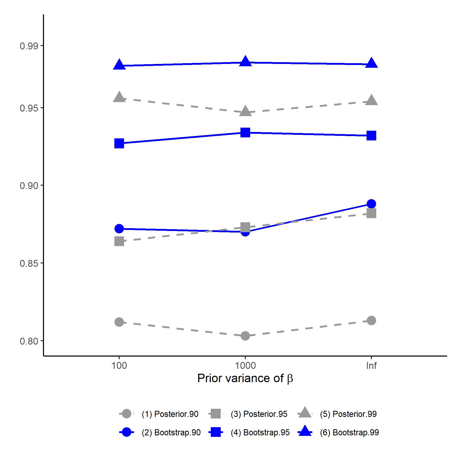
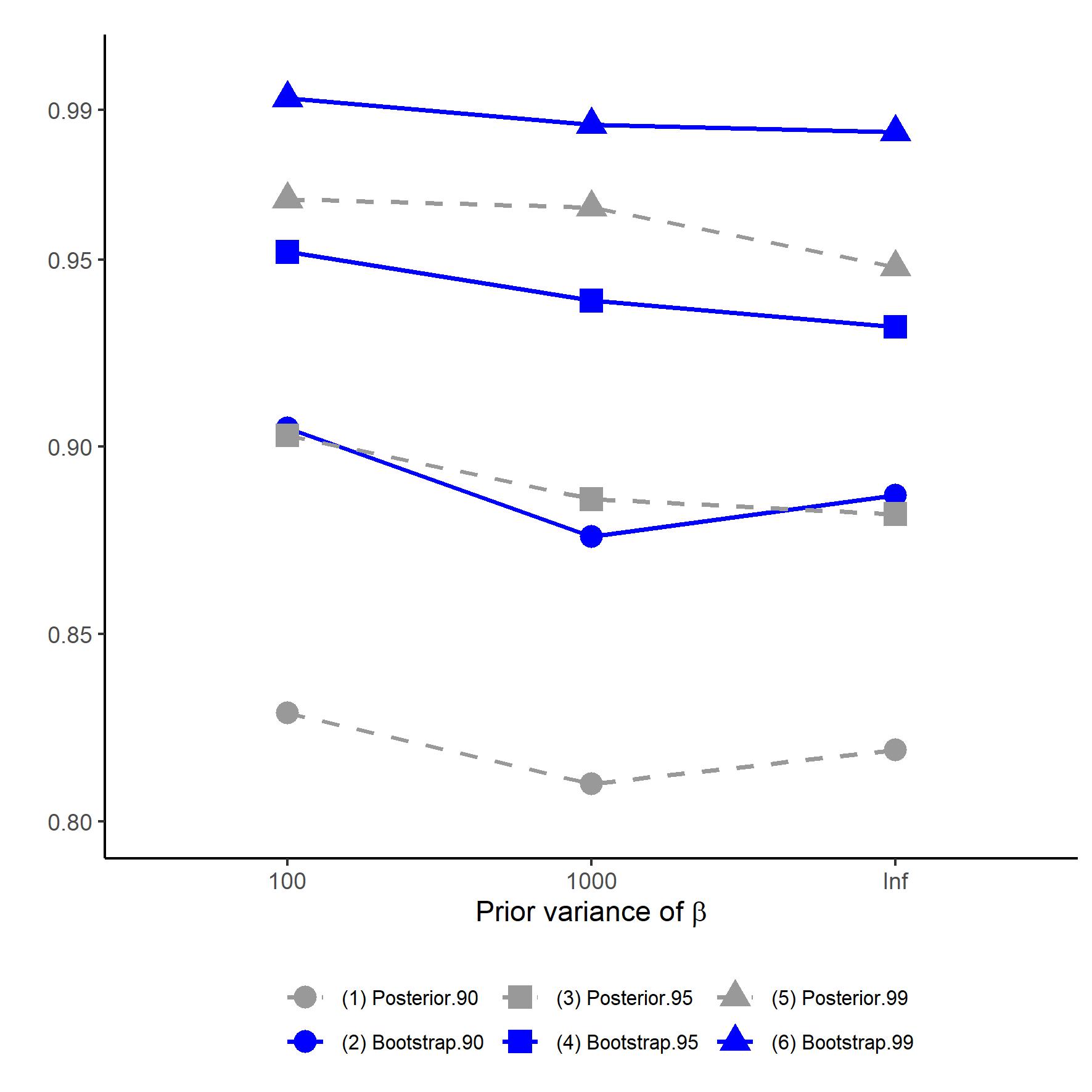
4.2. Empirical Application

We apply the quasi-Bayesian approach to a real dataset about the firms’ incorporation decisions, initially constructed by Eldar and Magnolfi (2020). We focus on the effect of states’ anti-takeover laws on firms’ choice of where to incorporate their business. The data includes an ATS index scoring from $0$ to $5$ that counts the number of anti-takeover statutes in each of $51$ states (including the District of Columbia). Two states dominate the incorporation market in the US: in 2013, $63.9\%$ firms were incorporated in Delaware, and $8.5\%$ in Nevada. Letting $i$ denote firm and $j$ denote the incorporation choice, we consider an MNP model with three choices: Delaware ($j=1$), Nevada ($j=2$), and other states ($j=0$). The regressors contain $ATS$ and its interaction with firm-level characteristics. We use the data in the year 2013, which contains 2,922 firms. We specify the firm’s latent utility as follows:

(4.3) $$U_{ij} = \tilde{\beta}_{1}ATS_{j}+(ATS_{j}\times X_{i})^{\top}\tilde{\beta}_{2}+\varepsilon_{ij},~{}~{}~{}j=0,1,2.$$

where $X_{i}$ is a vector of firm characteristics: share of institutional ownership ($Institutional$ $ownership$), dummies for small and median-sized firms ($small$ and $medium$), and takeover premium ($premium$) in the industry. The main concern for the endogeneity arises from institutional ownership. Following Eldar and Magnolfi (2020), we use the dummy instrumental variable S&P 500 that indicates whether the firm is included in the S&P 500 index. Inclusion in the S&P 500 index is positively correlated with a firm’s institutional ownership. On the other hand, S&P 500 is mainly decided by the market’s view about the firm’s representativeness and thus does not depend on the firms’ decisions. The first-stage is

(4.4) $$Institutional~{}ownership_{i} = \zeta(S\&P500,X_{-1i})+v_{i},$$

where $\zeta$ is an unknown function and $X_{-1i}=\{Small_{i},Medium_{i},Premium_{i}\}$. The control function $v_{i}$ decomposes the error term in (4.3) by $\varepsilon_{ij}=\lambda_{j}v_{i}+\epsilon_{ij}$. We estimate the first stage (4.4) by a kernel regression and then draw the posteriors of $\tilde{\beta}_{1}$ and $\tilde{\beta}_{2}$ in the same way as our simulation exercise. The point estimates in Table 2 are posterior means, and the $95\%$ confidence intervals reported in brackets are constructed using bootstrap. The significantly negative estimate for $\tilde{\beta}_{1}$ suggests that firms on average prefer less legal restrictions on the takeover. Moreover, such preference is heterogeneous in firm characteristics. In particular, small firms are more likely to welcome the anti-takeover laws, which explains why Nevada, with $ATS=5$, occupies a notable market share for incorporation. Our results align with the findings of Eldar and Magnolfi (2020), who estimated a multinomial logit model.

Table 2. Quasi-Bayesian estimates for incorporation decision, bootstrapped $95\%$ confidence intervals in brackets, $n=2,922$.

$ATS$	-0.065
	[-0.108, -0.018]
$ATS\times Institutional~{}ownership$	-0.253
	[-0.311, -0.200]
$ATS\times Small$	0.080
	[0.024, 0.127]
$ATS\times Medium$	-0.005
	[-0.040, 0.030]
$ATS\times Premium$	-0.043
	[-0.072, -0.012]

5. Conclusion

Our research highlights two key aspects of modern econometric models. Firstly, the complexity of these models leads to analytically intractable likelihoods, which can be more conveniently dealt with by simulation-based procedures like the Bayesian method. Secondly, the control function approach effectively handles the endogeneity problem by including the first-stage residuals as additional covariates, rectifying the second stage’s inconsistency. Our study extensively investigates this novel quasi-Bayesian method. Given the widespread use of the Bayesian approach in contemporary econometrics and machine learning, our method provides practitioners with enhanced flexibility to integrate cutting-edge algorithms from various estimation stages. This methodology can be beneficial for other structural models when the general theory is well understood.

6. Appendix A: Proofs of Main Results

Proof of Theorem 2.1.

Our proof of (2.3) is patterned in line with generic arguments in the proof of Theorem 1.4.2 from Ghosh and Ramamoorthi (2002) or Theorem 1 from Chernozhukov and Hong (2003). The crux is to address the first-stage nonparametric estimator $\widehat{\zeta}_{n}$. This is reflected in a different choice of splitting ranges of the integration and a more delicate expansion of the quasi-log-likelihood ratio in our proof.

Consider the following normalized quasi-posterior distribution of $h\equiv\sqrt{n}(\theta-\widehat{\theta}_{n})$:

$$\tilde{\pi}(h|\bm{Y}_{2}^{n};\widehat{\zeta}_{n})= \frac{\prod_{i=1}^{n}p_{\widehat{\theta}_{n}+\frac{h}{\sqrt{n}}}(Y_{2,i}|\widehat{\zeta}_{n})\pi(\widehat{\theta}_{n}+\frac{h}{\sqrt{n}})}{\int\prod_{i=1}^{n}p_{\widehat{\theta}_{n}+\frac{h}{\sqrt{n}}}(Y_{2,i}|\widehat{\zeta}_{n})\pi(\widehat{\theta}_{n}+\frac{h}{\sqrt{n}})dh}$$

$$= \frac{\prod_{i=1}^{n}\left[p_{\widehat{\theta}_{n}+\frac{h}{\sqrt{n}}}(Y_{2,i}|\widehat{\zeta}_{n})/p_{\widehat{\theta}_{n}}(Y_{2,i}|\widehat{\zeta}_{n})\right]\pi(\widehat{\theta}_{n}+\frac{h}{\sqrt{n}})}{\int\prod_{i=1}^{n}\left[p_{\widehat{\theta}_{n}+\frac{h}{\sqrt{n}}}(Y_{2,i}|\widehat{\zeta}_{n})/p_{\widehat{\theta}_{n}}(Y_{2,i}|\widehat{\zeta}_{n})\right]\pi(\widehat{\theta}_{n}+\frac{h}{\sqrt{n}})dh}.$$

Denote its denominator as

(6.1) $$C_{n}\equiv\int\prod_{i=1}^{n}\left[\frac{p_{\widehat{\theta}_{n}+\frac{h}{\sqrt{n}}}(Y_{2,i}|\widehat{\zeta}_{n})}{p_{\widehat{\theta}_{n}}(Y_{2,i}|\widehat{\zeta}_{n})}\right]\pi(\widehat{\theta}_{n}+\frac{h}{\sqrt{n}})dh.$$

Recall that the limiting normal probability density function is as follows:

$$\pi_{\infty}(h)\equiv(2\pi)^{-p/2}|\det V_{0}|^{1/2}\exp\left\{-\frac{h^{\top}V_{0}h}{2}\right\}.$$

The total variation norm we employ can be bounded from above by

$$\int|h|^{a}\left|\tilde{\pi}(h|\bm{Y}_{2}^{n};\widehat{\zeta}_{n})-\pi_{\infty}(h)\right|dh$$

$$\leq C_{n}^{-1}\underbrace{\int|h|^{a}\left|\prod_{i=1}^{n}\left[\frac{p_{\widehat{\theta}_{n}+\frac{h}{\sqrt{n}}}(Y_{2,i}|\widehat{\zeta}_{n})}{p_{\widehat{\theta}_{n}}(Y_{2,i}|\widehat{\zeta}_{n})}\right]\pi(\widehat{\theta}_{n}+\frac{h}{\sqrt{n}})-e^{-\frac{h^{\top}V_{0}h}{2}}\pi(\theta_{0})\right|dh}_{N_{n1}}$$

(6.2) $$+ C_{n}^{-1}\underbrace{\int|h|^{a}e^{-\frac{h^{\top}V_{0}h}{2}}\left(\pi(\theta_{0})-C_{n}(2\pi)^{-p/2}\left|\det V_{0}\right|^{1/2}\right)dh}_{N_{n2}}.$$

It is sufficient to show that

(6.3) $$N_{n1}\equiv\int|h|^{a}\left|\prod_{i=1}^{n}\left[\frac{p_{\widehat{\theta}_{n}+\frac{h}{\sqrt{n}}}(Y_{2,i}|\widehat{\zeta}_{n})}{p_{\widehat{\theta}_{n}}(Y_{2,i}|\widehat{\zeta}_{n})}\right]\pi(\widehat{\theta}_{n}+\frac{h}{\sqrt{n}})-e^{-\frac{h^{\top}V_{0}h}{2}}\pi(\theta_{0})\right|dh=o_{P_{0}}(1).$$

This is because if (6.3) holds, taking $a=0$ leads to

(6.4) $$C_{n}=(2\pi)^{p/2}\left|\det V_{0}\right|^{-1/2}\pi(\theta_{0})+o_{P_{0}}(1),$$

which yields $C_{n}=O_{P_{0}}(1)$. The convergence in (6.4) also implies

$$N_{n2}=\left|C_{n}(2\pi)^{-p/2}|\det V_{0}|^{1/2}-\pi(\theta_{0})\right|\int_{\mathbb{R}^{p}}|h|^{a}\exp\left\{-\frac{h^{\top}V_{0}h}{2}\right\}dh=o_{P_{0}}(1),$$

which makes the upper bound in (6.2) for the total variation norm satisfy $(N_{n1}+N_{n2})/C_{n}=o_{P_{0}}(1)$. This completes the proof of 2.3.

To show (6.3), we split its integration range into three mutually exclusive areas:

• $H_{1,n}\equiv\{h:|h|\leq C\sqrt{n}r_{n}\}$;

• $H_{2,n}\equiv\{h:Cr_{n}\sqrt{n}<|h|\leq\delta\sqrt{n}\}$;

• $H_{3,n}\equiv\{h:|h|>\delta\sqrt{n}\}$;

for a large positive constant $C$ and a small $\delta>0$ to be specified in the sequel. Note that

$$\int_{H_{2,n}\cup H_{3,n}}\exp\left(-\frac{h^{\top}V_{0}h}{2}\right)\pi(\theta_{0})dh=o(1),$$

given the fact that the smallest eigenvalue of $V_{0}$ is positive and $r_{n}\sqrt{n}\to\infty$. We further define

(6.5) $$\Delta_{n}^{r}\equiv\sup_{d_{\Theta}(\theta,\theta_{0})\geq r}\left\{\frac{1}{n}\sum_{i=1}^{n}[\log p_{\theta}(Y_{2i};\widehat{\zeta}_{n})-\log p_{\widehat{\theta}_{n}}(Y_{2i};\widehat{\zeta}_{n})]\right\}.$$

First consider the integration over the outer range $H_{3,n}$. By Lemma 7.1, for any small $\epsilon>0$, we have

(6.6) $$\int_{H_{3,n}}|h|^{a}\prod_{i=1}^{n}\frac{p_{\widehat{\theta}_{n}+\frac{h}{\sqrt{n}}}(Y_{2,i}|\widehat{\zeta}_{n})}{p_{\widehat{\theta}_{n}}(Y_{2,i}|\widehat{\zeta}_{n})}\pi(h)dh\leq\mathbb{I}\{\Delta_{n}^{\delta}<-\epsilon\}\sqrt{n}^{a+1}e^{-n\epsilon}\int_{\theta\in\Theta}|\theta|^{a}\pi(\theta)d\theta,~{}w.p.a.1.$$

The right hand side of the above inequality is of $o_{P_{0}}(1)$.

Then consider the integration over the middle range $H_{2,n}$. Applying Lemma 7.2, we have

$$\int_{H_{2,n}}|h|^{a}\prod_{i=1}^{n}\frac{p_{\widehat{\theta}_{n}+\frac{h}{\sqrt{n}}}(Y_{2,i}|\widehat{\zeta}_{n})}{p_{\widehat{\theta}_{n}}(Y_{2,i}|\widehat{\zeta}_{n})}\pi(h)dh\leq\mathbb{I}\{\Delta_{n}^{Cr_{n}}<-cr_{n}^{2}\}\sqrt{n}^{a+1}e^{-cnr_{n}^{2}}\int_{\theta\in\Theta}|\theta|^{a}\pi(\theta)d\theta,$$

for any given positive $c$ and a large enough constant $C$, $w.p.a.1$. The right hand side of the above inequality is again of $o_{P_{0}}(1)$.

Lastly, we consider the inner range $H_{1,n}$. We first switch from $\pi(\theta_{0})$ to $\pi(\widehat{\theta}_{n}+h/\sqrt{n})$ by noting that $\sup_{h\in\mathcal{H}_{n}}\limsup\left|\widehat{\theta}_{n}+\frac{h}{\sqrt{n}}-\theta_{0}\right|=o_{P_{0}}(1)$, which implies

$$\int_{H_{1,n}}|h|^{a}\exp\left(-\frac{h^{\top}V_{0}h}{2}\right)\left|\pi(\widehat{\theta}_{n}+\frac{h}{\sqrt{n}})-\pi(\theta_{0})\right|dh=o_{P_{0}}(1),$$

by the continuity of the prior density $\pi(\cdot)$ and the dominated convergence. The remaining analysis is about

$$\int_{H_{1,n}}|h|^{a}\left|\prod_{i=1}^{n}\left[\frac{p_{\widehat{\theta}_{n}+\frac{h}{\sqrt{n}}}(Y_{2,i}|\widehat{\zeta}_{n})}{p_{\widehat{\theta}_{n}}(Y_{2,i}|\widehat{\zeta}_{n})}\right]-\exp\left(-\frac{h^{\top}V_{0}h}{2}\right)\right|\pi(\widehat{\theta}_{n}+\frac{h}{\sqrt{n}})dh$$

$$=\int_{H_{1,n}}|h|^{a}e^{-\frac{1}{2}h^{\top}V_{0}h}\left|\exp\left\{\sum_{i=1}^{n}\log p_{\widehat{\theta}_{n}+\frac{h}{\sqrt{n}}}(Y_{2,i}|\widehat{\zeta}_{n})-\log p_{\widehat{\theta}_{n}}(Y_{2,i}|\widehat{\zeta}_{n})+\frac{1}{2}h^{\top}V_{0}h\right\}-1\right|\pi(\widehat{\theta}_{n}+\frac{h}{\sqrt{n}})dh$$

$$\leq A_{n}\times B_{n},$$

where

$$A_{n} \equiv\int_{\mathcal{H}_{1,n}}|h|^{a}\exp\left\{-\frac{h^{\top}V_{0}h}{4}\right\}\pi(\widehat{\theta}_{n}+\frac{h}{\sqrt{n}})dh,$$

$$B_{n} \equiv\sup_{h\in H_{1,n}}\left[e^{-\frac{1}{4}h^{\top}V_{0}h}\left|\exp\left\{\sum_{i=1}^{n}\log p_{\widehat{\theta}_{n}+\frac{h}{\sqrt{n}}}(Y_{2,i}|\widehat{\zeta}_{n})-\log p_{\widehat{\theta}_{n}}(Y_{2,i}|\widehat{\zeta}_{n})+\frac{1}{2}h^{\top}V_{0}h\right\}-1\right|\right].$$

It is clear that $A_{n}$ is stochastically bounded due to the boundedness of the prior density. Lemma 7.4 shows $B_{n}=o_{P_{0}}(1)$. Then we obtain $A_{n}\times B_{n}=o_{P_{0}}(1)$, which completes the proof of (6.3).

The convergence in the norm $TVM(a)$ stated in (2.3) immediately implies the convergence of the distribution in the total variation as stated in (2.4); see Ghosh and Ramamoorthi (2002). ∎

Proof of Corollary 2.1.

We denote the $p$-dimensional standard normal measure of a generic set $A$ by $\mathbb{N}(A)\equiv(2\pi)^{-p/2}\int_{A}e^{-h^{\top}h/2}dh$. Recall the definition of $\Delta_{n,0}$ in Assumption 2.8. Consider the quasi-Bayesian credible set $\mathcal{C}_{n}(\alpha)$, which satisfies $\Pi(\theta\in\mathcal{C}_{n}(\alpha)|{\bm{Y}}_{2}^{n},\widehat{\zeta}_{n})=1-\alpha$. Applying (2.3) in Theorem 2.1 with $a=0$ and using (7.2) in Appendix B, we have

$$\mathbb{N}(V_{0}^{1/2}n^{1/2}(\mathcal{C}_{n}(\alpha)-\theta_{0}-n^{-1/2}V_{0}^{-1}\Delta_{n,0}))\to 1-\alpha~{}~{}\text{in probability}.$$

Thus, $\mathcal{C}_{n}(\alpha)=\theta_{0}+n^{-1/2}V_{0}^{-1}\Delta_{n,0}+n^{-1/2}V_{0}^{-1/2}B_{n}$, where $B_{n}$ satisfies $\mathbb{N}(B_{n})\to 1-\alpha$, as $n\to\infty$. Therefore, the frequentist coverage of the Bayesian credible set is

$$P_{0}\{\theta_{0}\in\mathcal{C}_{n}(\alpha)\}=P_{0}\{\theta_{0}\in\theta_{0}+n^{-1/2}V_{0}^{-1}\Delta_{n,0}+n^{-1/2}V_{0}^{-1/2}B_{n}\}=P_{0}\{-V_{0}^{-1/2}\Delta_{n,0}\in B_{n}\}.$$

The above coverage probability of the set $\mathcal{C}_{n}(\alpha)$ does not converge to $1-\alpha$ in general, unless the matrix $V_{0}$ is equal to $\Omega_{0}$, which is the asymptotic covariance matrix of $\Gamma_{1}(Y_{1})+\Gamma_{2}(Y_{2})$ in our Assumption 2.8. ∎

Proof of Corollary 2.2.

The convergence in the total variation of moments norm with $a=1$ implies that

$$\int h\left(\tilde{\pi}(h|\bm{Y}_{2}^{n};\widehat{\zeta}_{n})-\pi_{\infty}(h)\right)dh\to_{P_{0}}0.$$

As the limiting normal distribution is centered around zero, i.e., $\int h\pi_{\infty}(h)dh=0$, we have

$$\int h\tilde{\pi}(h|\bm{Y}_{2}^{n};\widehat{\zeta}_{n})dh\to_{P_{0}}0.$$

Translating the above result to the quasi-posterior mean, we note that

$$\widetilde{\theta}_{n}\equiv\int\theta d\Pi_{n}(\theta|\bm{Y_{2}};\widehat{\zeta}_{n})=\int\left(\widehat{\theta}_{n}+\frac{h}{\sqrt{n}}\right)\tilde{\pi}(h|\bm{Y}_{2}^{n};\widehat{\zeta}_{n})dh=\widehat{\theta}_{n}+o_{P_{0}}(n^{-1/2}),$$

which leads to the desired result. The proof of the posterior variance follows along similar lines involving the second-order moment. It is straightforward and hence omitted. ∎

Proof of Theorem 2.2.

In Lemma 7.5, we have shown the convergence in total variation norm for the bootstrapped posterior density function. This implies the asymptotic equivalence of the mean of the bootstrapped quasi-posterior $\widetilde{\theta}^{*}_{n}$ and the bootstrap frequentist-type two-stage estimator $\widehat{\theta}_{n}^{*}$, i.e., $\sqrt{n}\left(\widetilde{\theta}_{n}^{*}-\widehat{\theta}^{*}_{n}\right)$ is $o_{P^{*}}(1)$. For the two-stage frequentist estimators, we have the following:

(6.7) $$\sup_{\xi\in\mathbb{R}^{p}}|P_{0}(\sqrt{n}(V_{0}\Omega_{0}V_{0})^{-1/2}(\widehat{\theta}_{n}-\theta_{0})\leq\xi)-\Phi_{p}(\xi)|\to_{P_{0}}0,$$

and its bootstrap analog:

(6.8) $$\sup_{\xi\in\mathbb{R}^{p}}|P^{*}(\sqrt{n}(V_{0}\Omega_{0}V_{0})^{-1/2}(\widehat{\theta}^{*}_{n}-\widehat{\theta}_{n})\leq\xi)-\Phi_{p}(\xi)|\to_{P^{*}}0.$$

Using (6.7), (6.8), and the asymptotic equivalence between $\widetilde{\theta}_{n}^{*}$ and $\widehat{\theta}^{*}_{n}$, we conclude the proof by applying Corollary 1 in Cheng and Huang (2010). ∎

Proof of Proposition 3.1.

We verify the high-level assumptions that lead to our Theorems 2.1 and 2.2. Regarding Assumption 2.1, we have a well-separated maximum point, due to the identification and the compactness of the parameter space in Assumption 3.1, as well as the continuity of the log-likelihood function (Newey and McFadden, 1994). Assumption 3.3 also satisfies the convergence rate condition in Assumption 2.2. Referring to the frequentist’s estimator $\widehat{\theta}_{n}$, one can take the simulated score estimator by Hajivassiliou and McFadden (1998) in the second stage. The prior specification given in Assumption 3.4 satisfies the requirement in Assumption 2.4. The normality of the error term generates sufficient smoothness of the conditional choice probabilities, which satisfy Assumption 2.6. Therein, the function $e_{n}(\cdot,\cdot)$ in Assumption 2.5 can be taken as the cross product term $(\theta-\theta_{0})^{\top}\mathbb{E}[\ddot{l}_{\theta,\zeta}][\zeta-\zeta_{0}]$ as in Lemma C.2 of Chen, Lee, and Sung (2014). The smoothness of MNP implies a stronger notion of differentiability than what is required in Assumption 2.6, i.e., the likelihood is Frechét differentiable w.r.t. $\zeta$ (Ichimura and Lee, 2010).

To verify Assumption 2.7, recall that the bracketing number $N_{\left[{}\right]}\left(\epsilon,\mathcal{F},\left\|\cdot\right\|_{2}\right)$ for a functional class $\mathcal{F}$ is defined to be the minimum of $m$ such that $\exists$ $f_{1}^{L},f_{1}^{U},\dots,f_{m}^{L},f_{m}^{U}$ for $\forall f\in\mathcal{F}$, $f_{j}^{L}\leq f\leq f_{j}^{U}$ for some $j$, and $\left\|f_{j}^{U}-f_{j}^{L}\right\|_{2}\leq\epsilon$ (van der Vaart and Wellner, 1996). Let $\mathcal{P}\equiv\{\log p_{\theta}(Y_{2i};\zeta):\theta\in\Theta,\zeta\in\mathcal{G}_{n}\}$. Our Assumption 3.2 on the Hölder class implies the $P_{0}$-Glivenko-Cantelli property of $\mathcal{P}$. Given the smoothness requirement in Assumption 3.2, we can utilize the Lipschitz continuity and apply Theorem 2.7.11 and Theorem 2.7.1 in van der Vaart and Wellner (1996) to bound its overall entropy by

(6.9) $$\log N_{\left[{}\right]}(\epsilon,\mathcal{P},\left\|\cdot\right\|_{2})\lesssim\log N_{\left[{}\right]}(\epsilon/2C,\Theta,\left\|\cdot\right\|_{2})+\log N_{\left[{}\right]}(\rho/2C,\mathcal{G}_{n},\left\|\cdot\right\|_{2})\lesssim p\log(\epsilon^{-1})+\epsilon^{-d/\tau}.$$

To check the $P_{0}$-Donsker property as in Assumption 2.7(ii), we follow the route in Example 19.7 from van der Vaart (1998) given our Assumption 3.5, along with the restriction that $\tau>d/2$ in Assumption 3.2. Other properties, such as the functional class of the second derivative $\ddot{l}_{\theta}$ being $P_{0}$-Glivenko-Cantelli, can be checked along similar lines, utilizing the smoothness of the MNP in the second stage, as well as the entropy bound for the Hölder class from the first stage in (6.9); see McFadden (1989) and Pakes and Pollard (1989). The score functions of $\beta$ and $\eta$ (equations (14) and (15) in Hajivassiliou and McFadden (1998)) have finite second-order moments given the bounded support of covariates and control variables. Given the smoothness and boundedness of covariates suppport, we also have the envelope functions being bounded. Thus, the slightly strong assumption used in the bootstrap part is also satisfied. When it comes to Assumption 2.7(iii), one can apply Lemma 2.14.3 in van der Vaart and Wellner (1996) to obtain $\phi_{n}(\rho)=\rho^{1-\frac{d}{2\tau}}$, which satisfy the restrictions under the maintained assumption $\tau>d/2$. By equation (3.15) of Ichimura and Lee (2010), the influence function of the first-stage estimation defined by $\Gamma_{1}(Y_{1i})=\sum_{j=0}^{J}\int\phi_{n,j}(\cdot,\theta_{0})\frac{\partial g_{j}(\cdot,\theta_{0})}{\partial\theta}dP_{0}$. The asymptotic normality in Assumption 2.8 follows from the Lindeberg-Lévy CLT under Assumption 3.6. ∎

7. Appendix B: Proofs of Technical Lemmas

We prove several technical lemmas needed in the proof of Theorems 2.1 and 2.2 in this part. For simplicity, we state the lemmas under all of our maintained Assumptions 2.1 to 2.8. From the proofs, it is clear which specific conditions are actually invoked.

Lemma 7.1.

Under Assumptions 2.1 to 2.8, for any $\delta>0$, we have the following inequality holds w.p.a.1,

(7.1) $$\sup_{d_{\Theta}(\theta,\theta_{0})>\delta}\mathbb{P}_{n}[\log p_{\theta}(Y_{2i};\widehat{\zeta}_{n})-\log p_{\widehat{\theta}_{n}}(Y_{2i};\widehat{\zeta}_{n})]\leq-c,$$

for some positive constant term $c$.

Proof.

We start with the following decomposition:

$$\mathbb{P}_{n}[\log p_{\theta}(Y_{2i};\widehat{\zeta}_{n})-\log p_{\widehat{\theta}_{n}}(Y_{2i};\zeta_{0})]$$

$$= \mathbb{P}_{n}[\log p_{\theta}(Y_{2i};\widehat{\zeta}_{n})-\log p_{\theta_{0}}(Y_{2i};\zeta_{0})]+\mathbb{P}_{n}[\log p_{\theta_{0}}(Y_{2i};\zeta_{0})-\log p_{\widehat{\theta}_{n}}(Y_{2i};\widehat{\zeta}_{n})].$$

The second term above can be shown to be $o_{P_{0}}(1)$ following the standard consistency argument for the two-stage estimation given the identification in Assumption 2.1 and $P_{0}$-Glivenko-Cantelli property in Assumption 2.7; see Chen (2007). Therefore, we focus on the first term and decompose it as follows:

$$\mathbb{P}_{n}[\log p_{\theta}(Y_{2i};\widehat{\zeta}_{n})-\log p_{\theta_{0}}(Y_{2i};\zeta_{0})]$$

$$= (\mathbb{P}_{n}-P_{0})[\log p_{\theta}(Y_{2i};\widehat{\zeta}_{n})]-(\mathbb{P}_{n}-P_{0})[\log p_{\theta_{0}}(Y_{2i};\zeta_{0})]$$

$$+ P_{0}[\log p_{\theta}(Y_{2i};\widehat{\zeta}_{n})-\log p_{\theta}(Y_{2i};\zeta_{0})]+P_{0}[\log p_{\theta}(Y_{2i};\zeta_{0})-\log p_{\theta_{0}}(Y_{2i};\zeta_{0})].$$

By the $P_{0}$-Glivenko-Cantelli property, i.e., $\sup_{\theta\in\Theta,\zeta\in\mathcal{G}_{n}}\left|(\mathbb{P}_{n}-P_{0})[\log p_{\theta}(Y_{2i};\zeta)]\right|=o_{P_{0}}(1)$, we have the first two terms on the right hand side of the above equality converging to zero in probability uniformly for any $\theta\in\Theta$. When it comes to the third term, we utilize the uniform (regarding $\theta$) continuity of the criterion function with respect to the first stage nuisance function in our Assumption 2.6, so that $P_{0}[\log p_{\theta}(Y_{2i};\widehat{\zeta}_{n})-\log p_{\theta}(Y_{2i};\zeta_{0})]=o_{P_{0}}(1)$. For any given $\delta>0$, the last term satisfies

$$\sup_{d_{\Theta}(\theta,\theta_{0})>\delta}\left|P_{0}\left[\log p_{\theta}(\cdot;\zeta_{0})-\log p_{\theta_{0}}(\cdot;\zeta_{0})\right]\right|\leq-c,$$

with a proper choice of constant $c>0$, which concludes the proof. ∎

Our assumptions imply Conditions (i)-(iv) in Corollary 1 of Nan and Wellner (2013). Thus, the frequentist’s two-stage estimator satisfies the following expansion:

$$(\widehat{\theta}_{n}-\theta_{0}) =-V_{0}^{-1}\left(S_{\theta,n}(\theta_{0},\zeta_{0})+\dot{\Psi}_{\zeta}(\theta_{0},\zeta_{0})[\widehat{\zeta}_{n}-\zeta_{0}]\right)+o_{P_{0}}(n^{-1/2})$$

(7.2) $$\equiv-V_{0}^{-1}\frac{1}{\sqrt{n}}\sum_{i=1}^{n}\left[\Gamma_{2}(Y_{2i})+\Gamma_{1}(Y_{1i})\right]+o_{P_{0}}(n^{-1/2}),$$

which implies that $\widehat{\theta}_{n}$ is root-$n$ consistent and asymptotically normal.

Lemma 7.2.

Recall the definition of $\Delta_{n}^{r}$ in (6.5). Under Assumptions 2.1 to 2.8, for the decreasing sequence $r_{n}=o(n^{-1/4})$ and $nr^{2}_{n}\to\infty$, we have

(7.3) $$\lim\sup_{n\to\infty}P_{0}\{\Delta_{n}^{Cr_{n}}\geq-cr_{n}^{2}\}=0,$$

for a given positive $c$ and a large enough positive constant $C$.

Proof of Lemma 7.2.

Because $\widehat{\theta}_{n}$ is root-$n$ consistent and $nr^{2}_{n}\to\infty$, we have

$$\{\theta:d_{\Theta}(\theta,\widehat{\theta}_{n})\geq Cr_{n}\}\subset\{\theta:d_{\Theta}(\theta,\theta_{0})\geq C^{\prime}r_{n}\},$$

for a proper choice of the constant term $C^{\prime}$. Therefore, we obtain

$$\{\Delta_{n}^{C^{r}_{n}}\geq-cr_{n}^{2}\} \subset\{\sup_{\theta:d_{\Theta}(\theta,\theta_{0})\geq C^{\prime}r_{n}}\mathbb{P}_{n}[\log p_{\theta}(Y_{2};\widehat{\zeta}_{n})-\log p_{\widehat{\theta}_{n}}(Y_{2};\widehat{\zeta}_{n})]\geq-cr^{2}_{n}\}$$

$$\subset\{\sup_{\theta:d_{\Theta}(\theta,\theta_{0})\geq C^{\prime}r_{n}}\mathbb{P}_{n}[\log p_{\theta}(Y_{2};\widehat{\zeta}_{n})-\log p_{\theta_{0}}(Y_{2};\widehat{\zeta}_{n})]\geq-cr^{2}_{n}\},$$

where the second inclusion follows from $\mathbb{P}_{n}[\log p_{\widehat{\theta}_{n}}(Y_{2};\widehat{\zeta}_{n})]\geq\mathbb{P}_{n}[\log p_{\theta_{0}}(Y_{2};\widehat{\zeta}_{n})]$ by definition of $\widehat{\theta}_{n}$ from Assumption 2.3. We can further restrict to our attention to the set $B_{n}\equiv\{d_{G}(\zeta,\zeta_{0})\leq Cr_{n}\}$, as its complement is asymptotically negligible by Assumption 2.2. It suffices to examine

(7.4) $$\left\{\sup_{d_{\Theta}(\theta,\theta_{0})\geq C^{\prime}r_{n},d_{G}(\zeta,\zeta_{0})\leq Cr_{n}}\mathbb{P}_{n}[\log p_{\theta}(Y_{2};\zeta)-\log p_{\theta_{0}}(Y_{2};\zeta)]\geq-cr^{2}_{n}\right\}$$

Thanks to our Lemma 7.1, we can localize on the set $\{\theta:d_{\Theta}(\theta,\theta_{0})\leq\delta\}$ for a given small $\delta$. This localized set will be partitioned into the shells for $\rho=C^{\prime}r_{n}$:

$$S_{n,j,M}=\left\{(\theta,\zeta)\in\Theta_{n}\times\mathcal{G}_{n}:2^{j-1}\rho<d_{\Theta}(\theta,\theta_{0})\leq 2^{j}\rho,d_{G}(\zeta,\zeta_{0})\leq 2^{-M}d_{\Theta}(\theta,\theta_{0})\right\}.$$

In the slicing argument, we sum over the shells that $2^{j}\rho<\delta$. For the $j$-th set involved, we have

$$P_{0}(\log p_{\theta}(Y_{2};\zeta)-\log p_{\theta_{0}}(Y_{2};\zeta))$$

$$= P_{0}(\log p_{\theta}(Y_{2};\zeta)-\log p_{\theta_{0}}(Y_{2};\zeta_{0}))+P_{0}(\log p_{\theta_{0}}(Y_{2};\zeta_{0})-\log p_{\theta_{0}}(Y_{2};\zeta))$$

$$\leq P_{0}(\log p_{\theta}(Y_{2};\zeta)-\log p_{\theta_{0}}(Y_{2};\zeta_{0}))+e_{n}(\theta,\zeta)+C_{1}r_{n}^{2}$$

(7.5) $$\lesssim -d_{\Theta}^{2}(\theta,\theta_{0})+d^{2}_{G}(\zeta,\zeta_{0})+C_{2}2^{j}\rho r_{n}+C_{1}r_{n}^{2}\lesssim-(1-2^{-2M})d_{\Theta}^{2}(\theta,\theta_{0})\lesssim-2^{2j-2}\rho^{2},$$

under Assumption 2.5. In other words, we have

$$\inf_{(\theta,\zeta)\in S_{n,j,M}}-P_{0}(\log p_{\theta}(Y_{2};\zeta)-\log p_{\theta_{0}}(Y_{2};\zeta))\geq 2^{2j-2}\rho^{2}.$$

Thus, the probability of (7.4) can be bounded by

$$\sum_{j\geq M,2^{j}\rho_{n}\leq\delta}P_{0}\left(\sup_{(\theta,\zeta)\in S_{n,j,M}}\mathbb{P}_{n}[\log p_{\theta}(Y_{2};\zeta)-\log p_{\theta_{0}}(Y_{2};\zeta)]\geq-c_{1}r_{n}^{2}\right)$$

$$\leq\sum_{j\geq M}P_{0}\left(\sup_{(\theta,\zeta)\in S_{n,j,M}}\mathbb{G}_{n}[\log p_{\theta}(Y_{2};\zeta)-\log p_{\theta_{0}}(Y_{2};\zeta)]\geq C2^{2j-2}\sqrt{n}\rho^{2}\right)$$

$$\lesssim\sum_{j\geq M}\frac{1}{2^{2j}\sqrt{n}\rho^{2}}\mathbb{E}_{0}\sup_{(\theta,\zeta)\in S_{n,j,M}}\left|\mathbb{G}_{n}[\log p_{\theta}(Y_{2};\zeta)-\log p_{\theta_{0}}(Y_{2};\zeta)]\right|$$

$$\lesssim\sum_{j\geq M}\frac{1}{2^{2j}\sqrt{n}\rho^{2}}\phi_{n}(2^{j}\rho)\leq\sum_{j\geq M}\frac{1}{2^{2j}\sqrt{n}\rho^{2}}2^{j\gamma}\phi_{n}(\rho)\lesssim\sum_{j\geq M}2^{j(\gamma-2)}.$$

In the first inequality, we add/subtract $P_{0}[\log p_{\theta}(\cdot;\zeta)-\log p_{\theta_{0}}(\cdot;\zeta)]$ and apply (7). The fourth inequality makes use of the monotonicity of the mapping $\delta\mapsto\phi_{n}(\delta)/\delta^{\gamma}$ for some $\gamma<2$, so that we have $\phi_{n}(2^{j}\rho)\leq 2^{j\gamma}\phi_{n}(\rho)$. The final inequality follows from $\phi_{n}(\rho)\leq\sqrt{n}\rho^{2}$ for every $n$. The desired result follows by choosing a large enough $M$, which is induced by a large $C$. ∎

Lemma 7.3.

Under Assumptions 2.1 to 2.8, for any $\theta_{n}$ converging to $\theta_{0}$ such that $d_{\Theta}(\theta_{n},\theta_{0})\leq Cr_{n}$ w.p.a.1, one has

(7.6) $$\ell_{n}(\theta_{n};\widehat{\zeta}_{n})-\ell_{n}(\widehat{\theta}_{n};\widehat{\zeta}_{n})=-\frac{1}{2}(\theta_{n}-\widehat{\theta}_{n})^{\top}V_{0}(\theta_{n}-\widehat{\theta}_{n})+o_{P_{0}}(1+\sqrt{n}d_{\Theta}(\theta_{n},\theta_{0}))^{2}.$$

Proof.

Recall that $\Delta_{n,0}\equiv\sqrt{n}\left(S_{\theta,n}(\theta_{0},\zeta_{0})+\dot{\Psi}_{\zeta}(\theta_{0},\zeta_{0})[\widehat{\zeta}_{n}-\zeta_{0}]\right)$. We start with the following string of equations:

$$l_{n}(\theta_{n};\widehat{\zeta}_{n})-l_{n}(\theta_{0};\widehat{\zeta}_{n})$$

$$=n\mathbb{P}_{n}[\log p_{\theta_{n}}(Y_{2};\widehat{\zeta}_{n})-\log p_{\theta_{0}}(Y_{2};\widehat{\zeta}_{n})]$$

$$=\sqrt{n}\mathbb{G}_{n}[\log p_{\theta_{n}}(Y_{2};\widehat{\zeta}_{n})-\log p_{\theta_{0}}(Y_{2};\widehat{\zeta}_{n})]+nP_{0}[\log p_{\theta_{n}}(Y_{2};\widehat{\zeta}_{n})-\log p_{\theta_{0}}(Y_{2};\widehat{\zeta}_{n})]$$

$$=\sqrt{n}\mathbb{G}_{n}\left[\log p_{\theta_{n}}(Y_{2};\widehat{\zeta}_{n})-\log p_{\theta_{0}}(Y_{2};\widehat{\zeta}_{n})-(\theta_{n}-\theta_{0})^{\top}\dot{l}_{\theta}(Y_{2},\theta_{0};\widehat{\zeta}_{n})\right]$$

$$\quad+\sqrt{n}h_{n}^{\top}\mathbb{G}_{n}\left[\dot{l}_{\theta}(Y_{2},\theta_{0};\widehat{\zeta}_{n})-\dot{l}_{\theta}(Y_{2},\theta_{0};\zeta_{0})\right]$$

$$+\sqrt{n}h_{n}^{\top}\mathbb{G}_{n}\left[\dot{l}_{\theta}(Y_{2},\theta_{0};\zeta_{0})\right]+nP_{0}\left[\log p_{\theta_{n}}(Y_{2};\widehat{\zeta}_{n})-\log p_{\theta_{0}}(Y_{2};\widehat{\zeta}_{n})\right]$$

By the $P_{0}$-Donsker property in our Assumption 2.7, we have

(7.7) $$\sup_{d_{\Theta}(\theta_{n},\theta_{0})\leq Cr_{n}}\left|\mathbb{G}_{n}\left[\log p_{\theta_{n}}(Y_{2};\widehat{\zeta}_{n})-\log p_{\theta_{0}}(Y_{2};\widehat{\zeta}_{n})-(\theta_{n}-\theta_{0})^{\top}\dot{l}_{\theta}(Y_{2},\theta_{0};\widehat{\zeta}_{n})\right]\right|=o_{P_{0}}(d_{\Theta}(\theta_{n},\theta_{0})),$$

and

(7.8) $$\mathbb{G}_{n}\left[\dot{l}_{\theta}(Y_{2},\theta_{0};\widehat{\zeta}_{n})-\dot{l}_{\theta}(Y_{2},\theta_{0};\zeta_{0})\right]=o_{P_{0}}(n^{-1/2}).$$

In addition, the smoothness in Assumption 2.6 leads to

$$\sup_{d_{\Theta}(\theta_{n},\theta_{0})\leq Cr_{n}}\biggl{|}nP_{0}\left[\log p_{\theta_{n}}(Y_{2};\widehat{\zeta}_{n})-\log p_{\theta_{0}}(Y_{2};\widehat{\zeta}_{n})\right]$$

$$\quad\quad\quad\quad\quad-\frac{1}{2}(\theta_{n}-\theta_{0})^{\top}V_{0}(\theta_{n}-\theta_{0})-(\theta_{n}-\theta_{0})^{\top}\dot{\Psi}_{\zeta}(\theta_{0},\zeta_{0})[\widehat{\zeta}_{n}-\zeta_{0}]\biggl{|}$$

$$=o_{P_{0}}(1+\sqrt{n}d_{\Theta}(\theta_{n},\theta_{0}))^{2},$$

where $r_{n}=o(n^{-1/4})$. Combining the previous steps, we have

$$\ell_{n}(\theta_{n};\widehat{\zeta}_{n})-\ell_{n}(\theta_{0};\widehat{\zeta}_{n}) =\sqrt{n}(\theta_{n}-\theta_{0})^{\top}\Delta_{n,0}-\frac{n}{2}(\theta_{n}-\theta_{0})^{\top}V_{0}(\theta_{n}-\theta_{0})$$

$$\quad+o_{P_{0}}(1+\sqrt{n}d_{\Theta}(\theta_{n},\theta_{0}))^{2}$$

$$\ell_{n}(\widehat{\theta}_{n};\widehat{\zeta}_{n})-\ell_{n}(\theta_{0};\widehat{\zeta}_{n}) =\frac{n}{2}(\widehat{\theta}_{n}-\theta_{0})^{\top}V_{0}(\widehat{\theta}_{n}-\theta_{0})+o_{P_{0}}(1+\sqrt{n}d_{\Theta}(\widehat{\theta}_{n},\theta_{0}))^{2}.$$

Now we take the difference of the above two equations and utilize the linear representation of $\widehat{\theta}_{n}$ to get

$$\ell_{n}(\theta_{n};\widehat{\zeta}_{n})-\ell_{n}(\widehat{\theta}_{n};\widehat{\zeta}_{n}) =n(\theta_{n}-\theta_{0})^{\top}V_{0}(\widehat{\theta}_{n}-\theta_{0})-\frac{n}{2}(\theta_{n}-\theta_{0})^{\top}V_{0}(\theta_{n}-\theta_{0})$$

$$-\frac{n}{2}(\widehat{\theta}_{n}-\theta_{0})^{\top}V_{0}(\widehat{\theta}_{n}-\theta_{0})+o_{P_{0}}(1+\sqrt{n}d_{\Theta}(\widehat{\theta}_{n},\theta_{0}))^{2}$$

$$=-\frac{1}{2}(\theta_{n}-\widehat{\theta}_{n})^{\top}V_{0}(\theta_{n}-\widehat{\theta}_{n})+o_{P_{0}}(1+\sqrt{n}d_{\Theta}(\theta_{n},\theta_{0}))^{2}.$$

The last step follows from completing the square of $(\theta_{n}-\widehat{\theta}_{n})^{\top}V_{0}(\theta_{n}-\widehat{\theta}_{n})$. ∎

Lemma 7.4.

Let

$$\tilde{B}_{n}(\theta)\equiv e^{-\frac{n}{4}(\theta-\widehat{\theta}_{n})^{\top}V_{0}(\theta-\widehat{\theta}_{n})}\left|e^{\sum_{i=1}^{n}\log p_{\theta}(Y_{2,i}|\widehat{\zeta}_{n})-\log p_{\widehat{\theta}_{n}}(Y_{2,i}|\widehat{\zeta}_{n})+\frac{n}{2}(\theta-\widehat{\theta}_{n})^{\top}V_{0}(\theta-\widehat{\theta}_{n})}-1\right|.$$

Under Assumptions 2.1 to 2.8, we have $B_{n}\equiv\sup_{d(\theta,\theta_{0})\leq Cr_{n}}\tilde{B}_{n}(\theta)=o_{P_{0}}(1)$.

Proof.

For any random sequence $\theta_{n}$ such that $d_{\Theta}(\theta_{n},\widehat{\theta}_{n})\leq Cr_{n}$ for all $n$ and some fixed $C<\infty$, we have

$$\tilde{B}_{n}(\theta_{n})\leq\exp\left\{-\frac{n}{4}(\theta_{n}-\widehat{\theta}_{n})^{\top}V_{0}(\theta_{n}-\widehat{\theta}_{n})\right\}\times\left|\exp\{o_{P_{0}}(1+\sqrt{n}d_{\Theta}(\theta_{n},\theta_{0}))^{2}\}-1\right|,$$

where the remainder term satisfies

$$o_{P_{0}}(1+\sqrt{n}d_{\Theta}(\theta_{n},\theta_{0}))^{2}\leq o_{P_{0}}(1)[(1+\sqrt{n}d_{\Theta}(\theta_{n},\widehat{\theta}_{n}))^{2}+nd(\theta_{0},\widehat{\theta}_{n})^{2}]$$

$$= o_{P_{0}}(1)(1+\sqrt{n}d_{\Theta}(\theta_{n},\widehat{\theta}_{n}))^{2},$$

due to Lemma 7.3. Note that $|e^{x}-1|\leq e^{|x|}$ for any $x$, we can proceed as follows for a given large positive constant $M$:

$$\tilde{B}_{n}(\theta_{n}) \leq\exp\left\{-\frac{n}{4}(\theta_{n}-\widehat{\theta}_{n})^{\top}V_{0}(\theta_{n}-\widehat{\theta}_{n})\right\}\left|\exp\{o_{P_{0}}(1)\}-1\right|\times\mathbb{I}\{\sqrt{n}d_{\Theta}(\theta_{n},\widehat{\theta}_{n})\leq M\}$$

$$+\exp\left\{-\frac{n}{4}(\theta_{n}-\widehat{\theta}_{n})^{\top}V_{0}(\theta_{n}-\widehat{\theta}_{n})+o_{P_{0}}(1)(1+\sqrt{n}d(\theta_{n},\theta_{0}))^{2}\right\}\times\mathbb{I}\{\sqrt{n}d_{\Theta}(\theta_{n},\widehat{\theta}_{n})\geq M\}$$

$$\leq o_{P_{0}}(1)+\exp\left\{\frac{M^{2}}{4}\lambda_{1}(1-o_{P_{0}}(1))\right\}\to\exp\{-\lambda_{1}M^{2}/4\},$$

where $\lambda_{1}$ is the smallest eigenvalue of $V_{0}$ which is strictly positive by our Assumption 2.1. Therefore, $B_{n}=o_{P_{0}}(1)$, as $M$ can be made arbitrarily large. ∎

Lemma 7.5.

Let the bootstrap posterior density function of $h\equiv\sqrt{n}(\theta-\widehat{\theta}^{*}_{n})$ be

(7.9) $$\tilde{\pi}^{*}(h|\bm{Y}_{2}^{n*};\widehat{\zeta}^{*}_{n})\equiv\frac{\prod_{i=1}^{n}p^{M_{ni}}_{\widehat{\theta}^{*}_{n}+\frac{h}{\sqrt{n}}}(\bm{Y}_{2}^{n}|\widehat{\zeta}^{*}_{n})\pi(\widehat{\theta}^{*}_{n}+\frac{h}{\sqrt{n}})}{\int\prod_{i=1}^{n}p^{M_{ni}}_{\widehat{\theta}^{*}_{n}+\frac{h}{\sqrt{n}}}(\bm{Y}_{2}^{n}|\widehat{\zeta}^{*}_{n})\pi(\widehat{\theta}^{*}_{n}+\frac{h}{\sqrt{n}})dh}.$$

In addition to Assumptions 2.1-2.8, we assume that the envelope functions for the functional classes in Parts (i) and (ii) in Assumption (2.7) have finite $2+\iota$ moments, for $\iota>0$. Then, we have the following convergence in total variation norm:

(7.10) $$\|\tilde{\pi}^{*}(h|\bm{Y}_{2}^{n*};\widehat{\zeta}^{*}_{n})-\pi_{\infty}(h)\|_{TVM(a)}=o_{P^{*}}(1).$$

Proof.

The bootstrap version follows along similar lines of the proof of our Theorem 2.1. We highlight two main modifications needed herein.

First, we show the posterior mass outside an shrinking neighborhood around the truth is negligible conditional on the observed data w.p.a.1. Specifically, we need to characterize the order of $\Delta_{n}^{*Cr_{n}}$, where

$$\Delta_{n}^{*Cr_{n}}=\sup_{\theta:d_{\Theta}(\theta,\widehat{\theta}^{*}_{n})\geq Cr_{n}}\mathbb{P}^{*}_{n}[\log p_{\theta}(Y_{2};\widehat{\zeta}^{*}_{n})-\log p_{\widehat{\theta}_{n}^{*}}(Y_{2};\widehat{\zeta}^{*}_{n})].$$

A key step in the chaining argument is to use a proper maximal inequality related to the bootstrap empirical process. For this purpose, we resort to Corollary 1 from Han and Wellner (2019) to obtain

(7.11) $$\mathbb{E}^{*}_{0}\sup_{(\theta,\zeta)\in S_{n,j,M}}\left|\mathbb{G}^{*}_{n}[\log p_{\theta}(Y_{2};\zeta)-\log p_{\theta_{0}}(Y_{2};\zeta)]\right|\leq C\phi_{n}(2^{j}\rho),$$

with the multinomial weights.

Second, when we carry out an expansion of the bootstrap log-likelihood, we need to verify the following stochastic equicontinuity as

(7.12) $$\mathbb{G}^{*}_{n}\left[\dot{l}_{\theta}(Y_{2},\theta_{0};\widehat{\zeta}^{*}_{n})-\dot{l}_{\theta}(Y_{2},\theta_{0};\zeta_{0})\right]=o_{P^{*}}(n^{-1/2}).$$

Denote $\mathcal{F}\equiv\{f=\dot{l}_{\theta}(\cdot,\theta_{0};\zeta)-\dot{l}_{\theta}(\cdot,\theta_{0};\zeta_{0}),\zeta\in\mathcal{G}_{n}\}$. We apply the multiplier inequality in Lemma 3.6.7 of van der Vaart and Wellner (1996), which states for any $1\leq n_{0}\leq n$

(7.13) $$\mathbb{E}_{ZM}\parallel\mathbb{G}^{*}_{n}f\parallel\lesssim 2(n_{0}-1)\mathbb{E}_{Z}|F|\frac{1}{\sqrt{n}}\mathbb{E}_{M}\left|\max_{i}M_{ni}\right|+2\mathbb{E}_{M}M^{2}_{n1}\left|\max_{n_{0}\leq k\leq n}\mathbb{E}_{Z}\parallel\mathbb{G}_{k}f\parallel\right|,$$

where $F$ is the corresponding envelope function for the functional class $\mathcal{F}$, and the subscript on the expectation signifies the source of randomness.

For the multinomial weights, we have $\mathbb{E}|M_{ni}|^{2}<\infty$. We start with applying the Jensen’s inequality to obtain

$$\left(\mathbb{E}_{M}\left|\max_{1\leq i\leq n}\frac{M_{ni}}{\sqrt{n}}\right|\right)^{2}\leq\mathbb{E}_{M}\left|\max_{1\leq i\leq n}\frac{M^{2}_{ni}}{n}\right|\leq\frac{m^{2}}{n}+\frac{1}{n}\sum_{i=1}^{n}\mathbb{E}_{M}\left[M^{2}_{ni}\mathbb{I}\{M_{ni}>m\}\right],$$

which goes to $0$. Thus, the first term in (7.13) is of smaller order as $\frac{1}{\sqrt{n}}\mathbb{E}_{M}\left|\max_{i}M_{ni}\right|=o(1)$. Regarding the term $\max_{n_{0}\leq k\leq n}\mathbb{E}_{Z}\parallel\mathbb{G}_{k}f\parallel$, it sufficies to bound $\mathbb{E}_{Z}\parallel\mathbb{G}_{n}f\parallel$ by Lemma 4.3 of Praestgaard and Wellner (1993). Because of the stochastic equicontinuity of the empirical process and the Hoffmann-Jorgensen inequality, the first-order moment version also holds, i.e., $\mathbb{E}_{Z}\parallel\mathbb{G}_{n}f\parallel=o_{P_{0}}(1)$. In sum, this makes the second term of (7.13) negligible, given the original empirical process satisfies the $P_{0}$-Donsker property. ∎

References

- (1)
- Agarwal and Somaini (2018) Agarwal, N., and P. Somaini (2018): “Demand analysis using strategic reports: An application to a school choice mechanism,” Econometrica, 86, 391–444.
- Albert and Chib (1993) Albert, J. H., and S. Chib (1993): “Bayesian analysis of binary and polychotomous response data,” Journal of the American statistical Association, 88(422), 669–679.
- Anceschi, Fasano, Durante, and Zanella (2023) Anceschi, N., A. Fasano, D. Durante, and G. Zanella (2023): “Bayesian conjugacy in Probit, Tobit, Multinomial Probit and extensions: A review and new results,” Journal of the American Statistical Association, 118(542), 1451–1469.
- Chen, Lee, and Sung (2014) Chen, L. Y., S. Lee, and M. J. Sung (2014): “Maximum score estimation with nonparametrically generated regressors,” Econometrics Journal, 17, 271–300.
- Chen (2007) Chen, X. (2007): “Large sample sieve estimation of semi-nonparametric models,” Handbook of Econometrics, 6, 5549–5632.
- Chen, Christensen, and Tamer (2018) Chen, X., T. M. Christensen, and E. Tamer (2018): “Monte Carlo confidence sets for identified sets,” Econometrica, 86, 1965–2018.
- Chen, Linton, and Van Keilegom (2003) Chen, X., O. Linton, and I. Van Keilegom (2003): “Estimation of semiparametric models when the criterion function is not smooth,” Econometrica, 71, 1591–1608.
- Cheng and Huang (2010) Cheng, G., and J. Huang (2010): “Bootstrap consistency for general semiparametric M-estimate,” Annals of Statistics, 38, 2884–2915.
- Cheng and Kosorok (2008) Cheng, G., and M. R. Kosorok (2008): “General frequentist properties of the posterior profile distribution,” Annals of Statistics, 36, 1819–1853.
- Chernozhukov and Hong (2003) Chernozhukov, V., and H. Hong (2003): “An MCMC approach to classical estimation,” Journal of Econometrics, 115, 293–346.
- Chib, Shin, and Simoni (2018) Chib, S., M. Shin, and A. Simoni (2018): “Bayesian estimation and comparison of moment condition models,” Journal of the American Statistical Association, 113, 1656–1668.
- Efron (1979) Efron, B. (1979): “Bootstrap methods: Another look at the jackknife,” The Annals of statistics, 7, 1–26.
- Eldar and Magnolfi (2020) Eldar, O., and L. Magnolfi (2020): “Regulatory competition and the market for corporate law,” American Economic Journal: Microeconomics, 12(2), 60–98.
- Ghosal and van der Vaart (2017) Ghosal, S., and A. van der Vaart (2017): Fundamentals of nonparametric Bayesian inference. Cambridge University Press.
- Ghosh and Ramamoorthi (2002) Ghosh, J., and R. Ramamoorthi (2002): Bayesian Nonparametrics. Springer.
- Hajivassiliou, McFadden, and Ruud (1996) Hajivassiliou, V., D. McFadden, and P. Ruud (1996): “Simulation of multivariate normal rectangle probabilities and their derivatives theoretical and computational results,” Journal of econometrics, 72(1-2), 85–134.
- Hajivassiliou and McFadden (1998) Hajivassiliou, V. A., and D. McFadden (1998): “The method of simulated scores for the estimation of LDV models,” Econometrica, 66, 863–896.
- Han and Wellner (2019) Han, Q., and J. Wellner (2019): “Convergence rates of least squares regression estimators with heavy-tailed errors,” The Annals of Statistics, 47, 2286–2319.
- Heckman and Robb (1985) Heckman, J. J., and R. Robb (1985): “Alternative methods for evaluating the impact of interventions: An overview,” Journal of Econometrics, pp. 239–267.
- Ichimura and Lee (2010) Ichimura, H., and S. Lee (2010): “Characterization of the asymptotic distribution of semiparametric M-estimators,” Journal of Econometrics, 159, 252–266.
- Imai and Van Dyk (2005) Imai, K., and D. A. Van Dyk (2005): “A Bayesian analysis of the multinomial probit model using marginal data augmentation,” Journal of econometrics, 124(2), 311–334.
- Kim (2002) Kim, J.-Y. (2002): “Limited information likelihood and Bayesian analysis,” Journal of Econometrics, 107(1-2), 175–193.
- Kim (2014) (2014): “An alternative quasi likelihood approach, Bayesian analysis and data-based inference for model specification,” Journal of Econometrics, 178, 132–145.
- Kleijn and van der Vaart (2012) Kleijn, B. J. K., and A. W. van der Vaart (2012): “The Bernstein-von-Mises theorem under misspecification,” Electronic Journal of Statistics, 6, 354–381.
- Lee, Kosorok, and Fine (2005) Lee, B., M. Kosorok, and J. Fine (2005): “The profile sampler,” Journal of the American Statistical Association, 100, 960–969.
- McCulloch, Polson, and Rossi (2000) McCulloch, R., N. Polson, and P. E. Rossi (2000): “A Bayesian analysis of the multinomial probit model with fully identified parameters,” Journal of Econometrics, 99(1), 173–193.
- McCulloch and Rossi (1994) McCulloch, R., and P. E. Rossi (1994): “An exact likelihood analysis of the multinomial probit model,” Journal of Econometrics, 64(1-2), 207–240.
- McFadden (1989) McFadden, D. (1989): “A method of simulated moments for estimation of discrete response models without numerical integration,” Econometrica, 57, 995–1026.
- Müller (2013) Müller, U. K. (2013): “Risk of Bayesian inference in misspecified models, and the sandwich covariance matrix,” Econometrica, 81(5), 1805–1849.
- Murphy and Topel (2002) Murphy, K. M., and R. H. Topel (2002): “Estimation and inference in two-step econometric models,” Journal of Business & Economic Statistics, 20, 88–97.
- Nan and Wellner (2013) Nan, B., and J. A. Wellner (2013): “A general semiparametric Z-estimation approach for case-cohort studies,” Statistica Sinica, 23, 1155.
- Newey (1994) Newey, W. K. (1994): “The asymptotic variance of semiparametric estimators,” Econometrica, 62, 1349–1382.
- Newey and McFadden (1994) Newey, W. K., and D. McFadden (1994): “Large sample estimation and hypothesis testing,” Handbook of Econometrics, 4, 2111–2245.
- Nobile (1998) Nobile, A. (1998): “A hybrid Markov chain for the Bayesian analysis of the multinomial probit model,” Statistics and Computing, 8(3), 229–242.
- Pakes and Pollard (1989) Pakes, A., and D. Pollard (1989): “Simulation and the asymptotics of optimization estimators,” Econometrica, 57, 1027–1057.
- Petrin and Train (2010) Petrin, A., and K. Train (2010): “A control function approach to endogeneity in consumer choice models,” Journal of marketing research, 47(1), 3–13.
- Praestgaard and Wellner (1993) Praestgaard, J., and J. Wellner (1993): “Exchangably weighted bootstraps of the general empirical process,” Annals of Probability, 21, 2053–2086.
- Train (2009) Train, K. E. (2009): Discrete choice methods with simulation. Cambridge university press.
- van der Vaart (1998) van der Vaart, A. (1998): Asymptotic statistics. Cambridge University Press.
- van der Vaart and Wellner (1996) van der Vaart, A., and J. A. Wellner (1996): Weak convergence and empirical processes. Springer.
- Wooldridge (2015) Wooldridge, J. M. (2015): “Control function methods in applied econometrics,” Journal of Human Resources, 50(2), 420–445.