Abstract

Recent Pulsar Timing Array (PTA) collaborations show strong evidence for a stochastic gravitational wave background (SGWB) with the characteristic Hellings-Downs inter-pulsar correlations. The signal may stem from supermassive black hole binary mergers, or early universe phenomena. The former is expected to be strongly anisotropic while primordial backgrounds are likely to be predominantly isotropic with small fluctuations. In case the observed SGWB is of cosmological origin, our relative motion with respect to the SGWB rest frame is a guaranteed source of anisotropy, leading to $\mathcal{O}(10^{-3})$ energy density fluctuations of the SGWB. These kinematic anisotropies are likely to be larger than the intrinsic anisotropies, akin to the cosmic microwave background (CMB) dipole anisotropy. We assess the sensitivity of current PTA data to the kinematic dipole anisotropy and also provide forecasts with which the magnitude and direction of the kinematic dipole may be measured in the future with an SKA-like experiment. We also discuss how the spectral shape of the SGWB and the location of pulsar observed affects the prospects of detecting the kinematic dipole with PTA. A detection of this anisotropy may even help resolve the discrepancy in the magnitude of the kinematic dipole as measured by CMB and large-scale structure observations.

1 Introduction

Various Pulsar Timing Array (PTA) collaborations recently reported the detection of a stochastic gravitational wave background (SGWB) of unknown origin [1, 2, 3, 4, 5]. Determining the sources of the SGWB – whether it is generated from the mergers of supermassive black hole binaries [6, 7], or via high energy processes in the early universe (see e.g. [8] for a review) – requires the detection of SGWB properties beyond the spectral shape and amplitude of the SGWB intensity. The anisotropy of the SGWB is one such key property that can discriminate among an astrophysical or cosmological origin of the observed signal. On the one hand, a strong level of anisotropy is expected for an astrophysical signal, due to the clustering of galaxies where the GW sources reside, as well as Poisson-type fluctuations in the source properties [9, 10, 11, 12, 13, 14, 15, 16, 17, 18]. On the other hand, cosmological sources are expected to have a small ($\sim 10^{-5}$) level of intrinsic anisotropy (see e.g. [19, 20, 21, 22, 23, 24], and [25] for a review). However, in addition to intrinsic anisotropies, cosmological SGWB are expected to be characterised by a level of kinematic Doppler anisotropies similar to what has been observed by cosmic microwave background (CMB) experiments. According to CMB observations, our velocity with respect to the cosmic rest frame has a magnitude $\beta=v/c\,=\,1.23\times 10^{-3}$, and is directed towards $(l,b)=(264^{\circ},48^{\circ})$ in galactic coordinates [26, 27, 28, 29, 30].

The capability of PTAs to detect SGWB anisotropy has been previously studied in [31, 11, 10, 32, 33, 34, 35, 36, 37, 38], also applying and extending techniques developed in the context of ground-based and space-based experiments, see e.g. [39, 40, 41, 42, 43, 44, 45, 46, 47, 48, 49]. Although the SGWB has not yet been detected with sufficient sensitivity to allow for the detection of its anisotropies [50, 51], longer observation times, as well as the addition of more pulsars and a better determination of their intrinsic noise [52, 53, 54], might change the situation. This will be particularly true in the SKA era: see for example [55] for a general analysis of prospects of GW detections based on the SKA experiment. If the observed signal is indeed cosmological, it is conceivable that the Doppler anisotropy will be the next fundamental property of the SGWB to be measured. The dipole of this anisotropy, henceforth referred to as the ‘kinematic dipole’, will be the main focus of this paper. It has an amplitude of the order $\beta$, and is also strongly dependent on the spectral shape of the SGWB. The PTA response to the dipole has also been previously investigated in [31, 10, 56] and a significant dependence on the locations of the pulsars being observed has been found. Thus, the detection of the kinematic dipole depends crucially on all these different parameters, making it important to investigate how best to maximise PTA sensitivity to this specific SGWB anisotropy. Notice that kinematic anisotropies are also a topic of active research in the context of GW interferometers [25, 57, 58, 59, 60, 61].

Besides helping us understand the origin of the SGWB, a detection of the kinematic dipole with PTA may well serve another purpose by providing us an independent measurement of our velocity with respect the cosmic rest frame. Another way to measure the kinematic dipole is through Large Scale Structure (LSS) observations — using the number counts of radio sources and of quasars. This method has recently come in tension with the results obtained from the CMB. While the CMB and LSS results broadly agree on the direction of our motion, they differ significantly on the magnitude of the velocity. See e.g. [65, 66, 67, 68, 69, 70, 71, 72, 73], as well as [74] for a critical assessment. It is thus also interesting to explore if GW observations can provide insights related to this discrepancy. Last, but not least, information on kinematic anisotropies with PTA measurements can be used to set constraints on alternative theories of gravity, see e.g. [56, 75].

Motivated by these facts, in this paper we investigate the current and future sensitivity of PTAs to the SGWB kinematic dipole. We begin in section 2 by reviewing the generation of kinematic anisotropies and the PTA response to them. In section 3, we estimate the sensitivity of the current-type PTA datasets to the kinematic dipole, and in section 4 we provide Fisher forecasts for its measurement with a futuristic SKA-type PTA experiment. We focus on the parameters associated to the SGWB intensity (amplitude, $A$, spectral shape, $\gamma$) and the kinematic dipole ($\beta$, $\hat{v}$), highlighting the role played the SGWB spectral shape and locations of pulsars in the determination of these quantities. We also estimate the PTA sensitivity required for a measurement of $\beta$ at a level precise enough to shed light on the CMB-LSS dipole tension discussed above. We will learn that monitoring a large number of pulsars is needed for acquiring sufficient sensitivity, and their positions in the sky might be the key property to detect kinematic effects. Finally, we present our conclusions in 5, followed by three technical appendices.

2 Set-up

In this section we briefly review how to describe the kinematic anisotropies of the SGWB, and how to measure them with PTA experiments. We are particularly interested in investigating how the PTA sensitivity to Doppler effects depends on the pulsar positions, and on the frequency profile of the intensity of the SGWB. For more details, the reader may consult [56] and references therein. GW correspond to transverse-traceless perturbations of the flat metric. They are controlled by a tensorial quantity $h_{ij}(t,\vec{x})$, small in size with respect to the background:

$$ds^{2}\,=\,-dt^{2}+\left(\delta_{ij}+h_{ij}(t,\vec{x})\right)\,dx^{i}dx^{j}\,.$$ (2.1)

The tensor $h_{ij}(t,\vec{x})$ can be decomposed in Fourier modes as (we set $c=1$)

$$h_{ij}(t,\vec{x})\,=\,\sum_{\lambda}\,\int_{-\infty}^{\infty}\,df\,\int d^{2}\hat{n}\,e^{2\pi if\left(t-\hat{n}\cdot\hat{x}\right)}\,{\bf e}_{ij}^{\lambda}(\hat{n})\,h_{\lambda}(f,\hat{n})\,.$$ (2.2)

The quantities ${\bf e}_{ij}^{\lambda}(\hat{n})$ are the polarization tensors for the two GW helicities $\lambda\,=\,+,\,\times$, which depend on the GW direction $\hat{n}$. Besides $\hat{n}$, the GW Fourier mode $h_{\lambda}(f,\hat{n})$ depends also on the GW frequency $f$. We assume that the two point function among Fourier fields $h_{\lambda}(f,\hat{n})$ obeys the relation

$$\langle h_{\lambda}(f,\hat{n})\,h_{\lambda^{\prime}}(f^{\prime},\hat{n}^{\prime})\rangle\,=\,\frac{1}{2}\,\delta_{\lambda\lambda^{\prime}}\,\delta(f-f^{\prime})\,\frac{\delta(\hat{n}-\hat{n}^{\prime})}{4\pi}\,I(f,\hat{n})\,,$$ (2.3)

valid for Gaussian, unpolarised and stationary SGWB. In principle, the GW intensity $I(f,\hat{n})$ depends both on frequency and direction of GW. In this work, its directional dependence will be associated with Doppler effects. We can define an isotropic version of the intensity by averaging over directions

$$\bar{I}(f)\,=\,\frac{1}{4\pi}\int d^{2}\hat{n}\,I(f,\hat{n})\,.$$ (2.4)

$\bar{I}(f)$ is a quantity which we use in what follows.

GW and PTA experiments

We now briefly review how PTA experiments respond to GW (see e.g. [76] for more extensive discussions). We introduce the time delay $z_{a}(t)$ of light geodesics, induced by GW crossing the space between the earth and a given pulsar $a$:

$$z_{a}(t)\,\equiv\,\frac{\Delta T_{a}}{T_{a}}\,=\sum_{\lambda}\int dfd^{2}\hat{n}\,e^{2\pi ift}\,{\bf e}_{ij}^{\lambda}\,D_{a}^{ij}(\hat{n})\,h_{\lambda}(f,\hat{n})\,.$$ (2.5)

$T_{a}$ is the pulsar period in absence of GW, and

$$D_{a}^{ij}(\hat{n})\,=\,\frac{\hat{x}_{a}^{i}\,\hat{x}_{a}^{j}}{2(1+\hat{n}\cdot\hat{x}_{a})}$$ (2.6)

is the so-called detector tensor. While the earth is located at the origin of our coordinate system, the pulsar is located at position $\vec{x}_{a}\,=\,\tau_{a}\,\hat{x}_{a}$, with $\tau_{a}$ the time of travel of the pulsar signal from emission to detection.

Using the previous ingredients, in particular relation (2.3), we can build the two point function for time delays between a pulsar pair $(ab)$

$$\langle z_{a}(t_{1})z_{b}(t_{2})\rangle = \frac{1}{2}\int df\,d^{2}\hat{n}\,\gamma_{ab}(\hat{n})\,I(f,\hat{n})\,\cos{\left(2\pi f\,(t_{1}-t_{2})\right)}\,.$$ (2.7)

The tensor $\gamma_{ab}(\hat{n})$ depends on the GW direction, and is given by

$$\gamma_{ab}(\hat{n}) = \sum_{\lambda}{\bf e}_{ij}^{\lambda}\,D_{a}^{ij}(\hat{n})\,{\bf e}_{pq}^{\lambda}\,D_{b}^{pq}(\hat{n})$$ (2.8)

$$= \frac{(\hat{x}_{a}\cdot\hat{n})^{2}+(\hat{x}_{b}\cdot\hat{n})^{2}+(\hat{x}_{a}\cdot\hat{n})^{2}(\hat{x}_{b}\cdot\hat{n})^{2}-1}{8(1+\hat{x}_{a}\cdot\hat{n})(1+\hat{x}_{b}\cdot\hat{n})}$$

$$+\frac{(\hat{x}_{a}\cdot\hat{x}_{b})^{2}-2(\hat{x}_{a}\cdot\hat{x}_{b})(\hat{x}_{a}\cdot\hat{n})(\hat{x}_{b}\cdot\hat{n})}{4(1+\hat{x}_{a}\cdot\hat{n})(1+\hat{x}_{b}\cdot\hat{n})}\,.$$

We can also explicitly perform the integration over directions in eq (2.7) (we focus on the equal-time case)

$$\langle z_{a}(t)z_{b}(t)\rangle = \frac{1}{2}\int df\,\Gamma_{ab}(f)\,\bar{I}(f)\,,$$ (2.9)

and define the so-called PTA overlap function

$$\Gamma_{ab}(f)\,=\,\int d^{2}\hat{n}\,\gamma_{ab}(\hat{n})\,\frac{I(f,\hat{n})}{\bar{I}(f)}\,.$$ (2.10)

So far, our formulas are general. We will soon specialise to the case of anisotropies in the GW intensity, as induced by kinematic effects. But first, we introduce the concept of time residual

$$R_{a}(t)\,\equiv\,\int_{0}^{t}\,d\tilde{t}\,z_{a}(\tilde{t})\,,$$ (2.11)

more commonly used in analysing PTA experiments. Analogously to the time-delay case, we can form its two point correlation function

$$\langle R_{a}(t)R_{b}(t)\rangle\,=\,\int dfd^{2}\hat{n}\,\frac{\sin^{2}(\pi tf)}{\pi\,f^{2}}\,\gamma_{ab}(\hat{n})\,\frac{I(f,\hat{n})}{(4\pi f)^{2}}\,,$$ (2.12)

with $\gamma_{ab}$ defined in eq (2.8). The $\sin^{2}$ coefficient gives order one contributions, usually neglected (see e.g. [76]). We consequently parameterize eq (2.12) as

$${R}^{\rm GW}_{ab} = \langle R_{a}(t)R_{b}(t)\rangle$$ (2.13)

$$= \int dfd^{2}\hat{n}\,\gamma_{ab}(\hat{n})\,\frac{I(f,\hat{n})}{(4\pi f)^{2}}$$

$$= \int df\,\Gamma_{ab}(f)\,\frac{\bar{I}(f)}{(4\pi f)^{2}}\,,$$ (2.14)

where in passing from line (2.13) to (2.14) we integrate over directions, and use the definition (2.10). Besides the GW signal of eq (2.13) (if present), we expect that undesired noise sources give contributions ${R}^{\rm N}_{ab}$ to the time residual correlation functions. We write the total signal as

$${\cal R}_{ab}\,=\,{R}^{\rm GW}_{ab}+{R}^{\rm N}_{ab}\,,$$ (2.15)

where

$${R}^{\rm N}_{ab}\,=\,\delta_{ab}\sigma_{a}^{2}\,,$$ (2.16)

and $\sigma_{a}^{2}$ is the variance of the noise sources at each pulsar:

$$\langle{N_{a}(f)N^{*}_{b}(f^{\prime})}\rangle=\delta_{ab}\frac{\delta(f-f^{\prime})}{2}\sigma^{2}_{a}(f)\,.$$ (2.17)

Kinematic anisotropies

We now specialise to the case of kinematic anisotropies of the SGWB. We make use of formulas first developed in [57]. We assume that the GW intensity is intrinsically isotropic: $\bar{I}(f)$ (it is straightforward to extend our formulas to the general case, see e.g. [57]). The intensity only develops a kinematic anisotropy, due to our motion with respect to the SGWB rest frame whose velocity has magnitude $\beta$ and direction $\hat{v}$ (in our units with $c=1$). This assumption might be justified for a cosmological SGWB, while astrophysical backgrounds are characterized by intrinsic anisotropies of size larger than the kinematical ones (see the discussion in section 1).

Using the formulas in [57], one finds [56]:

$$\frac{I(f,\hat{n})}{\bar{I}(f)}\,=\,{\cal D}\,\frac{\bar{I}\left({\cal D}^{-1}f\right)}{\bar{I}(f)}\,,$$ (2.18)

where the quantity

$${\cal D}\,=\,\frac{\sqrt{1-\beta^{2}}}{1-\beta\,\hat{n}\cdot\hat{v}}$$ (2.19)

is a kinematic factor, depending on the angle between the GW direction $\hat{n}$ and the relative velocity $\hat{v}$ among frames. The structure of (2.18) makes manifest that kinematic anisotropies are not factorisable in a part depending on frequency, times a part depending on direction. Kinematic anisotropies are factorizable only for intensities with a power-law frequency dependence profile [57, 61].

CMB experiments indicate that the typical size of $\beta$ is small, of order one per mil (see the discussion in section 1). Hence, we can Taylor expand (2.18) in terms of the small parameter $\beta$, and keep only the first terms in the expansion. In this work, we mainly focus on the leading contribution of order $\beta$, corresponding to dipolar anisotropies. But, in principle, we can also consider the next-to-leading contribution of order $\beta^{2}$, associated with quadrupolar Doppler effects. For this reason, we develop our formulas up to order $\beta^{2}$. Taylor expanding eq (2.18), we find

$$\frac{I(f,\hat{n})}{\bar{I}(f)} = \left[1-\frac{\beta^{2}}{6}\left(1-n_{I}^{2}-\alpha_{I}\right)\right]+\beta\,\hat{n}\cdot\hat{v}\,\left(1-n_{I}\right)$$ (2.20)

$$+\frac{\beta^{2}}{2}\left((\hat{n}\cdot\hat{v})^{2}-\frac{1}{3}\right)\left(2-3n_{I}+n_{I}^{2}+\alpha_{I}\right)+{\cal O}(\beta^{3})\,.$$

The tilt parameters are defined as

$$n_{I}\,=\,\frac{d\,\ln\bar{I}}{d\,\ln f}\hskip 14.22636pt,\hskip 14.22636pt\alpha_{I}\,=\,\frac{d\,n_{I}}{d\,\ln f}\,.$$ (2.21)

Notice that, in general, these quantities depend on frequency. Plugging expression (2.20) into eq (2.10), we can straightforwardly perform the angular integrations [56], and obtain the following expression

$$\Gamma_{ab}(f) = \left[1-\frac{\beta^{2}}{6}\left(1-n_{I}^{2}-\alpha_{I}\right)\right]\,\Gamma^{(0)}_{ab}+\beta\,\left(n_{I}-1\right)\Gamma_{ab}^{(1)}$$ (2.22)

$$+\frac{\beta^{2}}{2}\left(2-3n_{I}+n_{I}^{2}+\alpha_{I}\right)\,\Gamma^{(2)}_{ab}\,,$$

for the PTA overlap function among a pulsar pair $(ab)$. The quantities $\Gamma_{ab}^{(i)}$ are given by [56]

$$\Gamma^{(0)}_{ab} = \frac{1}{3}-\frac{y_{ab}}{6}+y_{ab}\ln y_{ab}$$ (2.23)

$$\Gamma^{(1)}_{ab} = \left(\frac{1}{12}+\frac{y_{ab}}{2}+\frac{y_{ab}\ln y_{ab}}{2(1-y_{ab})}\right)\,\left[\hat{v}\cdot\hat{x}_{a}+\hat{v}\cdot\hat{x}_{b}\right]\,,$$ (2.24)

$$\Gamma^{(2)}_{ab} = \left(\frac{3-13y_{ab}}{20(y_{ab}-1)}+\frac{y_{ab}^{2}\ln y_{ab}}{2(1-y_{ab})^{2}}\right)\,\left[(\hat{v}\cdot\hat{x}_{a})(\hat{v}\cdot\hat{x}_{b})\right]$$ (2.25)

$$+ \left(\frac{1+2y_{ab}-4y_{ab}^{2}+y_{ab}^{3}+3y_{ab}\ln y_{ab}}{12(1-y_{ab})^{2}}\right)\,\left[(\hat{v}\cdot\hat{x}_{a})^{2}+(\hat{v}\cdot\hat{x}_{b})^{2}\right]\,,$$

with

$${y}_{ab}\,=\,\frac{1-\hat{x}_{a}\cdot\hat{x}_{b}}{2}\,=\,\frac{1-\cos{\zeta_{ab}}}{2}\,,$$ (2.26)

and $\zeta_{ab}$ the angle between the two pulsar vectors $\hat{x}_{a}$ and $\hat{x}_{b}$.

The quantity $\Gamma^{(0)}_{ab}$ is the well-known Hellings Downs overlap function [78] (see also the recent [79, 80] for nice discussions and new perspectives on its physical properties). Kinematic effects modulate the Hellings Downs curve through a frequency-dependent coefficient, starting at order $\beta^{2}$ in our expansion. Moreover, they add new dipolar (at order $\beta$) and quadrupolar (at order $\beta^{2}$) contributions to the PTA response function. See e.g. Fig 1 for a graphical representation of the quantity $\Gamma^{(1)}_{ab}$.

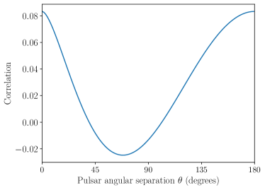
Figure 1: Left: the magnitude of the PTA response function $\Gamma^{(1)}_{ab}$ to kinematic dipole anisotropies, as defined in eq (2.24). We fix the velocity vector $\hat{v}$ along the the direction measured by the CMB ($\hat{v}$ and $-\hat{v}$ are denoted by red and yellow stars respectively). We plot the response as a function of the positions of a pair of pulsars, for simplicity oriented in the same direction. Right: the dipole response as a function of the angle between the pulsars, without including the $(\hat{v}\cdot\hat{x}_{a}+\hat{v}\cdot\hat{x}_{b})$ factor in eq (2.24).

We stress two important properties of the results reviewed so far

1. The quantities $\Gamma^{(1,2)}_{ab}$ vanish for pulsars with vectors orthogonal to the velocity: see eqs (2.24) and (2.25). Hence, the magnitude of kinematic anisotropies depend on the geometric configuration of the pulsar set: pulsars located along the direction of the velocity vector $\hat{v}$ are more sensitive to kinematic effects.

2. The effect of anisotropies depend on the frequency profile of the GW intensity: if $\bar{I}(f)$ has features in frequency which amplify the spectral tilts, anisotropy effects can get enhanced as they multiplied by combinations of $n_{I}$ and $\alpha_{I}$. In fact, the study of Doppler anisotropies provides additional tools for probing the frequency dependence of the GW intensity, besides more direct reconstruction techniques (see e.g. [81] and references therein).

The formulas presented in this section constitute the theoretical background we need next for analysing to what extent PTA experiments can probe kinematic anisotropies in the SGWB.

3 Kinematic anisotropies and present day PTA data

We are interested in measuring kinematic Doppler anisotropies in the SGWB with the present generation of PTA measurements, starting from the theoretical formulas discussed in section 2.

For the case of astrophysics backgrounds, the size of the intrinsic anisotropies is larger than the kinematic ones we are interested in. For cosmological SGWB, though, intrinsic anisotropies are usually small in amplitude, and kinematic effects provide the main contribution to anisotropies (see our discussion in section 1). GW experiments, if able to detect kinematic anisotropies, offer an independent tool to measure our motion relative to the cosmic source of GW, possibly helping to address the current anomaly in the measurements of the size of the relative velocity $\beta$ among frames reviewed in section 1. Additionally, they can provide independent tests for alternative theories of gravity [56, 54]. For this reason, it is worth exploring at what extent Doppler effects can be detected with PTA experiments.

In this section, we focus on current generation PTA experiments, which monitor a finite number of pulsars (around one hundred), placed in specific positions in the sky. We consider this kind of experimental set-up as ‘realistic’. So far, SGWB anisotropies have not been detected with PTA data: only upper limits on their size have been placed [51]. Using an approach based on the Fisher formalism, we develop tools for quantitatively searching for Doppler anisotropies, and for investigating to what extent realistic current-type PTA experiments should be improved towards this aim. In particular, we consider the current NANOGrav data set, (hereafter NG15) [1], and we then proceed demonstrating how including extra pulsars at specific positions in the sky can improve the sensitivity to Doppler effects. In fact, we are interested in developing the first of our comments at the end of section 2.

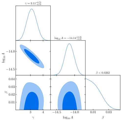
Figure 2: Parameter distributions and $95\%$ C.L limits for the SGWB amplitude $A$ ((A.8)), spectral index $\gamma$ (A.3) and dipole magnitude $\beta$. (See main text and Appendix A for the definition of these quantities.) The recovered amplitude and tilt are consistent with the NG15 results. We also obtain $\beta<0.026$ at $95\%$ C.L.

But before forecasting the capabilities of PTA experiments to measure kinematic effects by developing a dedicated Fisher formalism, we start by using the most recent NG15 data to extract what information they can provide on Doppler effects. Namely, we analyse for the first time the current NG15 dataset [1], searching for the presence of the kinematic dipole, fixing the dipole direction to the one measured by CMB experiments. The parameters that we vary are $\{\log_{10}A,\gamma,\beta\}$ and the red noise parameters (amplitude and spectral index) for each pulsar (see appendix A for our conventions on the quantities characterising the SGWB). We access the likelihood used by the NANOGrav collaboration through ENTERPRISE [82] and ENTERPRISE_EXTENSIONS [83]. The parameter space is explored using a Markov Chain Monte Carlo sampler [84, 85], through its interface with Cobaya [86]. Our results are plotted in Fig 2 using GetDist [87]. The parameter limits for the SGWB amplitude and spectral shape are consistent with those obtained in [1] and we set an upper limit $\beta<0.026$ at $95\%$ C.L, assuming a cosmological origin for the SGWB. Clearly, current data do not reach the per mil sensitivities on $\beta$, which are needed to set meaningful constraints on this quantity.

3.1 Extracting information from data

We now develop our own application of the Fisher formalism, tailored to extract information on Doppler effects from PTA results. We start with a general discussion on how to extract information on model parameters from data. We find it convenient to adopt the approach and notation from [36, 37]. We denote a given pulsar pair $(a,b)$ with the capital letter $A$: $(a,b)\to A$. The GW-induced time residual is

$$R_{A}^{\rm GW}\,=\,\frac{\gamma_{A}\cdot I}{(4\pi f)^{2}}\,=\,\frac{\Gamma_{A}\cdot\bar{I}}{(4\pi f)^{2}}\,.$$ (3.1)

The dot $\cdot$ here indicates that we are working with bandwidth-integrated quantities, centered at frequency $f$, that is:

$$\frac{\Gamma_{A}\cdot\bar{I}}{(4\pi f)^{2}}\,=\,\int_{f-\Delta f/2}^{f+\Delta f/2}d\tilde{f}\,\frac{\Gamma_{A}(\tilde{f})\bar{I}(\tilde{f})}{(4\pi\tilde{f})^{2}}\,,$$ (3.2)

where $\bar{I}(f)$ is the isotropic value of the frequency given in eq (2.4), and $\Gamma_{A}=\Gamma_{ab}$ is the overlap reduction function of eq (2.22). We include kinematic effects up to the quadrupole of order $\beta^{2}$. In the equalities of eq (3.1), we can use $\gamma_{A}$ or $\Gamma_{A}$, following the steps between eqs (2.7) and (2.10), and integrating over all directions for passing from one equality to the other. In fact, in the first equality of eq (3.1), the dot also includes integration over directions.

We approximate the likelihood as Gaussian in the timing residual cross-spectra [36]. We can then write

$$-2\ln\mathcal{L} = {\mathrm{const.}}+\sum_{f}\sum_{AB}\left(\hat{\mathcal{R}}_{A}-\frac{\gamma_{A}\cdot I}{(4\pi f)^{2}}\right)\,C^{-1}_{AB}\,\left(\hat{\mathcal{R}}_{B}-\frac{\gamma_{B}\cdot I}{(4\pi f)^{2}}\right)$$ (3.3)

$$= {\mathrm{const.}}+\sum_{f}\sum_{AB}\left(\hat{\mathcal{R}}_{A}-\frac{\Gamma_{A}\cdot\bar{I}}{(4\pi f)^{2}}\right)\,C^{-1}_{AB}\,\left(\hat{\mathcal{R}}_{B}-\frac{\Gamma_{B}\cdot\bar{I}}{(4\pi f)^{2}}\right)\,,$$ (3.4)

where $\hat{\mathcal{R}}$ indicate the measured cross-correlated timing residuals, and $C^{-1}$ is the inverse covariance matrix. In passing from line (3.3) to (3.4), we integrate over directions. As derived in [36], the covariance matrix of the timing residual band-powers is a combination of time-residual correlators $\mathcal{R}_{A}\,=\,\mathcal{R}_{ab}$ with the following structure

$$C_{AA^{\prime}} =\frac{1}{2T_{AA^{\prime}}\Delta f}(\mathcal{R}_{aa^{\prime}}\mathcal{R}_{bb^{\prime}}+\mathcal{R}_{ab^{\prime}}\mathcal{R}_{a^{\prime}b})\,,$$ (3.5)

with $T_{AA^{\prime}}$ the effective total time of observations of the four pulsars $(a\,b\,a^{\prime}\,b^{\prime})$, and we assume that the bandwidth $\Delta f$ satisfies $1/T\ll\Delta f\ll f$. Furthermore, in the weak signal limit

$$I\ll(4\pi f^{2}\sigma^{2})\,,$$ (3.6)

which we assume from now on, we have (recall the definition of ${\cal R}_{A}$ in eq (2.15))

$$\mathcal{R}_{A}\approx R_{A}^{N}\,=\,\sigma^{2}_{a}\,,$$ (3.7)

where $\sigma^{2}_{a}$ is the (band-integrated) variance of the noise in pulsar $a$. Thus, in this limit, the diagonal elements are much larger than the off-diagonal ones. Therefore, the covariance can be effectively approximated as diagonal in the pulsar pairs $A,A^{\prime}$ [36] (see also [88] for the same approximation in the context of interferometers, as well as our appendix B).

$$C_{AA^{\prime}}\approx\frac{R_{A}^{N}\,R_{A^{\prime}}^{N}}{2\,T_{AA^{\prime}}\Delta f}\delta_{AA^{\prime}}\,,$$ (3.8)

Its inverse is also diagonal

$$(C)^{-1}_{AA^{\prime}}=\frac{2\,T_{AA^{\prime}}\Delta f}{R_{A}^{N}\,R_{A^{\prime}}^{N}}\delta_{AA^{\prime}}\,.$$ (3.9)

This property renders our analysis particularly straightforward. Notice that, in this approximation, the covariance matrix depends only on noise parameters.

From the likelihood (3.4) we can determine the best-fit values of parameters, and their errors. We assume that the combinations $\Gamma\cdot\bar{I}$ appearing in the likelihood of eq (3.4) depend on a vector $\vec{\Theta}$, whose components correspond to the parameters we wish to determine. For example, the behaviour of the intensity $\bar{I}(f)$ as function of frequency. Or, the size of our velocity $\beta$ with respect to the SGWB rest frame. The best fit values for the parameters are found extremising the function $\ln{\cal L}$:

$$\frac{\partial\,{\ln{\cal L}}}{\partial\Theta_{i}}\,=\,0\,.$$ (3.10)

The errors on the determination of parameters are controlled by the Fisher matrix, defined as [89] (see also [90] for a pedagogical account)

$$\mathcal{F}_{ij}=\left\langle-\frac{\partial\ln\mathcal{L}}{\partial\Theta_{i}\partial\Theta_{j}}\right\rangle\,,$$ (3.11)

in terms of the expectation value of the second derivatives of $\ln{\cal L}$. The minimum error on the measurement of the parameters $\Theta_{i}$ is (no sum on repeated indexes):

$$\Delta\Theta_{i}=\sqrt{({\cal F}^{-1})_{ii}}\,,$$ (3.12)

giving us an estimate of a lower bound on the experimental errors to measure our signal parameters.

3.2 Best-fit values for the model parameters: an example

We already emphasised that the PTA response to Doppler anisotropies depend on the relative position of the monitored pulsars with respect to the direction of the velocity vector among frames, see section 2. We now discuss how to practically exploit this property. We focus in this section on the specific case of power law frequency profile in the SGWB intensity rest frame:

$$\bar{I}(f)\,=\,I_{0}\,\left({f}/{f_{\star}}\right)^{n_{I}}\,,$$ (3.13)

with $I_{0}$ a constant amplitude, $n_{I}$ the constant spectral tilt, and $f_{\star}$ a reference frequency. By extremising the log likelihood along the parameter models, see eq (3.4), we discuss how combinations of measurements allow us to determine the values of $I_{0}$ – the amplitude of GW intensity – and $\beta$ – the magnitude of the relative velocity among frames.

We vary $\ln{\cal L}$ of eq (3.4) along $\beta$, $I_{0}$, $n_{I}$, and we set the variations to zero. To simplify next formulas, after taking the variations we evaluate them on a frequency band around the reference frequency $f_{\star}$, hence $\bar{I}(f=f_{\star})\,\simeq\,I_{0}$. Calling the combination $\hat{I}_{0}=I_{0}/(4\pi f_{\star})^{2}$, we find three conditions, that can be expressed as:

$$0 = \left[\hat{I}_{0}-\frac{(\Gamma^{(1)}\hat{\cal R})}{(\Gamma^{(0)}\Gamma^{(1)})}\right]+$$ (3.14)

$$+\frac{\beta\,\hat{I}_{0}}{3(\Gamma^{(0)}\Gamma^{(1)})}\left[(1+n_{I})(\Gamma^{(0)}\Gamma^{(0)})+3(n_{I}-2)(\Gamma^{(0)}\Gamma^{(2)})+3(n_{I}-1)(\Gamma^{(1)}\Gamma^{(1)})\right]$$

$$-\frac{\beta}{3(\Gamma^{(0)}\Gamma^{(1)})}\left[(1+n_{I})(\Gamma^{(0)}\hat{\cal R})+3(n_{I}-2)(\Gamma^{(2)}\hat{\cal R})\right]\,,$$

$$0 = \left[\hat{I}_{0}-\frac{(\Gamma^{(0)}\hat{\cal R})}{(\Gamma^{(0)}\Gamma^{(0)})}\right]+\frac{\beta\,(n_{I}-1)}{(\Gamma^{(0)}\Gamma^{(0)})}\left[2\hat{I}_{0}(\Gamma^{(0)}\Gamma^{(1)})-(\Gamma^{(1)}\hat{\cal R})\right]\,,$$ (3.15)

$$0 = \left[\hat{I}_{0}-\frac{(\Gamma^{(1)}\hat{\cal R})}{(\Gamma^{(0)}\Gamma^{(1)})}\right]+$$ (3.16)

$$-\frac{\beta\,\hat{I}_{0}}{6(\Gamma^{(0)}\Gamma^{(1)})}\left\{9(\Gamma^{(0)}\Gamma^{(2)})+6(\Gamma^{(1)}\Gamma^{(1)})-2n_{I}\left[(\Gamma^{(0)}\Gamma^{(0)})+3(\Gamma^{(0)}\Gamma^{(2)})+3(\Gamma^{(1)}\Gamma^{(1)})\right]\right\}$$

$$+\frac{\beta}{6(\Gamma^{(0)}\Gamma^{(1)})}\left[3(3-2n_{I})(\Gamma^{(2)}\hat{\cal R})-2n_{I}(\Gamma^{(0)}\hat{\cal R})\right]\,.$$

In writing the previous expressions, we adopt the abbreviations

$$(\Gamma^{(0)}\hat{\cal R})\,\equiv\,\sum_{A}\Gamma^{(0)}_{A}\,\hat{\cal R}_{A}$$ (3.17)

and analog ones for the other round parenthesis. In the previous formulas, $\hat{\cal R}_{A}$ indicate PTA measurements, while the overlap functions $\Gamma^{(i)}_{A}$, for $i=0,1,2$, depend only on the geometrical configuration of the pulsar set. See their definitions in eqs (2.23)-(2.25).

Taking the difference between (3.14) and (3.16), simplifications occur. We find the following condition involving a linear combination of the GW intensity only

$$\hat{I}_{0}\,=\,\frac{2\left(\Gamma^{(0)}\cdot\hat{\cal R}\right)-3\left(\Gamma^{(2)}\cdot\hat{\cal R}\right)}{2\left(\Gamma^{(0)}\cdot\Gamma^{(0)}\right)-3\left(\Gamma^{(2)}\cdot\Gamma^{(0)}\right)}\,.$$ (3.18)

Plugging eq (3.18) in (3.15), we find the relation

$$(\Gamma^{(2)}\Gamma^{(0)})\,(\Gamma^{(0)}\hat{\cal R})-(\Gamma^{(2)}\Gamma^{(0)})\,(\Gamma^{(2)}\hat{\cal R})\,=$$

$$=\frac{(1-n_{I})\,\beta}{3}\left\{4(\Gamma^{(1)}\Gamma^{(0)})\,(\Gamma^{(0)}\hat{\cal R})+\left[3(\Gamma^{(0)}\Gamma^{(2)})-2(\Gamma^{(0)}\Gamma^{(0)})\right]\,(\Gamma^{(1)}\hat{\cal R})-6(\Gamma^{(0)}\Gamma^{(1)})\,(\Gamma^{(2)}\hat{\cal R})\right\}\,,$$

(3.19)

which provides information on the size of kinematic effects. Suppose to make a set of measurements. We build the combination in the left hand side of eq (3.19). This quantity is expected to be small but generally non zero: it is proportional to the parameter $\beta$ as dictated by the right hand side of this relation. Hence, eq (3.19) suggests a practical way to estimate the size of the small parameter $\beta$ by appropriately assembling PTA measurements. While the formulas discussed so far are evaluated at a frequency around the reference frequency $f_{\star}$, it is straightforward to generalize them to arbitrary frequencies, and take the sum over all frequency bins. Notice also that if the pulsar positions $\hat{x}_{a}$ are orthogonal to the frame velocity $\hat{v}$, then the functions $\Gamma^{(1,2)}_{A}$ vanish. In this case, the previous equality (3.19) is trivially satisfied, and provides no information.

We now turn to estimating the errors in the measurements using the Fisher matrix approach.

3.3 Fisher forecasts

The Fisher formalism, based on a manipulation of second derivatives of the log likelihood, allows one to make forecasts of the capabilities of a given experiment (current or future) to measure a given set of parameters. We now investigate how an expansion of current pulsar set of NANOGrav collaboration [91, 92, 93, 94] improves the prospects to detect Doppler anisotropies, if certain conditions are satisfied. See Fig 3 for a plot of NANOGrav pulsar positions in the sky, along as the direction of the velocity vector $\hat{v}$ as measured by CMB experiments [95].

In fact, currently the isotropic part of the SGWB is only detected with an $\text{SNR}\sim 5$ in the NG15 data set [1]. Given that the size of dipole anisotropy is at per mil level relative to the monopole, we do not expect the data to provide accurate information on kinematic anisotropies at this stage: this is indeed what we found in plot 2. However, the Fisher formalism allows us to quantify what gain in sensitivity is required, for the measurement of the kinematic dipole.

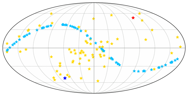
Figure 3: Representation of the sky position of the monitored NANOGrav pulsars (yellow), and the directions (positive and negative) of the velocity vector $\hat{v}$ among frames (red and dark blue stars), in galactic coordinates. Light blue stars indicate the position of pulsars in random positions orthogonal to the velocity vector.

We model our intensity signal as a power-law, as in eq (3.13), and we are interested in estimating the quantities $I_{0}$ and $\beta$ at first order in a Taylor expansion in $\beta$. Hence, we focus on the kinematic dipole. The Fisher matrix (3.11), when evaluated around the reference frequency $f_{\star}$ of eq (3.13), reads

$$\mathcal{F}_{ij}(f_{\star}) = \frac{1}{(4\pi f_{\star})^{4}}\sum_{A}\frac{2T_{A}\Delta f}{\left(R_{A}^{N}\right)^{2}}\,\begin{bmatrix}(\beta\kappa\,\Gamma^{(1)}_{A}+\Gamma^{(0)}_{A})^{2}&I_{0}\kappa\,\Gamma^{(1)}_{A}(\beta\kappa\Gamma^{(1)}_{A}+\Gamma^{(0)}_{A})\\ I_{0}\kappa\,\Gamma^{(1)}_{A}(\beta\kappa\Gamma^{(1)}_{A}+\Gamma^{(0)}_{A})&(I_{0}\kappa\,\Gamma^{(1)}_{A})^{2}\,,\end{bmatrix}$$

where the overlap functions $\Gamma^{(0,1)}_{A}$ are given in eqs (2.23), (2.25), and we denote with

$$\kappa=1-n_{I}\,$$ (3.21)

a convenient function of the intensity spectral index of eq (2.21). Eq (LABEL:fishrea) corresponds to the Fisher matrix for a given frequency $f$. The full Fisher matrix is obtained by then summing over the individual frequency bins

$$\mathcal{F}_{ij}=\sum_{f}\mathcal{F}_{ij}(f)\,.$$ (3.22)

For our fiducial model, we assume  the following parameter reference values for our plots (see (A.8)): $\log_{10}A=-14.6$ and $\gamma=13/3$.

$$I_{0} = 9.1\times 10^{-23}\,\hskip 14.22636pt,\hskip 14.22636pt\,f_{\star}\,=\,1/\mathrm{year},$$ (3.23)

$$\gamma=13/3\hskip 14.22636pt\Longleftrightarrow\hskip 14.22636ptn_{I}=-7/3,$$ (3.24)

and

$$\beta = 1.23\times 10^{-3}\hskip 14.22636pt,\hskip 14.22636pt\,\hat{v}\,=\,(l,b)=(264^{\circ},48^{\circ})$$ (3.25)

for the frame velocity amplitude and direction (the latter in galactic coordinates).

We can now discuss how our general approach allows to forecast how further developments in PTA experiments, for example monitoring more pulsars, can improve the sensitivity of kinematic anisotropies. As explained in section 2, the response of PTA experiments to kinematic anisotropies substantially depends on the position of the pulsars with respect to the velocity vector $\hat{v}$ among frames. We consider two cases including additional pulsars to the existing data set, see Fig 3. In the first case, we add 67 extra pulsars beside the 67 ones of NANOGrav collaboration, for simplicity each characterized by the same noise as an NG15 pulsar. The additional pulsars are all located in directions orthogonal to $\hat{v}$. Doubling the number of pulsars allows us to build many more pulsar pairs.

However, when pairing among the additional pulsars only, one finds that the sensitivity to Doppler anisotropies vanish, because the contributions $\Gamma^{(1,2)}_{ab}=0$ in eqs (2.24)-(2.25) since the pulsars are orthogonal to $\hat{v}$. As a consequence, although we somewhat gain in sensitivity, the error in the parameter $\beta$ is still large. See Fig 4, left panel. We then consider a second case, where we add 67 extra pulsars beside the 67 ones of NANOGrav collaboration, all located in a direction parallel to $\hat{v}$. We represent the result in Fig 4, right panel. In this case, formulas (2.24)-(2.25) indicate that the sensitivity to kinematic anisotropies should increase. In fact, we find that the error bars considerably reduce with respect to the first case discussed previously. Nevertheless, for both cases, working with order ${\cal O}(100)$ pulsars do not seem sufficient to achieve the desired per mil sensitivity on the value of $\beta$. In what comes next, we discuss futuristic PTA experiments that might be able to do so, by monitoring many more pulsars.

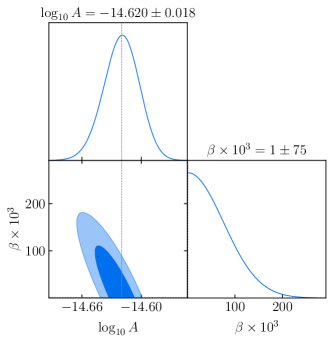
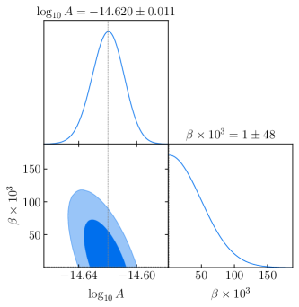
Figure 4: Results of our analysis when adding 67 additional pulsars to the NG15 data set, in directions orthogonal (left panel) and parallel (right panel) to the velocity vector $\hat{v}$, as explained in the main text.

4 Doppler anisotropies and future PTA data

After estimating the prospects for the present generation of PTA experiments to detect kinematic anisotropies in the SGWB, we now look towards the future, and we consider futuristic PTA experiments monitoring a very large number of pulsars. We assume to observe $N_{\rm psr}\gg{\cal O}(100)$ identical pulsars distributed isotropically across the sky, and observed for the same time period $T$. This is an optimistic condition, but in some approximation it might be achieved in the SKA era [55]. Given that the pulsars are assumed to be isotropically distributed, in this section we do not exploit their particular positions in the sky. Instead we investigate how a large number of pulsars improve the prospect to detect Doppler effects and consequently the magnitude and direction of the kinematic dipole. In first approximation, we can expect that the signal-to-noise ratio scales as the square root of the time of observation, times the square root of the number $N_{\rm pair}$ of pulsar pairs [31]. Since the latter scale as $N_{\rm pair}\,=\,N_{\rm psr}(N_{\rm psr}-1)/2\sim N_{\rm psr}^{2}/2$ for a large number of pulsars, increasing the quantity of pulsars considerably improves the prospects of detection.

For our forecasts we use the same approach of section 3.1. Additionally, in order to handle our formulas more easily, we use the techniques developed in [36]. We express the GW-induced two point correlators among time residuals as in eq (2.12): i.e., we do not integrate over directions, and we make use of the tensor $\gamma_{ab}$ of eq (2.8). The Fisher matrix, evaluated at frequency $f$, reads

$$\mathcal{F}_{ij}(f)=\frac{2T\Delta f}{(4\pi f\sigma)^{4}}N_{\rm pair}\times\frac{1}{N_{\rm pair}}\sum_{A}\gamma_{A}\cdot\frac{\partial I}{\partial\Theta_{i}}\gamma_{A}\cdot\frac{\partial I}{\partial\Theta_{j}}\,,\,$$ (4.1)

where $\sigma^{2}$ is the (common) noise variance. In writing (4.1), we vary over the parameters we wish to determine, as explained in section 3.1.

Using the results of [36], in the limit of large $N_{\rm psr}$ pulsars distributed isotropically across the sky, we can write

$$\frac{1}{N_{\rm pair}}\sum_{A}\gamma_{A}\cdot\frac{\partial I}{\partial\Theta_{i}}\gamma_{A}\cdot\frac{\partial I}{\partial\Theta_{j}}=\int\frac{d^{2}a}{4\pi}\frac{d^{2}b}{4\pi}\int\frac{d^{2}n}{4\pi}\frac{d^{2}n^{\prime}}{4\pi}\gamma_{ab}(\hat{n})\gamma_{ab}(\hat{n}^{\prime})\frac{\partial I(\hat{n})}{\partial\Theta_{i}}\frac{\partial I(\hat{n}^{\prime})}{\partial\Theta_{j}}\,,$$ (4.2)

where we replace the sum over pulsar pairs with an integral over the pulsar pair directions. Then, exchanging the order of the integrals, we can define a new function $\mathcal{F}_{\infty}$ as

$$\lim_{N_{\rm psr}\to\infty}\frac{1}{N_{\rm pair}}\sum_{ab}\gamma_{ab}(\hat{n})\,\gamma_{ab}(\hat{n}^{\prime}) =\int\frac{d^{2}a}{4\pi}\frac{d^{2}b}{4\pi}\gamma_{ab}(\hat{n})\,\gamma_{ab}(\hat{n}^{\prime})\,\equiv\,\mathcal{F}_{\infty}(\hat{n}\cdot\hat{n}^{\prime})\,.$$ (4.3)

Defining $\chi\equiv\hat{n}\cdot\hat{n}^{\prime}$, the function $\mathcal{F}_{\infty}(\chi)$ results in [36]

$$\mathcal{F}_{\infty}(\chi)=\frac{16}{9(1+\chi)^{2}}\times \Bigg{[}\left(\frac{1-\chi^{2}}{4}+2-\chi+3\frac{1-\chi}{1+\chi}\log\frac{1-\chi}{2}\right)^{2}$$

$$+\left(2-\chi+3\frac{1-\chi}{1+\chi}\log\frac{1-\chi}{2}\right)^{2}\Bigg{]}\,.$$ (4.4)

We emphasise that $\chi$ controls the angle between two GW directions. It is distinct from the angle $\zeta_{ab}$ used in eq (2.26).

At this point, given the isotropic distribution of the system, it is convenient to expand the quantities involved in spherical harmonics, and use their orthogonality properties. For the function $\mathcal{F}_{\infty}(\hat{n}\cdot\hat{n}^{\prime})$ we have

$$\mathcal{F}_{\infty}(\hat{n}\cdot\hat{n}^{\prime}) =4\pi\sum_{\ell m}\mathcal{F}_{\ell}\,Y_{\ell m}(\hat{n})Y_{\ell m}^{*}(\hat{n}^{\prime})$$ (4.5)

while for the anisotropic intensity – whose anisotropy is induced by kinematic effects as in eq (2.20) – we can write

$$I(f,\hat{n}) =\bar{I}(f)\,\left[1+\frac{4\pi}{3}\beta(n_{I}-1)\sum_{m}Y_{1m}(\hat{n})Y_{1m}^{*}(\hat{v})\right]\,.$$ (4.6)

We consider only dipolar anisotropies up to order $\beta$ (but notice that in the previous fornula $n_{I}$ can depend on frequency). The first three coefficients of $\mathcal{F}_{\infty}$ in eq (4.5) read $\mathcal{F}_{0}=4/27,\,\mathcal{F}_{1}=32\zeta(3)-\frac{346}{9}\approx 0.02,\,\mathcal{F}_{2}=\frac{46742}{135}-288\zeta(3)\approx 0.04$, with $\zeta(n)$ the Riemann zeta function.

Substituting expression (4.6) into our formula (4.1) for the Fisher matrix evaluated at a given frequency $f$, we find

$$\mathcal{F}_{ij}(f)=\frac{2T\Delta f}{(4\pi f\sigma)^{4}}N_{\rm pair}\times\left[\mathcal{F}_{0}\frac{\partial\bar{I}}{\partial\Theta_{i}}\frac{\partial\bar{I}}{\partial\Theta_{j}}+\frac{4\pi\mathcal{F}_{1}}{9}\sum_{m}\frac{\partial I_{1m}}{\partial\Theta_{i}}\frac{\partial I_{1m}^{*}}{\partial\Theta_{j}}\right]\,,$$ (4.7)

where

$$I_{1m}\equiv\bar{I}\,\beta\,\kappa\,Y_{1m}(\hat{v})\,,$$ (4.8)

(recall our definition of the parameter $\kappa=1-n_{I}$ in eq (3.21)). We vary along the intensity amplitude $\bar{I}$ – for simplicity we then evaluate the Fisher matrix at a reference frequency $f_{\star}$ –, alongwith the size of the frame velocity $\beta$, as well as along the dipole direction $\{\theta,\phi\}$ (which we later translate to galactic coordinates). We find

$$\mathcal{F}_{ij}(f_{\star})= \frac{2T\Delta f}{(4\pi f\sigma)^{4}}N_{pair}\times\begin{bmatrix}\mathcal{F}_{0}+\frac{\mathcal{F}_{1}\kappa^{2}\beta^{2}}{3}&\frac{\bar{I}\beta\mathcal{F}_{1}\kappa^{2}}{3}&0&0\\ \frac{\bar{I}\beta\mathcal{F}_{1}\kappa^{2}}{3}&\frac{\bar{I}^{2}{\mathcal{F}_{1}}\kappa^{2}}{3}&0&0\\ 0&0&\frac{\mathcal{F}_{1}\bar{I}^{2}\kappa^{2}\beta^{2}}{3}&0\\ 0&0&0&\frac{\mathcal{F}_{1}\bar{I}^{2}\kappa^{2}\beta^{2}\sin^{2}\theta}{3}\end{bmatrix}\,.$$ (4.9)

Once again, the full Fisher matrix will then be obtained by summing over the individual frequency bins.

4.1 Estimating the parameters in specific examples

We now apply the previous formulas to specific examples, in order to forecast in the idealized case of this section the accuracy in determining the model parameters, including the frequency dependence of the background.

4.1.1 Power-law scenario

Let us start with the example of a power-law frequency dependence of the SGWB in its rest frame, as the one of eq (3.13). Kinematic anisotropies, up to order $\beta$, lead to an anisotropic intensity of the form

$$I(f,\hat{n})=I_{0}(f/f_{\star})^{1-\kappa}(1+\beta\,\kappa\,\hat{n}\cdot\hat{v})\,,$$ (4.10)

with $\kappa=1-n_{I}$ as in eq (3.21), and $f_{\star}$ a reference frequency. Adding up the Fisher matrix over the frequency bins leads to

$$\mathcal{F}_{ij}=\sum_{f}\frac{2T\Delta f}{(4\pi f\sigma)^{4}}N_{pair}\left(\frac{f}{f_{\star}}\right)^{2-2\kappa}\times\begin{bmatrix}\mathcal{F}_{0}+\frac{\mathcal{F}_{1}\kappa^{2}\beta^{2}}{3}&\frac{I_{0}\beta\kappa^{2}\mathcal{F}_{1}}{3}&0&0\\ \frac{I_{0}\beta\kappa^{2}\mathcal{F}_{1}}{3}&\frac{I_{0}^{2}\kappa^{2}{\mathcal{F}_{1}}}{3}&0&0\\ 0&0&\frac{\mathcal{F}_{1}I_{0}^{2}\kappa^{2}\beta^{2}}{3}&0\\ 0&0&0&\frac{\mathcal{F}_{1}\,I_{0}^{2}\kappa^{2}\beta^{2}\sin^{2}\theta}{3}\end{bmatrix}\,.$$ (4.11)

We now focus on the component ${\cal F}_{\beta\beta}$, in order to Fisher estimate the error on the velocity amplitude (see section 3.3). We obtain

$$\mathcal{F}_{\beta\beta}=\sum_{f}\frac{2T\Delta f}{(4\pi f\sigma)^{4}}N_{pair}\left(\frac{f}{f_{\star}}\right)^{2-2\kappa}\frac{I_{0}^{2}\kappa^{2}\mathcal{F}_{1}}{3}=\text{SNR}_{\rm iso,\rm tot}^{2}\frac{\kappa^{2}\mathcal{F}_{1}}{3\mathcal{F}_{0}}\,,$$ (4.12)

where we identify the signal-to-noise ratio of the isotropic part as

$$\text{SNR}_{\rm iso,tot}^{2}=\sum_{f}\frac{2T\Delta f}{(4\pi f\sigma)^{4}}N_{pair}\left(\frac{f}{f_{\rm ref}}\right)^{2-2\kappa}I_{0}^{2}\mathcal{F}_{0}\,\,.$$ (4.13)

Therefore, the error in the measurement of $\beta$ becomes (at lowest order in $\beta$),

$$\Delta\beta=[F^{-1}]^{1/2}_{\beta\beta}\approx\left[\frac{3\mathcal{F}_{0}}{\text{SNR}_{\rm iso,\rm tot}^{2}\kappa^{2}\mathcal{F}_{1}}\right]^{1/2}\,.$$ (4.14)

As we know, CMB measurements give a value $\beta=1.2\times 10^{-3}$, which implies that for PTA experiments to measure this parameter with a precision of $\Delta\beta\sim 10^{-3}$ (in order for being competitive with other data sets) we must ensure at least

$$\text{SNR}_{\rm iso,tot}\sim 10^{3}\,.$$ (4.15)

Starting from these considerations, we can derive quantitative estimates for the error bars on the parameters involved, making some assumptions on the PTA measurements.

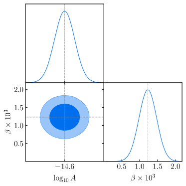
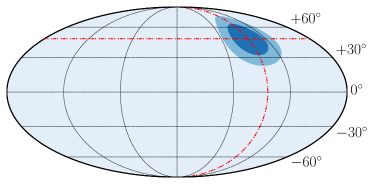
Figure 5: Fisher forecast for $\log_{10}A,\,\beta$ and the dipole direction parameters, as discussed in the main text around eq (4.16).

We take the time of observation $T_{\rm obs}=20\,\mathrm{years}$ and for the pulsar white noise parameters, we fix $T_{\rm cad}=\mathrm{year}/20$ as the cadence of the timing observations, $\Delta t_{\rm rms}=100\,\mathrm{ns}$ the rms error of the timing residuals [96]. For the red-noise parameters we take $A_{\rm RN}=3\times 10^{-16}$ and $\alpha_{\rm RN}=-2/3$. We then use Hasasia [97] to generate the noise curve. We perform a frequency binning, taking $\Delta f=1/T_{\rm obs}$ and $f\in[1/T_{\rm obs},20/T_{\rm obs}]$. For our fiducial parameters, we assume the same values as in section 3.3. Fixing this noise level, we choose the number of pulsars so as to obtain a roughly $15\%$ error in the determination of $\beta$. We find that for this we need 400 identical pulsars with the above noise properties to obtain such a precision. For this configuration, we plot the joint $68\%$ and $95\%$ confidence intervals for $\log_{10}A,\,\beta$ and the dipole direction parameters in figure 5. The parameter limits we obtain at $68\%$ level are

$$\log_{10}A =-14.6\pm 0.00004\,,$$ (4.16)

$$\beta =(1.23\pm 0.25)\times 10^{-3},$$ (4.17)

$$b =48\pm 10$$ (4.18)

$$l =264\pm 15\,.$$ (4.19)

where the two parameters $(l,b)$ indicate the dipole direction in galactic coordinates. Hence, we conclude that two decades of observations as well as the observation of 400 pulsars in this idealized case allows us to measure parameters controlling Doppler effects, with sufficient accuracy so that the results can be compared to other (CMB and LSS) data sets. In fact, since $N_{\rm pair}$ scales quadratically with $N_{\rm psr}$, the accuracy in the determination of the dipole parameters scales linearly with the number of pulsars in this idealised limit.

We also explored whether in this particular example we can use kinematic anisotropies to better constrain the slope of the spectrum $\kappa$, with respect to monopole measurements only. The answer is negative since for power law case information on the dipole anisotropy does not break any degeneracy between amplitude and slope of the spectrum. Instead, kinematic anisotropies are more informative with respect to the spectra slope for backgrounds more complex than a power law, as we are going to examine next.

4.1.2 Log-normal frequency spectrum

Our formalism is sufficiently flexible to allow us to go beyond the case of a power-law.

Figure 6: Fisher forecast of the dipole magnitude $\beta$ for log-normal spectrum of section 4.1.2. The parameter choices are shown in table 1, we obtain $\beta=(1.23\pm 0.5)\times 10^{-3}$ for $\Delta=1$ and $\beta=(1.23\pm 0.2)\times 10^{-3}$ for $\Delta=0.4$ (at $68\%$ C.L).

Let us consider a log-normal frequency profile in the SGWB rest frame, with a peaked frequency feature:

$$\bar{I}(f)=\frac{I_{0}}{\sqrt{2\pi}\Delta}\exp\left(-\frac{\ln^{2}(f/f_{0})}{2\Delta^{2}}\right)\,,$$ (4.20)

with $\Delta\ll 1$ corresponding to a sharply peaked narrow spectrum and $\Delta\gtrsim 1$ to a relatively broader spectrum.

The resulting Fisher forecasts, obtained following the same procedure of section 4.1.1, are plotted in figure 6, for the two cases $\Delta=0.4$ and $\Delta=1$.

To illustrate our point regarding the role of the frequency dependence, we focus only on the estimation of the dipole magnitude $\beta$. We consider two cases, namely a narrow and a broad spectrum with the parameter choices for both presented in table 1.

Parameter	Narrow	Broad
$\log_{10}I_{0}$	$-19.8$	-20.1
$f_{0}$	$0.2/\mathrm{year}$	$0.2/\mathrm{year}$
$\Delta$	$0.4$	$1$

Table 1: Parameter values for the narrow and broad log-normal power spectra.

The parameters are chosen in a manner such that the dipole can be measured with sufficient precision and such that the isotropic SNR for both cases is the same. We learn that sharper features in the frequency spectrum enhance kinematic effects, making them easier to detect in the $\Delta=0.4$ case compared to the $\Delta=1$ case. This is a particular example among many showing how the possibly rich frequency dependence of the GW spectrum can affect the detection of Doppler anisotropies.

5 Conclusions

The recent detection of a stochastic gravitational wave background by PTA collaborations represents a significant milestone in the field of GW astronomy. Given that the origin of this background is currently unknown, it is the task of theorists to identify signatures that could be used to discriminate between astrophysical and cosmological origin of the signal. In the near future, the IPTA DR3 release is likely to lead to more precise measurements of the amplitude and spectral shape and may provide hints to origin of the SGWB [5]. Another key signature is the anisotropy of the SGWB intensity, with astrophysical models predicting a much larger level of anisotropy compared to cosmological ones. Thus, future observation of anisotropies may decisively tilt the scales in favour of a cosmological or astrophysical original of the PTA signal.

Promisingly, recent forecasts of the detectability of astrophysical anisotropies suggest that a significant fraction of the predicted level of anisotropy may be detected in the current or near future data [51]. Although the prospects for detecting the intrinsic anisotropy of cosmological backgrounds are currently quite dire, this is not the case for the much larger kinematic dipole anisotropy which is generated due to our motion w.r.t the SGWB rest frame. Using the NG15 dataset, we are able to place an upper limit $\beta<0.026$ at $95\%$ C.L. on the magnitude of this dipole, assuming a cosmological origin for the signal and the dipole direction to be the same as inferred from the CMB. We also show that the kinematic dipole will be well within the reach of an SKA-like experiment, due to its lower noise levels and the significantly more pulsars it is expected to observe. For such an experiment, we demonstrate that measuring the dipole magnitude at a level $\Delta\beta/\beta\simeq 0.1$ and the direction $\Delta(l,b)\simeq 10^{\circ}$ is definitely a realistic target. We also highlight how the positions of the pulsars observed as well as the spectral shape of the SGWB affects the sensitivity to the kinematic dipole.

The increased sensitivity of SKA will allow for measurements of the dipole magnitude and direction at a level precise enough to test whether the rest frames of the CMB and cosmological SGWB coincide. While one would naturally expect this to be the case, the emergence of the recent CMB-LSS dipole tension underscores the importance of verifying this assumption experimentally. In this way, observation of the the SGWB kinematic dipole could enable us to not only pinpoint the origin of the PTA signal, but also serve as an independent test of the cosmological principle. Last, but not least, Doppler anisotropies can also provide independent tests of modifications of Einstein gravity. The search for their presence with PTA experiments is definitely worth pursuing.

Acknowledgments

We are partially funded by the STFC grants ST/T000813/1 and ST/X000648/1. We also acknowledge the support of the Supercomputing Wales project, which is part-funded by the European Regional Development Fund (ERDF) via Welsh Government. For the purpose of open access, the authors have applied a Creative Commons Attribution licence to any Author Accepted Manuscript version arising.

Appendix A Conventions on the SGWB parameters

The spectral energy density parameter $\Omega_{\rm GW}$ is related to the intensity $I$ through

$$\Omega_{\rm GW}=\frac{4\pi^{2}f^{3}}{3H_{0}^{2}}I\,.$$ (A.1)

Besides the GW energy density, another important quantity is the characteristic strain $h_{c}$, which we parametrise as a power law

$$h_{c}(f)\equiv\sqrt{2fI(f)}=A\left(\frac{f}{f_{\rm ref}}\right)^{\alpha}\,.$$ (A.2)

Note that for a background of supermassive black hole binaries, the expected parameters for the characteristic strain are $\alpha=-2/3$ and $A\approx 10^{-15}$. PTA collaborations typically report their results in terms of the parameters $A,\gamma$ where

$$\gamma\equiv 3-2\alpha.$$ (A.3)

The NG15 results for the amplitude $A$, when fixing $\alpha=-2/3$ and taking a reference frequency of $f_{\rm ref}=1/\mathrm{year}$ are [1]

$$A=2.4^{+0.7}_{-0.6}\times 10^{-15}\,(\text{at }90\%\text{ C.L.})\,.$$ (A.4)

For such a power law characteristic strain model, the spectral energy density can be expressed as

$$\Omega_{\rm GW}(f)=\frac{2\pi^{2}f^{2}}{3H_{0}^{2}}A^{2}\left(\frac{f}{f_{\rm ref}}\right)^{2\alpha}=\Omega_{\mathrm{GW},0}\left(\frac{f}{f_{\rm ref}}\right)^{n_{\Omega}}\,,$$ (A.5)

where

$$\Omega_{\mathrm{GW},0}\equiv\frac{2\pi^{2}}{3H_{0}^{2}}f_{\rm ref}^{2}A^{2},\quad n_{\Omega}\equiv 2\alpha+2\,.$$ (A.6)

Similarly, for the intensity we have

$$I(f)=\frac{A^{2}}{2f}\left(\frac{f}{f_{\rm ref}}\right)^{2\alpha}=I_{0}\left(\frac{f}{f_{\rm ref}}\right)^{n_{I}}\,,$$ (A.7)

where

$$I_{0}\equiv\frac{A^{2}}{2f_{\rm ref}},\quad n_{I}\equiv 2\alpha-1\,.$$ (A.8)

Plugging in the value of $A$ measured by NANOGrav (A.4), we have

$$\Omega_{\mathrm{GW},0}\approx 8.1\times 10^{-9},\quad I_{0}\approx 9.1\times 10^{-23}[s]\,.$$ (A.9)

If instead, we take as our reference frequency $f_{\rm ref}=0.1/\mathrm{year}$ we obtain,

$$\Omega_{\mathrm{GW},0}\approx 5.6\times 10^{-10},\quad I_{0}\approx 6.3\times 10^{-21}[s]\,.$$ (A.10)

Appendix B Covariance matrix in the weak signal limit

We now provide arguments to explain why the covariance matrix in our likelihood is effectively diagonal in the weak signal limit – see the discussion after eq (3.5). Our arguments are not specific to PTA experiments, but they are also applicable to ground based interferometers. Let $d_{I}$ denote the data recorded by a given detector and $N_{I}$ denote its noise PSD. The data is the sum of the signal and noise, i.e.

$$d_{I}=s_{I}+n_{I},\,\quad\langle{d_{I}}\rangle=\langle{s_{I}}\rangle,\quad\langle{n_{I}}\rangle=0\,.$$ (B.1)

We write the likelihood as

$$-2\ln\mathcal{L}=\sum_{IJ}(\hat{d}_{I}-s_{I})\,C^{-1}_{IJ}\,(\hat{d}_{J}-s_{J})^{T}\,,$$ (B.2)

where the covariance $C_{IJ}$ is given by

$$C_{IJ}=\langle{d_{I}d_{J}}\rangle-\langle{d_{I}}\rangle\langle{d_{J}}\rangle\,.$$ (B.3)

Suppose for simplicity we have only two detectors, so that $C_{IJ}$ is a $2\times 2$ matrix. Then assuming the noise is uncorrelated across detectors, and that the detectors have the same noise variance, we find

$$C_{IJ}=\begin{pmatrix}N+\langle{s_{I}^{2}}\rangle&\langle{s_{I}s_{J}}\rangle\\ \langle{s_{I}s_{J}}\rangle&N+\langle{s_{J}^{2}}\rangle\end{pmatrix}\,.$$ (B.4)

For ease of notation, we assume $\langle{s_{I}}\rangle=\langle{s_{J}}\rangle=s$ and $\langle{s_{I}^{2}}\rangle=\langle{s_{J}^{2}}\rangle=\langle{s_{I}s_{J}}\rangle=\langle{s^{2}}\rangle$. Evaluating the full likelihood for the signal with the above covariance matrix gives

$$-2\ln\mathcal{L}=\frac{2(\hat{d}-s)^{2}}{N+2s^{2}}\approx\frac{2(\hat{d}-s)^{2}}{N}$$ (B.5)

in the weak signal limit $s^{2}\ll N$. Thus, in this limit we approximate the covariance matrix as effectively diagonal,

$$C_{IJ}\approx\begin{pmatrix}N&0\\ 0&N\end{pmatrix}\,,$$ (B.6)

as claimed.

Appendix C Full Fisher matrix with contributions up to order $\beta^{2}$

For convenience, in this appendix we express the intensity as

$$I(f,\hat{n})=I_{0}H(f)\left[1+m_{I}(f)\beta^{2}+\xi d_{I}(f)\beta+\frac{1}{2}(3\xi^{2}-1)q_{I}(f)\beta^{2}\right]\,,$$ (C.1)

with $\xi=\hat{n}\cdot\hat{v}$ and

$$m_{I}(f) =\frac{1}{6}(-1+n_{I}^{2}+\kappa_{I})\,,$$ (C.2)

$$d_{I}(f) =(1-n_{I})\,,$$ (C.3)

$$q_{I}(f) =\frac{1}{3}[\kappa_{I}+(n_{I}-2)(n_{I}-1)]\,.$$ (C.4)

We consider two cases. A realistic case with finite number of pulsars, as in section 3, and an idealised case with a very large number of pulsars distributed isotropically in the sky, as in section 4.

C.1 Realistic case

The full likelihood with quadrupole and monopole correction added is

$$-2\ln\mathcal{L}=\mathrm{const.}+\sum_{f}\sum_{pq}\left(\hat{\mathcal{R}}_{pq}-\frac{I_{0}H(f)(\Gamma_{pq}^{(0)}(1+\beta^{2}m_{I})+\beta(1-n_{I})\Gamma_{pq}^{(1)}+\beta^{2}q_{I}\Gamma^{(2)}_{pq})}{(4\pi f)^{2}}\right)^{2}\,N^{-1}_{pq}\,,$$ (C.5)

with

$$\Gamma^{(2)}_{pq} \equiv\frac{1}{2}\int\frac{d^{2}\hat{n}}{4\pi}\,{\gamma_{pq}(\hat{n})}(3\xi^{2}-1)\,.$$ (C.6)

We obtain the following Fisher matrix for $\{I_{0},\beta\}$,

$$\mathcal{F}_{ij,f}=\frac{1}{(4\pi f)^{4}}\sum_{pq}\frac{2T_{pq}\Delta f}{\sigma_{p}^{2}\sigma_{q}^{2}}H^{2}(f)\,\begin{bmatrix}a_{I_{0}I_{0}}&a_{I_{0}\beta}\\ a_{\beta I_{0}}&a_{\beta\beta}\,,\end{bmatrix}$$ (C.7)

with

$$a_{I_{0}I_{0}}= \left(\beta(\kappa\Gamma^{(1)}_{pq}+q\beta\Gamma^{(2)}_{pq})+\Gamma^{(0)}_{pq}\left(\beta^{2}m+1\right)\right)^{2}\approx(\Gamma^{(0)}_{pq})^{2}+\mathcal{O}(\beta)$$ (C.8)

$$a_{I_{0}\beta}= \,a_{\beta I_{0}}=I_{0}\left(\beta(\kappa\Gamma^{(1)}_{pq}+q\beta\Gamma^{(2)}_{pq})+\Gamma^{(0)}_{pq}\left(\beta^{2}m+1\right)\right)\left(\kappa\Gamma^{(1)}_{pq}+2\beta\Gamma_{0}m+2\beta\Gamma^{(2)}_{pq}q\right)$$ (C.9)

$$\approx \,I_{0}\kappa\Gamma^{(0)}\Gamma^{(1)}_{pq}+\mathcal{O}(\beta)$$ (C.10)

$$a_{\beta\beta}= I_{0}^{2}\left(\kappa\Gamma^{(1)}_{pq}+\beta(m\Gamma^{(0)}_{pq}+q\Gamma^{(2)}_{pq})\right)^{2}\approx(I_{0}\kappa\Gamma^{(1)}_{pq})^{2}+\mathcal{O}(\beta)\,.$$ (C.11)

Thus, in the limit $\beta\ll 1$, the contributions of the quadrupole and the monopole correction are subdominant compared to the dipole. However, in the realistic case, the Fisher matrix also depends on the exact configuration of pulsars. Although both the dipole and quadrupole response vanish for pulsars orthogonal to the velocity, the exact dependence is slightly different and it is indeed possible that for certain configurations of pulsars the quadrupole response is as or more important than the dipole.

C.2 Idealised case

Proceeding similarly to section 4 we obtain

$$\mathcal{F}_{ij,f} =\frac{2T\Delta f}{(4\pi f\sigma)^{4}}N_{pair}H^{2}(f)\times\begin{bmatrix}a_{I_{0}I_{0}}&a_{I_{0}\beta}&0&0\\ a_{\beta I_{0}}&a_{\beta\beta}&0&0\\ 0&0&a_{\theta\theta}&0\\ 0&0&0&a_{\phi\phi}\end{bmatrix}\,,$$ (C.12)

where

$$a_{I_{0}I_{0}} =\mathcal{F}_{0}\left(m_{I}\beta^{2}+1\right)^{2}+\frac{1}{3}\beta^{2}\mathcal{F}_{1}(n_{I}-1)^{2}+\frac{1}{5}\mathcal{F}_{2}q_{I}^{2}\beta^{4}\approx\mathcal{F}_{0}+\mathcal{O}(\beta^{2})$$ (C.13)

$$a_{\beta\beta} =\frac{1}{15}I_{0}^{2}\left({12\beta^{2}}\left(5\mathcal{F}_{0}m_{I}^{2}+\mathcal{F}_{2}q_{I}^{2}\right)+5\mathcal{F}_{1}(n_{I}-1)^{2}\right)\approx\frac{\mathcal{F}_{1}I_{0}^{2}(n_{I}-1)^{2}}{3}+\mathcal{O}(\beta^{2})$$ (C.14)

$$a_{I_{0}\beta} =a_{\beta I_{0}}=\frac{1}{15}\beta I_{0}\left(30\mathcal{F}_{0}{m_{I}}\left(m_{I}\beta^{2}+1\right)+5\mathcal{F}_{1}(n_{I}-1)^{2}+6\mathcal{F}_{2}{q_{I}^{2}}{\beta^{2}}\right)$$ (C.15)

$$\approx\beta I_{0}\left({2\mathcal{F}_{0}m_{I}}+\frac{\mathcal{F}_{1}(n_{I}-1)^{2}}{3}\right)+\mathcal{O}(\beta^{3})\,,$$ (C.16)

$$a_{\theta\theta} =\frac{1}{15}\beta^{2}I_{0}^{2}\left(5\mathcal{F}_{1}(n_{I}-1)^{2}+9\mathcal{F}_{2}{q_{I}^{2}}{\beta^{2}}\right)\approx\frac{\mathcal{F}_{1}I_{0}^{2}(n_{I}-1)^{2}}{3}\beta^{2}+\mathcal{O}(\beta^{4})$$ (C.17)

$$a_{\phi\phi} =\frac{1}{15}\beta^{2}I_{0}^{2}\sin^{2}\theta\left(5\mathcal{F}_{1}(n_{I}-1)^{2}+9\mathcal{F}_{2}{q_{I}^{2}}{\beta^{2}}\right)\approx\frac{\mathcal{F}_{1}I_{0}^{2}(n_{I}-1)^{2}}{3}\beta^{2}\sin^{2}\theta+\mathcal{O}(\beta^{4})\,,$$ (C.18)

Incorporating all higher multipoles ($\ell\geq 1$) of the anisotropy induced by kinematic effects, i.e.

$$I(\hat{n})=\sum_{\ell\geq 1}I_{\ell}\,\mathcal{P}_{\ell}(\hat{n}\cdot\hat{v})=4\pi\sum_{\ell\geq 2}\sum_{m=-\ell}^{\ell}\frac{I_{\ell}}{(2\ell+1)}\,Y_{\ell m}(\hat{n})Y_{\ell m}^{*}(\hat{v})\,,$$ (C.19)

we obtain a Fisher matrix of the form

$$F_{ij}=\frac{2T\Delta f}{(4\pi f\sigma)^{4}}N_{pair}\times\left[\mathcal{F}_{0}\frac{\partial I_{0}(1+m_{I}\beta^{2})}{\partial\Theta_{i}}\frac{\partial I_{0}(1+m_{I}\beta^{2})}{\partial\Theta_{j}}+4\pi\sum_{\ell\geq 1}\sum_{m=-\ell}^{\ell}\frac{\mathcal{F}_{\ell}}{(2\ell+1)^{2}}\frac{\partial I_{\ell m}}{\partial\Theta_{i}}\frac{\partial I_{\ell m}^{*}}{\partial\Theta_{j}}\right]\,,$$ (C.20)

where we defined $I_{\ell m}\equiv I_{\ell}\,Y_{\ell m}(\hat{v})$.

References

- [1] NANOGrav Collaboration, G. Agazie et al., “The NANOGrav 15 yr Data Set: Evidence for a Gravitational-wave Background,” Astrophys. J. Lett. 951 no. 1, (2023) L8, arXiv:2306.16213 [astro-ph.HE].
- [2] D. J. Reardon et al., “Search for an Isotropic Gravitational-wave Background with the Parkes Pulsar Timing Array,” Astrophys. J. Lett. 951 no. 1, (2023) L6, arXiv:2306.16215 [astro-ph.HE].
- [3] H. Xu et al., “Searching for the Nano-Hertz Stochastic Gravitational Wave Background with the Chinese Pulsar Timing Array Data Release I,” Res. Astron. Astrophys. 23 no. 7, (2023) 075024, arXiv:2306.16216 [astro-ph.HE].
- [4] EPTA, InPTA: Collaboration, J. Antoniadis et al., “The second data release from the European Pulsar Timing Array - III. Search for gravitational wave signals,” Astron. Astrophys. 678 (6, 2023) A50, arXiv:2306.16214 [astro-ph.HE].
- [5] International Pulsar Timing Array Collaboration, G. Agazie et al., “Comparing recent PTA results on the nanohertz stochastic gravitational wave background,” arXiv:2309.00693 [astro-ph.HE].
- [6] A. Sesana, A. Vecchio, and C. N. Colacino, “The stochastic gravitational-wave background from massive black hole binary systems: implications for observations with Pulsar Timing Arrays,” Mon. Not. Roy. Astron. Soc. 390 (2008) 192, arXiv:0804.4476 [astro-ph].
- [7] S. Burke-Spolaor et al., “The Astrophysics of Nanohertz Gravitational Waves,” Astron. Astrophys. Rev. 27 no. 1, (2019) 5, arXiv:1811.08826 [astro-ph.HE].
- [8] C. Caprini and D. G. Figueroa, “Cosmological Backgrounds of Gravitational Waves,” Class. Quant. Grav. 35 no. 16, (Aug., 2018) 163001, arXiv:1801.04268 [astro-ph.CO]. https://iopscience.iop.org/article/10.1088/1361-6382/aac608.
- [9] N. J. Cornish and A. Sesana, “Pulsar Timing Array Analysis for Black Hole Backgrounds,” Class. Quant. Grav. 30 (2013) 224005, arXiv:1305.0326 [gr-qc].
- [10] C. M. Mingarelli, T. Sidery, I. Mandel, and A. Vecchio, “Characterizing gravitational wave stochastic background anisotropy with pulsar timing arrays,” Phys. Rev. D 88 no. 6, (2013) 062005, arXiv:1306.5394 [astro-ph.HE].
- [11] S. R. Taylor and J. R. Gair, “Searching For Anisotropic Gravitational-wave Backgrounds Using Pulsar Timing Arrays,” Phys. Rev. D 88 (2013) 084001, arXiv:1306.5395 [gr-qc].
- [12] C. M. F. Mingarelli, T. J. W. Lazio, A. Sesana, J. E. Greene, J. A. Ellis, C.-P. Ma, S. Croft, S. Burke-Spolaor, and S. R. Taylor, “The local nanohertz gravitational-wave landscape from supermassive black hole binaries,” Nature Astronomy 1 (Nov., 2017) 886–892, arXiv:1708.03491 [astro-ph.GA].
- [13] N. J. Cornish and L. Sampson, “Towards Robust Gravitational Wave Detection with Pulsar Timing Arrays,” Phys. Rev. D 93 no. 10, (2016) 104047, arXiv:1512.06829 [gr-qc].
- [14] S. R. Taylor, R. van Haasteren, and A. Sesana, “From Bright Binaries To Bumpy Backgrounds: Mapping Realistic Gravitational Wave Skies With Pulsar-Timing Arrays,” Phys. Rev. D 102 no. 8, (2020) 084039, arXiv:2006.04810 [astro-ph.IM].
- [15] B. Bécsy, N. J. Cornish, and L. Z. Kelley, “Exploring Realistic Nanohertz Gravitational-wave Backgrounds,” Astrophys. J. 941 no. 2, (2022) 119, arXiv:2207.01607 [astro-ph.HE].
- [16] B. Allen, “Variance of the Hellings-Downs correlation,” Phys. Rev. D 107 no. 4, (2023) 043018, arXiv:2205.05637 [gr-qc].
- [17] G. Sato-Polito and M. Kamionkowski, “Pulsar-timing measurement of the circular polarization of the stochastic gravitational-wave background,” Phys. Rev. D 106 no. 2, (2022) 023004, arXiv:2111.05867 [astro-ph.CO].
- [18] G. Sato-Polito and M. Kamionkowski, “Exploring the spectrum of stochastic gravitational-wave anisotropies with pulsar timing arrays,” arXiv:2305.05690 [astro-ph.CO].
- [19] V. Alba and J. Maldacena, “Primordial gravity wave background anisotropies,” JHEP 03 (2016) 115, arXiv:1512.01531 [hep-th].
- [20] C. R. Contaldi, “Anisotropies of Gravitational Wave Backgrounds: A Line Of Sight Approach,” Phys. Lett. B 771 (2017) 9–12, arXiv:1609.08168 [astro-ph.CO].
- [21] M. Geller, A. Hook, R. Sundrum, and Y. Tsai, “Primordial Anisotropies in the Gravitational Wave Background from Cosmological Phase Transitions,” Phys. Rev. Lett. 121 no. 20, (2018) 201303, arXiv:1803.10780 [hep-ph].
- [22] N. Bartolo, D. Bertacca, S. Matarrese, M. Peloso, A. Ricciardone, A. Riotto, and G. Tasinato, “Anisotropies and non-Gaussianity of the Cosmological Gravitational Wave Background,” Phys. Rev. D 100 no. 12, (2019) 121501, arXiv:1908.00527 [astro-ph.CO].
- [23] N. Bartolo, D. Bertacca, V. De Luca, G. Franciolini, S. Matarrese, M. Peloso, A. Ricciardone, A. Riotto, and G. Tasinato, “Gravitational wave anisotropies from primordial black holes,” JCAP 02 (2020) 028, arXiv:1909.12619 [astro-ph.CO].
- [24] N. Bartolo, D. Bertacca, S. Matarrese, M. Peloso, A. Ricciardone, A. Riotto, and G. Tasinato, “Characterizing the cosmological gravitational wave background: Anisotropies and non-Gaussianity,” Phys. Rev. D 102 no. 2, (2020) 023527, arXiv:1912.09433 [astro-ph.CO].
- [25] LISA Cosmology Working Group Collaboration, N. Bartolo et al., “Probing anisotropies of the Stochastic Gravitational Wave Background with LISA,” JCAP 11 (2022) 009, arXiv:2201.08782 [astro-ph.CO].
- [26] G. F. Smoot, M. V. Gorenstein, and R. A. Muller, “Detection of Anisotropy in the Cosmic Black Body Radiation,” Phys. Rev. Lett. 39 (1977) 898.
- [27] A. Kogut et al., “Dipole anisotropy in the COBE DMR first year sky maps,” Astrophys. J. 419 (1993) 1, arXiv:astro-ph/9312056.
- [28] WMAP Collaboration, C. L. Bennett et al., “First year Wilkinson Microwave Anisotropy Probe (WMAP) observations: Preliminary maps and basic results,” Astrophys. J. Suppl. 148 (2003) 1–27, arXiv:astro-ph/0302207.
- [29] WMAP Collaboration, G. Hinshaw et al., “Five-Year Wilkinson Microwave Anisotropy Probe (WMAP) Observations: Data Processing, Sky Maps, and Basic Results,” Astrophys. J. Suppl. 180 (2009) 225–245, arXiv:0803.0732 [astro-ph].
- [30] Planck Collaboration, N. Aghanim et al., “Planck 2013 results. XXVII. Doppler boosting of the CMB: Eppur si muove,” Astron. Astrophys. 571 (2014) A27, arXiv:1303.5087 [astro-ph.CO].
- [31] M. Anholm, S. Ballmer, J. D. E. Creighton, L. R. Price, and X. Siemens, “Optimal strategies for gravitational wave stochastic background searches in pulsar timing data,” Phys. Rev. D 79 (2009) 084030, arXiv:0809.0701 [gr-qc].
- [32] J. Gair, J. D. Romano, S. Taylor, and C. M. F. Mingarelli, “Mapping gravitational-wave backgrounds using methods from CMB analysis: Application to pulsar timing arrays,” Phys. Rev. D 90 no. 8, (2014) 082001, arXiv:1406.4664 [gr-qc].
- [33] N. J. Cornish and R. van Haasteren, “Mapping the nano-Hertz gravitational wave sky,” arXiv:1406.4511 [gr-qc].
- [34] C. M. F. Mingarelli, T. J. W. Lazio, A. Sesana, J. E. Greene, J. A. Ellis, C.-P. Ma, S. Croft, S. Burke-Spolaor, and S. R. Taylor, “The Local Nanohertz Gravitational-Wave Landscape From Supermassive Black Hole Binaries,” Nature Astron. 1 no. 12, (2017) 886–892, arXiv:1708.03491 [astro-ph.GA].
- [35] S. C. Hotinli, M. Kamionkowski, and A. H. Jaffe, “The search for anisotropy in the gravitational-wave background with pulsar-timing arrays,” Open J. Astrophys. 2 no. 1, (2019) 8, arXiv:1904.05348 [astro-ph.CO].
- [36] Y. Ali-Haïmoud, T. L. Smith, and C. M. F. Mingarelli, “Fisher formalism for anisotropic gravitational-wave background searches with pulsar timing arrays,” Phys. Rev. D 102 no. 12, (2020) 122005, arXiv:2006.14570 [gr-qc].
- [37] Y. Ali-Haïmoud, T. L. Smith, and C. M. F. Mingarelli, “Insights into searches for anisotropies in the nanohertz gravitational-wave background,” Phys. Rev. D 103 no. 4, (2021) 042009, arXiv:2010.13958 [gr-qc].
- [38] N. Pol, S. R. Taylor, and J. D. Romano, “Forecasting Pulsar Timing Array Sensitivity to Anisotropy in the Stochastic Gravitational Wave Background,” Astrophys. J. 940 no. 2, (2022) 173, arXiv:2206.09936 [astro-ph.HE].
- [39] B. Allen and A. C. Ottewill, “Detection of anisotropies in the gravitational wave stochastic background,” Phys. Rev. D 56 (1997) 545–563, arXiv:gr-qc/9607068 [gr-qc].
- [40] S. W. Ballmer, “A Radiometer for stochastic gravitational waves,” Class. Quant. Grav. 23 (2006) S179–S186, arXiv:gr-qc/0510096.
- [41] E. Thrane, S. Ballmer, J. D. Romano, S. Mitra, D. Talukder, S. Bose, and V. Mandic, “Probing the anisotropies of a stochastic gravitational-wave background using a network of ground-based laser interferometers,” Phys. Rev. D 80 (2009) 122002, arXiv:0910.0858 [astro-ph.IM].
- [42] A. I. Renzini and C. R. Contaldi, “Mapping Incoherent Gravitational Wave Backgrounds,” Mon. Not. Roy. Astron. Soc. 481 no. 4, (2018) 4650–4661, arXiv:1806.11360 [astro-ph.IM].
- [43] E. Payne, S. Banagiri, P. Lasky, and E. Thrane, “Searching for anisotropy in the distribution of binary black hole mergers,” Phys. Rev. D 102 no. 10, (2020) 102004, arXiv:2006.11957 [astro-ph.CO].
- [44] N. J. Cornish, “Mapping the gravitational wave background,” Class. Quant. Grav. 18 (2001) 4277–4292, arXiv:astro-ph/0105374.
- [45] J. Baker et al., “High angular resolution gravitational wave astronomy,” Exper. Astron. 51 no. 3, (8, 2021) 1441–1470, arXiv:1908.11410 [astro-ph.HE].
- [46] S. Banagiri, A. Criswell, T. Kuan, V. Mandic, J. D. Romano, and S. R. Taylor, “Mapping the gravitational-wave sky with LISA: a Bayesian spherical harmonic approach,” Mon. Not. Roy. Astron. Soc. 507 no. 4, (2021) 5451–5462, arXiv:2103.00826 [astro-ph.IM].
- [47] C. R. Contaldi, M. Pieroni, A. I. Renzini, G. Cusin, N. Karnesis, M. Peloso, A. Ricciardone, and G. Tasinato, “Maximum likelihood map-making with the Laser Interferometer Space Antenna,” Phys. Rev. D 102 no. 4, (2020) 043502, arXiv:2006.03313 [astro-ph.CO].
- [48] G. Mentasti and M. Peloso, “ET sensitivity to the anisotropic Stochastic Gravitational Wave Background,” JCAP 03 (2021) 080, arXiv:2010.00486 [astro-ph.CO].
- [49] G. Mentasti, C. R. Contaldi, and M. Peloso, “Intrinsic Limits on the Detection of the Anisotropies of the Stochastic Gravitational Wave Background,” Phys. Rev. Lett. 131 no. 22, (2023) 221403, arXiv:2301.08074 [gr-qc].
- [50] S. R. Taylor et al., “Limits on anisotropy in the nanohertz stochastic gravitational-wave background,” Phys. Rev. Lett. 115 no. 4, (2015) 041101, arXiv:1506.08817 [astro-ph.HE].
- [51] NANOGrav Collaboration, G. Agazie et al., “The NANOGrav 15 yr Data Set: Search for Anisotropy in the Gravitational-wave Background,” Astrophys. J. Lett. 956 no. 1, (2023) L3, arXiv:2306.16221 [astro-ph.HE].
- [52] Y.-K. Chu, G.-C. Liu, and K.-W. Ng, “Observation of a polarized stochastic gravitational-wave background in pulsar-timing-array experiments,” Phys. Rev. D 104 no. 12, (2021) 124018, arXiv:2107.00536 [gr-qc].
- [53] R. C. Bernardo and K.-W. Ng, “Stochastic gravitational wave background phenomenology in a pulsar timing array,” Phys. Rev. D 107 no. 4, (2023) 044007, arXiv:2208.12538 [gr-qc].
- [54] R. C. Bernardo and K.-W. Ng, “Constraining gravitational wave propagation using pulsar timing array correlations,” Phys. Rev. D 107 no. 10, (2023) L101502, arXiv:2302.11796 [gr-qc].
- [55] G. Janssen et al., “Gravitational wave astronomy with the SKA,” PoS AASKA14 (2015) 037, arXiv:1501.00127 [astro-ph.IM].
- [56] G. Tasinato, “Kinematic anisotropies and pulsar timing arrays,” Phys. Rev. D 108 no. 10, (2023) 103521, arXiv:2309.00403 [gr-qc].
- [57] G. Cusin and G. Tasinato, “Doppler boosting the stochastic gravitational wave background,” JCAP 08 no. 08, (2022) 036, arXiv:2201.10464 [astro-ph.CO].
- [58] D. Bertacca, A. Ricciardone, N. Bellomo, A. C. Jenkins, S. Matarrese, A. Raccanelli, T. Regimbau, and M. Sakellariadou, “Projection effects on the observed angular spectrum of the astrophysical stochastic gravitational wave background,” Phys. Rev. D 101 no. 10, (2020) 103513, arXiv:1909.11627 [astro-ph.CO].
- [59] L. Valbusa Dall’Armi, A. Ricciardone, and D. Bertacca, “The dipole of the astrophysical gravitational-wave background,” JCAP 11 (2022) 040, arXiv:2206.02747 [astro-ph.CO].
- [60] A. K.-W. Chung, A. C. Jenkins, J. D. Romano, and M. Sakellariadou, “Targeted search for the kinematic dipole of the gravitational-wave background,” Phys. Rev. D 106 no. 8, (2022) 082005, arXiv:2208.01330 [gr-qc].
- [61] D. Chowdhury, G. Tasinato, and I. Zavala, “Response of the Einstein Telescope to Doppler anisotropies,” Phys. Rev. D 107 no. 8, (2023) 083516, arXiv:2209.05770 [gr-qc].
- [62] M. S. Turner, “A Tilted Universe (and Other Remnants of the Preinflationary Universe),” Phys. Rev. D 44 (1991) 3737–3748.
- [63] D. Langlois and T. Piran, “Dipole anisotropy from an entropy gradient,” Phys. Rev. D 53 (1996) 2908–2919, arXiv:astro-ph/9507094.
- [64] G. Domènech, R. Mohayaee, S. P. Patil, and S. Sarkar, “Galaxy number-count dipole and superhorizon fluctuations,” JCAP 10 (2022) 019, arXiv:2207.01569 [astro-ph.CO].
- [65] J. Colin, R. Mohayaee, M. Rameez, and S. Sarkar, “High redshift radio galaxies and divergence from the CMB dipole,” Mon. Not. Roy. Astron. Soc. 471 no. 1, (2017) 1045–1055, arXiv:1703.09376 [astro-ph.CO].
- [66] C. A. P. Bengaly, R. Maartens, and M. G. Santos, “Probing the Cosmological Principle in the counts of radio galaxies at different frequencies,” JCAP 04 (2018) 031, arXiv:1710.08804 [astro-ph.CO].
- [67] T. M. Siewert, M. Schmidt-Rubart, and D. J. Schwarz, “Cosmic radio dipole: Estimators and frequency dependence,” Astron. Astrophys. 653 (2021) A9, arXiv:2010.08366 [astro-ph.CO].
- [68] N. J. Secrest, S. von Hausegger, M. Rameez, R. Mohayaee, S. Sarkar, and J. Colin, “A Test of the Cosmological Principle with Quasars,” Astrophys. J. Lett. 908 no. 2, (2021) L51, arXiv:2009.14826 [astro-ph.CO].
- [69] C. Dalang and C. Bonvin, “On the kinematic cosmic dipole tension,” Mon. Not. Roy. Astron. Soc. 512 no. 3, (2022) 3895–3905, arXiv:2111.03616 [astro-ph.CO].
- [70] N. J. Secrest, S. von Hausegger, M. Rameez, R. Mohayaee, and S. Sarkar, “A Challenge to the Standard Cosmological Model,” Astrophys. J. Lett. 937 no. 2, (2022) L31, arXiv:2206.05624 [astro-ph.CO].
- [71] L. Dam, G. F. Lewis, and B. J. Brewer, “Testing the cosmological principle with CatWISE quasars: a bayesian analysis of the number-count dipole,” Mon. Not. Roy. Astron. Soc. 525 no. 1, (2023) 231–245, arXiv:2212.07733 [astro-ph.CO].
- [72] J. D. Wagenveld, H.-R. Klöckner, and D. J. Schwarz, “The cosmic radio dipole: Bayesian estimators on new and old radio surveys,” Astron. Astrophys. 675 (2023) A72, arXiv:2305.15335 [astro-ph.CO].
- [73] A. K. Singal, “Discordance of dipole asymmetries seen in recent large radio surveys with the cosmological principle,” Mon. Not. Roy. Astron. Soc. 524 no. 3, (2023) 3636–3646, arXiv:2303.05141 [astro-ph.CO].
- [74] P. J. E. Peebles, “Anomalies in physical cosmology,” Annals Phys. 447 (2022) 169159, arXiv:2208.05018 [astro-ph.CO].
- [75] N. Anil Kumar and M. Kamionkowski, “All the Pretty Overlap Reduction Functions,” arXiv:2311.14159 [astro-ph.CO].
- [76] M. Maggiore, Gravitational Waves: Volume 2. Oxford University Press, 03, 2018. https://doi.org/10.1093/oso/9780198570899.001.0001.
- [77] C. Tiburzi, G. Hobbs, M. Kerr, W. A. Coles, S. Dai, R. N. Manchester, A. Possenti, R. M. Shannon, and X. P. You, “A study of spatial correlations in pulsar timing array data,” Monthly Notices of the Royal Astronomical Society 455 no. 4, (Dec., 2015) 4339–4350. http://dx.doi.org/10.1093/mnras/stv2143.
- [78] R. W. Hellings and G. S. Downs, “Upper limits on the isotopic gravitational radiation background from pulsar timing analysis.,” Astrophys. J. Lett. 265 (Feb., 1983) L39–L42.
- [79] J. D. Romano and B. Allen, “Answers to frequently asked questions about the pulsar timing array Hellings and Downs correlation curve,” arXiv:2308.05847 [gr-qc].
- [80] A. Kehagias and A. Riotto, “The PTA Hellings and Downs Correlation Unmasked by Symmetries,” arXiv:2401.10680 [gr-qc].
- [81] C. Caprini, D. G. Figueroa, R. Flauger, G. Nardini, M. Peloso, M. Pieroni, A. Ricciardone, and G. Tasinato, “Reconstructing the spectral shape of a stochastic gravitational wave background with LISA,” JCAP 11 (2019) 017, arXiv:1906.09244 [astro-ph.CO].
- [82] J. A. Ellis, M. Vallisneri, S. R. Taylor, and P. T. Baker, “Enterprise: Enhanced numerical toolbox enabling a robust pulsar inference suite,” Zenodo, Sept., 2020. https://doi.org/10.5281/zenodo.4059815.
- [83] S. R. Taylor, P. T. Baker, J. S. Hazboun, J. Simon, and S. J. Vigeland, “Enterprise˙extensions.” 2021. https://github.com/nanograv/enterprise_extensions. v2.4.3.
- [84] A. Lewis and S. Bridle, “Cosmological parameters from CMB and other data: A Monte Carlo approach,” Phys. Rev. D66 (2002) 103511, arXiv:astro-ph/0205436 [astro-ph]. https://arxiv.org/abs/astro-ph/0205436.
- [85] A. Lewis, “Efficient sampling of fast and slow cosmological parameters,” Phys. Rev. D87 no. 10, (2013) 103529, arXiv:1304.4473 [astro-ph.CO]. https://arxiv.org/abs/1304.4473.
- [86] J. Torrado and A. Lewis, “Cobaya: Code for Bayesian Analysis of hierarchical physical models,” JCAP 05 (2021) 057, arXiv:2005.05290 [astro-ph.IM].
- [87] A. Lewis, “GetDist: a Python package for analysing Monte Carlo samples,” arXiv:1910.13970 [astro-ph.IM].
- [88] J. D. Romano and N. J. Cornish, “Detection methods for stochastic gravitational-wave backgrounds: a unified treatment,” Living Rev. Rel. 20 no. 1, (Dec., 2017) 2, arXiv:1608.06889 [gr-qc]. http://link.springer.com/10.1007/s41114-017-0004-1.
- [89] M. Tegmark, A. Taylor, and A. Heavens, “Karhunen-Loeve eigenvalue problems in cosmology: How should we tackle large data sets?,” Astrophys. J. 480 (1997) 22, arXiv:astro-ph/9603021.
- [90] S. Dodelson, Modern Cosmology. Academic Press, Amsterdam, 2003. http://www.slac.stanford.edu/spires/find/books/www?cl=QB981:D62:2003.
- [91] NANOGrav Collaboration, G. Agazie et al., “The NANOGrav 15 yr Data Set: Detector Characterization and Noise Budget,” Astrophys. J. Lett. 951 no. 1, (2023) L10, arXiv:2306.16218 [astro-ph.HE].
- [92] NANOGrav Collaboration, G. Agazie et al., “The NANOGrav 15 yr Data Set: Observations and Timing of 68 Millisecond Pulsars,” Astrophys. J. Lett. 951 no. 1, (2023) L9, arXiv:2306.16217 [astro-ph.HE].
- [93] NANOGrav Collaboration, “Noise Spectra and Stochastic Background Sensitivity Curve for the NG15-year Dataset,” Zenodo, July, 2023. https://doi.org/10.5281/zenodo.8092346.
- [94] NANOGrav Collaboration, “The nanograv 15-year data set,” Zenodo, Oct., 2023. https://doi.org/10.5281/zenodo.8423265.
- [95] Planck Collaboration, N. Aghanim et al., “Planck 2018 results. VI. Cosmological parameters,” Astron. Astrophys. 641 (2020) A6, arXiv:1807.06209 [astro-ph.CO]. [Erratum: Astron.Astrophys. 652, C4 (2021)].
- [96] J. S. Hazboun, J. D. Romano, and T. L. Smith, “Realistic sensitivity curves for pulsar timing arrays,” Phys. Rev. D 100 no. 10, (2019) 104028, arXiv:1907.04341 [gr-qc].
- [97] J. Hazboun, J. Romano, and T. Smith, “Hasasia: A python package for pulsar timing array sensitivity curves,” Journal of Open Source Software 4 no. 42, (10, 2019) 1775. http://dx.doi.org/10.21105/joss.01775.