\equalcont

These authors contributed equally to this work.

[1]\fnmShusen \surPu \equalcontThese authors contributed equally to this work.

[1]\orgdivDepartment of Mathematics and Statistics, \orgnameUniversity of West Florida, \orgaddress\street11000 University Pkwy, \cityPensacola, \postcode32514, \stateFL, \countryUSA

2]\orgdivDepartment of Computer Science, \orgnameUniversity of West Florida, \orgaddress\street11000 University Pkwy, \cityPensacola, \postcode32514, \stateFL, \countryUSA

Advancing Continuous Distribution Generation: An Exponentiated Odds Ratio Generator Approach

\fnmXinyu \surChen    \fnmYuanqi \surXie    \fnmAchraf \surCohen    spu@uwf.edu * [
Abstract

This paper presents a new methodology for generating continuous statistical distributions, integrating the exponentiated odds ratio within the framework of survival analysis. This new method enhances the flexibility and adaptability of distribution models to effectively address the complexities inherent in contemporary datasets. The core of this advancement is illustrated by introducing a particular subfamily, the “Type-2 Gumbel Weibull-G Family of Distributions.” We provide a comprehensive analysis of the mathematical properties of these distributions, encompassing statistical properties such as density functions, moments, hazard rate and quantile functions, Rényi entropy, order statistics, and the concept of stochastic ordering. To establish the robustness of our approach, we apply five distinct methods for parameter estimation. The practical applicability of the Type-2 Gumbel Weibull-G distributions is further supported through the analysis of three real-world datasets. These empirical applications illustrate the exceptional statistical precision of our distributions compared to existing models, thereby reinforcing their significant value in both theoretical and practical statistical applications.

keywords:
Continuous Statistical Distributions Generator; Exponentiated Odds Ratio; Survival Analysis; Methods of Estimation; Statistical properties
pacs:
[

MSC Classification]62E99; 60E05

1 Introduction

With the ever-increasing complexity and volume of data across various disciplines, developing and applying a diverse array of statistical distributions has become a paramount area of research. These continuous distributions are essential in modeling, forecasting, and interpreting complex data, facilitating hidden patterns and relationships [1]. Nonetheless, the rapid growth and evolving nature of contemporary data often pose challenges that traditional distributions struggle to cope with, leading to a need for novel statistical distribution generators [2].

Over the past several decades, numerous methods for creating new continuous probability distributions have been explored. These include methods such as transformations of random variables, the use of mixed models, and advanced compounding methods [3, 4, 5, 6]. Among the recent contributions in this field are the gamma-Topp-Leone-Type II-exponentiated half Logistic-G distribution family [7], an enhanced version of the generalized Weibull distribution [8], the innovative modified alpha power Weibull-X distribution set [9], the Topp-Leone type II exponentiated half logistic-G distribution category [10], the modified-half-Normal distribution by [11], an inventive extension of the power Lindley distribution [11], the truncated inverse generalized Rayleigh distribution [12], the Ristić–Balakrishnan–Topp–Leone–Gompertz-G family of distributions [13], the odd Gompertz-G distribution family [14], the inverse Burr-generalized distribution series [15], the gamma inverse paralogistic distribution [16], and the shifted generalized truncated Nadarajah-Haghighi distribution by [17].

This paper presents a new generator of continuous statistical distributions, designed to offer greater flexibility and adaptability in addressing the increasing complexity of contemporary datasets. The foundation of this generator’s development lies in survival analysis, drawing inspiration from the extreme values of odds ratio data, as elaborated in Section 3. The generator proposed herein aims to provide a comprehensive framework for the creation of a broad range of distributions, each characterized by unique shapes and properties. This feature allows for more precise modeling and analysis of an extensive variety of data. The adaptability of the proposed generator is illustrated through its application in deriving new families of distributions, demonstrating superior data fitting capabilities compared with traditional methods.

The structure of the remaining sections of this paper is outlined as follows: Section 2 provides a description of the methodology of the new generator. Section 3 presents the new subfamily of distributions generated by the proposed technique and investigates the mathematical properties of the resulting distributions. Four estimation methods are discussed in Section 4 to test the robustness of the model. Section 5 introduces several special cases of the new family of distributions. In Section 6, we evaluate the performance and flexibility of the generator through a set of experiments and comparative analyses. Finally, we conclude the paper and discuss the future directions in Section 7.

2 The New Generator Based on Odds Ratio

The field of survival analysis is a critical component in various research domains, such as medical science, engineering, and social sciences. Central to survival analysis is the odds ratio, which quantifies the probability that an individual or component, defined by a specific lifespan following a continuous distribution $H(x,\boldsymbol{\psi})$, will fail or expire at a particular point in time, $x$ [18]. The odds ratio, expressed as $\displaystyle{H(x,\boldsymbol{\psi})}/{\overline{H}(x,\boldsymbol{\psi})}$, has become an important tool for understanding and assessing risk factors, shedding light on the relative probabilities of event outcomes, namely, death or failure [19, 20, 21].

This study presents a novel generator developed by integrating the methodologies delineated in [4] and [22]. This new generator can be efficiently applied to any baseline distribution with a cumulative distribution function (cdf), represented as $R(t)$. It is mathematically defined by:

$\displaystyle F_{{\text{RT--EOR-H}}}(x;\alpha,\beta)$ $\displaystyle=\int_{0}^{-\log(1-F_{WG}(x))}r(t)dt$ (1)
$\displaystyle=R\left\{-\log(1-F_{WG}(x))\right\}$ (2)
$\displaystyle=R\left\{\alpha\left[\frac{H(x,\boldsymbol{\psi})}{\overline{H}(x,\boldsymbol{\psi})}\right]^{\beta}\right\}$ (3)

Here, $r(t)$ and $R(t)$ denote the probability density function (pdf) and cdf of a continuous random variable, respectively. $f_{WG}(x)$, and $F_{WG}(x)$ represent the pdf and cdf of the Weibull-G family of distributions proposed by Bourguignon et al. [4]. $H(x,\boldsymbol{\psi})$ and $\overline{H}(x,\boldsymbol{\psi})$ represent the cdf and the survival function of the baseline distribution, respectively. This newly designed generator of continuous distributions is denoted as the R-transferred exponentiated odds ratio generator (RT-EOR-H), denoted as $F_{{}_{\text{RT--EOR-H}}}(x;\alpha,\beta)$.

This new approach provides a comprehensive framework, allowing researchers to delve into the exponentiated odds ratio of any baseline function $H(x,\boldsymbol{\psi})$, embedded within any conceivable distribution $R(t)$. Crucially, this new generator, by permitting the investigation of any baseline function within any distribution $R$, significantly enhances the flexibility of survival analyses, yielding more accurate, adaptable, and precise predictions. These advancements meet the need for continued evolution in survival analysis, providing a path for enhanced comprehension of the complexities of survival and risk.

Some example subfamilies are listed in Table 1.

Table 1: Families of distributions derived from different $R(t)$
Distribution $R(t)$ RT-EOR-H
Uniform $\frac{t}{\theta}$ $\frac{\alpha}{\theta}\left[\frac{H(x,\boldsymbol{\psi})}{\overline{H}(x,\boldsymbol{\psi})}\right]^{\beta}$
Normal $\Phi\left(\frac{x-\mu}{\sigma}\right)$ $\Phi\left(\frac{\alpha\left[\frac{H(x,\boldsymbol{\psi})}{\overline{H}(x,\boldsymbol{\psi})}\right]^{\beta}-\mu}{\sigma}\right)$
Gamma $\frac{1}{\Gamma(k)}\gamma(k,\frac{t}{\theta})$ $\frac{1}{\Gamma(k)}\gamma\left(k,\frac{\alpha}{\theta}\left[\frac{H(x,\boldsymbol{\psi})}{\overline{H}(x,\boldsymbol{\psi})}\right]^{\beta}\right)$
Log-logistic $\frac{1}{1+(t/c)^{-k}}$ $\frac{1}{1+\left(\frac{\alpha}{c}\left[\frac{H(x,\boldsymbol{\psi})}{\overline{H}(x,\boldsymbol{\psi})}\right]^{\beta}\right)^{-k}}$
Rayleigh $1-e^{-\frac{t^{2}}{2\sigma^{2}}}$ $1-\exp\left\{-\frac{\alpha^{2}}{2\sigma^{2}}\left[\frac{H(x,\boldsymbol{\psi})}{\overline{H}(x,\boldsymbol{\psi})}\right]^{2\beta}\right\}$
Weibull $1-e^{-(t/\lambda)^{k}}$ $1-\exp\left\{-\left(\frac{\alpha}{\lambda}\left[\frac{H(x,\boldsymbol{\psi})}{\overline{H}(x,\boldsymbol{\psi})}\right]^{\beta}\right)^{k}\right\}$
Type-2 Gumbel $e^{-\lambda t^{-\delta}}$ $\exp\left\{-\lambda\left(\alpha\left[\frac{H(x,\boldsymbol{\psi})}{\overline{H}(x,\boldsymbol{\psi})}\right]^{\beta}\right)^{-\delta}\right\}$
Lomax $1-(1+\lambda t)^{-k}$ $1-\left(1+\lambda\alpha\left[\frac{H(x,\boldsymbol{\psi})}{\overline{H}(x,\boldsymbol{\psi})}\right]^{\beta}\right)^{-k}$
Burr XII $1-(1+t^{c})^{-k}$ $1-\left\{1+\left(\alpha\left[\frac{H(x,\boldsymbol{\psi})}{\overline{H}(x,\boldsymbol{\psi})}\right]^{\beta}\right)^{c}\right\}^{-k}$
Pareto $1-\left(\frac{\gamma}{t}\right)^{k}$ $1-\left(\frac{\gamma}{\alpha\left[\frac{H(x,\boldsymbol{\psi})}{\overline{H}(x,\boldsymbol{\psi})}\right]^{\beta}}\right)^{k}$
Lévy $\text{erfc}\left(\sqrt{\frac{c}{2t}}\right)$ $\text{erfc}\left(\sqrt{\frac{c}{2\alpha\left[\frac{H(x,\boldsymbol{\psi})}{\overline{H}(x,\boldsymbol{\psi})}\right]^{\beta}}}\right)$
Fréchet $e^{-\lambda t^{\gamma}}$ $\exp\left\{-\lambda\left(\alpha\left[\frac{H(x,\boldsymbol{\psi})}{\overline{H}(x,\boldsymbol{\psi})}\right]^{\beta}\right)^{\gamma}\right\}$
Kumaraswamy $(1-x^{k})^{-\lambda}-1$ $\left\{1-\left(\alpha\left[\frac{H(x,\boldsymbol{\psi})}{\overline{H}(x,\boldsymbol{\psi})}\right]^{\beta}\right)^{k}\right\}^{-\lambda}-1$

3 The Type-2 Gumbel Weibull-G Family of Distributions

To illustrate the applicability of the new generator, we will focus on one of its subfamilies in this paper. Here, we combine the generator with the cdf of Type-2 Gumbel distribution as follows

$\displaystyle R(t)=e^{-\lambda t^{-\delta}}$ (4)

Then we obtain the cdf and pdf of a new Type-2 Gumbel Weibll-G (T2GWG)family of distributions as

$\displaystyle F_{{}_{T2GWG}}(x)=\exp\left\{-\lambda\alpha^{-\delta}\left[\frac{H(x,\boldsymbol{\psi})}{\overline{H}(x,\boldsymbol{\psi})}\right]^{-\beta\delta}\right\}$ (5)

To avoid over-parameterization, we let $\lambda=1$, $\delta=1$, and substitite $\alpha=\alpha^{-1}$, now the cdf reduces to

$\displaystyle F_{{}_{T2GWG}}(x)$ $\displaystyle=\exp\left\{-\alpha\left[\frac{H(x,\boldsymbol{\psi})}{\overline{H}(x,\boldsymbol{\psi})}\right]^{-\beta}\right\}$ (6)

and

$\displaystyle f_{{}_{T2GWG}}(x)=\alpha\beta h(x,\boldsymbol{\psi})\frac{H(x,\boldsymbol{\psi})^{-\beta-1}}{\overline{H}(x,\boldsymbol{\psi})^{-\beta+1}}\exp\left\{-\alpha\left[\frac{H(x,\boldsymbol{\psi})}{\overline{H}(x,\boldsymbol{\psi})}\right]^{-\beta}\right\}$ (7)

An interpretation of the T2GWG family of distributions can be given as follows. Let $Z$ be a lifetime random variable with a baseline cdf $H(x,\boldsymbol{\psi})$. The odds ratio that an individual following the lifetime $Z$ will die (failure) at time $x$ is $\displaystyle\frac{H(x,\boldsymbol{\psi})}{\overline{H}(x,\boldsymbol{\psi})}$. For a sequence of such independent and identical odds ratios $Z_{1},Z_{2},\cdots,Z_{n}$, the maximum $M_{n}=\text{max}(Z_{1},Z_{2},\cdots,Z_{n})$, then $M_{n}$ follows a distribution which converges to the T2GWG distribution as provided in equation(6) [3, 4].

In the subsequent subsections, we delve into the statistical properties of this novel distribution. Our discussion will cover a broad range of topics, including the expansion of the density function, hazard rate and quantile functions, moments, incomplete moments, the generation function, Rényi Entropy, order statistics, and stochastic ordering.

3.1 Expansion of the pdf

Consider the following expansion

$\displaystyle\exp\left\{-\alpha\left[\frac{H(x,\boldsymbol{\psi})}{\overline{H}(x,\boldsymbol{\psi})}\right]^{-\beta}\right\}=\sum_{j=0}^{\infty}\frac{(-1)^{j}\alpha^{j}}{j!}\left[\frac{H(x,\boldsymbol{\psi})}{\overline{H}(x,\boldsymbol{\psi})}\right]^{-j\beta},$ (8)

then the pdf of T2GWG can be expanded as

$\displaystyle f_{{}_{T2GWG}}(x)$ $\displaystyle=\alpha\beta h(x,\boldsymbol{\psi})\frac{H(x,\boldsymbol{\psi})^{-\beta-1}}{\overline{H}(x,\boldsymbol{\psi})^{-\beta+1}}\sum_{j=0}^{\infty}\frac{(-1)^{j}\alpha^{j}}{j!}\left[\frac{H(x,\boldsymbol{\psi})}{\overline{H}(x,\boldsymbol{\psi})}\right]^{-j\beta}$
$\displaystyle=\alpha\beta h(x,\boldsymbol{\psi})\sum_{j=0}^{\infty}\frac{(-1)^{j}\alpha^{j}}{j!}\frac{\overline{H}(x,\boldsymbol{\psi})^{\beta+j\beta-1}}{H(x,\boldsymbol{\psi})^{\beta+j\beta+1}}$ (9)

Moreover, note that

$\displaystyle\overline{H}(x,\boldsymbol{\psi})^{\beta+j\beta-1}$ $\displaystyle=[1-H(x,\boldsymbol{\psi})]^{\beta+j\beta-1}$
$\displaystyle=\sum_{k=0}^{\infty}\binom{\beta(j+1)-1}{k}(-1)^{k}H(x,\boldsymbol{\psi})^{k}$ (10)

Then

$\displaystyle f_{{}_{T2GWG}}(x)$ $\displaystyle=\alpha\beta h(x,\boldsymbol{\psi})\sum_{j=0}^{\infty}\frac{(-1)^{j}\alpha^{j}}{j!}\sum_{k=0}^{\infty}\binom{\beta(j+1)-1}{k}\frac{(-1)^{k}H(x,\boldsymbol{\psi})^{k}}{H(x,\boldsymbol{\psi})^{\beta+j\beta+1}}$
$\displaystyle=\alpha\beta h(x,\boldsymbol{\psi})\sum_{j,k=0}^{\infty}\frac{(-1)^{j+k}\alpha^{j}}{j!}\binom{\beta(j+1)-1}{k}\left[H(x,\boldsymbol{\psi})\right]^{k-\beta-j\beta-1}$
$\displaystyle=\sum_{j,k=0}^{\infty}c_{j,k}r_{k-\beta(j+1)-1}(x,\boldsymbol{\psi})$ (11)

where

$\displaystyle c_{j,k}=\frac{\alpha\beta(-1)^{j+k}\alpha^{j}}{j!(k-\beta(j+1))}\binom{\beta(j+1)-1}{k}$ (12)

and

$$r_{k-\beta-j\beta-1}(x,\boldsymbol{\psi})=(k-\beta(j+1))h(x,\boldsymbol{\psi})H(x,\boldsymbol{\psi})^{k-\beta(j+1)-1}$$

which is the pdf of exponentiated generalized (EG) distribution with parameter $\beta^{*}=k-\beta(j+1)$.

3.2 Hazard rate and quantile functions

Building upon our earlier discussion on the odds ratio and survival analysis, we now delve into the key mathematical structures: the hazard rate function and the quantile function. These are crucial to the deeper understanding and application of survival analysis as they allow the computation of survival probabilities and survival times.

3.2.1 Hazard rate and quantile functions

The hazard rate function (hrf) plays an important role in survival analysis as it defines the instantaneous potential per unit time for the occurrence of an event given survival up to that time. On the other hand, the quantile function is essential in determining the time at which a certain proportion of survival is expected. In the newly proposed family of distributions, these functions take a particularly interesting form as follows.

$\displaystyle h_{{}_{T2GWG}}(x)=\frac{\alpha\beta h(x,\boldsymbol{\psi})\frac{H(x,\boldsymbol{\psi})^{-\beta-1}}{\overline{H}(x,\boldsymbol{\psi})^{-\beta+1}}\exp\left\{-\alpha\left[\frac{H(x,\boldsymbol{\psi})}{\overline{H}(x,\boldsymbol{\psi})}\right]^{-\beta}\right\}}{1-\exp\left\{-\alpha\left[\frac{H(x,\boldsymbol{\psi})}{\overline{H}(x,\boldsymbol{\psi})}\right]^{-\beta}\right\}}$ (13)

In addition to the hrf, it is also useful to consider its reciprocal, termed the reverse hazard rate function. This function essentially reflects the hazard function’s properties but is viewed from the perspective of the event not occurring.

$\displaystyle\tau_{{}_{T2GWG}}(x)$ $\displaystyle=\frac{\alpha\beta h(x,\boldsymbol{\psi})\frac{H(x,\boldsymbol{\psi})^{-\beta-1}}{\overline{H}(x,\boldsymbol{\psi})^{-\beta+1}}\exp\left\{-\alpha\left[\frac{H(x,\boldsymbol{\psi})}{\overline{H}(x,\boldsymbol{\psi})}\right]^{-\beta}\right\}}{\exp\left\{-\alpha\left[\frac{H(x,\boldsymbol{\psi})}{\overline{H}(x,\boldsymbol{\psi})}\right]^{-\beta}\right\}}$
$\displaystyle=\alpha\beta h(x,\boldsymbol{\psi})\frac{H(x,\boldsymbol{\psi})^{-\beta-1}}{\overline{H}(x,\boldsymbol{\psi})^{-\beta+1}}$ (14)

3.2.2 Quantile function

Next, we will focus on the quantile function, which is particularly useful when determining the survival time corresponding to a specific survival probability.

$$F_{{}_{T2GWG}}(x)=\exp\left\{-\alpha\left[\frac{H(x,\boldsymbol{\psi})}{\overline{H}(x,\boldsymbol{\psi})}\right]^{-\beta}\right\}=p$$

for $0\leq p\leq 1$, then, it is sufficient to solve

$\displaystyle H(x,\boldsymbol{\psi})=\displaystyle\frac{1}{\left(\frac{\log p}{-\alpha}\right)^{\frac{1}{\beta}}+1}:=q$ (15)

Thus, the quantile $x_{p}$ of the distribution reduces to the quantile $x_{q}$ of the baseline distribution with cdf $H(x,\boldsymbol{\psi})$ and is given by

$\displaystyle x_{q}=H^{-1}(q)$ (16)

3.3 Moments, incomplete moments and generating functions

3.3.1 Moments

In the field of statistics, moments play a vital role in characterizing the properties of a probability distribution. Moments provide important summary measures of the characteristics of data sets. The first moment about the origin, also known as the mean, measures the location of the distribution. The second central moment is known as the variance, which quantifies the spread or dispersion of the distribution. The third and fourth moments, skewness and kurtosis, respectively, describe the shape of the distribution, capturing aspects of its asymmetry and tailedness. We can present the $r^{th}$ moment of the distributions as

$\displaystyle E(Y^{r})=\sum_{j,k=0}^{\infty}c_{j,k}E(Z_{j,k}^{r})$ (17)

where $Z_{j,k}$ is the exponentiated generalized distribution with the parameter $\beta^{*}=k-\beta(j+1)$ and $c_{j,k}$ is defined by Eq. 12.

3.3.2 Incomplete Moments, Conditional Moments and Moment Generating Function

While moments give us an understanding of the general characteristics of a distribution, they do not always provide sufficient detail about specific intervals or subsets within the data. This is where incomplete moments come into play. Incomplete moments, also known as truncated or restricted moments, are defined similarly to regular moments but are integrated over a subset of the possible range of the variable. They offer a more granular insight into the characteristics of the distribution within specific ranges. This makes them particularly useful when analyzing left or right-skewed data or when assessing the impact of outlier observations. The incomplete moment is provided as

$\displaystyle I_{Y}(z)=\int_{0}^{z}y^{s}f_{{}_{T2GWG}}(y)dy=\sum_{j,k=0}^{\infty}c_{j,k}I_{j,k}(y)$ (18)

where $I_{j,k}(y)=\int_{0}^{z}y^{s}r_{k-\beta(j+1)}(x,\boldsymbol{\psi})$.
The $rth$ conditional moments of the Type-2 Gumble Weibull-G family of distributions is given by

$\displaystyle E(Y^{r}|Y\geq a)$ $\displaystyle=\frac{1}{\overline{F}_{T2GWG}(a;\alpha,\beta,\boldsymbol{\psi})}\int_{t}^{\infty}y^{r}f_{{}_{T2GWG}}(y;\alpha,\beta,\boldsymbol{\psi})dy$
$\displaystyle=\frac{1}{\overline{F}_{T2GWG}(a;\alpha,\beta,\boldsymbol{\psi})}\sum_{j,k=0}^{\infty}c_{j,k}I_{j,k}(y)$ (19)

where $I_{j,k}(y)$ is defined above.
The moment generating function is given by

$\displaystyle M_{Y}(t)=E(e^{tY})=\sum_{j,k=0}^{\infty}c_{j,k}E(e^{tZ_{j,k}})=\sum_{j,k=0}^{\infty}c_{j,k}M_{Z_{j,k}}(t)$ (20)

and the characteristic function is defined as

$\displaystyle\phi(t)=E(e^{itY})=\sum_{j,k=0}^{\infty}c_{j,k}E(e^{itZ_{j,k}})=\sum_{j,k=0}^{\infty}c_{j,k}\phi_{k-\beta(j+1)}(t),$ (21)

where $\phi_{k-\beta(j+1)}(t)$ is the characteristic function of EG distribution with parameter $\beta^{*}=k-\beta(j+1)$.

3.4 Rényi Entropy

Rényi entropy is named after the Hungarian mathematician Alfréd Rényi [23]. While Shannon entropy is perhaps the most commonly referenced form of entropy in the field of information theory, characterizing the average uncertainty or unpredictability of a source of information, Rényi entropy provides a more generalized measure. Rényi entropy finds applications in various domains including physics, computer science, statistics, and quantum information theory. For example, in the context of machine learning, it can be used to measure the diversity or complexity of learned models. In statistical physics, it is useful in understanding the thermodynamics of complex systems. The Rényi Entropy of this new distribution is

$\displaystyle I_{R}(\omega)=$ $\displaystyle(1-\omega)^{-1}\log\left[\int_{-\infty}^{\infty}f^{\omega}(x)dx\right]$
$\displaystyle=$ $\displaystyle(1-\omega)^{-1}\left\{\omega(\log\alpha+\log\beta)\right.$
$\displaystyle+\left.\log\left[\int_{-\infty}^{\infty}h^{\omega}(x,\boldsymbol{\psi})\frac{H(x,\boldsymbol{\psi})^{\omega(-\beta-1)}}{\overline{H}(x,\boldsymbol{\psi})^{\omega(-\beta+1)}}\exp\left\{-\omega\alpha\left[\frac{H(x,\boldsymbol{\psi})}{\overline{H}(x,\boldsymbol{\psi})}\right]^{-\beta}\right\}\right]\right\}$

where $\omega>0$ and $\omega\neq 1$. Apply the same expansion technique for the pdf, we obtain

$\displaystyle I_{R}(\omega)$ $\displaystyle=(1-\omega)^{-1}\left\{\omega(\log\alpha+\log\beta)\right.$
$\displaystyle+\left.\log\left[\sum_{i=0}^{\infty}\frac{(-1)^{i}(\omega\alpha)^{i}}{i!}\int_{-\infty}^{\infty}h^{\omega}(x,\boldsymbol{\psi})\frac{[\overline{H}(x,\boldsymbol{\psi})]^{\omega(\beta-1)+i\beta}}{[H(x,\boldsymbol{\psi})]^{\omega(\beta+1)+i\beta}}dx\right]\right\}$ (22)

Consider that

$\displaystyle\overline{H}(x,\boldsymbol{\psi})^{\omega(\beta-1)+i\beta}$ $\displaystyle=[1-H(x,\boldsymbol{\psi})]^{\omega(\beta-1)+i\beta}$
$\displaystyle=\sum_{j=0}^{\infty}\binom{\omega(\beta-1)+i\beta}{j}(-1)^{j}H(x,\boldsymbol{\psi})^{j}$ (23)

Thus we can write the Reńyi Entropy as

$\displaystyle I_{R}(\omega)=$ $\displaystyle(1-\omega)^{-1}\left\{\omega(\log\alpha+\log\beta)+\log\left[\sum_{i=0}^{\infty}\sum_{j=0}^{\infty}\frac{(-1)^{i+j}(\omega\alpha)^{i}}{i!}\right.\right.$
$\displaystyle\times\left.\left.\binom{\omega(\beta-1)+i\beta}{j}\int_{-\infty}^{\infty}h^{\omega}(x,\boldsymbol{\psi})(H(x,\boldsymbol{\psi}))^{j-\omega(\beta+1)-i\beta}dx\right]\right\}$
$\displaystyle=$ $\displaystyle(1-\omega)^{-1}\left\{\omega(\log\alpha+\log\beta)+\log\left[\sum_{i=0}^{\infty}\sum_{j=0}^{\infty}\frac{(-1)^{i+j}(\omega\alpha)^{i}}{i!}\right.\right.$
$\displaystyle\times\left.\binom{\omega(\beta-1)+i\beta}{j}\frac{\omega^{\omega}}{[j-\omega(\beta+1)-i\beta+\omega]^{\omega}}\right.$
$\displaystyle\times\left.\left.\int_{-\infty}^{\infty}[\frac{j-\omega(\beta+1)-i\beta+\omega}{\omega}h(x,\boldsymbol{\psi})(H(x,\boldsymbol{\psi}))^{\frac{j-\omega(\beta+1)-i\beta}{\omega}}]^{\omega}\right]\right\}$
$\displaystyle=$ $\displaystyle(1-\omega)^{-1}\left\{\omega(\log\alpha+\log\beta)+\log\left[\sum_{i=0}^{\infty}\sum_{j=0}^{\infty}\frac{(-1)^{i+j}(\omega\alpha)^{i}}{i!}\right.\right.$
$\displaystyle\times\binom{\omega(\beta-1)+i\beta}{j}\frac{\omega^{\omega}}{[j-\omega(\beta+1)-i\beta+\omega]^{\omega}}\times e^{(1-\omega)I_{REG}}$ (24)

where $I_{REG}$ is the Rényi entropy of the exponentiated generalized distribution with parameter $\displaystyle\beta^{*}=\frac{j-\omega(\beta+1)-i\beta+\omega}{\omega}$.

3.5 Order statistics

In the field of statistics, order statistics are a fundamental concept that allows for deeper analysis and understanding of sampled data. Specifically, order statistics are the values from a random sample sorted in ascending or descending order. This sorting process provides a powerful perspective on the sample’s overall distribution and associated characteristics. Order statistics are used in a variety of applications, including non-parametric statistics (which does not rely on parameters defined in terms of a theoretical or assumed population), reliability engineering, and statistical quality control. They also play a central role in the construction of quantile-quantile plots, which are used to assess if a data set follows a particular theoretical distribution.

Let $X_{1},X_{2},...,X_{n}$ be independent identically distributed random variables distributed by Eqn. (7). The pdf of the $i^{th}$ order statistic $f_{i:n}(x)$ is given by

$\displaystyle f_{i:n}(x)$ $\displaystyle=\frac{n!f_{{}_{T2GWG}}(x)}{(i-1)!(n-i)!}[F_{{}_{T2GWG}}(x)]^{i-1}[1-F_{{}_{T2GWG}}(x)]^{n-i}$
$\displaystyle=\frac{n!f_{{}_{T2GWG}}(x)}{(i-1)!(n-i)!}\sum_{m=0}^{n-i}\binom{n-i}{m}(-1)^{m}[F_{{}_{T2GWG}}(x)]^{i-1+m}$
$\displaystyle=\frac{n!f_{{}_{T2GWG}}(x)}{(i-1)!(n-i)!}\sum_{m=0}^{n-i}\binom{n-i}{m}(-1)^{m}\exp\left\{(i-1+m)(-\alpha)\left[\frac{H(x,\boldsymbol{\psi})}{\overline{H}(x,\boldsymbol{\psi})}\right]^{-\beta}\right\}$
$\displaystyle=\frac{n!}{(i-1)!(n-i)!}\sum_{m=0}^{n-i}\binom{n-i}{m}\frac{(-1)^{m}}{i+m}f_{{}_{T2GWG}}(x;(i+m)\alpha,\beta)$ (25)

Therefore, we can present $f_{i:n}(x)$ as a linear combination of the T2GWG with parameter $(\alpha^{*},\beta)$, where $\alpha^{*}=(i+m)\alpha$.

3.6 Stochastic ordering

Stochastic ordering is a mathematical concept frequently applied in the realm of statistics, probability theory, decision theory, and economics [24]. The most basic form of stochastic ordering is the usual order of real numbers, which extends naturally to random variables: a random variable $X$ is said to be stochastically smaller than another random variable $Y$ if, for every real number $x$, the probability that $X$ is less than or equal to $x$ is higher than or equal to the probability that $Y$ is less than or equal to $x$. This gives rise to the concept of one distribution being ”stochastically larger” than another, which can be a valuable tool in comparing different probability models or assessing risk. There are several types of stochastic orderings, such as increasing convex order, likelihood ratio order, and hazard rate order, each imposing a different structure on the sets of random variables or distributions. Stochastic ordering is a significant concept because it enables us to make statements about the relative behavior of different random variables or distributions without specifying them precisely. It has been widely used in various fields, such as reliability, insurance, finance, operations research, and queueing theory.

Let $X_{1}\sim T2GWG(x;\alpha_{1},\beta,\boldsymbol{\psi})$ and $X_{2}\sim T2GWG(x;\alpha_{2},\beta,\boldsymbol{\psi})$. The likelihood ratio is

$\displaystyle\frac{f_{X_{1}}(x)}{f_{X_{2}}(x)}$ $\displaystyle=\frac{\alpha_{1}\beta h(x,\boldsymbol{\psi})\frac{H(x,\boldsymbol{\psi})^{-\beta-1}}{\overline{H}(x,\boldsymbol{\psi})^{-\beta+1}}\exp\left\{-\alpha_{1}\left[\frac{H(x,\boldsymbol{\psi})}{\overline{H}(x,\boldsymbol{\psi})}\right]^{-\beta}\right\}}{\alpha_{2}\beta h(x,\boldsymbol{\psi})\frac{H(x,\boldsymbol{\psi})^{-\beta-1}}{\overline{H}(x,\boldsymbol{\psi})^{-\beta+1}}\exp\left\{-\alpha_{2}\left[\frac{H(x,\boldsymbol{\psi})}{\overline{H}(x,\boldsymbol{\psi})}\right]^{-\beta}\right\}}$
$\displaystyle=\frac{\alpha_{1}}{\alpha_{2}}\exp\left\{(\alpha_{2}-\alpha_{1})\left[\frac{H(x,\boldsymbol{\psi})}{\overline{H}(x,\boldsymbol{\psi})}\right]^{-\beta}\right\}$ (26)

Then we differentiate the Eqn.26 and obtain

$\displaystyle\frac{d}{dx}\left(\frac{f_{X_{1}}(x)}{f_{X_{2}}(x)}\right)$ $\displaystyle=\frac{\alpha_{1}}{\alpha_{2}}\exp\left\{(\alpha_{2}-\alpha_{1})\left[\frac{H(x,\boldsymbol{\psi})}{\overline{H}(x,\boldsymbol{\psi})}\right]^{-\beta}\right\}$
$\displaystyle\times\left[(\alpha_{2}-\alpha_{1})h(x,\boldsymbol{\psi})\frac{H(x,\boldsymbol{\psi})^{-\beta-1}}{\overline{H}(x,\boldsymbol{\psi})^{-\beta+1}}\right]$ (27)

If $\alpha_{1}<\alpha_{2}$, $\frac{d}{dx}\left(\frac{f_{X_{1}}(x)}{f_{X_{2}}(x)}\right)<0$. Thus it indicates that $X\preceq_{lr}Y$. According to the theorem proposed by [24], both $X\preceq_{hr}Y$ and $X\preceq Y$ hold.

4 Methods of Estimation

4.1 Maximum Likelihood Estimation

We can estimate the unknown parameters of the Type-2 Gumble Eibull-G family distributions by using the widely used Maximum Likelihood Estimation (MLE). Let $\mathbf{\Delta}=(\alpha,\beta,\boldsymbol{\psi})^{T}$. Then the log-likelihood for $\mathbf{\Delta}$ is defined by

$\displaystyle\ell(\mathbf{\Delta})$ $\displaystyle=n\log(\alpha)+n\log(\beta)+\sum_{i=1}^{n}\log h(x_{i};\boldsymbol{\psi})-(\beta+1)\sum_{i=1}^{n}\log H(x_{i},\boldsymbol{\psi})$
$\displaystyle+(\beta-1)\sum_{i=1}^{n}\log[1-H(x_{i},\boldsymbol{\psi})]-\alpha\sum_{i=1}^{n}\left[\frac{H(x_{i},\boldsymbol{\psi})}{1-H(x_{i},\boldsymbol{\psi})}\right]^{-\beta}$ (28)

The first derivative of $\ell(\mathbf{\Delta})$ with respect to $\mathbf{\Delta}$ are shown as following

$\displaystyle\frac{\partial\ell}{\partial\alpha}=\frac{n}{\alpha}-\sum_{i=1}^{n}\left[\frac{H(x_{i},\boldsymbol{\psi})}{1-H(x_{i},\boldsymbol{\psi})}\right]^{-\beta}$ (29)
$\displaystyle\frac{\partial\ell}{\partial\beta}=$ $\displaystyle\frac{n}{\beta}-\sum_{i=1}^{n}\log H(x_{i},\boldsymbol{\psi})+\sum_{i=1}^{n}\log[1-H(x_{i},\boldsymbol{\psi})]$
$\displaystyle+\alpha\sum_{i=1}^{n}\left[\frac{H(x_{i},\boldsymbol{\psi})}{1-H(x_{i},\boldsymbol{\psi})}\right]^{-\beta}\log\left(\frac{H(x_{i},\boldsymbol{\psi})}{1-H(x_{i},\boldsymbol{\psi})}\right)$ (30)

and

$\displaystyle\frac{\partial\ell}{\partial\psi_{k}}=$ $\displaystyle\sum_{i=1}^{n}\frac{1}{h(x_{i},\boldsymbol{\psi})}\frac{\partial h(x_{i},\boldsymbol{\psi})}{\partial\psi_{k}}-(\beta+1)\sum_{i=1}^{n}\frac{1}{H(x_{i},\boldsymbol{\psi})}\frac{\partial H(x_{i},\boldsymbol{\psi})}{\partial\psi_{k}}$
$\displaystyle-(\beta-1)\sum_{i=1}^{n}\frac{1}{1-H(x_{i},\boldsymbol{\psi})}\frac{\partial H(x_{i},\boldsymbol{\psi})}{\partial\psi_{k}}$
$\displaystyle+\alpha\beta\sum_{i=1}^{n}\frac{H(x_{i},\boldsymbol{\psi})^{-\beta-1}}{[1-H(x_{i},\boldsymbol{\psi})]^{-\beta+1}}\frac{\partial H(x_{i},\boldsymbol{\psi})}{\partial\psi_{k}}$ (31)

where $\psi_{k}$ is the $k^{th}$ element of the vector $\boldsymbol{\psi}$.
We can maximize the log-likehood function $\ell(\mathbf{\Delta})$ by solving the nonlinear equations $\left(\frac{\partial\ell}{\partial\alpha},\frac{\partial\ell}{\partial\beta},\frac{\partial\ell}{\partial\psi_{k}}\right)=0$ with numerical methods such as Newton–Raphson approach.

4.2 Least Square and Weighted Least Square Estimation

The least squares (LS) method is a commonly used technique in regression analysis for approximating the solution of overdetermined systems. The method provides the best linear unbiased estimates of the unknown parameters if the errors are homoscedastic and uncorrelated. On the other hand, the weighted least squares (WLSE) approach extends the least squares technique by incorporating the different variances of the observations. This method assigns a weight to each data point based on the variance of its error term, placing less emphasis on the observations with higher variances to make the overall model more reliable.

The LSE and WLSE techniques can also provide estimators in the model. The LS estimation is given by

$\displaystyle LS(\mathbf{\Delta})$ $\displaystyle=\sum_{i=1}^{n}\left(F(x_{i},\mathbf{\Delta})-\frac{i}{n+1}\right)^{2}$
$\displaystyle=\sum_{i=1}^{n}\left(\exp\left\{-\alpha\left[\frac{H(x_{i},\boldsymbol{\psi})}{\overline{H}(x_{i},\boldsymbol{\psi})}\right]^{-\beta}\right\}-\frac{i}{n+1}\right)^{2}$ (32)

By differentiating Eqn.32, we have the followings

$\displaystyle\frac{\partial LS}{\partial\alpha}=$ $\displaystyle 2\sum_{i=1}^{n}\left(\exp\left\{-\alpha\left[\frac{H(x_{i},\boldsymbol{\psi})}{\overline{H}(x_{i},\boldsymbol{\psi})}\right]^{-\beta}\right\}-\frac{i}{n+1}\right)$
$\displaystyle\times(-1)\left[\frac{H(x_{i},\boldsymbol{\psi})}{\overline{H}(x_{i},\boldsymbol{\psi})}\right]^{-\beta}\exp\left\{-\alpha\left[\frac{H(x_{i},\boldsymbol{\psi})}{\overline{H}(x_{i},\boldsymbol{\psi})}\right]^{-\beta}\right\}$ (33)
$\displaystyle\frac{\partial LS}{\partial\beta}=$ $\displaystyle 2\sum_{i=1}^{n}\left(\exp\left\{-\alpha\left[\frac{H(x_{i},\boldsymbol{\psi})}{\overline{H}(x_{i},\boldsymbol{\psi})}\right]^{-\beta}\right\}-\frac{i}{n+1}\right)$
$\displaystyle\times\alpha\log\left(\frac{H(x_{i},\boldsymbol{\psi})}{\overline{H}(x_{i},\boldsymbol{\psi})}\right)\left[\frac{H(x_{i},\boldsymbol{\psi})}{\overline{H}(x_{i},\boldsymbol{\psi})}\right]^{-\beta}\exp\left\{-\alpha\left[\frac{H(x_{i},\boldsymbol{\psi})}{\overline{H}(x_{i},\boldsymbol{\psi})}\right]^{-\beta}\right\}$ (34)

and

$\displaystyle\frac{\partial LS}{\partial\psi_{k}}=$ $\displaystyle 2\sum_{i=1}^{n}\left(\exp\left\{-\alpha\left[\frac{H(x_{i},\boldsymbol{\psi})}{\overline{H}(x_{i},\boldsymbol{\psi})}\right]^{-\beta}\right\}-\frac{i}{n+1}\right)$
$\displaystyle\times\alpha\beta\frac{\partial H(x_{i},\boldsymbol{\psi})}{\partial\psi_{k}}\frac{H(x_{i},\boldsymbol{\psi})^{-\beta-1}}{\overline{H}(x_{i},\boldsymbol{\psi})^{-\beta+1}}\exp\left\{-\alpha\left[\frac{H(x_{i},\boldsymbol{\psi})}{\overline{H}(x_{i},\boldsymbol{\psi})}\right]^{-\beta}\right\}$ (35)

We can also apply Newton–Raphson procedure to minimize the least square estimation $LS(\mathbf{\Delta})$ by solving the equations $\left(\frac{\partial LS}{\partial\alpha},\frac{\partial LS}{\partial\beta},\frac{\partial LS}{\partial\theta_{k}}\right)=0$
Similarly, the WLS estimation can be obtained by minimizing

$\displaystyle WLS(\mathbf{\Delta})$ $\displaystyle=\sum_{i=1}^{n}\frac{(n+1)^{2}(n+2)}{i(n-i+1)}\left(F(x_{i},\mathbf{\Delta})-\frac{i}{n+1}\right)^{2}$
$\displaystyle=\sum_{i=1}^{n}\frac{(n+1)^{2}(n+2)}{i(n-i+1)}\left(\exp\left\{-\alpha\left[\frac{H(x_{i},\boldsymbol{\psi})}{\overline{H}(x_{i},\boldsymbol{\psi})}\right]^{-\beta}\right\}-\frac{i}{n+1}\right)^{2}$ (36)

4.3 Maximum Product Spacing Approach of Estimation

The Maximum Product Spacing (MPS) approach is particularly useful when dealing with unknown or complex distributions [25]. Unlike MLE, the MPS method does not require the explicit formulation of a likelihood function, making it a versatile and robust approach for different types of distributions. The geometric mean of the MPS spacings is given by

$\displaystyle G(\mathbf{\Delta})=\left\{\prod_{i=1}^{n+1}D_{i}(x_{i},\mathbf{\Delta})\right\}^{\frac{1}{n+1}}$ (37)

where

$\displaystyle D_{i}=\left\{\begin{aligned} &F(x_{1},\mathbf{\Delta}),i=0\\ &F(x_{i},\mathbf{\Delta})-F(x_{i-1},\mathbf{\Delta}),i=2,3,...,n\\ &1-F(x_{n},\mathbf{\Delta}),i=n+1\end{aligned}\right.$

Thus, We can maximize

$\displaystyle G(\mathbf{\Delta})=$ $\displaystyle\left[\exp\left\{-\alpha\left[\frac{H(x_{1},\boldsymbol{\psi})}{\overline{H}(x_{1},\boldsymbol{\psi})}\right]^{\beta}\right\}\left(1-\exp\left\{-\alpha\left[\frac{H(x_{n},\boldsymbol{\psi})}{\overline{H}(x_{n},\boldsymbol{\psi})}\right]^{-\beta}\right\}\right)\right.$
$\displaystyle\left.\times\prod_{i=2}^{n}\left(\exp\left\{-\alpha\left[\frac{H(x_{i},\boldsymbol{\psi})}{\overline{H}(x_{i},\boldsymbol{\psi})}\right]^{-\beta}\right\}-\exp\left\{-\alpha\left[\frac{H(x_{i-1},\boldsymbol{\psi})}{\overline{H}(x_{i-1},\boldsymbol{\psi})}\right]^{-\beta}\right\}\right)\right]^{\frac{1}{n+1}}$ (38)

Equivalently, we can also maximize $H=\log G$

$\displaystyle H(\mathbf{\Delta})=$ $\displaystyle\frac{1}{n+1}\sum_{i=1}^{n+1}\log D_{i}(x_{i},\mathbf{\Delta})$
$\displaystyle=$ $\displaystyle\frac{1}{n+1}\left\{-\alpha\left[\frac{H(x_{1},\boldsymbol{\psi})}{\overline{H}(x_{1},\boldsymbol{\psi})}\right]^{-\beta}+\log\left(1-\exp\left\{-\alpha\left[\frac{H(x_{n},\boldsymbol{\psi})}{\overline{H}(x_{n},\boldsymbol{\psi})}\right]^{-\beta}\right\}\right)\right.$
$\displaystyle\left.+\sum_{i=2}^{n}\log\left(\exp\left\{-\alpha\left[\frac{H(x_{i},\boldsymbol{\psi})}{\overline{H}(x_{i},\boldsymbol{\psi})}\right]^{-\beta}\right\}-\exp\left\{-\alpha\left[\frac{H(x_{i-1},\boldsymbol{\psi})}{\overline{H}(x_{i-1},\boldsymbol{\psi})}\right]^{-\beta}\right\}\right)\right\}$ (39)

By solving $\left(\frac{\partial H}{\partial\alpha},\frac{\partial H}{\partial\beta},\frac{\partial H}{\partial\psi_{k}}\right)=0$, we can obtain the estimators. The partial derivatives are provided in Appendix-A.

4.4 Cramér-von Mises Approach of Estimation

The Cramér–von Mises method is another approach to estimate the parameters of a distribution [26]. The Cramér-von-Mises statistic measures the difference between the empirical distribution function of the data and the cumulative distribution function of the proposed model. This technique has an advantage over methods such as maximum likelihood estimation in that it considers the whole data set, not just the location and dispersion, resulting in a more comprehensive estimation. We can apply the Cramér–von Mises criterion to obtain the estimators by minimizing the function $S(x;\mathbf{\Delta})$ with respect to $\mathbf{\Delta}$, where

$\displaystyle S(x;\mathbf{\Delta})$ $\displaystyle=\frac{1}{12n^{2}}+\frac{1}{n}\sum_{i=1}^{n}\left(F(x_{i};\mathbf{\Delta})-\frac{2i-1}{2n}\right)^{2}$
$\displaystyle=\frac{1}{12n^{2}}+\frac{1}{n}\sum_{i=1}^{n}\left(\exp\left\{-\alpha\left[\frac{H(x_{i},\boldsymbol{\psi})}{\overline{H}(x_{i},\boldsymbol{\psi})}\right]^{-\beta}\right\}-\frac{2i-1}{2n}\right)^{2}$ (40)

Take the first partial derivatives of S, and we can have the following

$\displaystyle\frac{\partial S}{\partial\alpha}=$ $\displaystyle\frac{2}{n}\sum_{i=1}^{n}\left(\exp\left\{-\alpha\left[\frac{H(x_{i},\boldsymbol{\psi})}{\overline{H}(x_{i},\boldsymbol{\psi})}\right]^{-\beta}\right\}-\frac{2i-1}{2n}\right)$
$\displaystyle\times(-1)\left[\frac{H(x_{i},\boldsymbol{\psi})}{\overline{H}(x_{i},\boldsymbol{\psi})}\right]^{-\beta}\exp\left\{-\alpha\left[\frac{H(x_{i},\boldsymbol{\psi})}{\overline{H}(x_{i},\boldsymbol{\psi})}\right]^{-\beta}\right\}$ (41)
$\displaystyle\frac{\partial S}{\partial\beta}=$ $\displaystyle\frac{2}{n}\sum_{i=1}^{n}\left(\exp\left\{-\alpha\left[\frac{H(x_{i},\boldsymbol{\psi})}{\overline{H}(x_{i},\boldsymbol{\psi})}\right]^{-\beta}\right\}-\frac{2i-1}{2n}\right)$
$\displaystyle\times\alpha\log\left(\frac{H(x_{i},\boldsymbol{\psi})}{\overline{H}(x_{i},\boldsymbol{\psi})}\right)\left[\frac{H(x_{i},\boldsymbol{\psi})}{\overline{H}(x_{i},\boldsymbol{\psi})}\right]^{-\beta}\exp\left\{-\alpha\left[\frac{H(x_{i},\boldsymbol{\psi})}{\overline{H}(x_{i},\boldsymbol{\psi})}\right]^{-\beta}\right\}$ (42)
$\displaystyle\frac{\partial S}{\partial\psi_{k}}=$ $\displaystyle\frac{2}{n}\sum_{i=1}^{n}\left(\exp\left\{-\alpha\left[\frac{H(x_{i},\boldsymbol{\psi})}{\overline{H}(x_{i},\boldsymbol{\psi})}\right]^{-\beta}\right\}-\frac{2i-1}{2n}\right)$
$\displaystyle\times\alpha\beta\frac{\partial H(x_{i},\boldsymbol{\psi})}{\partial\psi_{k}}\frac{H(x_{i},\boldsymbol{\psi})^{-\beta-1}}{\overline{H}(x_{i},\boldsymbol{\psi})^{-\beta+1}}\exp\left\{-\alpha\left[\frac{H(x_{i},\boldsymbol{\psi})}{\overline{H}(x_{i},\boldsymbol{\psi})}\right]^{-\beta}\right\}$ (43)

4.5 Anderson and Darling Approach of Estimation

The Anderson-Darling approach was proposed by [27] to test if a data set follows a specific distribution, and can also be used to estimate parameters. This method gives greater weight to the tails of the distribution compared to other methods, like the Kolmogorov-Smirnov test. The Anderson-Darling statistic is minimized to find the parameters of the best-fitting distribution. This estimation method is highly sensitive to deviations in the tails and thus can be more powerful for identifying whether a particular distribution fits the data. The Anderson-Darling estimators can be obtained by minimizing

$\displaystyle AD(\mathbf{\Delta})=$ $\displaystyle-n-\frac{1}{n}\sum_{i=1}^{n}(2i-1)[\log F(x_{i},\mathbf{\Delta})-\log\overline{F}(x_{n+1-i},\mathbf{\Delta})]$
$\displaystyle=$ $\displaystyle-n-\frac{1}{n}\sum_{i=1}^{n}(2i-1)\left[-\alpha\left[\frac{H(x_{i},\boldsymbol{\psi})}{\overline{H}(x_{i},\boldsymbol{\psi})}\right]^{-\beta}\right.$
$\displaystyle-\left.\log\left(1-\exp\left\{-\alpha\left[\frac{H(x_{n+1-i},\boldsymbol{\psi})}{\overline{H}(x_{n+1-i},\boldsymbol{\psi})}\right]^{-\beta}\right\}\right)\right]$ (44)

Similarly, we take the first derivatives of $AD(\mathbf{\Delta})$ and obtain

$\displaystyle\frac{\partial AD}{\partial\alpha}=$ $\displaystyle-\frac{1}{n}\sum_{i=1}^{n}(2i-1)\left(-\left[\frac{H(x_{i},\boldsymbol{\psi})}{\overline{H}(x_{i},\boldsymbol{\psi})}\right]^{-\beta}\right.$
$\displaystyle-\left.\left[\frac{H(x_{n+1-i},\boldsymbol{\psi})}{\overline{H}(x_{n+1-i},\boldsymbol{\psi})}\right]^{-\beta}\frac{\exp\left\{-\alpha\left[\frac{H(x_{n+1-i},\boldsymbol{\psi})}{\overline{H}(x_{n+1-i},\boldsymbol{\psi})}\right]^{-\beta}\right\}}{1-\exp\left\{-\alpha\left[\frac{H(x_{n+1-i},\boldsymbol{\psi})}{\overline{H}(x_{n+1-i},\boldsymbol{\psi})}\right]^{-\beta}\right\}}\right)$ (45)
$\displaystyle\frac{\partial AD}{\partial\beta}=$ $\displaystyle-\frac{1}{n}\sum_{i=1}^{n}(2i-1)\left[\alpha\log\left(\frac{H(x_{i},\boldsymbol{\psi})}{\overline{H}(x_{i},\boldsymbol{\psi})}\right)\left[\frac{H(x_{i},\boldsymbol{\psi})}{\overline{H}(x_{i},\boldsymbol{\psi})}\right]^{-\beta}\right.$
$\displaystyle+\alpha\log\left(\frac{H(x_{n+1-i},\boldsymbol{\psi})}{\overline{H}(x_{n+1-i},\boldsymbol{\psi})}\right)\left[\frac{H(x_{n+1-i},\boldsymbol{\psi})}{\overline{H}(x_{n+1-i},\boldsymbol{\psi})}\right]^{-\beta}\frac{\exp\left\{-\alpha\left[\frac{H(x_{n+1-i},\boldsymbol{\psi})}{\overline{H}(x_{n+1-i},\boldsymbol{\psi})}\right]^{-\beta}\right\}}{1-\exp\left\{-\alpha\left[\frac{H(x_{n+1-i},\boldsymbol{\psi})}{\overline{H}(x_{n+1-i},\boldsymbol{\psi})}\right]^{-\beta}\right\}}$ (46)
$\displaystyle\frac{\partial AD}{\partial\psi_{k}}=$ $\displaystyle-\frac{1}{n}\sum_{i=1}^{n}(2i-1)\left[\alpha\beta\frac{H(x_{i},\boldsymbol{\psi})^{-\beta-1}}{\overline{H}(x_{i},\boldsymbol{\psi})^{-\beta+1}}\frac{\partial H(x_{i},\boldsymbol{\psi})}{\partial\psi_{k}}\right.$
$\displaystyle\left.+\alpha\beta\frac{H(x_{n+1-i},\boldsymbol{\psi})^{-\beta-1}}{\overline{H}(x_{n+1-i},\boldsymbol{\psi})^{-\beta+1}}\frac{\partial H(x_{n+1-i},\boldsymbol{\psi})}{\partial\psi_{k}}\frac{\exp\left\{-\alpha\left[\frac{H(x_{n+1-i},\boldsymbol{\psi})}{\overline{H}(x_{n+1-i},\boldsymbol{\psi})}\right]^{-\beta}\right\}}{1-\exp\left\{-\alpha\left[\frac{H(x_{n+1-i},\boldsymbol{\psi})}{\overline{H}(x_{n+1-i},\boldsymbol{\psi})}\right]^{-\beta}\right\}}\right]$ (47)

4.6 Simulation and Estimation

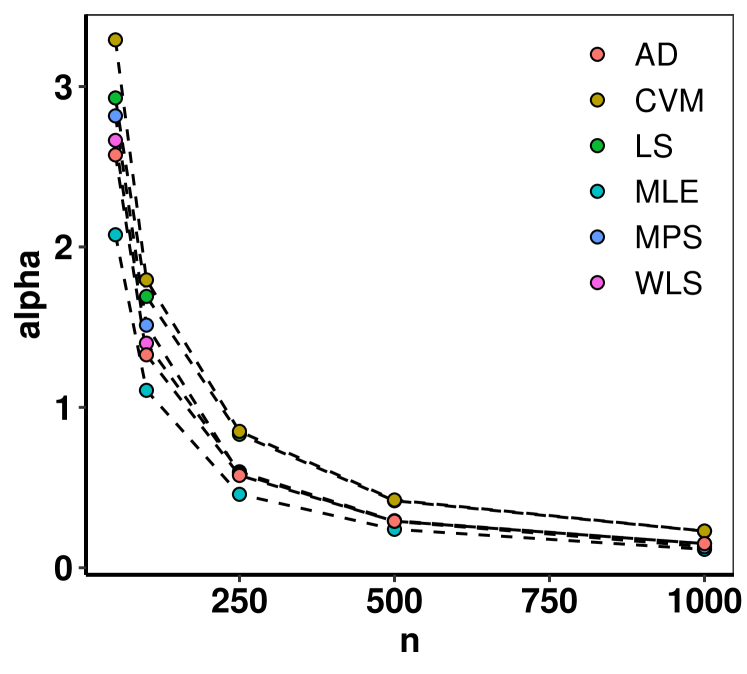
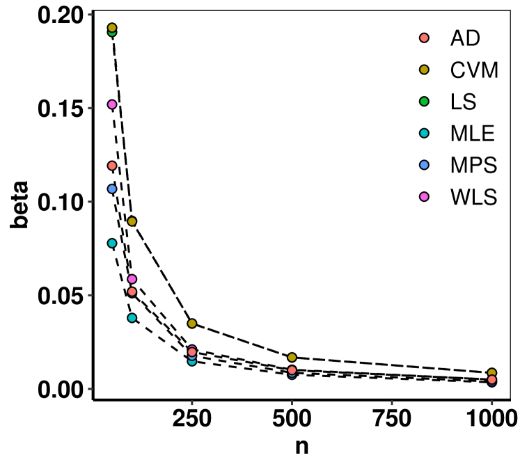
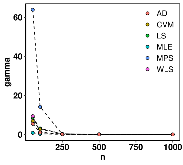
We combined Monte Carlo simulation with the above techniques to estimate the parameters. The parameters are set as $\alpha=2.5,\beta=0.8$, and $\gamma=1.3$. The sample sizes $N=50,100,250,500$, and $1000$ were used to generate random samples. For each sample size, the experiment was replicated for $N=1000$ times. Then the bias and mean squared error (MSE) were calculated. Table 2 and Fig. 1 show the estimation results. The MSE converges to 00 when $N$ increases, confirming the estimations’ stability and reliability.

Refer to caption
Refer to caption
Refer to caption
Figure 1: MSE of parameters in Table 3
Table 2: Different estimations for $\alpha=2.5,\beta=0.8,\gamma=1.3$
MLE LS WLS MPS CVM AD
$N$ Bias MSE Bias MSE Bias MSE Bias MSE Bias MSE Bias MSE
50 $\alpha$ 0.0909 2.0761 -0.0418 2.9292 0.0307 2.6645 0.8349 2.8174 0.1095 3.2913 0.1459 2.5743
$\beta$ 0.0512 0.0778 0.0107 0.1906 0.0066 0.1520 -0.1492 0.1068 0.0262 0.1929 0.0010 0.1192
$\gamma$ 0.1512 0.8690 0.9373 8.7264 0.8477 9.4008 2.4409 63.8413 0.8518 6.9832 0.6359 5.4760
100 $\alpha$ 0.0662 1.1061 0.0595 1.6917 0.0878 1.4001 0.5914 1.5128 0.1357 1.7947 0.1327 1.3275
$\beta$ 0.0182 0.0379 -0.0229 0.0897 -0.0158 0.0586 -0.1047 0.0511 -0.0161 0.0895 -0.0163 0.0520
$\gamma$ 0.0963 0.3519 0.4901 3.1145 0.2684 1.1972 0.8138 14.1750 0.4755 2.7094 0.2518 0.9787
250 $\alpha$ 0.0203 0.4578 0.0211 0.8317 0.0336 0.5983 0.3204 0.5872 0.0510 0.8502 0.0533 0.5754
$\beta$ 0.0097 0.0148 -0.0027 0.0349 -0.0010 0.0211 -0.0544 0.0177 -0.0002 0.0350 -0.0027 0.0197
$\gamma$ 0.0265 0.1085 0.1088 0.3554 0.0614 0.1707 0.2180 0.2020 0.1141 0.3529 0.0660 0.1620
500 $\alpha$ 0.0226 0.2394 0.0168 0.4176 0.0220 0.2933 0.2066 0.2890 0.0318 0.4223 0.0321 0.2900
$\beta$ 0.0049 0.0075 -0.0015 0.0168 0.0002 0.0102 -0.0335 0.0086 -0.0003 0.0168 -0.0008 0.0100
$\gamma$ 0.0189 0.0543 0.0498 0.1280 0.0307 0.0742 0.1269 0.0809 0.0529 0.1282 0.0347 0.0744
1000 $\alpha$ 0.0072 0.1146 0.0071 0.2278 0.0113 0.1497 0.1163 0.1310 0.0146 0.2290 0.0167 0.1504
$\beta$ 0.0027 0.0036 -0.0003 0.0086 0.0001 0.0050 -0.0198 0.0039 0.0003 0.0086 -0.0007 0.0050
$\gamma$ 0.0079 0.0254 0.0258 0.0673 0.0160 0.0373 0.0691 0.0331 0.0274 0.0673 0.0186 0.0380

5 Special Cases

In this section, we will explore a variety of special cases that emerge from our novel distribution model. By closely examining these unique instances, we aim to illustrate the multifaceted aspects and potential applications of the T2GWG family of distributions.

5.1 Type-2 Gumbel Weibull-Exponential (T2GWE) distribution

Suppose the baseline distribution $H(x,\boldsymbol{\psi})$ is an exponential distribution with parameter $\gamma>0$. Then $h(x;\gamma)=\gamma e^{-\gamma x}$ and $H(x;\gamma)=1-e^{-\gamma x}$.

5.1.1 cdf and pdf of the T2GWE distribution

The cdf of the Type-2 Gumbel Weibull-Exponential distribution is presented as

$\displaystyle F_{T2GWE}(x)=\exp\left\{-\alpha(e^{\gamma x}-1)^{-\beta}\right\}$ (48)

and the pdf is given by

$\displaystyle f_{T2GWE}(x)=\beta\alpha(e^{\gamma x}-1)^{-\beta-1}\exp\left\{\gamma x-\alpha(e^{\gamma x}-1)^{-\beta}\right\}$ (49)

where $x\geq 0$ and $\alpha,\beta>0$

5.1.2 Hazard rate and quantile functions

The hrf is shown as

$\displaystyle h_{T2GWE}=\frac{\beta\alpha(e^{\gamma x}-1)^{-\beta-1}\exp\left\{\gamma x-\alpha(e^{\gamma x}-1)^{-\beta}\right\}}{1-\exp\left\{-\alpha(e^{\gamma x}-1)^{-\beta}\right\}}$ (50)

and the reverse hrf is given by

$\displaystyle\tau_{T2GWE}=\beta\alpha(e^{\gamma x}-1)^{-\beta-1}$ (51)

Moreover, the quantile function is obtained as

$\displaystyle x_{p}=-\frac{1}{\gamma}\log\left(\left[\frac{\log p}{-\alpha}\right]^{-\frac{1}{\beta}}+1\right)$ (52)

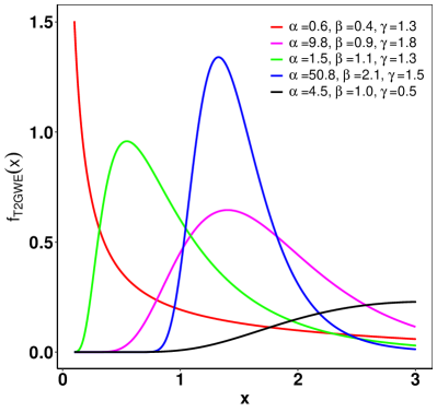
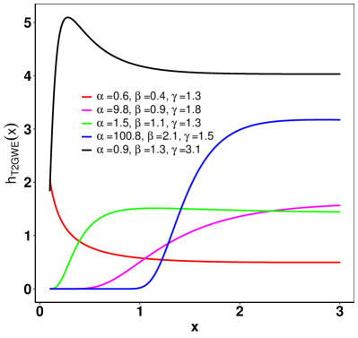
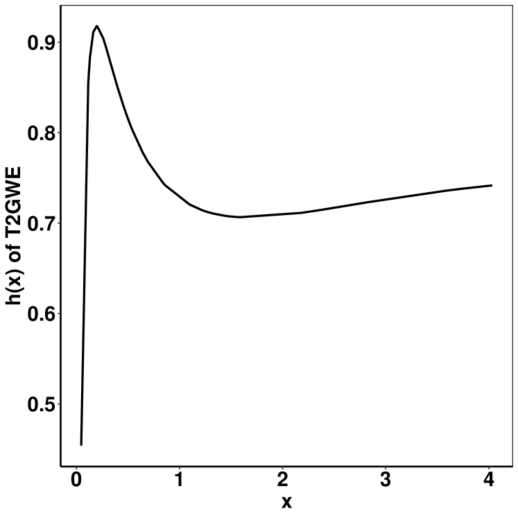
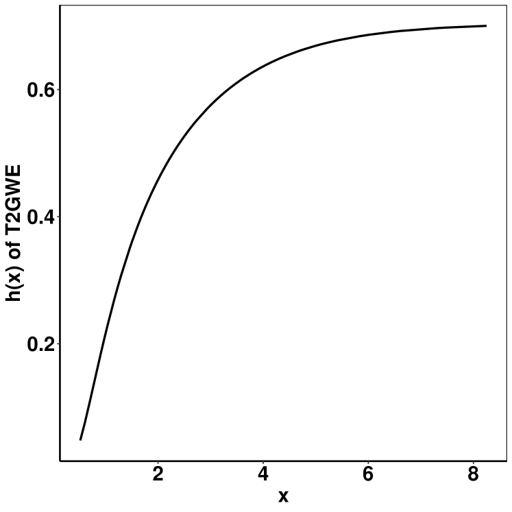
Fig. 2 displays several typical configurations of the pdf and hrf for the T2GWE distribution. The pdf of the T2GWE distribution shows various configurations, including almost symmetric, right-skewed, decreasing, and increasing. Additionally, the hrf of the T2GWE distribution can exhibit a range of shapes, such as decreasing, increasing, and right-skewed.

Refer to caption
Refer to caption
Figure 2: Left: The pdf of T2GWE distribution for different parameters. Right: The hrf of T2GWE for different parameter values.

5.2 Type-2 Gumbel Weibull-Uniform (T2GWU) distribution

Let the baseline distribution $H(x,\boldsymbol{\psi})$ be a uniform distribution with parameter $\gamma>0$. Then $h(x,\gamma)=\frac{1}{\gamma}$ and $H(x,\gamma)=\frac{x}{\gamma}$.

5.2.1 cdf and pdf of the T2GWU distribution

The cdf of the T2GWU distribution is

$\displaystyle F_{T2GWU}=\exp\left\{-\alpha\left(\frac{x}{\gamma-x}\right)^{-\beta}\right\},$ (53)

and the corresponding pdf is

$\displaystyle f_{T2GWU}(x)=\alpha\beta\frac{\gamma x^{-\beta-1}}{(\gamma-x)^{-\beta+1}}\exp\left\{-\alpha\left(\frac{x}{\gamma-x}\right)^{-\beta}\right\}.$ (54)

5.2.2 Hazard rate and quantile functions

The hrf of T2GWU is displayed by

$\displaystyle h_{T2GWU}=\frac{\alpha\beta\frac{\gamma x^{-\beta-1}}{(\gamma-x)^{-\beta+1}}\exp\left\{-\alpha\left(\frac{x}{\gamma-x}\right)^{-\beta}\right\}}{1-\exp\left\{-\alpha\left(\frac{x}{\gamma-x}\right)^{-\beta}\right\}},$ (55)

and the reverse hrf is given by

$\displaystyle\tau_{T2GWU}=\alpha\beta\frac{\gamma x^{-\beta-1}}{(\gamma-x)^{-\beta+1}}.$ (56)

Moreover, the quantile function can be obtained as

$\displaystyle x_{p}=\frac{1}{1+\left[\frac{\log p}{-\alpha}\right]^{\frac{1}{\beta}}}.$ (57)

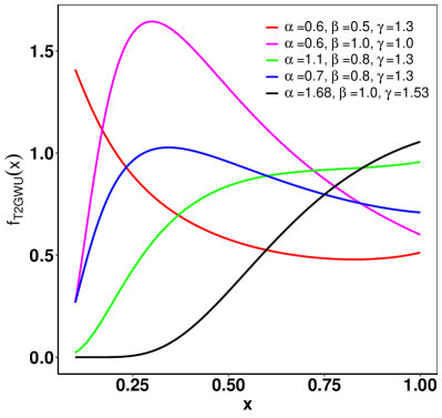
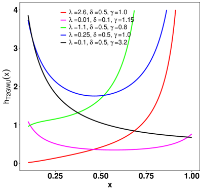
Fig. 3 plots of the pdf and hrf for the T2GWU distribution with several combinations of parameter values. The pdf plots show different shapes, including right-skewed, decreasing, and increasing. In addition, the hrf plots capture various possibilities such as increasing, decreasing, bathtub, and shallow bathtub.

Refer to caption
Refer to caption
Figure 3: Left: pdf of T2GWU distribution for different values of parameters $\alpha$, $\beta$, and $\gamma$. Right: hrf of T2GWU for selected parameters $\alpha$, $\beta$, and $\gamma$.

5.3 Type-2 Gumbel Weibull-Pareto (T2GWP) distribution

If we set $H(x,\boldsymbol{\psi})$ as a Pareto distribution with parameter $\theta,k>0$, then $\displaystyle h(x,\theta,k)=\frac{k\theta^{k}}{x^{k+1}}$ and $\displaystyle H(x,\theta,k)=1-\left(\frac{\theta}{x}\right)^{k}$.

5.3.1 cdf and pdf of the T2GWP distribution

Thus the cdf of the T2GWP distribution is given by

$\displaystyle F_{T2GWP}=\exp\left\{-\alpha\left(\left[\frac{x}{\theta}\right]^{k}-1\right)^{-\beta}\right\},$ (58)

with a pdf

$\displaystyle f_{T2GWP}(x)=\beta\alpha kx^{k-1}\theta^{-k}\left(\left[\frac{x}{\theta}\right]^{k}-1\right)^{-\beta-1}\exp\left\{-\alpha\left(\left[\frac{x}{\theta}\right]^{k}-1\right)^{-\beta}\right\}.$ (59)

5.3.2 Hazard rate and quantile functions

The hrf of T2GWP is displayed by

$\displaystyle h_{T2GWP}=\frac{\beta\alpha kx^{k-1}\theta^{-k}\left(\left[\frac{x}{\theta}\right]^{k}-1\right)^{-\beta-1}\exp\left\{-\alpha\left(\left[\frac{x}{\theta}\right]^{k}-1\right)^{-\beta}\right\}}{1-\exp\left\{-\alpha\left(\left[\frac{x}{\theta}\right]^{k}-1\right)^{-\beta}\right\}},$ (60)

and the reverse hrf is

$\displaystyle\tau_{T2GWP}=\beta\delta\alpha^{-\delta}kx^{k-1}\theta^{-k}\left(\left[\frac{x}{\theta}\right]^{k}-1\right)^{-\beta\delta-1}.$ (61)

Moreover, the quantile function is obtained as

$\displaystyle x_{p}=\theta\left(\left[\frac{\log p}{-\alpha}\right]^{-\frac{1}{\beta}}+1\right)^{\frac{1}{k}}$ (62)

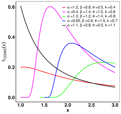
Shapes of the pdf and hrf for the T2GWP distribution with selected parameters are shown in Fig. 4. The pdfs exhibit a variety of shapes including right-skewed, decreasing, and increasing. Moreover, hrf plots for the T2GWP distribution display growing, decreasing, and right-skewed forms.

Refer to caption
Refer to caption
Figure 4: Left: The pdf of T2GWP distribution for selected values of $\alpha$, $\beta$, $\theta$ and $k$. Right: The hrf of T2GWP for various $\alpha$, $\beta$, $\theta$ and $k$.

6 Applications

In this section, we will investigate beyond theoretical constructs and delve into the practical implications of our model, demonstrating its applicability using real-world data sets. This will validate the practical utility of our newly devised model and shed light on how it can be effectively employed in handling concrete data-driven scenarios. The objective is to ensure that our theoretical advancements resonate with tangible applications, thereby significantly contributing to both the academic discourse and the operational applications of statistical distributions.

In this section, we present three applications of the Type-2 Gumbel Weibull-exponential distribution. We compared it with the Exponentiated Gumbel Type-2 (EGT) [28], Weibull Generalized Exponential (WGE) [29], Lomax Gumbel Type-2 (LGT) [30], Type-2 Gumbel (T2G), and with Exponentiated Weibull-Logistic distributions (EWL) [31]. The pdf and cdf of those distributions are provided in Appendix B. The goodness-of-fit statistics including -2log-likelihood statistic, Cramér-von Mises statistic ($W^{*}$), Anderson-Darling statistic ($A^{*}$), Akaike Information Criterion (AIC), Bayesian Information Criterion (BIC), Consistent Akaike Information Criterion (CAIC), Hannan-Quinn criterion (HQIC), Kolmogorov-Smirnov test statistic (K-S) and its corresponding p-value are reported.

To evaluate and compare the performance of different models, we can examine their goodness-of-fit statistics. Generally, a model with smaller values in these statistics fits the data better. However, it’s important to note that for the p-values, which are a measure of expectation, a larger value indicates a better fit.

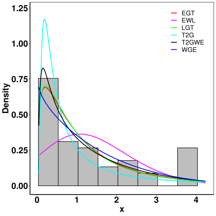
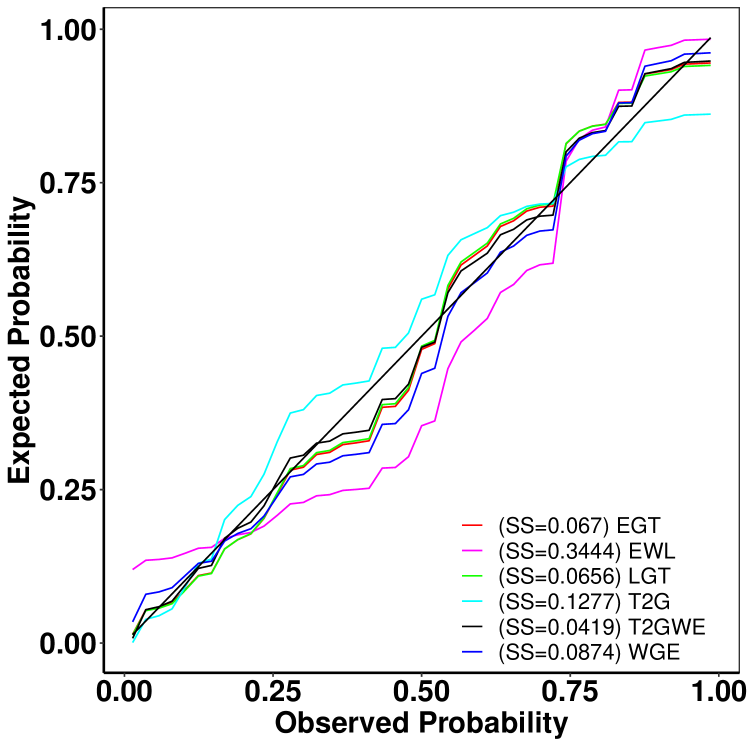
6.1 Chemotherapy data

This dataset is a subset of data reported by Bekker et al. [32], which represents the survival times (in years) of a group of patients who received chemotherapy treatment alone. Please refer to the “Declarations” section for guidance on how to access the data.

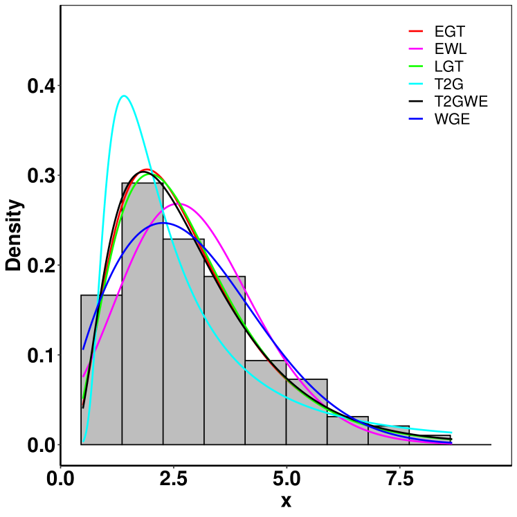
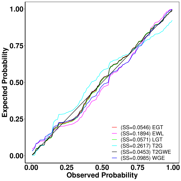
The estimates of the parameters and the goodness-of-fit statistics are summarized in Table 3. Fig. 5 plots of the fitted densities alongside the histogram and the expected probability. From Table 3, we can conclude that the Type-2 Gumbel Weibull-exponential distribution has better performance than other distributions because of its lowest values among all measures of goodness-of-fit and the highest p-value in the K-S test.

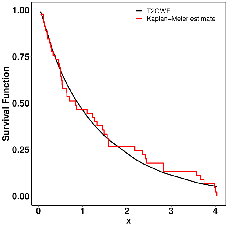
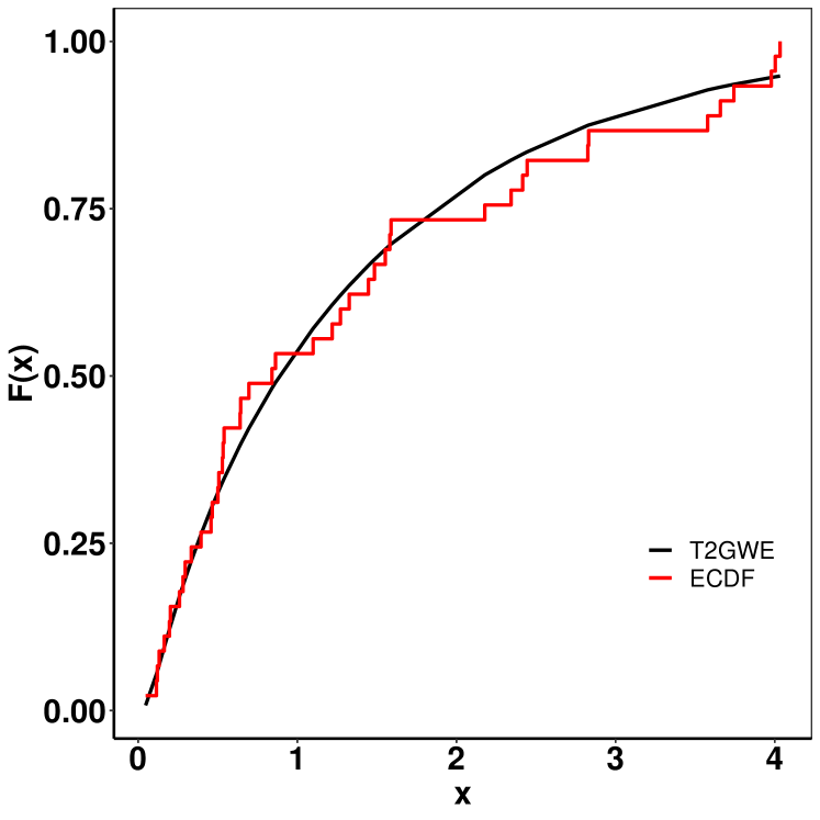
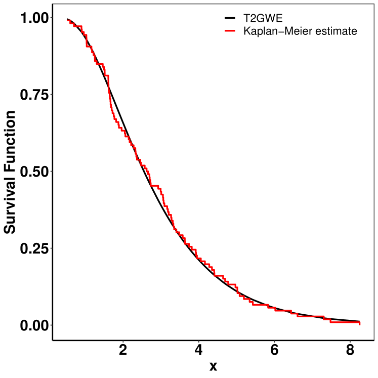
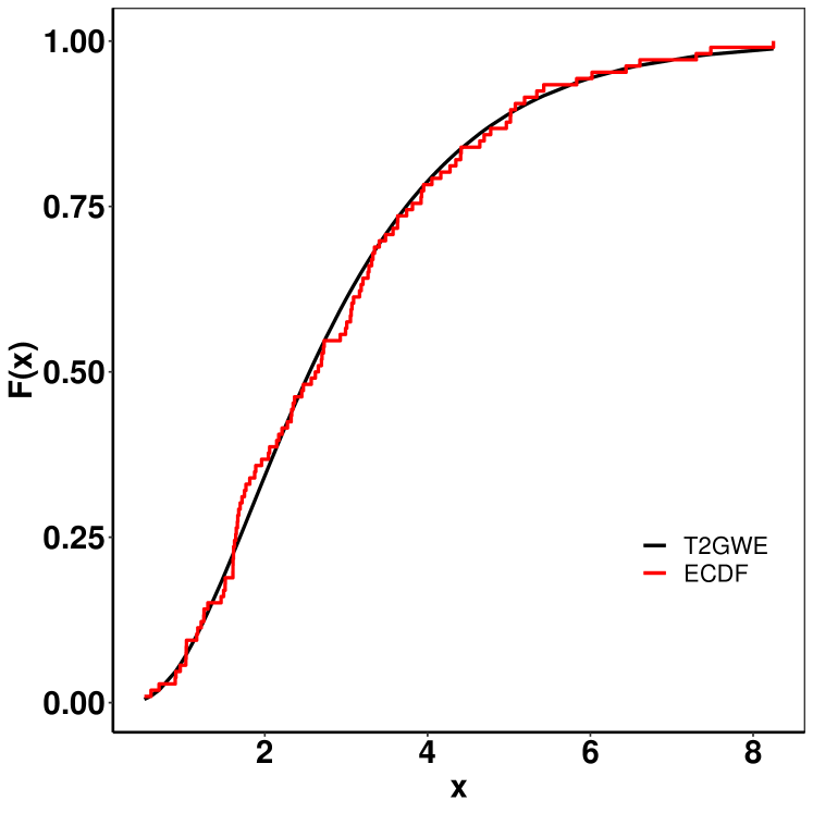
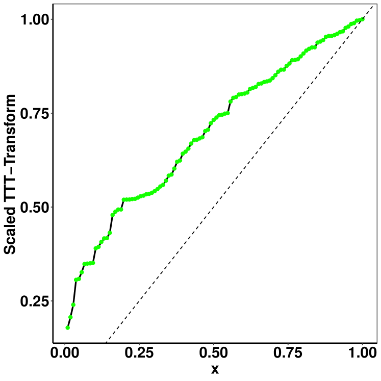
In Fig. 6, the Kaplan-Meier (K–M) survival curve, as well as the theoretical and empirical cumulative distribution functions (ECDF), and total time on test (TTT) scaled are displayed. The closely matched empirical and theoretical plots suggest that our model is an excellent fit for the given data. Additionally, the TTT scaled plot shows that the model is suitable for a hazard rate structure that is not monotonic.

Refer to caption
Refer to caption
Figure 5: left) Fitted density superposed on the histogram and observed probability for the Chemotherapy data. right) Expected probability plots for the Chemotherapy data.
Refer to caption
Refer to caption
Refer to caption
Refer to caption
Figure 6: Fitted K-M survival curve, theoretical and ECDF, the TTT statistics, and the hrf for the Chemotherapy data.
Table 3: MLEs and Goodness-of-Fit Statistics for Chemotherapy Data
Estimates (SE) Statistics
Model $\alpha$ $\beta$ $\gamma$ $-2\log\,L$ $AIC$ $CAIC$ $BIC$ $HQIC$ $W^{*}$ $A^{*}$ K-S p-value
T2GWE 1.1328 0.5416 1.4015 - 113.3334 119.3334 119.9188 124.7534 121.3539 0.0415 0.3113 0.0756 0.9421
(0.4388) (0.1170) (0.5530)
$\alpha$ $\phi$ $\theta$
EGT 1000.1282 0.1452 7.1554 - 115.9096 121.9096 122.4949 127.3295 123.9301 0.0608 0.4231 0.0927 0.0926
($3.6913\times 10^{3}$) ($7.4598\times 10^{-2}$) (3.7373)
$\alpha$ $\theta$ $\gamma$
WGE 3.9393 0.9508 0.1484 - 115.9251 121.9251 122.5105 127.3451 123.9457 0.0917 0.6079 0.1120 0.5864
(8.8328) (0.2076) (0.2675)
$\alpha$ $\beta$ $\theta$ $k$
LGT 17.9903 0.0196 7.0332 0.1503 116.3564 124.3564 125.3564 131.5831 127.0504 0.0610 0.4270 0.0892 0.835
(24.8990) (0.0298) (1.9777) (0.0459)
$\alpha$ $\nu$
T2G 0.4987 0.8672 - - 127.6381 131.6381 131.9238 135.2515 132.9851 0.1430 0.9790 0.1382 0.3253
(0.0979) (0.0928)
$\alpha$ $\beta$ $\lambda$ $\theta$
EWL 4.6147 0.3981 0.4506 221.7210 140.0032 148.0032 149.0032 155.2298 150.6972 0.3318 2.0776 0.1853 0.0796
(1.1065) (0.6466) (0.7320) (250.5359)

6.2 Depressive data

This dataset consists of scores from the “General Rating of Affective Symptoms for Preschoolers” (GRASP) scale, which is used to assess behavioral and emotional problems in children. The data set is studied by [33]. Please refer to the “Declarations” section for detailed instructions on how to access the data.

From Table 4 and Fig. 7, we can conclude that the Type-2 Gumbel Weibull-exponential distribution has better performance than other distributions as it possesses the smallest values for all goodness-of-fit statistics and the highest p-value in the K-S test. As shown in Fig. 8, the close resemblance between the fitted empirical and theoretical plots indicates a strong fit of our model to the provided data. Furthermore, the TTT scaled plot provides clear evidence that the model is appropriate for a non-monotonic hazard rate structure.

Refer to caption
Refer to caption
Figure 7: left) Fitted density superposed on the histogram and observed probability for the Depressive data. right) Expected probability plots for the Depressive data.
Refer to caption
Refer to caption
Refer to caption
Refer to caption
Figure 8: Fitted K-M survival curve, theoretical and ECDF, the TTT statistics, and the hrf for the Depressive data.
Table 4: MLEs and Goodness-of-Fit Statistics for Depressive Data
Estimates (SE) Statistics
Model $\alpha$ $\beta$ $\gamma$ $-2\log\,L$ $AIC$ $CAIC$ $BIC$ $HQIC$ $W^{*}$ $A^{*}$ K-S p-value
T2GWE 0.1127 5.0122 0.0223 - 785.7463 791.7463 791.9309 800.4398 795.2791 0.1814 1.3478 0.1092 0.0821
(0.0818) (0.3542) (0.0024)
$\alpha$ $\phi$ $\theta$
EGT 9.7621 2.0192 1691.0601 - 803.2078 809.2078 809.3924 817.9013 812.7406 0.3185 2.1927 0.1108 0.0746
(3.7163) (0.2403) (1088.5591)
$\alpha$ $\theta$ $\gamma$
WGE 44.2733 3.7778 0.0115 - 852.253 858.253 858.4376 866.9465 861.7858 0.8203 5.0577 0.1913 0.0001
(163.1340) (0.5147) (0.0008)
$\alpha$ $\beta$ $\theta$ $k$
LGT 2.7374 0.0006 161.2461 1.0193 807.7372 815.7372 816.0473 827.3286 820.4476 0.3392 2.3111 0.1252 0.0301
(0.9395) (0.0028) (46.6043) (0.1060)
$\alpha$ $\nu$
T2G 1684.3935 2.3918 - - 919.7708 923.7708 923.8624 929.5665 926.126 0.2340 1.6765 0.2480 $1.392e-07$
(404.6525) (0.0807)
$\alpha$ $\beta$ $\lambda$ $\theta$
EWL 1.2679 0.0770 0.6636 61.1849 816.1935 824.1935 824.5036 835.7849 828.9039 0.4525 2.9886 0.1310 0.0202
(0.3130) (0.0271) (0.2349) (31.6238)

6.3 Covid-Mexico data

This dataset recorded the mortality rates of the patients infected by the COVID-19 pandemic in Mexico and was studied by [34]. This dataset consists of 106 observations from March 31, 2020, to July 20, 2020. To access the data, please follow the instructions in the “Declarations” section.

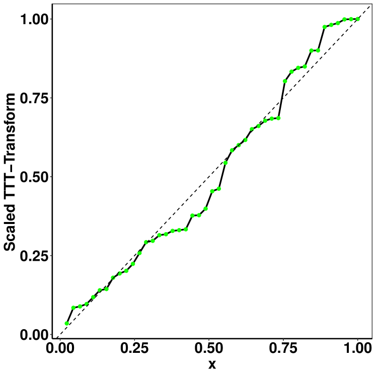
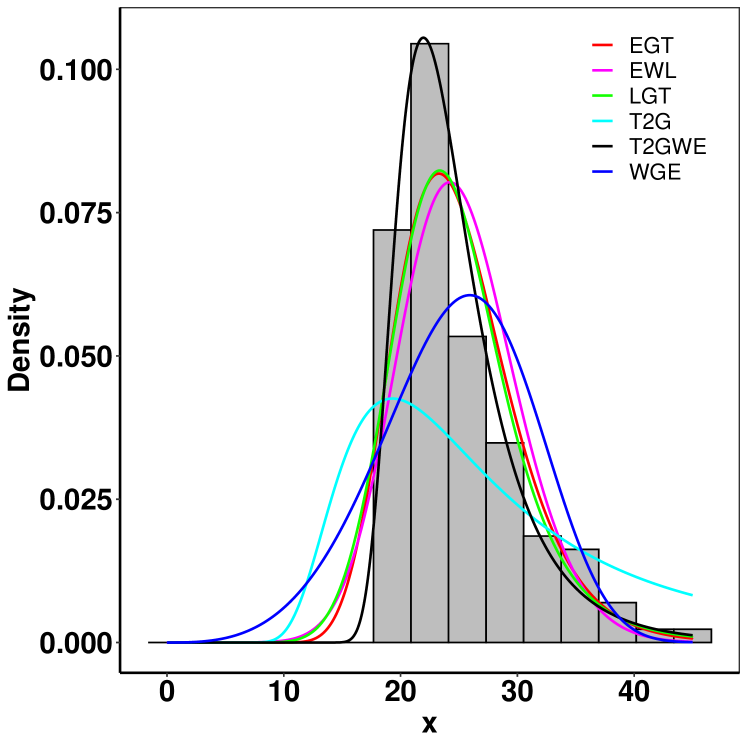
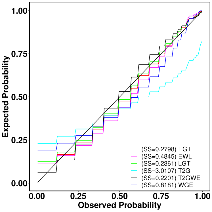
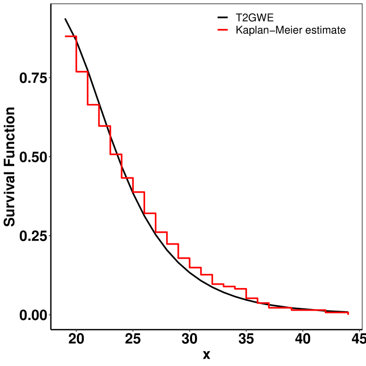
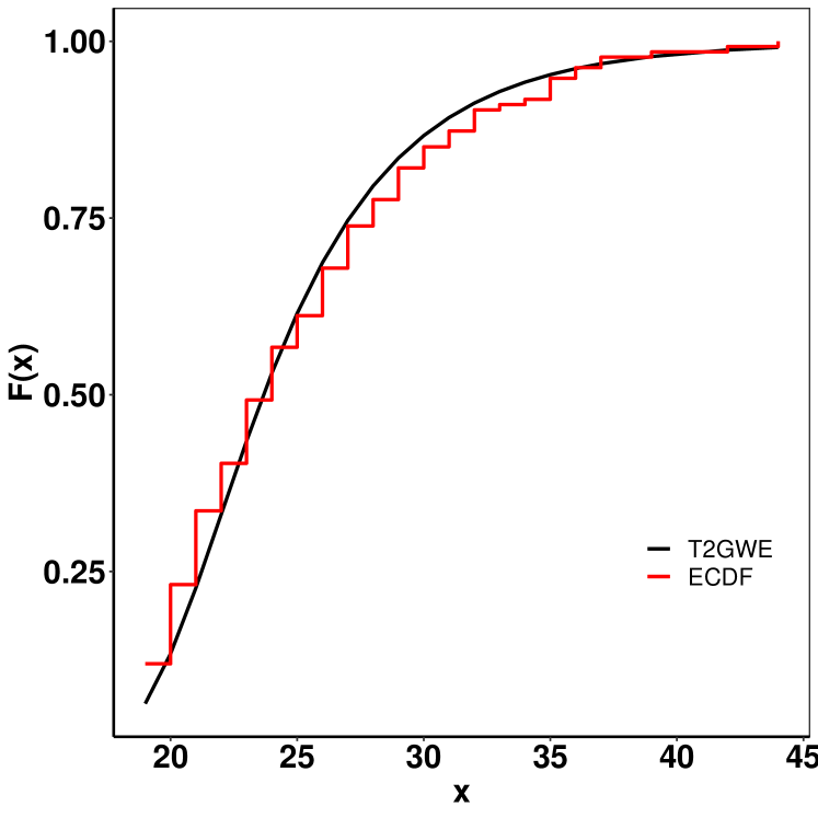
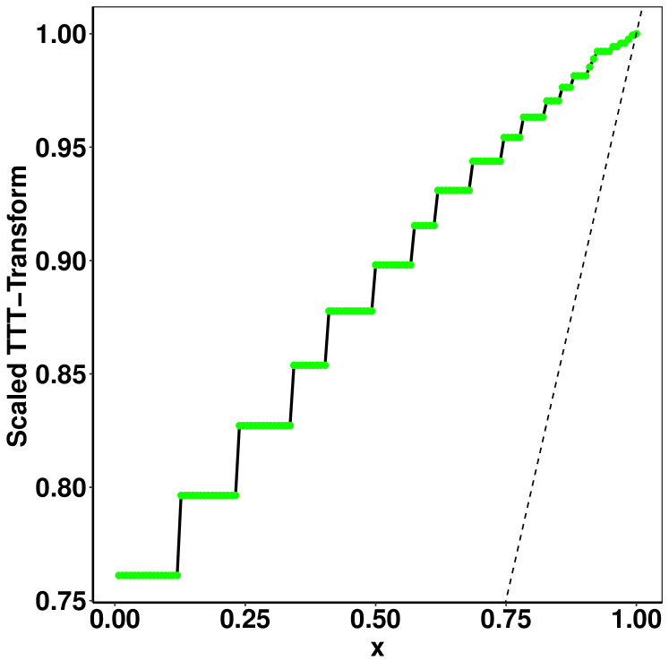
Table 5 and Fig. 9 provide the estimates of the parameters and the goodness-of-fit. We can conclude that the Type-2 Gumbel Weibull-exponential distribution has the best performance among other distributions given its smallest values in all goodness-of-fit statistics and the highest p-value in the K-S test. Displayed in Fig. 10 are the K-M survival curve, as well as the theoretical and ECDF, and TTT scaled. The convergence of the fitted empirical and theoretical plots suggests that our model accurately represents the given data. In addition, the TTT scaled plot clearly indicates that the model is well-suited for a hazard rate structure that is not strictly monotonic.

Refer to caption
Refer to caption
Figure 9: left) Fitted density superposed on the histogram and observed probability for the Covid-Mexico data. right) Expected probability plots for the Covid-Mexico data.
Refer to caption
Refer to caption
Refer to caption
Refer to caption
Figure 10: Fitted K-M survival curve, theoretical and ECDF functions, the TTT statistics, and the hrf for the Covid-Mexico data.
Table 5: MLEs and Goodness-of-Fit Statistics for Covid-Mexico Data
Estimates (SE) Statistics
Model $\alpha$ $\beta$ $\gamma$ $-2\log\,L$ $AIC$ $CAIC$ $BIC$ $HQIC$ $W^{*}$ $A^{*}$ K-S p-value
T2GWE 3.9220 0.7209 0.9767 - 375.7089 381.7089 381.9442 389.6993 384.9475 0.0454 0.2525 0.0577 0.8721
(1.4023) (0.2117) (0.3942)
$\alpha$ $\phi$ $\theta$
EGT 56.8310 0.4537 6.7577 - 376.3527 382.3527 382.5879 390.343 385.5912 0.0521 0.2877 0.0646 0.7686
(78.7004) (0.1409) (1.3261)
$\alpha$ $\theta$ $\gamma$
WGE 49.8868 1.8037 0.0326 - 382.8119 388.8119 389.0472 396.8022 392.0504 0.1128 0.7313 0.0664 0.7387
(72.3253) (0.1413) (0.0222)
$\alpha$ $\beta$ $\theta$ $k$
LGT 11.9707 0.0343 8.5300 0.3374 376.8091 384.8091 385.2052 395.4629 389.1271 0.0557 0.3106 0.0688 0.6975
(11.5930) (0.0615) (1.6317) (0.0982)
$\alpha$ $\nu$
T2G 2.8185 1.6830 - - 400.2692 404.2692 404.3857 409.5961 406.4282 0.2734 1.7490 0.0928 0.3213
(0.2928) (0.1163)
$\alpha$ $\beta$ $\lambda$ $\theta$
EWL 3.6179 0.3384 0.4196 150.8827 390.9746 398.9747 399.3707 409.6284 403.2927 0.1807 1.1892 0.0957 0.2857
(0.6784) (2.5979) (3.2208) (109.2607)

7 Conclusion

This paper introduces a novel methodology for generating continuous statistical distributions by utilizing the exponentiated odds ratio, which is based on the concepts of survival analysis. The approach described herein constitutes a substantial advancement in the field of statistical modeling, effectively augmenting the flexibility and accuracy of distribution models to effectively address the requirements posed by intricate contemporary data architectures. The major point of this progress lies in the formulation of the “Type-2 Gumbel Weibull-G Family of Distributions,” which has undergone a comprehensive mathematical analysis. The scope of this investigation covered various statistical properties, such as expansions of density functions, moments, hazard rate and quantile functions, Rényi entropy, order statistics, and an examination of stochastic ordering.

In order to assess the robustness and reliability of the new generator, we employed a set of five advanced parameter estimation techniques: Maximum Likelihood, Least Square, Weighted Least Square, Maximum Product Spacing, Cramér-von Mises, and Anderson and Darling. The efficacy and utility of the Type-2 Gumbel Weibull-G distributions were further validated through a comprehensive analysis of three datasets obtained from real-world scenarios. These practical implementations demonstrated the superior statistical accuracy of our proposed distributions over existing models, thereby emphasizing their relevance and applicability in both theoretical and practical statistical domains.

Our future research endeavors will entail a thorough investigation of several sub-families within the new generator. This exploration will focus on their distinct properties and potential applications in diverse scenarios, setting them in comparison with other established distribution models. Furthermore, we are now developing an R package with the objective of optimizing the parameter estimate process through the utilization of diverse methodologies. This will result in improved efficiency of data-fitting procedures, thus increasing the accessibility and practicality of our study for wider applications.

Abbreviations

The following abbreviations are used in this paper:

T2GWG The Type-2 Gumbel Weibull-G
cdf cumulative distribution function
pdf probability density function
hrf hazard rate function
Exp-G exponentiated-G
EGT Exponentiated Gumbel Type-2
WGE Weibull Generalized Exponential
LGT Lomax Gumbel Type-2
T2G Type-2 Gumbel
EWL Exponentiated Weibull-Logistic distributions
MLE maximum likelihood estimates
MPS maximum product spacing estimates
LS least square estimates
WLS weighted least square estimates
CVM Cramér-von Mises estimates
AD Anderson and Darling estimates
T2GWE Type-2 Gumbel Weibull-Exponential
T2GWU Type-2 Gumbel Weibull-Uniform
T2GWP Type-2 Gumbel Weibull-Pareto
AIC Akaike Information Criterion
CAIC Consistent Akaike Information Criterion
BIC Bayesian Information Criterion
HQIC Hannan-Quinn Criterion
$W^{*}$ Cramér-von Mises statistic
$A^{*}$ Anderson-Darling statistic
K-S Kolmogorov-Smirnov statistic
ECDF empirical cumulative distribution function
TTT total time on test
K-M Kaplan-Meier
\bmhead

Supplementary information Not applicable

\bmhead

Acknowledgments

The authors wish to thank all members of the CSDA lab at the University of West Florida for their helpful comments on the manuscript.

Declarations

  • Funding: This research received no specific grant from any funding agency in the public, commercial, or not-for-profit sectors.

  • Conflict of interest/Competing interests: On behalf of all authors, the corresponding author states that there is no conflict of interest.

  • Ethics approval: Not applicable

  • Consent to participate: Not applicable

  • Consent for publication: Not applicable

  • Availability of data and materials: All data utilized in this study is openly available on GitHub. The dataset can be accessed through the provided link: https://github.com/shusenpu/Generator_Data. The data can also be accessed using its Digital Object Identifier (DOI): 10.5281/zenodo.10215787. To retrieve the data, visit the following link: https://doi.org/10.5281/zenodo.10215787.

  • Code availability: available upon request.

  • Authors’ contributions: All authors have contributed significantly to writing and editing the paper.

Appendix A The first derivatives of H

The first partial derivatives of $H$ in Section 4 with respect to $\alpha,\beta,\delta,\psi_{k}$ are given by

$\displaystyle\frac{\partial H}{\partial\alpha}=$ $\displaystyle\frac{1}{n+1}\left\{-\left[\frac{H(x_{1},\boldsymbol{\psi})}{\overline{H}(x_{1},\boldsymbol{\psi})}\right]^{-\beta}+\frac{\left[\frac{H(x_{n},\boldsymbol{\psi})}{\overline{H}(x_{n},\boldsymbol{\psi})}\right]^{-\beta}\exp\left\{-\alpha\left[\frac{H(x_{i},\boldsymbol{\psi})}{\overline{H}(x_{i},\boldsymbol{\psi})}\right]^{-\beta}\right\}}{1-\exp\left\{-\alpha\left[\frac{H(x_{i},\boldsymbol{\psi})}{\overline{H}(x_{i},\boldsymbol{\psi})}\right]^{-\beta}\right\}}\right.$
$\displaystyle+\sum_{i=2}^{n}\left[\frac{\left[\frac{H(x_{i},\boldsymbol{\psi})}{\overline{H}(x_{i},\boldsymbol{\psi})}\right]^{-\beta}\exp\left\{-\alpha\left[\frac{H(x_{i},\boldsymbol{\psi})}{\overline{H}(x_{i},\boldsymbol{\psi})}\right]^{-\beta}\right\}}{\exp\left\{-\alpha\left[\frac{H(x_{i},\boldsymbol{\psi})}{\overline{H}(x_{i},\boldsymbol{\psi})}\right]^{-\beta}\right\}-\exp\left\{-\alpha\left[\frac{H(x_{i-1},\boldsymbol{\psi})}{\overline{H}(x_{i-1},\boldsymbol{\psi})}\right]^{-\beta}\right\}}\right.$
$\displaystyle\left.\left.-\frac{\left[\frac{H(x_{i-1},\boldsymbol{\psi})}{\overline{H}(x_{i-1},\boldsymbol{\psi})}\right]^{-\beta}\exp\left\{-\alpha\left[\frac{H(x_{i-1},\boldsymbol{\psi})}{\overline{H}(x_{i-1},\boldsymbol{\psi})}\right]^{-\beta}\right\}}{\exp\left\{-\alpha\left[\frac{H(x_{i},\boldsymbol{\psi})}{\overline{H}(x_{i},\boldsymbol{\psi})}\right]^{-\beta}\right\}-\exp\left\{-\alpha\left[\frac{H(x_{i-1},\boldsymbol{\psi})}{\overline{H}(x_{i-1},\boldsymbol{\psi})}\right]^{-\beta}\right\}}\right]\right\}$ (63)
$\displaystyle\frac{\partial H}{\partial\beta}=$ $\displaystyle\frac{1}{n+1}\left\{\alpha\log\left(\frac{H(x_{1},\boldsymbol{\psi})}{\overline{H}(x_{1},\boldsymbol{\psi})}\right)\left[\frac{H(x_{i},\boldsymbol{\psi})}{\overline{H}(x_{i},\boldsymbol{\psi})}\right]^{-\beta}\right.$
$\displaystyle+\frac{\log\left(\frac{H(x_{n},\boldsymbol{\psi})}{\overline{H}(x_{n},\boldsymbol{\psi})}\right)\left[\frac{H(x_{n},\boldsymbol{\psi})}{\overline{H}(x_{n},\boldsymbol{\psi})}\right]^{-\beta}\exp\left\{-\alpha\left[\frac{H(x_{i},\boldsymbol{\psi})}{\overline{H}(x_{i},\boldsymbol{\psi})}\right]^{-\beta}\right\}}{1-\exp\left\{-\alpha\left[\frac{H(x_{i},\boldsymbol{\psi})}{\overline{H}(x_{i},\boldsymbol{\psi})}\right]^{-\beta}\right\}}$
$\displaystyle+\sum_{i=2}^{n}\left[\frac{\log\left(\frac{H(x_{i},\boldsymbol{\psi})}{\overline{H}(x_{i},\boldsymbol{\psi})}\right)\left[\frac{H(x_{i},\boldsymbol{\psi})}{\overline{H}(x_{i},\boldsymbol{\psi})}\right]^{-\beta}\exp\left\{-\alpha\left[\frac{H(x_{i},\boldsymbol{\psi})}{\overline{H}(x_{i},\boldsymbol{\psi})}\right]^{-\beta}\right\}}{\exp\left\{-\alpha\left[\frac{H(x_{i},\boldsymbol{\psi})}{\overline{H}(x_{i},\boldsymbol{\psi})}\right]^{-\beta}\right\}-\exp\left\{-\alpha\left[\frac{H(x_{i-1},\boldsymbol{\psi})}{\overline{H}(x_{i-1},\boldsymbol{\psi})}\right]^{-\beta}\right\}}\right.$
$\displaystyle\left.\left.\left.-\frac{\log\left(\frac{H(x_{i-1},\boldsymbol{\psi})}{\overline{H}(x_{i-1},\boldsymbol{\psi})}\right)\left[\frac{H(x_{i-1},\boldsymbol{\psi})}{\overline{H}(x_{i-1},\boldsymbol{\psi})}\right]^{-\beta}\exp\left\{-\alpha\left[\frac{H(x_{i-1},\boldsymbol{\psi})}{\overline{H}(x_{i-1},\boldsymbol{\psi})}\right]^{-\beta}\right\}}{\exp\left\{-\alpha\left[\frac{H(x_{i},\boldsymbol{\psi})}{\overline{H}(x_{i},\boldsymbol{\psi})}\right]^{-\beta}\right\}-\exp\left\{-\alpha\left[\frac{H(x_{i-1},\boldsymbol{\psi})}{\overline{H}(x_{i-1},\boldsymbol{\psi})}\right]^{-\beta}\right\}}\right]\right)\right\}$ (64)
$\displaystyle\frac{\partial H}{\partial\psi_{k}}=$ $\displaystyle\frac{1}{n+1}\left\{\alpha\beta\frac{H(x_{1},\boldsymbol{\psi})^{-\beta-1}}{\overline{H}(x_{1},\boldsymbol{\psi})^{-\beta+1}}\frac{\partial H(x_{1},\boldsymbol{\psi})}{\partial\psi_{k}}+\frac{\frac{H(x_{n},\boldsymbol{\psi})^{-\beta-1}}{\overline{H}(x_{n},\boldsymbol{\psi})^{-\beta+1}}\frac{\partial H(x_{n},\boldsymbol{\psi})}{\partial\psi_{k}}\exp\left\{-\alpha\left[\frac{H(x_{n},\boldsymbol{\psi})}{\overline{H}(x_{n},\boldsymbol{\psi})}\right]^{-\beta}\right\}}{1-\exp\left\{-\alpha\left[\frac{H(x_{n},\boldsymbol{\psi})}{\overline{H}(x_{n},\boldsymbol{\psi})}\right]^{-\beta}\right\}}\right.$
$\displaystyle+\sum_{i=2}^{n}\left[\frac{\frac{H(x_{i},\boldsymbol{\psi})^{-\beta-1}}{\overline{H}(x_{i},\boldsymbol{\psi})^{-\beta+1}}\frac{\partial H(x_{i},\boldsymbol{\psi})}{\partial\psi_{k}}\exp\left\{-\alpha\left[\frac{H(x_{i},\boldsymbol{\psi})}{\overline{H}(x_{i},\boldsymbol{\psi})}\right]^{-\beta}\right\}}{\exp\left\{-\alpha\left[\frac{H(x_{i},\boldsymbol{\psi})}{\overline{H}(x_{i},\boldsymbol{\psi})}\right]^{-\beta}\right\}-\exp\left\{-\alpha\left[\frac{H(x_{i-1},\boldsymbol{\psi})}{\overline{H}(x_{i-1},\boldsymbol{\psi})}\right]^{-\beta}\right\}}\right.$
$\displaystyle\left.\left.\left.-\frac{\frac{H(x_{i-1},\boldsymbol{\psi})^{-\beta-1}}{\overline{H}(x_{i-1},\boldsymbol{\psi})^{-\beta+1}}\frac{\partial H(x_{i-1},\boldsymbol{\psi})}{\partial\psi_{k}}\exp\left\{-\alpha\left[\frac{H(x_{i-1},\boldsymbol{\psi})}{\overline{H}(x_{i-1},\boldsymbol{\psi})}\right]^{-\beta}\right\}}{\exp\left\{-\alpha\left[\frac{H(x_{i},\boldsymbol{\psi})}{\overline{H}(x_{i},\boldsymbol{\psi})}\right]^{-\beta}\right\}-\exp\left\{-\alpha\left[\frac{H(x_{i-1},\boldsymbol{\psi})}{\overline{H}(x_{i-1},\boldsymbol{\psi})}\right]^{-\beta}\right\}}\right]\right)\right\}$ (65)

Appendix B Distributions Used in the Application Section

  • Exponentiated Gumbel Type-2 Distribution:

    $$F_{{}_{EGT}}(x)=1-\left(1-e^{-\theta x^{-\phi}}\right)^{\alpha},$$
    $$f_{{}_{EGT}}(x)=\alpha\phi\theta x^{-\phi-1}e^{-\theta x^{-\phi}}\left(1-e^{-\theta x^{-\phi}}\right)^{\alpha-1},$$
    $$\alpha,\phi,\theta>0$$
  • Weibull Generalized Exponential Distribution:

    $$F_{{}_{WGE}}(x)=1-e^{-a\left[e^{\lambda x}-1\right]^{b}},$$
    $$f_{{}_{WGE}}(x)=ab\lambda e^{\lambda x}\left[e^{\lambda x}-1\right]^{b-1}e^{-a\left[e^{\lambda x}-1\right]^{b}},$$
    $$a,b,\lambda>0$$
  • Lomax Gumbel Type-2 Distribution:

    $$F_{{}_{LGT}}(x)=1-\beta^{\alpha}\left(\beta-\log\left[1-e^{-\theta x^{-k}}\right]\right)^{-\alpha}$$
    $$f_{{}_{LGT}}(x)=\frac{\alpha\beta^{\alpha}\theta kx^{-k-1}e^{-\theta x^{-k}}}{\left[1-e^{-\theta x^{-k}}\right]}\left[\beta-\log\left[1-e^{-\theta x^{-k}}\right]\right]^{-(\alpha+1)}$$
    $$\alpha,\beta,\theta,k>0$$
  • Type-2 Gumbel Distribution:

    $$F_{{}_{T2G}}(x)=e^{-\theta x^{-\phi}}$$
    $$f_{{}_{T2G}}(x)=\phi\theta x^{-\phi-1}e^{-\theta x^{-\phi}}$$
    $$\phi,\theta>0$$
  • Exponentiated Weibull-Logistic Distribution:

    $$F_{{}_{EWL}}(x)=\left(1-e^{-\alpha e^{\lambda\beta x}}\right)^{\theta}$$
    $$f_{{}_{EWL}}(x)=\theta\left(1-e^{-\alpha e^{\lambda\beta x}}\right)^{\theta-1}\left(\lambda\alpha\beta e^{\lambda\beta x-\alpha e^{\lambda\beta x}}\right),$$
    $$\lambda,\alpha,\beta,\theta>0.$$

References

  • \bibcommenthead
  • Rodríguez González et al. [2023] Rodríguez González, C.A., Rodríguez-Pérez, A.M., López, R., Hernández-Torres, J.A., Caparrós-Mancera, J.J.: Sensitivity analysis in mean annual sediment yield modeling with respect to rainfall probability distribution functions. Land 12(1) (2023) https://doi.org/10.3390/land12010035
  • Jiang et al. [2023] Jiang, S.-H., Liu, X., Wang, Z.Z., Li, D.-Q., Huang, J.: Efficient sampling of the irregular probability distributions of geotechnical parameters for reliability analysis. Structural Safety 101, 102309 (2023) https://doi.org/10.1016/j.strusafe.2022.102309
  • Cooray [2006] Cooray, K.: Generalization of the weibull distribution: the odd weibull family. Statistical Modelling 6(3), 265–277 (2006)
  • Bourguignon et al. [2014] Bourguignon, M., Silva, R.B., Cordeiro, G.M.: The weibull-g family of probability distributions. Journal of data science 12(1), 53–68 (2014)
  • Pu et al. [2016] Pu, S., Oluyede, B.O., Qiu, Y., Linder, D.: A generalized class of exponentiated modified Weibull distribution with applications. Journal of Data Science 14(4), 585–613 (2016)
  • Oluyede et al. [2018] Oluyede, B., Pu, S., Makubate, B., Qiu, Y.: The gamma-Weibull-G family of distributions with applications. Austrian Journal of Statistics 47(1), 45–76 (2018)
  • Oluyede and Moakofi [2023] Oluyede, B., Moakofi, T.: The gamma-topp-leone-type ii-exponentiated half logistic-g family of distributions with applications. Stats 6(2), 706–733 (2023)
  • Shama et al. [2023] Shama, M.S., Alharthi, A.S., Almulhim, F.A., Gemeay, A.M., Meraou, M.A., Mustafa, M.S., Hussam, E., Aljohani, H.M.: Modified generalized weibull distribution: theory and applications. Scientific Reports 13(1), 12828 (2023)
  • Emam and Tashkandy [2023] Emam, W., Tashkandy, Y.: Modeling the amount of carbon dioxide emissions application: New modified alpha power weibull-x family of distributions. Symmetry 15(2), 366 (2023)
  • Gabanakgosi and Oluyede [2023] Gabanakgosi, M., Oluyede, B.: The topp-leone type ii exponentiated half logistic-g family of distributions with applications. International Journal of Mathematics in Operational Research 25(1), 85–117 (2023)
  • Sun et al. [2023] Sun, J., Kong, M., Pal, S.: The modified-half-normal distribution: Properties and an efficient sampling scheme. Communications in Statistics-Theory and Methods 52(5), 1591–1613 (2023)
  • Guptha and Maruthan [2023] Guptha, R.C.S., Maruthan, S.K.: A new generalization of power lindley distribution and its applications. Thailand Statistician 21(1), 196–208 (2023)
  • Pu et al. [2023] Pu, S., Moakofi, T., Oluyede, B.: The Ristić–Balakrishnan–Topp–Leone–Gompertz-G family of distributions with applications. Journal of Statistical Theory and Applications, 1–35 (2023)
  • Kajuru et al. [2023] Kajuru, J., Dikko, H., Mohammed, A., Fulatan, A.: Odd gompertz-g family of distribution, its properties and applications. FUDMA JOURNAL OF SCIENCES 7(3), 351–358 (2023)
  • Osagie et al. [2023] Osagie, S.A., Uyi, S., Osemwenkhae, J.E.: The inverse burr-generalized family of distributions: Theory and applications. Earthline Journal of Mathematical Sciences 13(2), 313–351 (2023)
  • Marasigan [2023] Marasigan, A.E.: A new extension of the inverse paralogistic distribution using gamma generator with application. Mindanao Journal of Science and Technology 21(1) (2023)
  • Azimi and Esmailian [2023] Azimi, R., Esmailian, M.: A new generalization of nadarajah-haghighi distribution with application to cancer and covid-19 deaths data. Mathematica Slovaca 73(1), 221–244 (2023)
  • Kleinbaum and Klein [1996] Kleinbaum, D.G., Klein, M.: Survival Analysis a Self-learning Text. Springer, ??? (1996)
  • Tsiatis et al. [2023] Tsiatis, A.A., Davidian, M., Holloway, S.T.: Estimation of the odds ratio in a proportional odds model with censored time-lagged outcome in a randomized clinical trial. Biometrics 79(2), 975–987 (2023)
  • VanderWeele [2020] VanderWeele, T.J.: Optimal approximate conversions of odds ratios and hazard ratios to risk ratios. Biometrics 76(3), 746–752 (2020)
  • Penner et al. [2019] Penner, C.G., Gerardy, B., Ryan, R., Williams, M.: The odds ratio product (an objective sleep depth measure): Normal values, repeatability, and change with cpap in patients with osa: The odds ratio product. Journal of Clinical Sleep Medicine 15(8), 1155–1163 (2019)
  • Alzaatreh et al. [2013] Alzaatreh, A., Carl, L., Felix, F.: A new method for generating families of continuous distributions. Metron, 63–79 (2013)
  • Rényi et al. [1961] Rényi, A., et al.: On measures of entropy and information. In: Proceedings of the Fourth Berkeley Symposium on Mathematical Statistics and Probability, vol. 1, pp. 547–561 (1961). Berkeley, California, USA
  • Szekli [2012] Szekli, R.: Stochastic Ordering and Dependence in Applied Probability vol. 97. Springer, New York (2012)
  • Cheng and Amin [1983] Cheng, R.C.H., Amin, N.A.K.: Estimating parameters in continuous univariate distributions with a shifted origin. Journal of the Royal Statistical Society. Series B (Methodological) 45(3), 394–403 (1983). Accessed 2023-07-14
  • MacDonald [1971] MacDonald, P.D.M.: Comment on ”an estimation procedure for mixtures of distributions” by choi and bulgren. Journal of the Royal Statistical Society. Series B (Methodological) 33(2), 326–329 (1971). Accessed 2023-07-13
  • Anderson and Darling [1954] Anderson, T.W., Darling, D.A.: A test of goodness of fit. Journal of the American statistical association 49(268), 765–769 (1954)
  • Okorie et al. [2016] Okorie, I.E., Akpanta, A., Ohakwe, J., et al.: The exponentiated gumbel type-2 distribution: properties and application. International Journal of Mathematics and Mathematical Sciences 2016 (2016)
  • Mustafa et al. [2016] Mustafa, A., El-Desouky, B.S., AL-Garash, S.: Weibull generalized exponential distribution. arXiv preprint arXiv:1606.07378 (2016)
  • Adeyemi et al. [2022] Adeyemi, A.O., Adeleke, I.A., Akarawak, E.E.: Lomax gumbel type two distributions with applications to lifetime data (2022)
  • MURAT and Gamze [2020] MURAT, U., Gamze, Ö.: Exponentiated weibull-logistic distribution. Bilge International Journal of Science and Technology Research 4(2), 55–62 (2020)
  • A. Bekker and Mosteit [2000] A. Bekker, J.J.J.R., Mosteit, P.J.: A generalization of the compound rayleigh distribution: using a bayesian method on cancer survival times. Communications in Statistics - Theory and Methods 29(7), 1419–1433 (2000) https://doi.org/10.1080/03610920008832554 https://doi.org/10.1080/03610920008832554
  • Leiva et al. [2010] Leiva, V., Sanhueza, A., Kotz, S., Araneda, N.: A unified mixture model based on the inverse gaussian distribution. Pakistan Journal of Statistics 26, 445–460 (2010)
  • Zhou et al. [2023] Zhou, Y., Ahmad, Z., Almaspoor, Z., Khan, F., Iqbal, Z., El-Morshedy, M., et al.: On the implementation of a new version of the Weibull distribution and machine learning approach to model the covid-19 data. Mathematical Biosciences and Engineering 20(1), 337–364 (2023)