An Interpretable Evaluation of Entropy-based Novelty
of Generative Models

Abstract

The massive developments of generative model frameworks and architectures require principled methods for the evaluation of a model’s novelty compared to a reference dataset or baseline generative models. While the recent literature has extensively studied the evaluation of the quality, diversity, and generalizability of generative models, the assessment of a model’s novelty compared to a baseline model has not been adequately studied in the machine learning community. In this work, we focus on the novelty assessment under multi-modal generative models and attempt to answer the following question: Given the samples of a generative model $\mathcal{G}$ and a reference dataset $\mathcal{S}$, how can we discover and count the modes expressed by $\mathcal{G}$ more frequently than in $\mathcal{S}$. We introduce a spectral approach to the described task and propose the Kernel-based Entropic Novelty (KEN) score to quantify the mode-based novelty of distribution $P_{\mathcal{G}}$ with respect to distribution $P_{\mathcal{S}}$. We analytically interpret the behavior of the KEN score under mixture distributions with sub-Gaussian components. Next, we develop a method based on Cholesky decomposition to compute the KEN score from observed samples. We support the KEN-based quantification of novelty by presenting several numerical results on synthetic and real image distributions. Our numerical results indicate the success of the proposed approach in detecting the novel modes and the comparison of state-of-the-art generative models.

1 Introduction

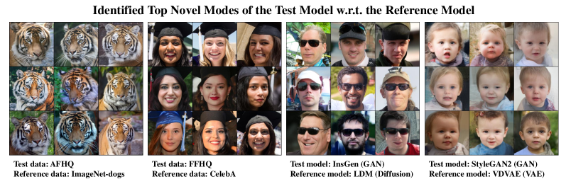
Figure 1: Our proposed entropy-based novelty can identify novel modes in real datasets and generative models.

Deep generative models including variational autoencoders (VAEs) [1], generative adversarial networks (GANs) [2], and denoising diffusion models [3] have attained remarkable results in many computer vision and speech processing settings. The success of these models is primarily due to the great capacity of deep neural networks to express the complex distributions of image and speech data. The impressive qualitative results of deep generative models have inspired many theoretical and empirical studies on their evaluation to reveal the advantages and disadvantages of existing architectures for training generative models.

To compare different generative modeling schemes, several evaluation metrics have been proposed in the literature. The existing evaluation scores for generative models can be classified into two main categories: 1) distance-based metrics such as the Fréchet inception distance (FID) [4] and kernel inception distance (KID) [5] measuring the closeness of the distribution of data and a generative model, 2) quality, diversity, and generalizability scores such as Inception score [6], precision/recall [7, 8], and density/coverage [9] scores assessing the sharpness and variety of the learned generative model. The mentioned metrics in these categories tend to assign higher scores to the models closer to the underlying data distribution. While such a property is desired in the performance evaluation of a learning framework, it may not result in an assessment of a generative model’s novelty compared to a baseline generative model or a particular reference distribution.

However, the recent developments of massive text-based and image-based generative models highlight the need to assess a model’s novelty and the uncommonness of its produced data in comparison to other generative models, because an interpretable comparison between different generative models requires the identification of missing sample types in one model that are present in other models’ generated data or a reference dataset. Importantly, massive text-to-image generative models are often utilized to create novel objects and scenes without targeting a specific data distribution, and therefore, an important criterion in their evaluation can be their expressed novelty with respect to a reference dataset.

In this work, we focus on the novelty evaluation task in the context of multi-modal distributions which are commonly present in large-scale image and text datasets due to the different background features of the collected data. Therefore, we suppose the test generative models consist of multiple modes and aim to identify and count the novel modes captured by one model which are more significantly expressed compared to a reference dataset. To this end, we propose a matrix-based entropic score which we call Kernel-based Entropic Novelty (KEN) to quantify the modes present in a test distribution $P$ with a higher frequency than in a reference distribution $Q$. Such a novelty quantification can be useful for comparing the modes captured by various generative models. Hence, the mode-based novelty evaluation can be used to debug and improve the training frameworks of generative models in application to multi-modal datasets.

Specifically, in our proposed framework, we focus on the eigenspace of the kernel covariance matrices of the test and reference distributions. We show that the principal eigenvectors of the kernel covariance matrix will approximate the mean barycenter of the major modes in a mixture distribution with well-separable components. Based on this interpretation, we analyze the eigenspectrum of the difference between the kernel covariance matrices corresponding to distributions $P$ and $Q$. We show the application of this eigendecomposition to identify the novel modes of $P$ with less frequency in $Q$. As a result, to quantify the mode-based novelty, we propose to compute the entropy of the positive eigenvalues of the difference covariance matrix, which we define to be the KEN score.

To compute the KEN score under high-dimensional kernel feature maps, e.g. the Gaussian kernel with an infinite-dimensional feature map, we develop a kernel-based method to compute the matrix’s eigenvalues and eigenvectors. The proposed algorithm only requires the knowledge of pairwise kernel similarity scores between the observed $\mathbf{X}$ and $\mathbf{Y}$ samples and circumvents the computation challenges under high-dimensional kernel feature maps. Also, while the original matrix-based approach leads to the computation of eigenvalues for a non-Hermitian matrix, we demonstrate the application of the Cholesky decomposition method to reduce the problem to an eigendecomposition of a symmetric matrix, which can be handled more efficiently by standard linear algebra programming packages.

Finally, we present the numerical application of our proposed methodology to several synthetic and real image datasets. For the synthetic experiments, we apply the novelty quantification method to multiple settings with Gaussian mixture models and show the method can successfully count and detect the additional modes in the test distribution compared to a reference mixture model. In our experiments on real datasets, we show the application of the method for identifying the different expressed modes between standard image datasets such as CelebA, AFHQ, FFHQ, and ImageNet. The numerical results show the methods’ success in detecting the novel concepts present in the datasets which could help enrich the datasets with samples from the detected less-expressed types. Furthermore, we apply the method to find the modes expressed with different frequencies by state-of-the-art generative modeling frameworks. The following is a summary of this work’s main contributions:

• Proposing a kernel-based spectral method to quantify mode-based novelty across multi-modal distributions,

• Interpreting the novelty quantification method with theoretical results on sub-Gaussian mixture models,

• Developing a method using the kernel trick for computing the mode-based novelty score under kernels with potentially infinite-dimensional feature maps,

• Applying the proposed method to detect different modes between standard generative models and datasets.

2 Related Work

Fidelity and diversity evaluation of generative models. The evaluation of generative models has been studied in a large body of related works as surveyed in [10]. The literature has proposed several metrics for the evaluation of the model’s distance to the data distribution [4, 5], quality, and diversity [6, 7, 8, 9, 11]. Except [11], these works do not focus on mixture distributions. Also, our analysis concerns a novelty evaluation between two distributions, different from the diversity assessment method proposed by Jalali et al. [11].
Generalization evaluation of generative models. Several related works aim to measure the generalizability of generative models from training to test data. Alaa et al. [12] use the percentage of authenticity to measure the likelihood of generated data copying the training data. Meehan et al. [13] analyze training data-copying tendency by comparing the average distance to the closest training and test samples. Jiralerspong et al. [14] examine overfitting by comparing the likelihoods based on training and test set. We note that the novelty evaluation task considered in our work is different from the generalizability assessment performed in these works, because our definition of mode-based novelty puts more emphasis on out-of-distribution modes not existing in the reference dataset. Also, we note that the reference dataset in out analysis may not be the training set of generative models, resulting in a different task from a training-to-test generalization evaluation.
Sample rarity and likelihood divergence. Han et al. [15] empirically show that rare samples are far from the reference data in the feature space. They propose the rarity score as the nearest-neighbor distance to measure the uncommonness of image samples. Also, Jiralerspong et al. [14] measure the difference in the likelihood of generated distribution to the training and another reference dataset. They propose measuring the likelihood divergence and interpreting novelty as low memorization of training samples. We note that both these evaluations lead to sample-based scores aiming to measure the uncommonness of a single data point. On the other hand, our proposed novelty evaluation is a distribution-based evaluation where we aim to measure the overall mode-based novelty of a model compared to a reference distribution.

3 Preliminaries

3.1 Novelty Evaluation of Generative Models

Consider a generator function $G:\mathbb{R}^{r}\rightarrow\mathbb{R}^{d}$ mapping an $r$-dimensional latent vector $\mathbf{Z}$ to $G(\mathbf{Z})$ which is aimed to be a real-like sample mimicking the data distribution $P_{\text{\rm data}}$. Here $\mathbf{Z}$ is drawn according to a known distribution, e.g. an isotropic Gaussian $\mathcal{N}(\mathbf{0},\sigma^{2}I)$. However, the probability distribution of random vector $G(\mathbf{Z})$ could be challenging to compute for a neural network $G$. The goal in the evaluation of generative model $P_{G(\mathbf{Z})}$ is to quantify and estimate a desired property of its generated samples, e.g. quality and diversity, from $n$ independently generated samples $G(\mathbf{z}_{1}),\ldots,G(\mathbf{z}_{n})$.

In this work, we focus on the evaluation of novelty in the generated data compared to a reference distribution $Q$ for a random $d$-dimensional vector $\mathbf{Y}$. We assume we have access to $m$ samples in $\{\mathbf{y}_{1},\ldots,\mathbf{y}_{m}\}$ drawn independently from $Q$. Also, for brevity, we denote the generative model $G$’s generated data by $\mathbf{x}_{i}=G(\mathbf{z}_{i})$ for every $1\leq i\leq n$. Therefore, our aim is to quantify the novelty of generated dataset $\{\mathbf{x}_{1},\ldots,\mathbf{x}_{n}\}$ compared to reference dataset $\{\mathbf{y}_{1},\ldots,\mathbf{y}_{m}\}$.

A central assumption in our theoretical analysis is that the test (generated) samples come from a multi-modal distribution. We use $P=\sum_{i=1}^{k}\omega_{i}P_{i}$ to represent a $k$-modal mixture distribution where every component $P_{i}$ has frequency $\omega_{i}$. Note that $[\omega_{1},\ldots,\omega_{k}]$ represent a probability model on the $k$ modes in $P$ satisfying $\omega_{i}\geq 0$ for every $i$ and $\sum_{i=1}^{k}\omega_{i}=1$. In our theoretical analysis, we assume sub-Gaussian components in $P$, i.e., every $P_{i}$ is a sub-Gaussian distribution with parameter $\boldsymbol{\sigma}^{2}_{i}$. The sub-Gaussian definition implies that given the mean vector $\boldsymbol{\mu}_{i}$ the moment-generating function (MGF) of $P_{i}$ satisfies the following inequality for every vector $\boldsymbol{\alpha}\in\mathbb{R}^{d}$:

$$\mathbb{E}_{\mathbf{X}\sim P_{i}}\Bigl{[}\exp\bigl{(}\boldsymbol{\alpha}^{\top}(\mathbf{X}-\boldsymbol{\mu}_{i})\bigr{)}\Bigr{]}\,\leq\,\exp\Bigl{(}\frac{\sigma_{i}^{2}\|\boldsymbol{\alpha}\|_{2}^{2}}{2}\Bigr{)}.$$

Notably, the above assumption holds not only under a Gaussian $\mathcal{N}(\boldsymbol{\mu}_{i},\Sigma_{i})$ with $\Sigma_{i}\preceq\sigma_{i}^{2}I$ , but further under any norm-bounded random vector satisfying $\|\mathbf{X}-\boldsymbol{\mu}_{i}\|_{2}\leq\sigma_{i}$.

3.2 Kernel Function and Kernel Covariance Matrix

Consider a kernel function $k:\mathbb{R}^{d}\times\mathbb{R}^{d}\rightarrow\mathbb{R}$ mapping every two vectors $\mathbf{x},\mathbf{y}\in\mathbb{R}^{d}$ to a similarity score $k(\mathbf{x},\mathbf{y})$ satisfying the positive semi-definite (PSD) property, i.e. the kernel matrix $K=\bigl{[}k(\mathbf{x}_{i},\mathbf{x}_{j})\bigr{]}_{n\times n}$ is a symmteric PSD matrix for every selection of input vectors $\mathbf{x}_{1},\ldots,\mathbf{x}_{n}$. In this paper, we commonly suppose a normalized Gaussian kernel $k_{G(\sigma)}$ with bandwidth parameter $\sigma$ defined as

$$k_{G(\sigma)}\bigl{(}\mathbf{x},\mathbf{y}\bigr{)}\,:=\,\exp\Bigl{(}\frac{-\|\mathbf{x}-\mathbf{y}\|^{2}_{2}}{2\sigma^{2}}\Bigr{)}.$$

Note that we call a kernel function $k$ normalized if for every $\mathbf{x}$ we have $k(\mathbf{x},\mathbf{x})=1$. We remark that the PSD property of a kernel function $k$ is equivalent to the existence of a feature map $\phi:\mathbb{R}^{d}\rightarrow\mathbb{R}^{s}$ such that for every input vectors $\mathbf{x,y}$ we have $k\bigl{(}\mathbf{x},\mathbf{y}\bigr{)}=\bigl{\langle}\phi(\mathbf{x}),\phi(\mathbf{y})\bigr{\rangle}$, where $\langle\cdot,\cdot\rangle$ denotes the inner product in $\mathbb{R}^{s}$.

Given a distribution $P$ with probability density function $p(\mathbf{x})$ on $\mathbf{X}\in\mathbb{R}^{d}$, we define the kernel covariance matrix according to kernel $k$ with feature map $\phi$ as

$$C_{\mathbf{X}}\,:= \,\mathbb{E}_{\mathbf{X}\sim P}\bigl{[}\phi(\mathbf{X})\phi(\mathbf{X})^{\top}\bigr{]}\,=\,\int p(\mathbf{x})\phi(\mathbf{x})\phi(\mathbf{x})^{\top}\mathrm{d}\mathbf{x}.$$

Using the empirical distribution $\widehat{P}_{n}$ of $n$ samples $\mathbf{x}_{1},\ldots,\mathbf{x}_{n}$ the kernel covariance matrix will be

$$\widehat{C}_{\mathbf{X}}=\frac{1}{n}\sum_{i=1}^{n}\phi(\mathbf{x}_{i})\phi(\mathbf{x}_{i})^{\top},$$

which can be written as $\widehat{C}_{\mathbf{X}}=\frac{1}{n}\Phi_{\mathbf{X}}\Phi_{\mathbf{X}}^{\top}$ that $\Phi_{\mathbf{X}}$ is an $n\times s$ matrix with every $i$-th row being $\phi(\mathbf{x}_{i})$.

Proposition 1.

Using the above definitions, $\widehat{C}_{\mathbf{X}}$ shares the same eigenvalues with the $n\times n$ normalized kernel matrix $\frac{1}{n}\bigl{[}k(\mathbf{x}_{i},\mathbf{x}_{j})\bigr{]}_{n\times n}$ with every $(i,j)$th entry being $\frac{1}{n}k(\mathbf{x}_{i},\mathbf{x}_{j})$. Therefore, assuming a normalized kernel function, the eigenvalues of $\widehat{C}_{\mathbf{X}}$ are non-negative and sum up to $1$.

4 A Spectral Approach to Novelty Evaluation for Mixture Models

In this section, we propose a spectral approach to the novelty evaluation of a generated $\mathbf{X}$ with mixture distribution $P=\sum_{i=1}^{k}\omega_{i}P_{i}$ in comparison to a reference $\mathbf{Y}$ distributed according to mixture model $Q=\sum_{i=1}^{t}\gamma_{i}Q_{i}$. In what follows, we first define and intuitively explain the proposed novelty evaluation score. We also discuss how to reduce the score computation task to the analysis of a kernel matrix. Next sections, we will provide a theoretical analysis of the framework in a setting where the mixture models consist of well-separable sub-Gaussian components, and present proofs for our kernel-based algorithm to compute the novelty score.

To define the proposed novelty score, we focus on the kernel covariance matrices of $\mathbf{X}$ and $\mathbf{Y}$, denoted by $C_{\mathbf{X}}$ and $C_{\mathbf{Y}}$, respectively. We will show in this section that under a Gaussian kernel with proper bandwidth, $C_{\mathbf{X}}$ and $C_{\mathbf{Y}}$ will contain the information of the modes in their eigendecomposition where the eigenvalues can be interpreted as the mode frequencies. Here, given a parameter $\eta\geq 1$, we define the $\eta$-conditional kernel covariance matrix $\Lambda_{\mathbf{X}|\eta\mathbf{Y}}$ as follows:

$$\Lambda_{\mathbf{X}|\eta\mathbf{Y}}\,:=\,C_{\mathbf{X}}-\eta C_{\mathbf{Y}}.$$

Note that if the components $P_{1},\ldots,P_{r}$ are shared between $P$ and $Q$, they will get canceled in the calculation of $\Lambda_{\mathbf{X}|\eta\mathbf{Y}}$ and thus will not result in a positive eigenvalue in the eigendecomposition of $\Lambda_{\mathbf{X}|\eta\mathbf{Y}}$ unless their frequency in $P$ is greater than $\eta$-times their frequency in $Q$. This shows how we can, loosely speaking, “subtract $Q$ from $P$” by subtracting their kernel covariance matrices in the above definition. Here, the hyperparameter $\eta\geq 1$ controls how much more frequent a mode in $P$ must be compared to the corresponding mode in $Q$ in order to be taken into account.

Therefore, we use the positive eigenvalues of $\Lambda_{\mathbf{X}|\eta\mathbf{Y}}$ to approximate the relative frequencies of the modes of $P$ that are expressed at least $\eta$-times more frequently than in $Q$. This allows us to define the following entropic score to quantify the novelty of $\mathbf{X}$ with respect to $\mathbf{Y}$.

Definition 1.

Consider the positive eigenvalues $\lambda_{1},\ldots,\lambda_{k^{\prime}}>0$ of $\Lambda_{\mathbf{X}|\eta\mathbf{Y}}=C_{\mathbf{X}}-\eta C_{\mathbf{Y}}$ and let $S=\sum_{i=1}^{k^{\prime}}\lambda_{i}$. The Kernel Entropic Novelty (KEN) score is

$$\text{\rm KEN}_{\eta}(\mathbf{X}|\mathbf{Y})\>:=\>\sum_{i=1}^{k^{\prime}}\lambda_{i}\log\frac{S}{\lambda_{i}}.$$

Intuitively, $\lambda_{i}/S$ is the relative frequency of the $i$-th novel mode in $P$, and the entropy of the novel mode distribution is $\sum_{i}(\lambda_{i}/S)\log(S/\lambda_{i})$. The entropy is multiplied by $S$ in the definition of $\text{\rm KEN}_{\eta}(\mathbf{X}|\mathbf{Y})$ for two reasons. First, the amount of novelty should not only increase with the entropy (or diversity) of the novel modes, but also increase with the total frequency $S$ of those modes. Second, this allows us to interpret $\text{\rm KEN}_{\eta}(\mathbf{X}|\mathbf{Y})$ as the conditional entropy of the information of the mode of $\mathbf{X}$ given the dataset of $\mathbf{Y}$.

To compute the KEN score, from observed data, in Section 6 we show that the non-zero eigenvalues of the conditional covariance matrix $\Lambda_{\mathbf{X}|\eta\mathbf{Y}}$ are the same as the following kernel-based matrix, which we call the $\eta$-conditional kernel matrix $K_{\mathbf{X}|\eta Y}$:

$$K_{\mathbf{X}|\eta\mathbf{Y}}\;=\;\begin{bmatrix}K_{\mathbf{X}\mathbf{X}}\hskip 5.69054pt&\sqrt{\eta}\,K_{\mathbf{X}\mathbf{Y}}\hskip 5.69054pt\vspace{3mm}\\ -\sqrt{\eta}\,K^{\top}_{\mathbf{X}\mathbf{Y}}\hskip 5.69054pt&-\eta\,K_{\mathbf{Y}\mathbf{Y}}\hskip 5.69054pt\vspace{1mm}\end{bmatrix}$$

Here, $K_{\mathbf{X}\mathbf{X}}=\frac{1}{n}\bigl{[}k(\mathbf{x}_{i},\mathbf{x}_{j})\bigr{]}_{n\times n}$ is defined as the normalized kernel matrix of samples $\mathbf{x}_{1},\ldots,\mathbf{x}_{n}$ from the test distribution, and similarly $K_{\mathbf{Y}\mathbf{Y}}=\frac{1}{m}\bigl{[}k(\mathbf{y}_{i},\mathbf{y}_{j})\bigr{]}_{m\times m}$ denotes the normalized kernel matrix of samples $\mathbf{y}_{1},\ldots,\mathbf{y}_{m}$ from the reference distribution. Also, $K_{\mathbf{X}\mathbf{Y}}=\frac{1}{\sqrt{nm}}\bigl{[}k(\mathbf{x}_{i},\mathbf{y}_{j})\bigr{]}_{n\times m}$ is the normalized cross-kernel matrix for the test and reference samples. Therefore, given observed samples from the test $P_{X}$ and reference $P_{Y}$ distributions, we propose to compute the positive eigenvalues $\lambda_{1},\ldots,\lambda_{r}>0$ of $K_{\mathbf{X}|\eta Y}$ and compute the KEN score using Definition 1. In addition, the eigenvectors $\mathbf{u}_{1},\ldots,\mathbf{u}_{r}\in\mathbb{R}^{n+m}$ corresponding to the positive eigenvalues will highlight the samples belonging to the identified $r$ novel modes.

5 Theoretical Analysis of the Spectral Novelty Evaluation

To theoretically analyze the proposed spectral method, we first focus on a single distribution $P$ with well-separable modes and show a relationship between the modes of $P$ and the eigendecomposition of its kernel covariance matrix.

Theorem 1.

Suppose that every component $P_{i}$ of a mixture distribution $P=\sum_{i=1}^{k}\omega_{i}P_{i}$ represents a sub-Gaussian distribution with mean vector $\boldsymbol{\mu}_{i}$ and sub-Gaussian parameter $\sigma_{i}^{2}$. Assume that $\omega_{1}\geq\omega_{2}\geq\cdots\geq\omega_{k}$ are sorted in a descending order. Then, the top $k$ eigenvalues $\lambda_{1}\geq\cdots\geq\lambda_{k}$ of the kernel covariance matrix $C_{\mathbf{X}}$ according to a Gaussian kernel with bandwidth $\sigma$ will satisfy:

$$\sum_{i=1}^{k}\bigl{(}\lambda_{i}-\omega_{i}\bigr{)}^{2}\;\leq\;4\sum_{i=1}^{k}\omega_{i}\Bigl{(}1-\frac{1}{\sqrt{\bigl{(}1+{2\sigma^{2}_{i}}/{\sigma^{2}}\bigr{)}^{d}}}\Bigr{)}+8\sum_{i=2}^{k}\sum_{j=1}^{i-1}\omega_{i}\exp\Bigl{(}\frac{-\|\boldsymbol{\mu}_{i}-\boldsymbol{\mu}_{j}\|^{2}_{2}}{\sigma^{2}}\Bigr{)}.$$

Proof.

We defer the proof to the Appendix. ∎

The above theorem shows that if the modes of the mixture distribution are well-separable, meaning that $\min_{1\leq i\neq j\leq k}\frac{\|\boldsymbol{\mu_{i}}-\boldsymbol{\mu_{j}}\|_{2}^{2}}{\sigma^{2}}\gg 1$ while the sub-Gaussian parameter of the components satisfy $\frac{\sigma_{i}^{2}}{\sigma^{2}}\ll 1$, then the eigendecomposition of the Gaussian kernel covariance matrix can discover the mode centers via the principal eigenvectors and the mode frequencies via the principal eigenvalues.

Given the interpretation provided by Theorem 1, the positive eigenvalues of $\Lambda_{\mathbf{X}|\eta\mathbf{Y}}=C_{\mathbf{X}}-\eta C_{\mathbf{Y}}$ will correspond to the modes of $\mathbf{X}$ that have a frequency at least $\eta$ times higher than the frequency of that mode in $\mathbf{Y}$. Therefore, the positive eigenvalues of $\Lambda_{\mathbf{X}|\eta\mathbf{Y}}$ can quantify and interpret the mode-based novelty of $\mathbf{X}$ with respect to $\mathbf{Y}$. The following theorem formalizes this intuition and shows how $\Lambda_{\mathbf{X}|\eta\mathbf{Y}}$’s positive eigenvalues explain the novelty of $\mathbf{X}$’s modes.

Theorem 2.

Consider multi-modal random vectors $\mathbf{X}\sim\sum_{i=1}^{k}\omega_{i}P_{i}$ and $\mathbf{Y}\sim\sum_{i=1}^{k}\gamma_{i}Q_{i}$, where $\omega_{1}-\eta\gamma_{1}\geq\cdots\geq\omega_{k}-\eta\gamma_{k}$. Suppose the corresponding mode to every sub-Gaussian $P_{i}$ with mean $\boldsymbol{\mu}_{i}$ is $Q_{i}$ with mean $\boldsymbol{\mu}^{\prime}_{i}=\boldsymbol{\mu}_{i}+\boldsymbol{\delta}_{i}$. Then, assuming that for every $i$, both $Q_{i}$ and $P_{i}$ are $\sigma_{i}^{2}$-sub-Gaussian, the positive eigenvalues $\lambda_{1}\geq\ldots\geq\lambda_{k^{\prime}}>0$ of $\Lambda_{\mathbf{X}|\eta\mathbf{Y}}$ satisfy (letting $\lambda_{i}=0$ if $i>k^{\prime}$)

$$\sum_{i=1}^{k}\Bigl{(}\lambda_{i}-\max\bigl{\{}\omega_{i}-\eta\gamma_{i},0\bigr{\}}\Bigr{)}^{2}\>\leq\> 8\sum_{i=1}^{k}\Bigl{[}(\omega_{i}+\eta^{2}\eta_{i})\Bigl{(}1-\frac{\exp\bigl{(}-2\|\boldsymbol{\delta}_{i}\|_{2}^{2}/{\sigma^{2}}\bigr{)}}{\sqrt{\bigl{(}1+{4\sigma^{2}_{i}}/{\sigma^{2}}\bigr{)}^{d}}}\Bigr{)}\Bigr{]}$$

$$\>+4(1+\eta)\sum_{i=2}^{k}\sum_{j=1}^{i-1}(\omega_{i}+\eta\gamma_{i})\exp\Bigl{(}\frac{-\|\boldsymbol{\mu}^{\prime}_{i}-\boldsymbol{\mu}^{\prime}_{j}\|^{2}_{2}}{\sigma^{2}}\Bigr{)}.$$

Proof.

We defer the proof to the Appendix. ∎

Based on the above theorem, the principal positive eigenvalues of the defined matrix $\Lambda_{\mathbf{X}|\eta\mathbf{Y}}$ show the extra frequencies of the modes with a more dominant presence in $\mathbf{X}$. As we increase the value of $\eta$, we require a stronger presence of $\mathbf{X}$’s modes to count them as a novel mode. In the limit case where $\eta\rightarrow+\infty$, we require a complete absence of an $\mathbf{X}$’s mode in $\mathbf{Y}$ to call it novel.

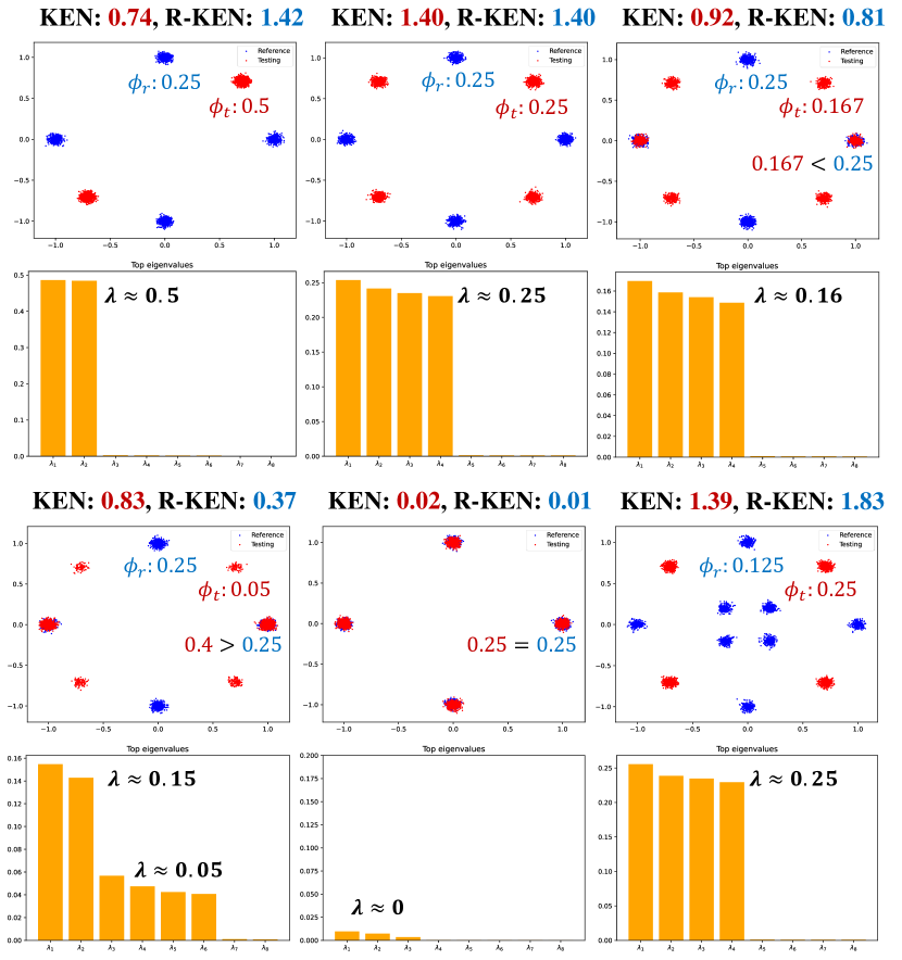
Figure 2: Experimental results on synthetic Gaussian mixture distributions including KEN and R-KEN (Reversed-KEN) scores, and principal eigenvalues of the conditional kernel covariance matrix $\Lambda_{\mathbf{X}|\eta\mathbf{Y}}$. Row 1 and 3: Reference (in blue) and test (in red) samples with $\phi_{t},\,\phi_{r}$ denoting the test and reference modes’ frequency. Row 2 and 4: Positive eigenvalues of conditional $\Lambda_{\mathbf{X}|\eta\mathbf{Y}}$.

Finally, note that $\mathrm{KEN}_{\eta}(\mathbf{X}|\mathbf{Y})$ can be interpreted as the conditional entropy of the information of the mode of $\mathbf{X}$ given the dataset of $\mathbf{Y}$. More precisely, if $\eta=1$ this score is the conditional entropy $H(X_{\mathrm{mode}}|Y_{\mathrm{adv}})$, where $X_{\mathrm{mode}}\in\{1,\ldots,k\}$ is the mode cluster variable of $\mathbf{X}$ (the index of the mode $\mathbf{X}$ belongs to), and $Y_{\mathrm{adv}}$ represents the knowledge of an adversary who knows the dataset of $\mathbf{Y}$ and wants to predict $X_{\mathrm{mode}}$. If the random sample $\mathbf{X}$ is also found in the dataset of $\mathbf{Y}$, then the adversary will know the mode of $\mathbf{X}$ and predicts $Y_{\mathrm{adv}}=X_{\mathrm{mode}}$ accurately; otherwise the adversary knows nothing about $X_{\mathrm{mode}}$, and outputs $Y_{\mathrm{adv}}=e$ as an erasure symbol denoting the lack of information.

Under the setting in Theorem 2 for $\eta=1$, $\lambda_{i}=\max\{\omega_{i}-\gamma_{i},0\}$, take $\mathbb{P}(Y_{\mathrm{adv}}\!=\!i|X_{\mathrm{mode}}\!=\!i)=\min\{\gamma_{i}/\omega_{i},1\}$ (otherwise $Y_{\mathrm{adv}}=e$) since among the samples of $\mathbf{X}$ with mode $i$, at most a portion $\gamma_{i}/\omega_{i}$ are also samples of $\mathbf{Y}$ (if sizes of the two datasets are equal). We have $\mathbb{P}(Y_{\mathrm{adv}}=e)=\sum_{i=1}^{k^{\prime}}\omega_{i}\max\{1-\gamma_{i}/\omega_{i},\,0\}=S$. Since $H(X_{\mathrm{mode}}|Y_{\mathrm{adv}}=i)=0$, we have

$$H(X_{\mathrm{mode}}|Y_{\mathrm{adv}}) =\mathbb{P}(Y_{\mathrm{adv}}=e)H(X_{\mathrm{mode}}|Y_{\mathrm{adv}}=e)$$

$$\;\;\;+\sum_{i=1}^{k}{\mathbb{P}(Y_{\mathrm{adv}}=i)H(X_{\mathrm{mode}}|Y_{\mathrm{adv}}=i)}$$

$$=S\times H(X_{\mathrm{mode}}|Y_{\mathrm{adv}}=e)$$

$$=S\sum_{i=1}^{k^{\prime}}\frac{\lambda_{i}}{S}\log\frac{S}{\lambda_{i}}\;=\;\mathrm{KEN}_{1}(\mathbf{X}|\mathbf{Y}).$$

For a general $\eta$, $\mathrm{KEN}_{\eta}(\mathbf{X}|\mathbf{Y})$ can be interpreted as $H(X_{\mathrm{mode}}|Y_{\mathrm{adv}})$ if each sample of $\mathbf{Y}$ allows the adversary to learn $\eta$ samples of $\mathbf{X}$ belonging to the same mode as $\mathbf{Y}$, resulting in $\mathbb{P}(Y_{\mathrm{adv}}=i\,|\,X_{\mathrm{mode}}=i)=\min\{\eta\gamma_{i}/\omega_{i},\,1\}$. The next section shows how we can use the kernel trick to compute the KEN score from the pairwise similarity scores between the observed test and reference samples.

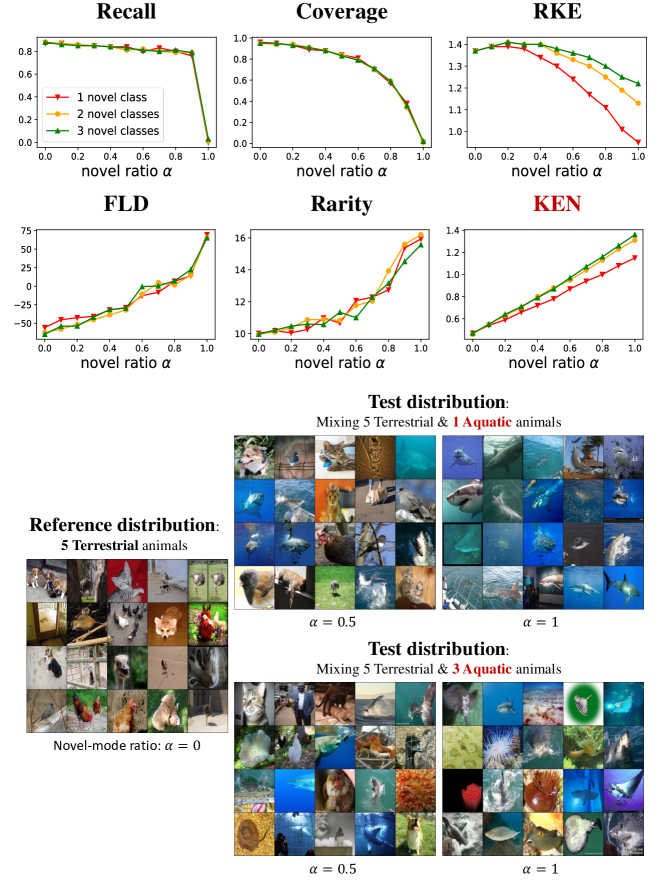
Figure 3: Top: Trends of baseline and KEN scores in evaluating novel yet less-diverse distributions. Bottom: ImageNet-1K Samples from reference and test distributions. Reference modes: 5 terrestrial animals. Novel modes: 1-3 aquatic lives. $\alpha$ is the ratio of novel modes in testing distribution. $\alpha=0,1$ represents pure reference and novel distributions, respectively.

6 Computation of the KEN Novelty Score

Since the KEN score is characterized using the difference $C_{\mathbf{X}}-\eta C_{\mathbf{Y}}$ of kernel covariance matrices, the computation of this score will be challenging in the kernel feature space under a high-dimensional kernel feature map. Specifically, the kernel feature map for a Gaussian kernel is infinitely high-dimensional. Our next theorem reduces the eigendecomposition task to the analysis of kernel similarity scores of observed samples.

Theorem 3.

Suppose we observed empirical samples $\mathbf{x}_{1},\ldots,\mathbf{x}_{n}$ from test distribution $P$ and $\mathbf{y}_{1},\ldots,\mathbf{y}_{m}$ from reference distribution $Q$. Then, the difference of empirical kernel covariance matrices $\widehat{\Lambda}_{\mathbf{X}|\eta\mathbf{Y}}=\widehat{C}_{\mathbf{X}}-\eta\widehat{C}_{\mathbf{Y}}$ shares the same positive eigenvalues with the following block matrix:

$$K_{\mathbf{X}|\eta\mathbf{Y}}\>:=\>\begin{bmatrix}K_{\mathbf{X}\mathbf{X}}\hskip 4.2679pt&\sqrt{\eta}\,K_{\mathbf{X}\mathbf{Y}}\hskip 4.2679pt\vspace{3mm}\\ -\sqrt{\eta}\,K^{\top}_{\mathbf{X}\mathbf{Y}}\hskip 4.2679pt&-\eta\,K_{\mathbf{Y}\mathbf{Y}}\hskip 4.2679pt\vspace{1mm}\end{bmatrix}$$

In the above, $K_{\mathbf{X}\mathbf{X}}=\frac{1}{n}\bigl{[}k(\mathbf{x}_{i},\mathbf{x}_{j})\bigr{]}_{n\times n}$ and $K_{\mathbf{Y}\mathbf{Y}}=\frac{1}{m}\bigl{[}k(\mathbf{y}_{i},\mathbf{y}_{j})\bigr{]}_{m\times m}$ are the kernel similarity matrices for observed $\mathbf{X}$ and $\mathbf{Y}$, samples respectively, and $K_{\mathbf{X}\mathbf{Y}}=\frac{1}{\sqrt{nm}}\bigl{[}k(\mathbf{x}_{i},\mathbf{y}_{j})\bigr{]}_{n\times m}$ is the $n\times m$ cross-kernel matrix between observed ${\mathbf{X},\mathbf{Y}}$ samples.

Proof.

We defer the proof to the Appendix. ∎

Theorem 3 simplifies the eigendecomposition of the matrix $\widehat{\Lambda}_{\mathbf{X}|\eta\mathbf{Y}}$ to the $(n+m)\times(n+m)$ kernel-based matrix $K_{\mathbf{X}|\eta\mathbf{Y}}$. While this task can be addressed via $O((n+m)^{3})$ computations, the derived $K_{\mathbf{X}|\eta\mathbf{Y}}$ is a non-Hermitian matrix for which the standard Hermitian matrix-based algorithms do not apply. In the following theorem, we show the application of Cholesky decomposition to reduce the task to an eigenvalue computation for a symmetric matrix.

Theorem 4.

In the setting of Theorem 3, define the following joint kernel matrix:

$$K_{\mathbf{X},\eta\mathbf{Y}}\>:=\>\begin{bmatrix}K_{\mathbf{X}\mathbf{X}}\hskip 4.2679pt&\sqrt{\eta}\,K_{\mathbf{X}\mathbf{Y}}\hskip 4.2679pt\vspace{2mm}\\ \sqrt{\eta}\,K^{\top}_{\mathbf{X}\mathbf{Y}}\hskip 4.2679pt&\eta\,K_{\mathbf{Y}\mathbf{Y}}\hskip 4.2679pt\vspace{2mm}\end{bmatrix}$$

Consider the Cholesky decomposition of the above PSD matrix satisfying $K_{\mathbf{X},\eta\mathbf{Y}}=V^{\top}V$ for upper-triangular matrix $V\in\mathbb{R}^{(m+n)\times(m+n)}$. Then, $\widehat{\Lambda}_{\mathbf{X}|\eta\mathbf{Y}}$ shares the same non-zero eigenvalues with the symmetric matrix $VDV^{\top}$ where $D$ is a $(m+n)\times(m+n)$ diagonal matrix with diagonal entries in $\bigl{[}\underbrace{+1,\ldots,+1}_{\text{\rm n times}},\underbrace{-1,\ldots,-1}_{\text{\rm m times}}\bigr{]}$.

Proof.

We defer the proof to the Appendix. ∎

Based on the above theorem, we propose Algorithm 1 to compute the KEN score and find the eigendirections corresponding to the detected novel modes. We note that the eigendecomposition task in the algorithm reduces to the spectral decomposition of a symmetric matrix that can be handled more efficiently than the eigenvalue computation for a general non-symmetric matrix.

Algorithm 1 Computation of KEN & novel mode centers

1:Input: Sample sets $\{\mathbf{x}_{1},\ldots,\mathbf{x}_{n}\}$ and $\{\mathbf{y}_{1},\ldots,\mathbf{y}_{m}\}$, parameter $\eta>0$, Gaussian kernel bandwidth $\sigma$

2:Compute matrices $K_{\mathbf{X}\mathbf{X}}=\frac{1}{n}[k(\mathbf{x}_{i},\mathbf{x}_{j})]_{n\times n}$, $K_{\mathbf{Y}\mathbf{Y}}=\frac{1}{m}[k(\mathbf{y}_{i},\mathbf{y}_{j})]_{m\times m}$, $K_{\mathbf{X}\mathbf{Y}}=\frac{1}{\sqrt{mn}}[k(\mathbf{x}_{i},\mathbf{y}_{j})]_{n\times m}$

3:Apply Cholesky decomposition to compute upper-triangular $V\in\mathbb{R}^{\tiny(n+m)\times(n+m)}$ such that

$$V^{\top}V\,=\,\begin{bmatrix}K_{\mathbf{X}\mathbf{X}}&\sqrt{\eta}\,K_{\mathbf{X}\mathbf{Y}}\vspace{1mm}\\ \sqrt{\eta}\,K^{\top}_{\mathbf{X}\mathbf{Y}}&\eta\,K_{\mathbf{Y}\mathbf{Y}}\end{bmatrix}$$

4:Compute $\Gamma=V\mathrm{diag}\{[\underbrace{+1,\ldots,+1}_{\text{\rm n times}},\underbrace{-1,\ldots,-1}_{\text{\rm m times}}]\}V^{\top}$

5:Perform eigendecomposition to get $\Gamma=U^{\top}\mathrm{diag}(\boldsymbol{\lambda})U$

6:Find the non-negative eigenvalues $\lambda_{1},\ldots,\lambda_{k}\geq 0$

7:Output: $\text{\rm KEN-score}=\sum_{i=1}^{k}\lambda_{i}\log\frac{\sum_{j=1}^{k}\lambda_{j}}{\lambda_{i}}$ and eigenvectors $\mathbf{u}_{1},\ldots,\mathbf{u}_{k}$.

7 Numerical Results

7.1 Experimental Setup

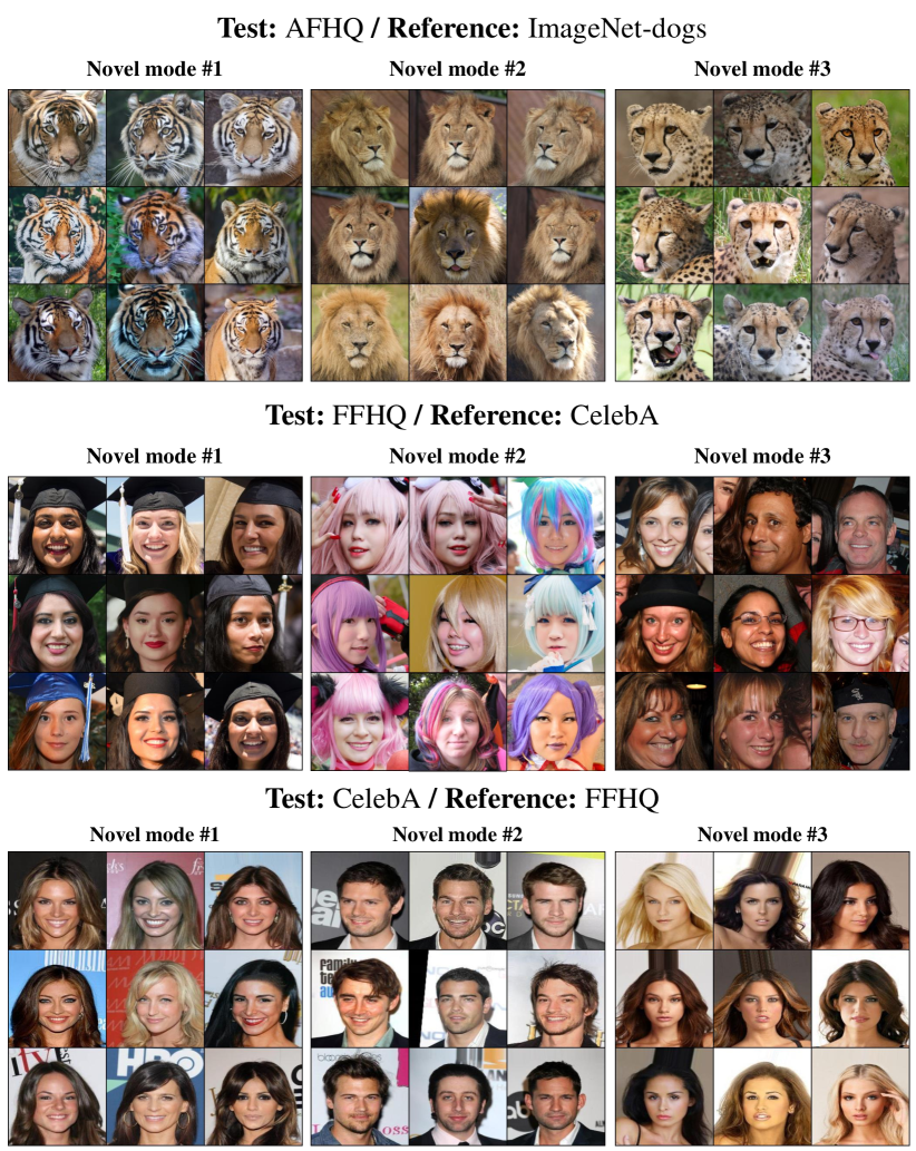
Figure 4: Identified top-3 novel modes between image datasets: (Top) AFHQ w.r.t. ImageNet-dogs, (Middle) FFHQ w.r.t. CelebA, (Bottom) CelebA w.r.t FFHQ.

Datasets. We performed experiments on the following image datasets: 1) CIFAR-10 [16] with 60k images of 10 classes, 2) ImageNet-1K [17] with 1.4 million images of 1000 classes, containing 20k dog images from 120 different dog breeds, 3) CelebA [18] with 200k face images of celebrities, 4) FFHQ [19] with 70k human-face images, 5) AFHQ [20] with 15k animal-face images of dogs, cats, and wildlife. The AFHQ-dog subset has 5k images from 8 dog breeds.
Pre-trained generative models and neural nets for feature extraction: We followed the standard in the literature to use a pre-trained Inception-V3 [21] to extract features. For a fair comparison between standard generative models, we downloaded all the pre-trained generator networks from the StudioGAN [22] repository.
Bandwidth parameter $\sigma$ and sample size: Similar to [11], we chose the kernel bandwidth to be the smallest $\sigma$ satisfying variance $<0.01$. In our experiments, we observed $\sigma\in[10,15]$ could satisfy this requirement for all the tested image data with Inception-V3-extracted features. In the case of synthetic Gaussian mixtures, we used $\sigma=0.5$. In our experiments, we used $m,n=5000$ sample size for the test and reference data.

7.2 Numerical Results on Synthetic Gaussian Mixtures

First, we tested the proposed methodology on Gaussian mixture models (GMMs) as shown in Figure 2. The experiments use the standard setting of 2-dimensional Gaussian mixtures in [23]. We show the samples from the reference distribution (in blue) with a 4-component GMM where the components are centered at [0, 1], [1, 0], [0, -1], [-1, 0]. The generated data in the test distribution (in red) follow a Gaussian mixture in all the experiments, where we center the novel modes (unexpressed in the reference) at [$\pm 0.7$, $\pm 0.7$] and center the shared modes at the same component-means of the reference distribution. In the experiments, we chose parameter $\eta=1$ for the KEN evaluation.

Based on the KEN scores and eigenspectrum of the $\eta$-conditional kernel matrix reported in Figure 2, our proposed spectral method successfully identifies the novel modes, and the KEN scores correlate with the novel modes’ number and frequencies. We highlight the following trends in the evaluated KEN scores:

1. More novel modes result in a greater KEN score. The first two columns of Figure 2 illustrate that adding two novel modes to the test distribution increases the KEN score from 0.74 to 1.40. The bar plots of the conditional kernel matrix’s eigenvalues also show two extra principal eigenvalues approximating the frequencies of novel modes.

2. Transferring weight from novel to common modes decreases the KEN score. Columns 3-5 in Figure 2 show the effects of overlapping modes on KEN score. In Column 3, the test distribution has six components with uniform frequencies of $1/6$, of which two modes are centered at the same points as the reference modes with frequency $1/4$. The KEN score decreased from 1.40 to 0.92, and we observed only four principal eigenvalues in the conditional kernel matrix. Also, when we increased the frequencies of the common modes from 0.25 to 0.4, as shown in Column 4, we could observe 6 outstanding eigenvalues, from which two of them approximate the difference of common mode frequencies. Moreover, under two identical distributions, the KEN score was nearly 0.

3. KEN does not behave symmetrically between the reference and test distributions. In our experiments, we also measured the KEN score of the reference distribution with respect to the test distribution, which we call Reverse KEN (R-KEN). We observed that the KEN and R-KEN scores could behave differently, and the roles of test and reference distributions were different. Regarding KEN and R-KEN’s mismatch, when we included four extra reference modes in the last column, the KEN score did not considerably change (1.40 vs. 1.39) while the R-KEN value jumped from 1.40 to 1.83.

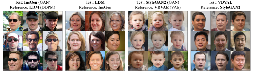
Figure 5: Identified top novel modes between FFHQ-trained generative models.

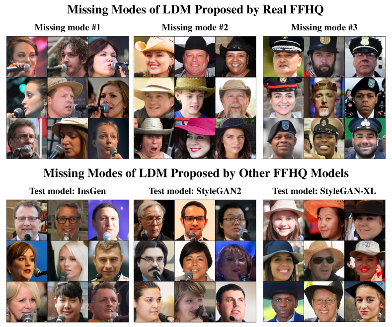
Figure 6: Missing modes of LDM in FFHQ. Training set and other generative models both capture similar missing modes of LDM with large $\eta=10$ in $K_{X|\eta Y}$.

7.3 Novelty vs. Diversity Evaluation via KEN and Baseline Metrics

The novelty and diversity evaluation criteria may not align under certain conditions. To test our proposed method and the existing scores’ capability to capture novelty under less diversity, we designed experimental settings where the test distribution possessed less diversity while containing novel modes compared to the reference distribution. The baseline diversity-based scores we attempted in the experiment were improved Recall [24], Coverage [9], and RKE [11]. We also evaluated the sample divergence: FLD [14] and sample Rarity [15], which are proposed to assess sample-based novelty. We extract images from 5 terrestrial animal classes in ImageNet-1K to form the reference distribution $P_{r}$ and images from 1-3 aquatic life classes to form the novel distribution $P_{n}$. To simulate different novelty ratios, we mixed the two distributions with a ratio parameter $0\leq\alpha\leq 1$ to form the test distribution as $P_{t}=\alpha P_{n}+(1-\alpha)P_{r}$.

As shown in Figure 3, all the diversity-based baseline metrics decreased under a larger $\alpha$, i.e., as the test distribution $P_{t}$ becomes closer to the novel distribution $P_{n}$. The observation can be interpreted as the diversity and novelty levels change in opposite directions in this experiment. The proposed KEN score and baseline FLD and Rarity scores could capture the higher novelty and increased with $\alpha$. On the other hand, when we increased the number of novel modes from 1 to 3 aquatic animals, the sample-based FLD and Rarity scores did not change significantly, while our proposed KEN score could capture the extra novel modes and grew with the number of novel modes. This experiment shows the distribution-based novelty evaluation by the KEN score vs. the sample-based novelty evaluation by FLD and Rarity.

Table 1: FFHQ-trained generative models’ pairwise KEN score

Generative Models (Test Models)	Reference Models
	InsGen	LDM	StyleGAN2	VDVAE	StyleGAN-XL	Avg. KEN
InsGen [25]	-	1.26	1.18	1.87	1.17	1.37
LDM [26]	1.09	-	1.14	1.59	1.08	1.23
StyleGAN2 [19]	1.12	1.26	-	1.76	1.18	1.33
VDVAE [27]	0.96	0.91	0.94	-	0.95	0.94
StyleGAN-XL [28]	1.16	1.24	1.19	1.83	-	1.36

7.4 Numerical Results on Real/Generated Image Data

We evaluated the KEN score and visualized identified novel modes for the real image dataset and sample sets generated by widely-used generative models. For the identification of samples belonging to the detected novel modes, we followed Algorithm 1 to obtain the eigenvectors corresponding to the top eigenvalues. Every eigenvector $\mathbf{u}_{i}$ is an $(m+n)$-dimensional vector where the entries (sample indices) with significant values greater than a threshold $\rho$ are clustered as mode $i$. In our visualization, we show top-$r$ images with the maximum entry value on the shown top eigenvectors as the top novel modes.

Novel modes between real datasets. Based on the proposed method, we visualized the novel modes samples across content-similar datasets (AFHQ, ImageNet-dogs) and (FFHQ, CelebA). Figure 4 visualizes the identified samples from the top-3 novel modes (principal eigenvectors). We observed that the detected modes are representing visually-meaningful picture types of animal types in the ImageNet-dogs case and the ”students wearing graduation caps”, ”individuals with distinct hair colors”, and ”double-individuals group photo”. We could not find such samples when searching for these image types in the reference datasets. We put the presentation of similar visualizations on other datasets to the Figure 9.

Novel modes between standard generative models. We analyzed FFHQ-trained models: GAN-based InsGen, StyleGAN2, StyleGAN-XL, diffusion-based LDM, and VAE-based VDVAE. Figure 5 illustrates samples from the detected top novel mode between different pairs of generative models. For example, we observed that InsGen has more novelty in ”people wearing sunglasses” than LDM, and StyleGAN2 has more novelty in ”kids” than VDVAE. We present and discuss more visualizations for other pairs of generative models in Figure 10. According to Table 1. considering the averaged KEN scores over all ${5\choose 2}$ pairs, InsGen obtained the maximum averaged-KEN among the tested generative models.

Detection of missing sample types of generative models. To detect missing modes of the generators, we used the larger value $\eta=10$ for parameter $\eta$ in the computation of $K_{\mathbf{X}|\eta\mathbf{Y}}$. For example, our experimental results suggest the sample types ”Microphone”, ”Round hat”, and ”Black uniform hat” to be not well-expressed in LDM. The visualization of our numerical results is presented in Figure 6. We also present the applications of our spectral method for conditionally generating novel-mode samples in Figure 8 and benchmarking model fitness in Table 2.

8 Conclusion

In this paper, we proposed a spectral method for the evaluation of the novel modes in a mixture distribution $P$ which are expressed more frequently than in a reference distribution $Q$. We defined the KEN score to measure the entropy of the novel modes and tested the evaluation method on benchmark synthetic and image datasets. We note that our numerical evaluation focused on computer vision settings, and its extension to language models will be an interesting future direction. Also, characterizing tight statistical and computational complexity bounds for the novelty evaluation method will be a related topic for future exploration.

Appendix A Proofs

A.1 Proof of Theorem 1

To prove the theorem, note that every mode variable $\mathbf{X}_{i}\sim P_{i}$ can be written as $\mathbf{X}_{i}=\boldsymbol{\mu}_{i}+\mathbf{V}_{i}$ where $\mathbf{V}_{i}$ is a zero-mean random vector satisfying the following sub-Gaussian property for every vector $\boldsymbol{\alpha}\in\mathbb{R}^{d}$:

$$\mathbb{E}\bigl{[}\exp\big{(}\boldsymbol{\alpha}^{\top}\mathbf{V}\big{)}\bigr{]}\leq\exp\Bigl{(}\frac{\sigma_{i}^{2}\|\boldsymbol{\alpha}\|^{2}_{2}}{2}\Bigr{)}.$$

Then, we can write the kernel covariance matrix $C_{\mathbf{X}}$ as

$$C_{\mathbf{X}}\,=\,\sum_{i=1}^{k}\Bigl{[}\omega_{i}\phi(\boldsymbol{\mu}_{i})\phi(\boldsymbol{\mu}_{i})^{\top}\Bigr{]}+\sum_{i=1}^{k}\Bigl{[}\omega_{i}\Bigr{(}\mathbb{E}\bigl{[}\phi(\boldsymbol{\mu}_{i}+\mathbf{V}_{i})\phi(\boldsymbol{\mu}_{i}+\mathbf{V}_{i})^{\top}\bigr{]}-\phi(\boldsymbol{\mu}_{i})\phi(\boldsymbol{\mu}_{i})^{\top}\Bigr{)}\Bigr{]}.$$

Therefore, we can write

$$\Bigl{\|}C_{\mathbf{X}}-\sum_{i=1}^{k}\omega_{i}\phi(\boldsymbol{\mu}_{i})\phi(\boldsymbol{\mu}_{i})^{\top}\Bigr{\|}^{2}_{F}=\, \Bigl{\|}\sum_{i=1}^{k}\biggl{[}\omega_{i}\Bigr{(}\mathbb{E}\bigl{[}\phi(\boldsymbol{\mu}_{i}+\mathbf{V}_{i})\phi(\boldsymbol{\mu}_{i}+\mathbf{V}_{i})^{\top}\bigr{]}-\phi(\boldsymbol{\mu}_{i})\phi(\boldsymbol{\mu}_{i})^{\top}\Bigr{)}\biggr{]}\Bigr{\|}^{2}_{F}$$

$$\stackrel{{\scriptstyle(a)}}{{\leq}}\, \sum_{i=1}^{k}\biggl{[}\omega_{i}\Bigl{\|}\mathbb{E}\bigl{[}\phi(\boldsymbol{\mu}_{i}+\mathbf{V}_{i})\phi(\boldsymbol{\mu}_{i}+\mathbf{V}_{i})^{\top}\bigr{]}-\phi(\boldsymbol{\mu}_{i})\phi(\boldsymbol{\mu}_{i})^{\top}\Bigr{\|}^{2}_{F}\biggr{]}$$

$$=\, \sum_{i=1}^{k}\biggl{[}\omega_{i}\Bigl{\|}\mathbb{E}\bigl{[}\phi(\boldsymbol{\mu}_{i}+\mathbf{V}_{i})\phi(\boldsymbol{\mu}_{i}+\mathbf{V}_{i})^{\top}-\phi(\boldsymbol{\mu}_{i})\phi(\boldsymbol{\mu}_{i})^{\top}\bigr{]}\Bigr{\|}^{2}_{F}\biggr{]}$$

$$\stackrel{{\scriptstyle(b)}}{{\leq}}\, \sum_{i=1}^{k}\omega_{i}\mathbb{E}\Bigl{[}\Bigl{\|}\phi(\boldsymbol{\mu}_{i}+\mathbf{V}_{i})\phi(\boldsymbol{\mu}_{i}+\mathbf{V}_{i})^{\top}-\phi(\boldsymbol{\mu}_{i})\phi(\boldsymbol{\mu}_{i})^{\top}\Bigr{\|}^{2}_{F}\Bigr{]}$$

$$\stackrel{{\scriptstyle(c)}}{{=}}\, \sum_{i=1}^{k}\omega_{i}\mathbb{E}\Bigl{[}2-2\bigl{(}\phi(\boldsymbol{\mu}_{i})^{\top}\phi(\boldsymbol{\mu}_{i}+\mathbf{V}_{i})\bigr{)}^{2}\Bigr{]}$$

$$=\, \sum_{i=1}^{k}2\omega_{i}\mathbb{E}\Bigl{[}1-\exp\bigl{(}\frac{\|\mathbf{V}_{i}\|_{2}^{2}}{\sigma^{2}}\bigr{)}\Bigr{]}$$

$$\stackrel{{\scriptstyle(d)}}{{\leq}}\, \sum_{i=1}^{k}2\omega_{i}\Bigl{(}1-\frac{1}{\sqrt{\bigl{(}1+{2\sigma^{2}_{i}}/{\sigma^{2}}\bigr{)}^{d}}}\Bigr{)}.$$

In the above, (a) and (b) follow from Jensen’s inequality applied to the convex Frobenius-norm-squared function. (c) holds because given the unit-norm vectors $\mathbf{a}=\phi(\boldsymbol{\mu}_{i}+\mathbf{V}_{i})$ and $\mathbf{b}=\phi(\boldsymbol{\mu}_{i})$ the following holds

$$\bigl{\|}\phi(\boldsymbol{\mu}_{i}+\mathbf{V}_{i})\phi(\boldsymbol{\mu}_{i}+\mathbf{V}_{i})^{\top}-\phi(\boldsymbol{\mu}_{i})\phi(\boldsymbol{\mu}_{i})^{\top}\bigr{\|}^{2}_{F}=\|\mathbf{a}\mathbf{a}^{\top}-\mathbf{b}\mathbf{b}^{\top}\|^{2}_{F}=\|\mathbf{a}\|^{2}+\|\mathbf{b}\|^{2}-2\mathbf{a}^{\top}\mathbf{b}=2-2\mathbf{a}^{\top}\mathbf{b}.$$

Finally, (d) holds due to the sub-Gaussianity assumption. Next, we create the following orthogonal basis consisting of vectors $\mathbf{u}_{1},\ldots,\mathbf{u}_{k}$ of the span of the $k$ unit-norm vectors $\phi(\boldsymbol{\mu}_{1}),\ldots,\phi(\boldsymbol{\mu}_{k})$ as follows: We choose $\mathbf{u}_{1}=\phi(\boldsymbol{\mu}_{1})$, and for every $2\leq i\leq k$ we construct $\mathbf{u}_{i}$ as

$$\mathbf{u}_{i}\,:=\, \phi(\boldsymbol{\mu}_{i})-\sum_{j=1}^{i-1}\langle\phi(\boldsymbol{\mu}_{i}),\mathbf{u}_{j}\rangle\mathbf{u}_{j}.$$

Therefore, we will have:

$$\Bigl{\|}\sum_{i=1}^{k}\omega_{i}\phi(\boldsymbol{\mu}_{i})\phi(\boldsymbol{\mu}_{i})^{\top}-\sum_{i=1}^{k}\omega_{i}\mathbf{u}_{i}\mathbf{u}_{i}^{\top}\Bigr{\|}^{2}_{F}\, =\,\Bigl{\|}\sum_{i=1}^{k}\omega_{i}\Bigl{(}\phi(\boldsymbol{\mu}_{i})\phi(\boldsymbol{\mu}_{i})^{\top}-\mathbf{u}_{i}\mathbf{u}_{i}^{\top}\Bigr{)}\Bigr{\|}^{2}_{F}$$

$$\stackrel{{\scriptstyle(e)}}{{\leq}}\,\sum_{i=1}^{k}\omega_{i}\Bigl{\|}\phi(\boldsymbol{\mu}_{i})\phi(\boldsymbol{\mu}_{i})^{\top}-\mathbf{u}_{i}\mathbf{u}_{i}^{\top}\Bigr{\|}^{2}_{F}$$

$$\stackrel{{\scriptstyle(f)}}{{=}}\,\sum_{i=1}^{k}\omega_{i}\Bigl{(}1+\|\mathbf{u}_{i}\|^{2}-2\mathbf{u}_{i}^{\top}\phi(\boldsymbol{\mu}_{i})\Bigr{)}$$

$$\stackrel{{\scriptstyle(g)}}{{\leq}}\,\sum_{i=1}^{k}\sum_{j=1}^{i-1}2\omega_{i}\exp\Bigl{(}\frac{-\|\boldsymbol{\mu}_{i}-\boldsymbol{\mu}_{j}\|^{2}_{2}}{\sigma^{2}}\Bigr{)}.$$

In the above, (e) comes from the application of Jensen’s inequality for the convex Frobenius norm-squared function. (f) follows because of the same reason as for item (c). (g) holds because we have

$$\mathbf{u}_{i}^{\top}\phi(\boldsymbol{\mu}_{i})=1-\sum_{j=1}^{i-1}\langle\phi(\boldsymbol{\mu}_{i}),\mathbf{u}_{j}\rangle^{2}\geq 1-\sum_{j=1}^{i-1}\exp\Bigl{(}\frac{-\|\boldsymbol{\mu}_{i}-\boldsymbol{\mu}_{j}\|^{2}_{2}}{\sigma^{2}}\Bigr{)}.$$

Since for every two matrices $A,\,B$ we have $\|A+B\|_{F}^{2}\leq 2\|A\|_{F}^{2}+2\|B\|_{F}^{2}$, we can combine the previous shown inequalities to obtain

$$\Bigl{\|}C_{\mathbf{X}}-\sum_{i=1}^{k}\omega_{i}\mathbf{u}_{i}\mathbf{u}_{i}^{\top}\Bigr{\|}^{2}_{F}\> \leq\>2\Bigl{\|}C_{\mathbf{X}}-\sum_{i=1}^{k}\omega_{i}\phi(\boldsymbol{\mu}_{i})\phi(\boldsymbol{\mu}_{i})^{\top}\Bigr{\|}^{2}_{F}+2\Bigl{\|}\sum_{i=1}^{k}\omega_{i}\phi(\boldsymbol{\mu}_{i})\phi(\boldsymbol{\mu}_{i})^{\top}-\sum_{i=1}^{k}\omega_{i}\mathbf{u}_{i}\mathbf{u}_{i}^{\top}\Bigr{\|}^{2}_{F}$$

$$\leq\>4\sum_{i=1}^{k}\omega_{i}\Bigl{(}1-\frac{1}{\sqrt{\bigl{(}1+{2\sigma^{2}_{i}}/{\sigma^{2}}\bigr{)}^{d}}}\Bigr{)}+4\sum_{i=1}^{k}\sum_{j=1}^{i-1}\omega_{i}\exp\Bigl{(}\frac{-\|\boldsymbol{\mu}_{i}-\boldsymbol{\mu}_{j}\|^{2}_{2}}{\sigma^{2}}\Bigr{)}$$

Since we know that $\|\mathbf{u}_{i}\|^{2}\omega_{i}$ for $i=1,\ldots,k$ are the eigenvalues of $\sum_{i=1}^{k}\omega_{i}\mathbf{u}_{i}\mathbf{u}_{i}^{\top}$ where $1-2\sum_{j=1}^{i-1}\exp\Bigl{(}\frac{-\|\boldsymbol{\mu}_{i}-\boldsymbol{\mu}_{j}\|^{2}_{2}}{\sigma^{2}}\Bigr{)}\leq\|\mathbf{u}_{i}\|^{2}\leq 1$, then the eigenspectrum stability bound in [29] implies that for the top $k$ eigenvalues of $C_{\mathbf{X}}$, denoted by $\lambda_{1},\ldots,\lambda_{k}$, we will have

$$\sum_{i=1}^{k}\bigl{(}\lambda_{i}-\|\mathbf{u}_{i}\|^{2}\omega_{i}\bigr{)}^{2}\leq 4\sum_{i=1}^{k}\omega_{i}\Bigl{(}1-\frac{1}{\sqrt{\bigl{(}1+{2\sigma^{2}_{i}}/{\sigma^{2}}\bigr{)}^{d}}}\Bigr{)}+4\sum_{i=1}^{k}\sum_{j=1}^{i-1}\omega_{i}\exp\Bigl{(}\frac{-\|\boldsymbol{\mu}_{i}-\boldsymbol{\mu}_{j}\|^{2}_{2}}{\sigma^{2}}\Bigr{)}$$

Therefore, since $\bigl{(}\lambda_{i}-\|\mathbf{u}_{i}\|^{2}\omega_{i}\bigr{)}^{2}\leq\bigl{(}\lambda_{i}-\omega_{i}\bigr{)}^{2}+2(1-\|\mathbf{u}_{i}\|^{2})\omega_{i}$, we obtain the following which completes the proof:

$$\sum_{i=1}^{k}\bigl{(}\lambda_{i}-\omega_{i}\bigr{)}^{2}\leq 4\sum_{i=1}^{k}\omega_{i}\Bigl{(}1-\frac{1}{\sqrt{\bigl{(}1+{2\sigma^{2}_{i}}/{\sigma^{2}}\bigr{)}^{d}}}\Bigr{)}+8\sum_{i=1}^{k}\sum_{j=1}^{i-1}\omega_{i}\exp\Bigl{(}\frac{-\|\boldsymbol{\mu}_{i}-\boldsymbol{\mu}_{j}\|^{2}_{2}}{\sigma^{2}}\Bigr{)}.$$

A.2 Proof of Theorem 2

To show the theorem, we first follow Theorem 1’s proof where we showed that:

$$\Bigl{\|}C_{\mathbf{Y}}-\sum_{i=1}^{k}\gamma_{i}\phi(\boldsymbol{\mu}^{\prime}_{i})\phi(\boldsymbol{\mu}^{\prime}_{i})^{\top}\Bigr{\|}^{2}_{F}\,\leq\,\sum_{i=1}^{k}2\gamma_{i}\Bigl{(}1-\frac{1}{\sqrt{\bigl{(}1+{2\sigma^{2}_{i}}/{\sigma^{2}}\bigr{)}^{d}}}\Bigr{)}.$$

Next, we attempt to bound the norm difference between $C_{\mathbf{X}}$ and $\sum_{i=1}^{k}\omega_{i}\phi(\boldsymbol{\mu}^{\prime}_{i})\phi(\boldsymbol{\mu}^{\prime}_{i})^{\top}$:

$$\Bigl{\|}C_{\mathbf{X}}-\sum_{i=1}^{k}\omega_{i}\phi(\boldsymbol{\mu}^{\prime}_{i})\phi(\boldsymbol{\mu}^{\prime}_{i})^{\top}\Bigr{\|}^{2}_{F}=\, \Bigl{\|}\sum_{i=1}^{k}\biggl{[}\omega_{i}\Bigr{(}\mathbb{E}\bigl{[}\phi(\boldsymbol{\mu}_{i}+\mathbf{V}_{i})\phi(\boldsymbol{\mu}_{i}+\mathbf{V}_{i})^{\top}\bigr{]}-\phi(\boldsymbol{\mu}^{\prime}_{i})\phi(\boldsymbol{\mu}^{\prime}_{i})^{\top}\Bigr{)}\biggr{]}\Bigr{\|}^{2}_{F}$$

$$\stackrel{{\scriptstyle(a)}}{{\leq}}\, \sum_{i=1}^{k}\biggl{[}\omega_{i}\Bigl{\|}\mathbb{E}\bigl{[}\phi(\boldsymbol{\mu}_{i}+\mathbf{V}_{i})\phi(\boldsymbol{\mu}_{i}+\mathbf{V}_{i})^{\top}\bigr{]}-\phi(\boldsymbol{\mu}^{\prime}_{i})\phi(\boldsymbol{\mu}^{\prime}_{i})^{\top}\Bigr{\|}^{2}_{F}\biggr{]}$$

$$=\, \sum_{i=1}^{k}\biggl{[}\omega_{i}\Bigl{\|}\mathbb{E}\bigl{[}\phi(\boldsymbol{\mu}_{i}+\mathbf{V}_{i})\phi(\boldsymbol{\mu}_{i}+\mathbf{V}_{i})^{\top}-\phi(\boldsymbol{\mu}^{\prime}_{i})\phi(\boldsymbol{\mu}^{\prime}_{i})^{\top}\bigr{]}\Bigr{\|}^{2}_{F}\biggr{]}$$

$$\stackrel{{\scriptstyle(b)}}{{\leq}}\, \sum_{i=1}^{k}\omega_{i}\mathbb{E}\Bigl{[}\Bigl{\|}\phi(\boldsymbol{\mu}_{i}+\mathbf{V}_{i})\phi(\boldsymbol{\mu}_{i}+\mathbf{V}_{i})^{\top}-\phi(\boldsymbol{\mu}^{\prime}_{i})\phi(\boldsymbol{\mu}^{\prime}_{i})^{\top}\Bigr{\|}^{2}_{F}\Bigr{]}$$

$$\stackrel{{\scriptstyle(c)}}{{=}}\, \sum_{i=1}^{k}\omega_{i}\mathbb{E}\Bigl{[}2-2\bigl{(}\phi(\boldsymbol{\mu}^{\prime}_{i})^{\top}\phi(\boldsymbol{\mu}_{i}+\mathbf{V}_{i})\bigr{)}^{2}\Bigr{]}$$

$$=\, \sum_{i=1}^{k}2\omega_{i}\mathbb{E}\Bigl{[}1-\exp\bigl{(}\frac{-\|\mathbf{V}_{i}+\boldsymbol{\delta}_{i}\|_{2}^{2}}{\sigma^{2}}\bigr{)}\Bigr{]}$$

$$\leq\, \sum_{i=1}^{k}2\omega_{i}\mathbb{E}\Bigl{[}1-\exp\bigl{(}\frac{-2\|\mathbf{V}_{i}\|^{2}_{2}-2\|\boldsymbol{\delta}_{i}\|_{2}^{2}}{\sigma^{2}}\bigr{)}\Bigr{]}$$

$$\stackrel{{\scriptstyle(d)}}{{\leq}}\, \sum_{i=1}^{k}2\omega_{i}\Bigl{(}1-\frac{\exp\bigl{(}-2\|\boldsymbol{\delta}_{i}\|_{2}^{2}/{\sigma^{2}}\bigr{)}}{\sqrt{\bigl{(}1+{4\sigma^{2}_{i}}/{\sigma^{2}}\bigr{)}^{d}}}\Bigr{)}.$$

Note that in the above (a), (b), (c), and (d) hold for the same reason as the same-numbered items hold in the proof of Theorem 1. Since for every matrices $A,B$ we have $\|A+B\|_{F}^{2}\leq 2\|A\|^{2}_{F}+2\|B\|^{2}_{F}$, we can combine the above two parts to show:

$$\Bigl{\|}\Bigl{(}C_{\mathbf{X}}-\eta C_{\mathbf{Y}}\Bigr{)}-\sum_{i=1}^{k}(\omega_{i}-\eta\gamma_{i})\phi(\boldsymbol{\mu}^{\prime}_{i})\phi(\boldsymbol{\mu}^{\prime}_{i})^{\top}\Bigr{\|}^{2}_{F}$$

$$=\, \Bigl{\|}\Bigl{(}C_{\mathbf{X}}-\sum_{i=1}^{k}\omega_{i}\phi(\boldsymbol{\mu}^{\prime}_{i})\phi(\boldsymbol{\mu}^{\prime}_{i})^{\top}\Bigr{)}-\eta\Bigl{(}C_{\mathbf{Y}}-\sum_{i=1}^{k}\gamma_{i}\phi(\boldsymbol{\mu}^{\prime}_{i})\phi(\boldsymbol{\mu}^{\prime}_{i})^{\top}\Bigr{)}\Bigr{\|}^{2}_{F}$$

$$\leq\, 2\Bigl{\|}C_{\mathbf{X}}-\sum_{i=1}^{k}\omega_{i}\phi(\boldsymbol{\mu}^{\prime}_{i})\phi(\boldsymbol{\mu}^{\prime}_{i})^{\top}\Bigr{\|}_{F}^{2}+2\eta^{2}\Bigl{\|}C_{\mathbf{Y}}-\sum_{i=1}^{k}\gamma_{i}\phi(\boldsymbol{\mu}^{\prime}_{i})\phi(\boldsymbol{\mu}^{\prime}_{i})^{\top}\Bigr{)}\Bigr{\|}^{2}_{F}$$

$$\,\leq\, 4\sum_{i=1}^{k}\omega_{i}\Bigl{(}1-\frac{\exp\bigl{(}-2\|\boldsymbol{\delta}_{i}\|_{2}^{2}/{\sigma^{2}}\bigr{)}}{\sqrt{\bigl{(}1+{4\sigma^{2}_{i}}/{\sigma^{2}}\bigr{)}^{d}}}\Bigr{)}+4\eta^{2}\sum_{i=1}^{k}\gamma_{i}\Bigl{(}1-\frac{1}{\sqrt{\bigl{(}1+{2\sigma^{2}_{i}}/{\sigma^{2}}\bigr{)}^{d}}}\Bigr{)}.$$

Next, we create an orthogonal basis consisting of vectors $\mathbf{u}_{1},\ldots,\mathbf{u}_{t}$ of the span of the $t$ unit-norm vectors $\phi(\boldsymbol{\mu}^{\prime}_{1}),\ldots,\phi(\boldsymbol{\mu}^{\prime}_{t})$ as follows where for every $1\leq i\leq t$ we construct $\mathbf{u}_{i}$ as

$$\mathbf{u}_{i}\,:=\, \phi(\boldsymbol{\mu}_{i})-\sum_{j=1}^{i-1}\langle\phi(\boldsymbol{\mu}_{i}),\mathbf{u}_{j}\rangle\mathbf{u}_{j}$$

As a result, we can show:

$$\Bigl{\|}\sum_{i=1}^{k}(\omega_{i}-\eta\gamma_{i})\phi(\boldsymbol{\mu}^{\prime}_{i})\phi(\boldsymbol{\mu}^{\prime}_{i})^{\top}-\sum_{i=1}^{k}(\omega_{i}-\eta\gamma_{i})\mathbf{u}_{i}\mathbf{u}_{i}^{\top}\Bigr{\|}^{2}_{F}\, =\,\Bigl{\|}\sum_{i=1}^{k}(\omega_{i}-\eta\gamma_{i})\Bigl{(}\phi(\boldsymbol{\mu}^{\prime}_{i})\phi(\boldsymbol{\mu}^{\prime}_{i})^{\top}-\mathbf{u}_{i}\mathbf{u}_{i}^{\top}\Bigr{)}\Bigr{\|}^{2}_{F}$$

$$\stackrel{{\scriptstyle}}{{\leq}}\,\sum_{i=1}^{k}(1+\eta)(\omega_{i}+\eta\gamma_{i})\Bigl{\|}\phi(\boldsymbol{\mu}^{\prime}_{i})\phi(\boldsymbol{\mu}^{\prime}_{i})^{\top}-\mathbf{u}_{i}\mathbf{u}_{i}^{\top}\Bigr{\|}^{2}_{F}$$

$$\stackrel{{\scriptstyle}}{{=}}\,\sum_{i=1}^{k}(1+\eta)(\omega_{i}+\eta\gamma_{i})\Bigl{(}1+\|\mathbf{u}_{i}\|^{2}-2\mathbf{u}_{i}^{\top}\phi(\boldsymbol{\mu}^{\prime}_{i})\Bigr{)}$$

$$\stackrel{{\scriptstyle}}{{\leq}}\,\sum_{i=1}^{k}\sum_{j=1}^{i-1}2(1+\eta)(\omega_{i}+\eta\gamma_{i})\exp\Bigl{(}\frac{-\|\boldsymbol{\mu}^{\prime}_{i}-\boldsymbol{\mu}^{\prime}_{j}\|^{2}_{2}}{\sigma^{2}}\Bigr{)}.$$

Therefore, we can combine the above results to show:

$$\Bigl{\|}\bigl{(}C_{\mathbf{X}}-\eta C_{\mathbf{Y}}\bigr{)}-\sum_{i=1}^{k}(\omega_{i}-\eta\gamma_{i})\mathbf{u}_{i}\mathbf{u}_{i}^{\top}\Bigr{\|}^{2}_{F}$$

$$\stackrel{{\scriptstyle}}{{\leq}}\, 8\sum_{i=1}^{k}\omega_{i}\Bigl{(}1-\frac{\exp\bigl{(}-2\|\boldsymbol{\delta}_{i}\|_{2}^{2}/{\sigma^{2}}\bigr{)}}{\sqrt{\bigl{(}1+{4\sigma^{2}_{i}}/{\sigma^{2}}\bigr{)}^{d}}}\Bigr{)}+8\eta^{2}\sum_{i=1}^{k}\gamma_{i}\Bigl{(}1-\frac{1}{\sqrt{\bigl{(}1+{2\sigma^{2}_{i}}/{\sigma^{2}}\bigr{)}^{d}}}\Bigr{)}$$

$$\quad+2(1+\eta)\sum_{i=1}^{k}\sum_{j=1}^{i-1}(\omega_{i}+\eta\gamma_{i})\exp\Bigl{(}\frac{-\|\boldsymbol{\mu}^{\prime}_{i}-\boldsymbol{\mu}^{\prime}_{j}\|^{2}_{2}}{\sigma^{2}}\Bigr{)}.$$

Since we know that $\|\mathbf{u}_{i}\|^{2}(\omega_{i}-\eta\gamma_{i})$ for $i=1,\ldots,t$ are the eigenvalues of $\sum_{i=1}^{k}(\omega_{i}-\eta\gamma_{i})\mathbf{u}_{i}\mathbf{u}_{i}^{\top}$ where $1-2\sum_{j=1}^{i-1}\exp\Bigl{(}\frac{-\|\boldsymbol{\mu}^{\prime}_{i}-\boldsymbol{\mu}_{j}\|^{2}_{2}}{\sigma^{2}}\Bigr{)}\leq\|\mathbf{u}_{i}\|^{2}\leq 1$, then the eigenspectrum stability bound in [29] shows that for the top $k$ eigenvalues of $C_{\mathbf{X}}-\eta C_{\mathbf{Y}}$, denoted by $\lambda_{1}\geq\ldots\geq\lambda_{k}$, we will have

$$\sum_{i=1}^{k}\bigl{(}\lambda_{i}-\|\mathbf{u}_{i}\|^{2}(\omega_{i}-\eta\gamma_{i})\bigr{)}^{2}$$

$$\stackrel{{\scriptstyle}}{{\leq}}\, 8\sum_{i=1}^{k}\omega_{i}\Bigl{(}1-\frac{\exp\bigl{(}-2\|\boldsymbol{\delta}_{i}\|_{2}^{2}/{\sigma^{2}}\bigr{)}}{\sqrt{\bigl{(}1+{4\sigma^{2}_{i}}/{\sigma^{2}}\bigr{)}^{d}}}\Bigr{)}+8\eta^{2}\sum_{i=1}^{k}\gamma_{i}\Bigl{(}1-\frac{1}{\sqrt{\bigl{(}1+{2\sigma^{2}_{i}}/{\sigma^{2}}\bigr{)}^{d}}}\Bigr{)}$$

$$\quad+2(1+\eta)\sum_{i=1}^{k}\sum_{j=1}^{i-1}(\omega_{i}+\eta\gamma_{i})\exp\Bigl{(}\frac{-\|\boldsymbol{\mu}^{\prime}_{i}-\boldsymbol{\mu}^{\prime}_{j}\|^{2}_{2}}{\sigma^{2}}\Bigr{)}.$$

As a consequence, since $\bigl{(}\lambda_{i}-\|\mathbf{u}_{i}\|^{2}(\omega_{i}-\eta\gamma_{i})\bigr{)}^{2}\leq\bigl{(}\lambda_{i}-(\omega_{i}-\eta\gamma_{i})\bigr{)}^{2}+2(1-\|\mathbf{u}_{i}\|^{2})\max\{\omega_{i}-\eta\gamma_{i},0\}$ and $\mathrm{ReLU}(z)=\max\{z,0\}$ is a 1-Lipschitz function, we obtain the following which finishes the proof:

$$\sum_{i=1}^{k}\bigl{(}\max\{\lambda_{i},0\}-\max\{\omega_{i}-\eta\gamma_{i},0\}\bigr{)}^{2}$$

$$\stackrel{{\scriptstyle}}{{\leq}}\, 8\sum_{i=1}^{k}\omega_{i}\Bigl{(}1-\frac{\exp\bigl{(}-2\|\boldsymbol{\delta}_{i}\|_{2}^{2}/{\sigma^{2}}\bigr{)}}{\sqrt{\bigl{(}1+{4\sigma^{2}_{i}}/{\sigma^{2}}\bigr{)}^{d}}}\Bigr{)}+8\eta^{2}\sum_{i=1}^{k}\gamma_{i}\Bigl{(}1-\frac{1}{\sqrt{\bigl{(}1+{2\sigma^{2}_{i}}/{\sigma^{2}}\bigr{)}^{d}}}\Bigr{)}$$

$$\quad+4(1+\eta)\sum_{i=1}^{k}\sum_{j=1}^{i-1}(\omega_{i}+\eta\gamma_{i})\exp\Bigl{(}\frac{-\|\boldsymbol{\mu}^{\prime}_{i}-\boldsymbol{\mu}^{\prime}_{j}\|^{2}_{2}}{\sigma^{2}}\Bigr{)}$$

$$\stackrel{{\scriptstyle}}{{\leq}}\, 8\sum_{i=1}^{k}(\omega_{i}+\eta^{2}\eta_{i})\Bigl{(}1-\frac{\exp\bigl{(}-2\|\boldsymbol{\delta}_{i}\|_{2}^{2}/{\sigma^{2}}\bigr{)}}{\sqrt{\bigl{(}1+{4\sigma^{2}_{i}}/{\sigma^{2}}\bigr{)}^{d}}}\Bigr{)}+4(1+\eta)\sum_{i=1}^{k}\sum_{j=1}^{i-1}(\omega_{i}+\eta\gamma_{i})\exp\Bigl{(}\frac{-\|\boldsymbol{\mu}^{\prime}_{i}-\boldsymbol{\mu}^{\prime}_{j}\|^{2}_{2}}{\sigma^{2}}\Bigr{)}.$$

A.3 Proof of Theorem 3

We note that given the empirical kernel feature matrices $\Phi_{\mathbf{X}}\in\mathbb{R}^{n\times s}$ and $\Phi_{\mathbf{X}}\in\mathbb{R}^{m\times s}$, we can write

$$\widehat{C}_{\mathbf{X}}=\frac{1}{n}\Phi_{\mathbf{X}}^{\top}\Phi_{\mathbf{X}},\quad\widehat{C}_{\mathbf{Y}}=\frac{1}{m}\Phi_{\mathbf{Y}}^{\top}\Phi_{\mathbf{Y}}.$$

Therefore, defining $\tilde{\Phi}_{\mathbf{X}}=\frac{1}{\sqrt{n}}\Phi_{\mathbf{X}}$ and $\tilde{\Phi}_{\mathbf{Y}}=\frac{1}{\sqrt{m}}\Phi_{\mathbf{Y}}$, we can rewrite the definition of the $\eta$-conditional kernel covariance matrix as

$$\widehat{C}_{\mathbf{X}}-\eta\widehat{C}_{\mathbf{Y}} =\tilde{\Phi}_{\mathbf{X}}^{\top}\tilde{\Phi}_{\mathbf{X}}-\eta\tilde{\Phi}_{\mathbf{Y}}^{\top}\tilde{\Phi}_{\mathbf{Y}}$$

$$=\begin{bmatrix}\tilde{\Phi}_{\mathbf{X}}\vspace{1mm}\\ \sqrt{\eta}\tilde{\Phi}_{\mathbf{Y}}\end{bmatrix}^{\top}\begin{bmatrix}\tilde{\Phi}_{\mathbf{X}}\vspace{1mm}\\ -\sqrt{\eta}\tilde{\Phi}_{\mathbf{Y}}\end{bmatrix}.$$

Defining $A=\begin{bmatrix}\tilde{\Phi}_{\mathbf{X}}\hskip 2.84526pt\\ \sqrt{\eta}\tilde{\Phi}_{\mathbf{Y}}\end{bmatrix}$ and $B=\begin{bmatrix}\tilde{\Phi}_{\mathbf{X}}\vspace{1mm}\\ -\sqrt{\eta}\tilde{\Phi}_{\mathbf{Y}}\end{bmatrix}$, we use the property that $A^{\top}B$ and $BA^{\top}$ share the same non-zero eigenvalues, because if for $\lambda\neq 0$ and $\mathbf{v}$ we have $A^{\top}B\mathbf{v}=\lambda\mathbf{v}$, then for $\mathbf{u}=B\mathbf{v}$ we have $BA^{\top}\mathbf{u}=\lambda\mathbf{u}$. Therefore, the non-zero eigenvalues of the $\eta$-conditional kernel covariance matrix $\Lambda_{\mathbf{X}|\eta\mathbf{Y}}=\widehat{C}_{\mathbf{X}}-\eta\widehat{C}_{\mathbf{Y}}$ will be the same as the non-zero eignevalues of

$$\begin{bmatrix}\tilde{\Phi}_{\mathbf{X}}\vspace{1mm}\\ -\sqrt{\eta}\tilde{\Phi}_{\mathbf{Y}}\end{bmatrix}\begin{bmatrix}\tilde{\Phi}_{\mathbf{X}}\vspace{1mm}\\ \sqrt{\eta}\tilde{\Phi}_{\mathbf{Y}}\end{bmatrix}^{\top}\, =\,\begin{bmatrix}\tilde{\Phi}_{\mathbf{X}}\tilde{\Phi}_{\mathbf{X}}^{\top}\hskip 2.84526pt&\sqrt{\eta}\tilde{\Phi}_{\mathbf{X}}\tilde{\Phi}_{\mathbf{Y}}^{\top}\vspace{1mm}\\ -\sqrt{\eta}\tilde{\Phi}_{\mathbf{Y}}\tilde{\Phi}_{\mathbf{X}}^{\top}\hskip 2.84526pt&-\eta\tilde{\Phi}_{\mathbf{Y}}\tilde{\Phi}_{\mathbf{Y}}^{\top}\end{bmatrix}$$

$$=\,\begin{bmatrix}K_{\mathbf{X}\mathbf{X}}\hskip 2.84526pt&\sqrt{\eta}\,K_{\mathbf{X}\mathbf{Y}}\hskip 2.84526pt\vspace{1mm}\\ -\sqrt{\eta}\,K^{\top}_{\mathbf{X}\mathbf{Y}}\hskip 2.84526pt&-\eta\,K_{\mathbf{Y}\mathbf{Y}}\hskip 2.84526pt\vspace{1mm}\end{bmatrix}$$

$$=\,K_{\mathbf{X}|\eta\mathbf{Y}}.$$

In addition, given every eigenvector $\mathbf{v}$ of $K_{\mathbf{X}|\eta\mathbf{Y}}$, the vector $\mathbf{u}=A^{\top}\mathbf{v}=\begin{bmatrix}\tilde{\Phi}_{\mathbf{X}}\hskip 2.84526pt\\ \sqrt{\eta}\tilde{\Phi}_{\mathbf{Y}}\end{bmatrix}^{\top}\mathbf{v}$ will be an eigenvector of $\Lambda_{\mathbf{X}|\eta\mathbf{Y}}=\widehat{C}_{\mathbf{X}}-\eta\widehat{C}_{\mathbf{Y}}$, which will be

$$\begin{bmatrix}\tilde{\Phi}_{\mathbf{X}}\hskip 2.84526pt\\ \sqrt{\eta}\tilde{\Phi}_{\mathbf{Y}}\end{bmatrix}^{\top}\mathbf{v}\,=\,\sum_{i=1}^{n}v_{i}\phi(\mathbf{x}_{i})+\sum_{j=1}^{m}\sqrt{\eta}v_{n+j}\phi(\mathbf{y}_{j}).$$

Therefore, the proof is complete.

A.4 Proof of Theorem 4

First, we note that $K_{\mathbf{X},\eta\mathbf{Y}}$ is a symmetric PSD matrix, because defining $A=\begin{bmatrix}\tilde{\Phi}_{\mathbf{X}}\hskip 2.84526pt\\ \sqrt{\eta}\tilde{\Phi}_{\mathbf{Y}}\end{bmatrix}$ where $\tilde{\Phi}_{\mathbf{X}}=\frac{1}{\sqrt{n}}\Phi_{\mathbf{X}}$ and $\tilde{\Phi}_{\mathbf{Y}}=\frac{1}{\sqrt{m}}\Phi_{\mathbf{Y}}$ we will have $K_{\mathbf{X},\eta\mathbf{Y}}=AA^{\top}$. Therefore, applying the Cholesky decomposition, we can find a $V\in\mathbb{R}^{(m+n)\times(m+n)}$ such that $K_{\mathbf{X},\eta\mathbf{Y}}=V^{\top}V$.

Next, we note the following identity given $D=\mathrm{diag}\{[\underbrace{+1,\ldots,+1}_{\text{\rm n times}},\underbrace{-1,\ldots,-1}_{\text{\rm m times}}]\}$:

$$K_{\mathbf{X}|\eta\mathbf{Y}}\> =\>\begin{bmatrix}K_{\mathbf{X}\mathbf{X}}\hskip 4.2679pt&\sqrt{\eta}\,K_{\mathbf{X}\mathbf{Y}}\hskip 4.2679pt\vspace{3mm}\\ -\sqrt{\eta}\,K^{\top}_{\mathbf{X}\mathbf{Y}}\hskip 4.2679pt&-\eta\,K_{\mathbf{Y}\mathbf{Y}}\hskip 4.2679pt\vspace{1mm}\end{bmatrix}$$

$$=\>D\begin{bmatrix}K_{\mathbf{X}\mathbf{X}}\hskip 4.2679pt&\sqrt{\eta}\,K_{\mathbf{X}\mathbf{Y}}\hskip 4.2679pt\vspace{3mm}\\ \sqrt{\eta}\,K^{\top}_{\mathbf{X}\mathbf{Y}}\hskip 4.2679pt&\eta\,K_{\mathbf{Y}\mathbf{Y}}\hskip 4.2679pt\vspace{1mm}\end{bmatrix}$$

$$=\>DK_{\mathbf{X},\eta\mathbf{Y}}$$

$$=\>DV^{\top}V.$$

However, we observe that based on the same argument in Theorem 2’s proof, $DV^{\top}V$ and $VDV^{\top}$ have the same non-zero eigenvalues. Therefore, the symmetric matrix $VDV^{\top}$ and $K_{\mathbf{X}|\eta\mathbf{Y}}$ share the same non-zero eigenvalues.

Appendix B Additional Experimental Results

B.1 Applications of KEN Score

Missing mode detection. To enable missing mode detection, we can select a large enough $\eta$ for $K_{\mathbf{X}|\eta\mathbf{Y}}$. For example, according to Figure 6, the modes ”Microphone”, ”Round hat”, and ”Black uniform hat” are found missing in LDM by its training set and other generative models.
Specific novel mode generation. The qualitative analysis can reveal most related samples of a novel mode. Therefore, we can retrieve the latent $z$ of these novel samples to fit a Gaussian. Then, we sample from this Gaussian to obtain new samples in the same novel mode. We put an example of specifically generating more FFHQ ”kids” with StyleGAN-XL in Figure 8.
Benchmarking mode novelty. For a group of generative models with the same training set. We can evaluate the mode novelty between them. The average novelty of a generative model to others can be used for benchmarking. Table 1 shows mode novelty between generative models trained on FFHQ. We observe that InsGen has the highest average novelty and VDVAE has the lowest average novelty in this group.
Benchmarking fitness. If we use generative models and their training sets as testing and reference distribution, our proposed KEN can be recognized as a divergence measurement. When two distributions are identical, their KEN evaluation will be 0. In Table 2, we observe KEN behave similarly with FID in ImageNet and CIFAR-10, except for GGAN, DCGAN, and WGAN in CIFAR-10.

B.2 Extra Quantified Analysis of KEN Score

Distinct modes contain richer novelty. To define similar modes, we extract 120 dog classes from ImageNet-1K. The remaining 880 classes are dog-excluded and represent distinct modes. We select a single dog class as the reference, other dog classes as novel intra-class modes, and 880 dog-excluded classes as novel inter-class modes. Figure 7 shows that adding novel modes to test distribution increases mode novelty. Meanwhile, the line chart in Figure 7 indicates inter-class modes contain richer novelty than intra-class modes since the red inter-class line is higher. The reversed novelty lines remain flat, illustrating the asymmetric property.
Truncation trick decreases mode novelty. Truncation trick [30, 31] is a procedure sampling latent $z$ from a truncated normal to trade-off diversity for high-fidelity generated images. We observe this trick also reduces the KEN score of generative model in Figure 7.

B.3 Extra Experimental Results

Figure 9 shows novel modes between more real datasets. The novel modes of CelebA to FFHQ relate to the background of celebrities. For dog subsets of ImageNet and AFHQ, ImageNet-dogs are novel in the dog breeds, while AFHQ-dogs seem to have more young dogs than ImageNet-dogs. Figure 10 shows novel modes of all possible pairs of generative models in Figure 5.

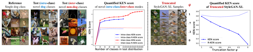
Figure 7: Quantified KEN score in real and generated distributions. Left: KEN score in ImageNet-1K. Intra-class means similarity in taxonomy (e.g. Dogs with different breeds). Right: KEN score in truncated StyleGAN-XL. $\psi$ is truncation factor. $\psi=1$ reduces to normal StyleGAN-XL. ”R-KEN” means switching test and reference distributions.

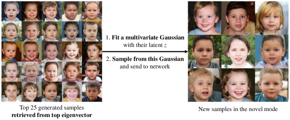
Figure 8: Generating new samples in a specific novel mode by fitting a Gaussian with samples from qualitative analysis.

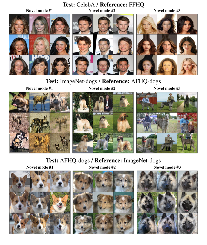
Figure 9: Novel modes between real datasets visualized with top-3-ranked eigenvectors. Extra samples of Figure 4.

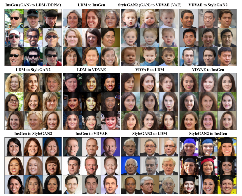
Figure 10: Novel modes between FFHQ-trained generative models in various architecture with the top-ranked eigenvector. Extra samples of Figure 5.

Table 2: Benchmarking fitness of generative models. Test distributions are generative models and reference distributions are their training sets. More powerful models tend to have lower KEN to the training set.

Dataset	Model	IS	FID	Precision	Recall	Density	Coverage	KEN
	GGAN [32]	6.51	40.22	0.56	0.30	0.42	0.31	3.03
	DCGAN [33]	5.76	51.98	0.62	0.16	0.56	0.25	3.02
	WGAN-WC [34]	3.99	95.69	0.53	0.04	0.40	0.11	3.01
	WGAN-GP [23]	7.04	26.42	0.62	0.56	0.55	0.46	2.99
	ACGAN [35]	7.02	35.42	0.60	0.23	0.50	0.32	2.99
	LSGAN [36]	7.13	31.31	0.61	0.41	0.50	0.42	2.97
	LOGAN [37]	7.95	17.86	0.64	0.64	0.60	0.56	2.90
	SAGAN [38]	8.67	9.58	0.69	0.63	0.72	0.72	2.70
	SNGAN [39]	8.77	8.50	0.71	0.62	0.79	0.75	2.65
	BigGAN [31]	9.14	6.80	0.71	0.61	0.86	0.80	2.59
	ContraGAN [40]	9.40	6.55	0.73	0.61	0.87	0.81	2.57
CIFAR10	StyleGAN2-ADA [41]	10.14	3.61	0.73	0.67	0.98	0.89	2.50
	SAGAN [38]	14.47	64.04	0.33	0.54	0.16	0.14	3.46
	StyleGAN2-SPD [19]	21.08	35.27	0.50	0.62	0.37	0.33	3.17
	StyleGAN3-t-SPD [42]	20.90	33.69	0.52	0.61	0.38	0.32	3.13
	SNGAN [39]	32.28	28.66	0.54	0.67	0.42	0.41	3.07
	ContraGAN [40]	25.19	28.33	0.67	0.53	0.64	0.34	2.91
	ReACGAN [43]	52.95	18.19	0.76	0.40	0.88	0.49	2.67
	BigGAN-2048 [31]	104.57	11.92	0.74	0.40	0.98	0.75	2.56
ImageNet $128^{2}$	StyleGAN-XL [28]	225.16	2.71	0.80	0.63	1.12	0.93	2.42

References

- [1] Diederik P Kingma and Max Welling. Auto-encoding variational bayes. arXiv preprint arXiv:1312.6114, 2013.
- [2] Ian Goodfellow, Jean Pouget-Abadie, Mehdi Mirza, Bing Xu, David Warde-Farley, Sherjil Ozair, Aaron Courville, and Yoshua Bengio. Generative adversarial nets. Advances in neural information processing systems, 27, 2014.
- [3] Jonathan Ho, Ajay Jain, and Pieter Abbeel. Denoising diffusion probabilistic models. Advances in neural information processing systems, 33:6840–6851, 2020.
- [4] Martin Heusel, Hubert Ramsauer, Thomas Unterthiner, Bernhard Nessler, and Sepp Hochreiter. Gans trained by a two time-scale update rule converge to a local nash equilibrium. Advances in neural information processing systems, 30, 2017.
- [5] Mikołaj Bińkowski, Danica J Sutherland, Michael Arbel, and Arthur Gretton. Demystifying mmd gans. arXiv preprint arXiv:1801.01401, 2018.
- [6] Tim Salimans, Ian Goodfellow, Wojciech Zaremba, Vicki Cheung, Alec Radford, Xi Chen, and Xi Chen. Improved techniques for training GANs. In D. Lee, M. Sugiyama, U. Luxburg, I. Guyon, and R. Garnett, editors, Advances in Neural Information Processing Systems, volume 29. Curran Associates, Inc., 2016.
- [7] Mehdi SM Sajjadi, Olivier Bachem, Mario Lucic, Olivier Bousquet, and Sylvain Gelly. Assessing generative models via precision and recall. Advances in neural information processing systems, 31, 2018.
- [8] Tuomas Kynkäänniemi, Tero Karras, Samuli Laine, Jaakko Lehtinen, and Timo Aila. Improved precision and recall metric for assessing generative models. Advances in Neural Information Processing Systems, 32, 2019.
- [9] Muhammad Ferjad Naeem, Seong Joon Oh, Youngjung Uh, Yunjey Choi, and Jaejun Yoo. Reliable fidelity and diversity metrics for generative models. In International Conference on Machine Learning, pages 7176–7185. PMLR, 2020.
- [10] Ali Borji. Pros and cons of gan evaluation measures: New developments. Computer Vision and Image Understanding, 215:103329, 2022.
- [11] Mohammad Jalali, Cheuk Ting Li, and Farzan Farnia. An information-theoretic evaluation of generative models in learning multi-modal distributions. In Thirty-seventh Conference on Neural Information Processing Systems, 2023.
- [12] Ahmed Alaa, Boris Van Breugel, Evgeny S Saveliev, and Mihaela van der Schaar. How faithful is your synthetic data? sample-level metrics for evaluating and auditing generative models. In International Conference on Machine Learning, pages 290–306. PMLR, 2022.
- [13] Casey Meehan, Kamalika Chaudhuri, and Sanjoy Dasgupta. A non-parametric test to detect data-copying in generative models. In International Conference on Artificial Intelligence and Statistics, 2020.
- [14] Marco Jiralerspong, Joey Bose, Ian Gemp, Chongli Qin, Yoram Bachrach, and Gauthier Gidel. Feature likelihood score: Evaluating the generalization of generative models using samples. In Thirty-seventh Conference on Neural Information Processing Systems, 2023.
- [15] Jiyeon Han, Hwanil Choi, Yunjey Choi, Junho Kim, Jung-Woo Ha, and Jaesik Choi. Rarity score : A new metric to evaluate the uncommonness of synthesized images. In The Eleventh International Conference on Learning Representations, 2023.
- [16] Alex Krizhevsky, Geoffrey Hinton, et al. Learning multiple layers of features from tiny images. 2009.
- [17] Jia Deng, Wei Dong, Richard Socher, Li-Jia Li, Kai Li, and Li Fei-Fei. Imagenet: A large-scale hierarchical image database. In 2009 IEEE conference on computer vision and pattern recognition, pages 248–255. Ieee, 2009.
- [18] Ziwei Liu, Ping Luo, Xiaogang Wang, and Xiaoou Tang. Deep learning face attributes in the wild. In Proceedings of the IEEE international conference on computer vision, pages 3730–3738, 2015.
- [19] Tero Karras, Samuli Laine, and Timo Aila. A style-based generator architecture for generative adversarial networks. In Proceedings of the IEEE/CVF conference on computer vision and pattern recognition, pages 4401–4410, 2019.
- [20] Yunjey Choi, Youngjung Uh, Jaejun Yoo, and Jung-Woo Ha. Stargan v2: Diverse image synthesis for multiple domains. In Proceedings of the IEEE/CVF conference on computer vision and pattern recognition, pages 8188–8197, 2020.
- [21] Christian Szegedy, Vincent Vanhoucke, Sergey Ioffe, Jon Shlens, and Zbigniew Wojna. Rethinking the inception architecture for computer vision. In Proceedings of the IEEE conference on computer vision and pattern recognition, pages 2818–2826, 2016.
- [22] MinGuk Kang, Joonghyuk Shin, and Jaesik Park. StudioGAN: A Taxonomy and Benchmark of GANs for Image Synthesis. IEEE Transactions on Pattern Analysis and Machine Intelligence (TPAMI), 2023.
- [23] Ishaan Gulrajani, Faruk Ahmed, Martin Arjovsky, Vincent Dumoulin, and Aaron C Courville. Improved training of wasserstein gans. Advances in neural information processing systems, 30, 2017.
- [24] Tuomas Kynkäänniemi, Tero Karras, Samuli Laine, Jaakko Lehtinen, and Timo Aila. Improved Precision and Recall Metric for Assessing Generative Models. Curran Associates Inc., Red Hook, NY, USA, 2019.
- [25] Ceyuan Yang, Yujun Shen, Yinghao Xu, and Bolei Zhou. Data-efficient instance generation from instance discrimination. arXiv preprint arXiv:2106.04566, 2021.
- [26] Robin Rombach, Andreas Blattmann, Dominik Lorenz, Patrick Esser, and Björn Ommer. High-resolution image synthesis with latent diffusion models, 2021.
- [27] Rewon Child. Very deep vaes generalize autoregressive models and can outperform them on images. arXiv preprint arXiv:2011.10650, 2020.
- [28] Axel Sauer, Katja Schwarz, and Andreas Geiger. Stylegan-xl: Scaling stylegan to large diverse datasets. In ACM SIGGRAPH 2022 conference proceedings, pages 1–10, 2022.
- [29] Alan J Hoffman and Helmut W Wielandt. The variation of the spectrum of a normal matrix. In Selected Papers Of Alan J Hoffman: With Commentary, pages 118–120. World Scientific, 2003.
- [30] Marco Marchesi. Megapixel size image creation using generative adversarial networks. arXiv preprint arXiv:1706.00082, 2017.
- [31] Andrew Brock, Jeff Donahue, and Karen Simonyan. Large scale gan training for high fidelity natural image synthesis. arXiv preprint arXiv:1809.11096, 2018.
- [32] Jae Hyun Lim and Jong Chul Ye. Geometric gan. arXiv preprint arXiv:1705.02894, 2017.
- [33] Alec Radford, Luke Metz, and Soumith Chintala. Unsupervised representation learning with deep convolutional generative adversarial networks. arXiv preprint arXiv:1511.06434, 2015.
- [34] Martin Arjovsky, Soumith Chintala, and Léon Bottou. Wasserstein gan, 2017.
- [35] Augustus Odena, Christopher Olah, and Jonathon Shlens. Conditional image synthesis with auxiliary classifier gans. In International conference on machine learning, pages 2642–2651. PMLR, 2017.
- [36] Xudong Mao, Qing Li, Haoran Xie, Raymond YK Lau, Zhen Wang, and Stephen Paul Smolley. Least squares generative adversarial networks. In Proceedings of the IEEE international conference on computer vision, pages 2794–2802, 2017.
- [37] Yan Wu, Jeff Donahue, David Balduzzi, Karen Simonyan, and Timothy Lillicrap. Logan: Latent optimisation for generative adversarial networks. arXiv preprint arXiv:1912.00953, 2019.
- [38] Han Zhang, Ian Goodfellow, Dimitris Metaxas, and Augustus Odena. Self-attention generative adversarial networks. In International conference on machine learning, pages 7354–7363. PMLR, 2019.
- [39] Takeru Miyato, Toshiki Kataoka, Masanori Koyama, and Yuichi Yoshida. Spectral normalization for generative adversarial networks, 2018.
- [40] Minguk Kang and Jaesik Park. Contragan: Contrastive learning for conditional image generation, 2021.
- [41] Tero Karras, Miika Aittala, Janne Hellsten, Samuli Laine, Jaakko Lehtinen, and Timo Aila. Training generative adversarial networks with limited data, 2020.
- [42] Tero Karras, Miika Aittala, Samuli Laine, Erik Härkönen, Janne Hellsten, Jaakko Lehtinen, and Timo Aila. Alias-free generative adversarial networks. In Proc. NeurIPS, 2021.
- [43] Minguk Kang, Woohyeon Shim, Minsu Cho, and Jaesik Park. Rebooting acgan: Auxiliary classifier gans with stable training, 2021.