Geometry on surfaces, a source for mathematical developments
Abstract
We present a variety of geometrical and combinatorial tools that are used in the study of geometric structures on surfaces: volume, contact, symplectic, complex and almost complex structures. We start with a series of local rigidity results for such structures. Higher-dimensional analogues are also discussed. Some constructions with Riemann surfaces lead, by analogy, to notions that hold for arbitrary fields, and not only the field of complex numbers. The Riemann sphere is also defined using surjective homomorphisms of real algebras from the ring of real univariate polynomials to (arbitrary) fields, in which the field with one element is interpreted as the point at infinity of the Gaussian plane of complex numbers. Several models of the hyperbolic plane and hyperbolic 3-space appear, defined in terms of complex structures on surfaces, and in particular also a rather elementary construction of the hyperbolic plane using real monic univariate polynomials of degree two without real roots. Several notions and problems connected with conformal structures in dimension 2 are discussed, including dessins d’enfants, the combinatorial characterization of polynomials and rational maps of the sphere, the type problem, uniformization, quasiconformal mappings, Thurston’s characterization of Speiser graphs, stratifications of spaces of monic polynomials, and others. Classical methods and new techniques complement each other.
The final version of this paper will appear as a chapter in the Volume Surveys in Geometry. II (ed. A. Papadopoulos), Springer Nature Switzerland, 2024.
Keywords: geometric structure, conformal structure, almost complex structure (-field), Riemann sphere, uniformization, the type problem, rigidity, model for hyperbolic space, cross ratio, Belyi’s theorem, Riemann–Hurwitz formula, Chasles 3-point function, branched covering, type problem, dessin d’enfants, slalom polynomial, slalom curve, space of monic polynomials, stratification, fibered link, divide, Speiser curve, Speiser graph, line complex, quasiconformal map, almost analytic function.
AMS classification: 12D10, 26C10, 14H55, 30F10, 30F20, 30F30, 53A35, 53D30, 57K10,
1 Introduction
Given a differentiable surface, i.e., a 2-dimensional differentiable manifold, one can enrich it with various kinds of geometric structures. Our first aim in the present survey is to give an introduction to the study of surfaces equipped with locally rigid and homogeneous geometric structures.
Formally, a geometric structure on a surface is given by a section of some bundle associated with its tangent bundle . We shall deal with specific examples, mostly, volume forms, almost complex structures (equivalently, conformal structures, since we are dealing with surfaces) and Riemannian metrics of constant Gaussian curvature. We shall also consider quasiconformal structures on surfaces. Foliations with singularities, Morse functions, meromorphic functions and differentials on almost complex surfaces induce geometric structures that are locally rigid and homogeneous only in the complement of a discrete set of points on the surface. Laminations, measured foliations and quadratic differentials are examples of less homogeneous geometric structures. They play important roles in the theory of surfaces, as explained by Thurston, but we shall not consider them here.
A theorem of Riemann gives a complete classification of non-empty simply connected open subsets of that are equipped with almost complex structures. Only two classes remain! This takes care at the same time of the topological classification of such surfaces without extra geometric structure: they are all homeomorphic. The classical proof of this topological fact invokes the Riemann Mapping Theorem, that is, it assumes the existence of an almost complex structure on the surface. Likewise, only two classes remain in the classification of non-empty open connected and simply connected subsets of that are equipped with a Riemannian metric of constant curvature: the Euclidean and the Bolyai–Lobachevsky plane. The latter is also called the non-Euclidean or hyperbolic plane.
No classification theorem similar to that of simply connected open subsets of holds in , even if one restricts to contractible subsets. See [110] for the historical example, now called “Whitehead manifold”, which, by a result of Dave Gabai (2011) [37], is a manifold of small category, i.e., it is covered by two charts, both of which being copies of that moreover intersect along a third copy of .
We shall be particularly concerned with almost complex structures, i.e., conformal structures, on surfaces. The theory of such structures is intertwined with topology. This is not surprising: Riemann’s first works on functions of one complex variable gave rise at the same time to fundamental notions of topology. He conceived the notion of “-extended multiplicity” (Mannigfaltigkeit), an early version of -manifold, he introduced basic notions like connectedness and degree of connectivity for surfaces, which led him to the discovery of Betti numbers in the general setting (see Andé Weil’s article [109] on the history of the topic), he classified closed surfaces according to their genus, he introduced branched coverings, and he was the first to notice the topological properties of functions of one complex variable (one may think of the construction of a Riemann surface associated with a multi-valued meromorphic function). At about the same time, Cauchy, in his work on the theory of functions of one complex variable, introduced path integrals and the notion of homotopy of paths. We shall see below many such instances of topology meeting complex geometry.
In several passages of the present survey, we shall encounter graphs that are used in the study of Riemann surfaces. They will appear in the form of:
At several places, we shall see how familiar constructions using the field of complex numbers can be generalized to other fields. Conversely, algebraic considerations will lead to several models of the Riemann sphere and of 2- and 3-dimensional hyperbolic spaces. Relations with the theory of knots and links will also appear.
Let us give now a more detailed outline of the next sections:
In §2 we present a few classical examples of rigidity and local rigidity results in the setting of geometric structures on -dimensional manifolds. A theorem due to Jürgen Moser, whose proof is sometimes called “Moser’s Trick”, deals with the classification up to isotopy of volume forms on compact connected oriented -dimensional manifolds. We show how this proof can be adapted to the symplectic and contact settings. A local rigidity result (which we call a Darboux local rigidity theorem) gives a canonical form for volume, symplectic and contact forms on non-empty connected and simply connected open subsets of .
In dimension two, almost complex structures are also locally rigid, and we present a Darboux-like theorem for them. The question of the existence and integrability of -structures on higher-dimensional spheres arises naturally. We survey a result due to Adrian Kirchhoff which says that an -dimensional sphere admits a -structure if and only if the -dimensional sphere admits a parallelism, that is, a global field of frames. This deals with the question of the existence of -fields on higher-dimensional spheres, which we also discuss in the same section: only carries such a structure.
Section 3 is concerned with the first example of Riemann surface, namely, the Riemann sphere. We give several models of this surface. Its realization as the projective space leads to constructions that are valid for any field and not only for . In the same section, we review a realization of with its round metric as a quotient space of the group of linear transformations of of determinant 1 preserving the standard Hermitian product. The intermediate quotient is isometric to and also to the space of length tangent vectors to . In this description, oriented Möbius circles on (that is, the circles of the conformal geometry of ) lift naturally to oriented great circles on . Also, closed immersed curves without self-tangencies lift to classical links (that is, links in the 3-sphere).
In §4, we present another model of the Riemann sphere, together with models of the hyperbolic plane and of hyperbolic 3-space. A model of the Riemann sphere is obtained using algebra, namely, fields and ring homomorphisms. In this model, the point at infinity of the complex plane is represented by , the field with one element. The notion of shadow number is introduced, as a geometrical way of viewing the cross ratio. The hyperbolic plane appears as a space of ideals equipped with a geometry naturally given by a family of lines. In this way, the hyperbolic plane has a very simple description which arises from algebra. The cross ratio is used to prove a necessary and sufficient condition for a generic configuration of planes in a real 4-dimensional vector space to be a configuration of complex planes. We then introduce the notions of compatible (or -conformal) Riemannian metric and we prove the existence and uniqueness of such metrics on homogeneous Riemann surfaces with commutative stabilizers. We describe several models of spherical geometry (surfaces of constant curvature +1), and of 2- and 3-dimensional hyperbolic spaces in terms of the complex geometry of surfaces. We then study the notion of -compatible Riemannian metrics. An existence result of such metrics is the occasion to characterize homogeneous Riemann surfaces up to bi-holomorphic equivalence.
In §5, we reduce generality by assuming that the surface is an open connected and path-connected non-empty subset of the real plane . Fundamental results appear. For instance, the theorem saying that two open connected and path-connected non-empty subsets of the real plane are diffeomorphic, a consequence of the Riemann Mapping Theorem. This theorem says that any nonempty open subset of the complex plane which is not the entire plane is biholomorphically equivalent to the unit disc. The Riemann Mapping Theorem generalized to any simply connected Riemann surface (and not restricted to open subsets of the plane) is the famous Uniformization Theorem. It leads to the type problem, which we consider in §7.
The next section, §6, is concerned with some aspects of branched coverings between surfaces. A classical combinatorial formula associated with such an object is the Riemann–Hurwitz formula. It leads to some natural problems which are still unsolved. A combinatorial object associated with a branched covering of the sphere is a Jordan curve that passes through all the critical values and which we call a Speiser curve. Its lift by the covering map is a graph we call a Speiser graph, an object that will be used several times in the rest of the survey. A theorem of Thurston which we recall in this section gives a characterization of oriented graphs on the sphere that are Speiser graphs of some branched covering of the sphere by itself. Thurston proved this theorem as part of his project of understanding what he called the “shapes” of rational functions of the Riemann sphere. In the same section, we introduce a graph on a surface which is dual to the Speiser graph, often known in the classical literature under the name line complex, which we use in an essential way in §7. We reserve the name line complex to another graph.
The type problem, reviewed in §7, is the problem of finding a method for deciding whether a simply connected Riemann surface, defined in some specific manner (e.g., as a branched covering of the Riemann sphere, or as a surface equipped with some Riemannian metric, or obtained by gluing polygons, etc.) is conformally equivalent to the Riemann sphere, or to the complex plane, or to the open unit disc. We review several methods of dealing with this problem, mentioning works of Ahlfors, Nevanlinna, Teichmüller, Lavrentieff and Milnor. Besides the combinatorial tools introduced in the previous sections (namely, Speiser graphs and line complexes), the works on the type problem that we review use the notions of almost analytic function and quasiconformal mapping.
In the last section, §8, combinatorial tools are used for other approaches to Riemann surfaces, in particular, in the theory of dessins d’enfants, in applications to knots and links and in the theory of slalom polynomials. Two different stratifications of the space of monic polynomials are presented.
2 Rigidity of geometric structures
In this section, we give several examples of locally rigid structures on surfaces. A classical example of a non-locally rigid structure is a Riemannian metric on any manifold of dimension .
2.1 Volume, symplectic and contact forms
Moser’s theorem says that only the total volume of a smooth volume form on a connected compact manifold matters, namely, two volume forms of equal total volume are isotopic. More precisely:
Theorem 2.1 (J. Moser [75])
Let be a compact connected oriented manifold of dimension equipped with two smooth volume forms and of equal total volume. Then there exists an isotopy satisfying . In particular, we have .
-
Proof
Clearly for some positive function , since for any and for any oriented frame at we have and . It follows that is a path of volume forms that connects the form to the form and we have
Thus, the de Rham cohomology class vanishes on the connected manifold , therefore there exists a smooth -form with . Hence, .
In order to construct the required isotopy satisfying , we need a time-dependent vector field whose flow induces the isotopy and such that the equality holds. Differentiating, using the Cartan formula and the fact that , yields
The family of vector fields defined by satisfies the above equation. The equation has, for a given -form , has a unique solution, since for each , is a non-degenerate volume form. Therefore the family of forms is constant, hence as required.
The above result also holds for a symplectic form, that is, a closed nondegenerate differential 2-form, at the price of a stronger assumption. The proof works verbatim. Thus we get:
Theorem 2.2 (J. Moser)
Let be a compact connected oriented manifold of dimension equipped with two symplectic forms and of equal periods, i.e., with equal de Rham cohomology classes. Assume that the forms are connected by a smooth path of symplectic forms with constant periods, i.e., for all , in . Then there exists an isotopy with . In particular, .
The so-called “Moser trick” works as a “simplification by d” in the equation and it amounts to noticing that for a volume form and for an -form the equation has a unique solution .
From symplectic structures, we pass to contact forms and contact structures.
A contact form on an -dimensional manifold is a pointwise non-vanishing differential -form such that at each point in the restriction of to the kernel of is non-degenerate.
A contact structure on is a distribution of hyperplanes in the tangent bundle given locally as a field of kernels of a contact form.
Moser’s method also works, even more simply, without “trick” and without extra stronger assumption, for families of contact structures and it gives another proof of the Gray stability theorem for contact forms [39]:
Theorem 2.3 (J. W. Gray [39])
Let be a smooth family of contact forms on a compact manifold . Then there exists a -dependent vector field on with flow and . In particular, there exists a family of positive functions such that for all , .
-
Proof
A measure for the variation of the kernel of is the restriction of to the kernel . By the non-degeneration of the restriction , there exists a unique -dependent vector field in the distribution (that is, the family of subspaces) with . Hence the kernels of do not vary since .
For more applications, see [71]. The use of a proper exhaustion allows us to extend the above theorem to pairs of volume forms on connected non-compact manifolds of equal finite or infinite total volume.
Furthermore, the above proofs work also in a relative version: if the forms coincide on a closed subset , then the time-dependent vector field vanishes along the subset and generates a flow that fixes the subset . The Darboux type rigidity theorems for volume, symplectic and contact forms follow:
Theorem 2.4 (Local Darboux rigidities)
Let be a volume or a symplectic form, and let be a contact form on an -, - or -manifold respectively. Then at each point of there exists a coordinate chart or or respectively such that the volume form is expressed by , the symplectic form by and the contact form by .
- Remark
The classical Darboux theorem holds in the setting of symplectic geometry, see [29]. This theorem says that any symplectic manifold of dimension is locally isomorphic (in this setting, it is said to be symplectomorphic) to the linear symplectic space equipped with its canonical symplectic form . As a consequence, any two symplectic manifolds of the same dimension are locally symplectomorphic to each other.
2.2 Almost complex structures
An almost complex structure on a differentiable surface is an endomorphism of the tangent bundle of satisfying . More precisely, is a smooth family of endomorphisms of tangent spaces such that at each point , we have . The standard example is where is the constant family of endomorphisms given by the matrix . This corresponds to the plane equipped with multiplication by .
The following proof is not based upon the above method.
Theorem 2.5
Local -rigidity in real dimension 2. Let be an almost complex structure on a surface . Then at each point there exists a coordinate chart such that holds.
-
Proof
(Sketch) First construct, using a partition of unity, an almost complex structure on the torus such that the structures and are isomorphic when restricted to open neighborhoods of on and of on . Let be a volume form on and let be the associated Riemannian metric . Let be the real function on satisfying and solving the partial differential equation
where is the Gaussian curvature of the metric . By the Gauss–Bonnet Theorem, , therefore the equation admits a solution by Fourier theory. Now use the Gauss curvature formula:
The metric has constant curvature , therefore is bi-holomorphic to for some lattice (a 2-generator discrete subgroup), which shows the statement for a local chart at , and hence also for a local chart at any .
For a detailed proof of Theorem 2.5, see [8, p. 114-117]. This theorem shows that every almost complex structure on a differentiable surface determines in a unique way a holomorphic structure in the usual sense (that is, a structure defined by an atlas of local charts with values in and holomorphic local changes).
Exercise 1: Give a proof of Theorem 2.5 using Moser’s trick.
Historical note The first definition of an almost complex structure is due to Charles Ehresmann who addressed the question of the existence of a complex analytic structure on a topological (resp. differentiable) manifold of even dimension, from the point of view of the theory of fiber spaces; cf. Ehresmann’s talk at the 1950 ICM [33]. Ehresmann mentions the fact that H. Hopf addressed the same question from a different point of view. He notes in the same paper that by a method proper to even-dimensional spheres he showed that the 4-dimensional sphere does not admit any almost complex structure, a result which was also obtained by Hopf using different methods. See also McLane’s review of Ehresmann’s work [82]. Ehresmann and MacLane also refer to the work of Wen-Tsün Wu [111, 112], who was a student of Ehresmann in Strasbourg.
2.3 Almost complex structures on -spheres
The existence and integrability of -structures in dimension 2 is very special. We mentioned that the -sphere does not admit any -field (Ehresmann and Hopf), but the -sphere does.
Clearly only spheres of even dimension can carry -fields. Adrian Kirchhoff, in his PhD thesis (ETH Zürich 1947) [55] established a relationship between two non-obviously related structures on spheres and of different dimensions; we report on this now.
Recall that a parallelism on a smooth -manifold is a global field of frames, that is, a field of tangent vectors which form a basis of the tangent space at each point.
Theorem 2.6 (Kirchhoff [56])
The sphere admits a -field if and only if the sphere admits a parallelism.
-
Proof
The case is special: the tangent space is of dimension , therefore is a -field and admits a parallelism.
“Only if” part for : In with the standard basis , let be the unit sphere in the span . Let be the unit sphere of . Assume that is a -field on . Let be the continuous map satisfying defined as follows:
-
–
First, for , seen as the equator of , we set
,
. -
–
For , we can write We then set
.
We have for , hence for , since the eigenvalues are . Observe that and . The differential at of maps the space onto an affine space of dimension in that intersects transversely the ray . Then, for , the images define a frame in by the projection parallel to onto .
“If” part: Work backwards.
-
–
In fact, by a celebrated result of Jeffrey Frank Adams [1], only the spheres admit a parallelism. This implies that does not admit any -field and does. Adams’ result was obtained several years after Kirchhoff’s result.
The question of the existence of a complex structure on is still wide open. How the Nijenhuis integrability condition for a -field on translates into a property of framings on is the subject of a recent paper [65].
We end this section on rigidity by a word on exotic spheres: Any two differentiable manifolds of the same dimension are locally diffeomorphic. But such manifolds may be homeomorphic without being diffeomorphic. The first examples of such a phenomenon are Milnor’s exotic 7-spheres [73]. In later papers, Milnor constructed additional examples.
3 The first compact Riemann surface
A Riemann surface is a complex 1-dimensional real manifold, or a 2-dimensional manifold equipped with a complex 1-dimensional structure, that is, an atlas whose charts take values in the Gaussian plane , with holomorphic transition functions.
In this section, we shall deal with the simplest Riemann surface, the Riemann sphere.
3.1 The Riemann sphere
The familiar round sphere in 3-space, together with its group of rigid motions, can be seen as a holomorphic object: its motions are angle-preserving. It is also a one-point compactification of the field of complex numbers. We shall see that this construction as a one-point compactification can be generalized to an arbitrary field.
First we ask the question:
Why do we need the Riemann sphere?
The statement: “Every sequence of complex numbers has a convergent subsequence” is very true, indeed true for bounded sequences. The statement is salvaged without this assumption if we introduce a wish object with the property that every sequence of complex numbers, for which no subsequence converges to a complex number, converges to . In this way, from the familiar Gaussian plane , we gain a new space, in which the above statement improves from very true to true. This topological construction is the familiar one-point compactification of non compact but locally compact spaces.
Very true is also the statement: “The ratio is well defined as long as ”. Again the statement becomes true if we introduce by wish a new object with This algebraic construction applies to any field , and not only .
In both constructions the object appears as a newcomer, an immigrant, with a special restricted status.
It is Riemann who gave an interpretation of the new set together with a very rich structure on it, for which the new element gains unrestricted status. In short, the automorphism group of acts transitively on this space, that is, the space is homogeneous.
The above topological construction also shows that the newcomer is above any bound, so from now on we use the symbol for .
Here is another construction of an infinity, valid for any field.
Let be a field. An element can be interpreted as a linear map . Its graph is the vector subspace of dimension in . So we get an embedding of the field in the projective space of all -dimensional vector subspaces in . The vector subspace is the only one which is not in the image of the embedding .
The element can be retrieved from as a slope: indeed, for any , if then and .
So the missing vector subspace corresponds to the forbidden fraction and can be called .
In the case where , this is the well-known embedding of in the circle of directions up to sign. Extending by gives the interpretation of as the projective space . Each linear automorphism of the -vector space induces a self-bijection of . If the matrix of is the -matrix , then with . The transformation or is called a fractional linear or Möbius transformation. Note that in particular .
Given a general field , an important structure on is provided by a -point function which we shall study in §4.3.
At this stage, we restrict to the case . The above construction of for an arbitrary field gives the familiar construction of , where denotes the multiplicative group of nonzero complex numbers.
The set carries many structures. First, there is the structure of a differentiable manifold given by the following atlas: We set and . Observe that and that every is of the type for .
Define maps by and by . Both maps are bijections. For the two maps are related; indeed, . It follows that the system is an atlas for a manifold structure with coordinates functions . Its quality is hidden in the quality of the coordinate change. For , from the above implicit relation it follows that . This coordinate change is differentiable; therefore is a smooth manifold with charts in the Gaussian plane .
The smooth -dimensional real manifold is diffeomorphic to the unit sphere in the three-dimensional real vector space . More precisely, the coordinate change is given in terms of the natural coordinate on , by . The smooth map is moreover holomorphic, so the above atlas provides with the structure of a Riemann surface. This Riemann Surface is the Riemann Sphere.
Let be an open subset of the Gaussian plane . Riemann defined a map to be holomorphic without using an expression that evaluates the map at given points. The idea is the following. The real tangent bundles and come with a field of endomorphisms. (The notation stands for “multiplication by ”.) The value of the field at the point is the linear map . To be holomorphic by Riemann’s definition is given by the following property of the differential:
In words, this means that the differential is -linear.
Riemann’s characterization of holomorphic maps together with the local -Rigidity Theorem 2.5 allows us to define a Riemann surface as a real 2-dimensional differentiable manifold equipped with a smooth field of endomorphisms of its tangent bundle satisfying .
The Riemann Sphere is the first example of a compact Riemann surface. The most familiar non-compact Riemann surface is the Gaussian plane . Another most important Riemann surface is the unit disc in . This is also the image of the southern hemisphere by the stereographic projection from the North pole onto a plane passing through the equator. This projection is holomorphic. The importance of the unit disc stems from the fact that it is equipped with the Poincaré metric, which makes it a model for the hyperbolic plane.
3.2 The group and its action on the Riemann sphere.
Now that we are familiar with the Riemann sphere, we study a group action on it.
Let be the usual Hermitian product on . This is the complex bilinear form on defined by . The Hermitian perpendicular to a complex vector subspace is again a complex vector subspace.
The group of determinant linear transformations of that preserve is the group consisting of all matrices of the form . This group acts on the Riemann sphere by Möbius transformations, in fact, by rotations. The map defines a diffeomorphism and induces a Lie group structure on the sphere .
The group acts transitively by conformal automorphisms on the Riemann sphere . The stabilizer of in is the group , which is isomorphic to the group of complex numbers of norm . The quotient construction induces a Riemannian metric on
A marked element in is a pair where and . Note that this representation is redundant since determines .
The group acts simply transitively on marked elements in .
The involution extends to marked elements: map first to and next to with .
A marked element determines a path in by , which in fact is a simple closed curve. Its velocity at is a length tangent vector . Observe that and . The path lifts to , which is a geodesic from to perpendicular to the foliation on by the Hopf circles . Hopf circles map to points, and geodesics map to simple closed geodesics in .
The map induces a bijection onto the length vectors to . Observe that acts almost simply transitively on length tangent vectors to . The quotient group acts simply transitively on length tangent vectors.
4 All three planar geometries and hyperbolic 3-space simultaneously
4.1 A stratification of the Riemann sphere arising from algebra
Bernhard Riemann was aware of the (Riemann) sphere being the complex plane union a point at infinity. His point of view on complex analysis was very geometric. In this section, we wish to describe an incarnation of the Riemann sphere which arises from algebra. For more details on this model, see [8, Chap. 3, §3.1] and [9, Chap. 1, §8.3].
The starting object is the set of surjective ring homomorphisms from the ring of polynomials in one unknown with real coefficients to a field . On the set we introduce two equivalence relations. The first relation, , declares and to be equivalent if there exists a field isomorphism with .
The relation holds if and only if the ideals in are equal.
The second relation, , requires and moreover holds in .
Up to field isomorphism, there are only three fields, , that are hit by a surjective ring homomorphism , namely, the fields , and where is the field with one element, that is, the field where holds. The field corresponds to the ideal consisting of the whole ring, which is prime, maximal but not proper.
-
Exercise
The two fields have only the identity as automorphism and the field only two automorphisms as -algebra, but as many field automorphisms as the power set of the real numbers.
In the following we will describe the quotient sets together with natural structures on these sets.
All ideals in are principal, that is, any such ideal is generated by a single element (it is obtained by multiplication of such an element by an arbitrary element of the ring). Kernels of are prime ideals, that is, the quotient of by such an ideal is an integral domain (the product of any two nonzero elements is nonzero). Thus, we have three kinds of kernels of , namely, , , and . Therefore the set is identified with . Here we use the notation for the upper/lower half planes.
The kernel of the ring homomorphism is not sufficient in order to describe its class in if . One needs moreover to specify a root or . Thus the set is a disjoint union of strata .
The fields are realized as sub--algebras in , so an alternative description of the set is the set of -algebra homomorphism from to .
We shall see that the set and its strata carry a rich panoply of structures. The set is identified with the Riemann sphere . Structures, such as the Chasles three point function (defined below) on , or the hyperbolic geometry on , will appear naturally. Naturally means here that the construction that leads to the structure commutes with the -algebra automorphisms of . For instance, it commutes with the substitutions that consist in translating to or with stretching to . The ideal maps to the ideal by translation and to by stretching.
A first example is the Chasles -point function on the stratum consisting of the ideals defined as follows: Given three distinct such points, , define .
In words, is the ratio of the monic generators of and evaluated at the zero of the monic generator of .
The next example is the -point function cross ratio : for distinct points , define . In words, this is Chasles evaluated at the first three points times Chasles evaluated at the last three points in the reverse order. It is truly a remarkable fact that the cross ratio function extends to a -point real function on and to a -point complex function on if one transfers the above wishful calculus with to .
The multiplicative monoid of polynomials which do not vanish at has also automorphisms that do not directly fit with the interpretation as polynomials with unknown . In particular, they are not ring automorphisms, but monoid automorphisms. A main example is the twisted palindromic symmetry: perform on a polynomial the substitution , followed by stretching with factor . (The palindromic symmetry is said to be twisted, because of the minus signs.) Then the ideal maps to the ideal . The Chasles function restricted to does not commute with the symmetry , but the cross ratio commutes. (This property is among the ones that make the cross ratio more natural than the Chasles -point function.) This symmetry, which is an involution, extends to a fixed point free involution of . Remarkably, the symmetry commutes with the cross ratio . In this sense, is more natural than .
The above operations of real translation and stretching, i.e., substituting for or for with , together with the twisted palindromic symmetry induce bijections of the set of monic polynomials of degree without real roots. Composing these bijections generates a group . It is a remarkable fact that this group is, as an abstract group, isomorphic to the group . It is also a remarkable fact that the abstract group carries a unique structure of Lie group. So there is also a topology on , which allows us to define the subgroup as the connected component of the neutral element in the Lie group . The group is isomorphic to the group .
The fixed point free involution on extends to by putting for an involution with as unique fixed point.
The group acts transitively and faithfully on the above strata and on . From this action one gets a topology on the strata and also, as we will explain, a geometry on . It is also remarkable that this geometry, in fact, the planar hyperbolic geometry, can also be explained in a more elementary way in term of the interpretation as ideals.
The action of on is the so-called modular action of on . Thinking of an element as a real matrix of determinant up to sign, , the action on is given by .
The modular action of on extends to the projective action of on and also to the projective action of the complex group on .
The hyperbolic geometry on can also be defined in terms of ideals in the following rather elementary way.
Points are the elements of . The monic generator of the corresponding ideal may be denote by .
The notion of line is introduced using convex combinations. More precisely, given two distinct points , the line through them is defined as follows:
Denote by the convex combination of the polynomials . Note first that any polynomial obtained in this way is monic. Let be the maximal interval on which has no real roots. Note that (one may start by checking that for and there are no real roots). This implies that the cross ratio is a positive real number . If define . If let be the zero of and define .
With such a definition, the axiom of hyperbolic geometry saying that for any two distinct points there is a unique line passing through them is trivially satisfied.
-
Exercise
For a better understanding of this construction of the hyperbolic plane, please check that the root of travels along for in case . Note that is a half circle in with centre in .
The hyperbolic Riemannian metric is the Hessian at of the function .
In this model, we can define the hyperbolic distance between and as . We can make a relation with the model of the hyperbolic plane that uses the Hilbert metric. In this way we have all the ingredients of hyperbolic geometry based on elementary algebra, that can be taught at high-school.
-
Remark
The above twisted palindromic map induces an involution on , the complement of the hypersurface of polynomials that vanish at . Therefore, is a birational involution and the above constructions would generate subgroups , etc. in the Cremona group of birational transformations of . Thus, the artefact of defining can be avoided. Even better, the geometry of Cremona groups is hyperbolic. For the Cremona group, see [21, 22, 26, 30, 94, 106, 113].
4.2 A note on the field with one element
The importance of the field with one element , which was interpreted in the above construction of the Riemann sphere as the point at infinity of the complex plane, was first highlighted by Jacques Tits in his paper [104]. In this paper, Tits proposed the development of a geometry over the field which would be the limit of geometries over the finite fields , where denotes the field of cardinality where is a positive prime. Note that if we make tend to in the notation , , we obtain , which is an indication of the fact that the field may be considered as a deformation of the field . One may also make an analogy with the fact that a limit is used in quantum topology for a geometric interpretation of the TQFT calculus of Turaev, Viro, Kauffman, etc. (The analogy is vague, but this is the nature of analogies.)
After Tits introduced his idea of studying a geometry over the field , many works were done on this theme. For instance, Manin, in his lectures on the zeta function [70], proposed the study of a “Tate motive over a one-element field”. In the paper [28] titled Fun with by Connes, Consani and Marcolli, the field becomes an actor in an approach to the Riemann hypothesis.
4.3 The Riemann sphere and shadow numbers
Let be a -dimensional vector space over a field . If has or more elements, then the space of lines through the origin in has at least elements. We wish to define in a geometric way the cross ratio of a figure consisting of distinct lines in . This is done in the form of two exercises.
Exercise 1: Do the following: Identify with the Cartesian product of and , and let be the linear map from to that has as graph, . Define as the stretch factor of the linear map . This is represented in Figure 1, in which we start with the point on , with its image by and the image of by .
Please check now that if the lines are defined using a basis and “numbers” such that , then the formula holds.
In this way, we recover the usual formula for the cross ratio.
In the above construction of the cross ratio, the use of a Cartesian product and graphs of maps suggest that parallel lines are essential. This is not the case. For instance, the construction also works inside a Euclidean triangle with vertices , as in the following exercise, which asks for a construction of the cross ratio which is a projective version of the construction in Exercice 4.3, which is affine (it uses the notion of parallels):
Exercise 2: Let be interior points of the side of a triangle , put . Let be the segments connecting the vertex with .
Define as follows: Connect by a segment with which insects in . The half-line intersects in . Define in the same way . Now is not linear, but with fixed point . Define the cross ratio to be the stretch factor of the differential at of the map . The construction is represented in Figure 2, where, like in Figure 1, is a point in , its image by and the image of by .
It is important to observe that , in planar Euclidean geometry, does not depend upon the position of the side . This property does not hold in spherical or hyperbolic geometry. In spherical geometry there is a preferred choice for the side , namely, such that the triangle becomes bi-orthogonal. This was already done by Menelaus of Alexandria!
This construction also works for a configuration in general position of linear subspaces of dimension in a real vector space of dimension . The invariant is now an element . One may use this to prove the following:
Theorem 4.1
The four Complex Lines Theorem. Let be a generic labelled configuration of planes in a real -dimensional vector space . There exists a linear complex structure with (which means that each is a complex line) for every if and only if
or if is a multiple of the identity , for some .
The proof is contained in p. 73 of LABEL:A2021
Theorem 4.1 should be seen in the setting of the following general question: Given a -dimensional real vector space and a quadruple of 2-dimensional planes in satisfying some properties, does there exist an almost complex structure making such that are complex lines?
The usual formula for the cross ratio with numbers is memo-technically speaking a headache. A more geometrically-rooted name would be more satisfying. We propose shadow number: the shadow issued from a light bulb of four concurrent lines lying in a plane on a plane shows the same number. The proof uses the above special property in Euclidean geometry and becomes simplified if one uses the above geometric definition. If the name should remember a person, then perhaps Leonardo da Vinci number, for Leonardo studied central projections and perspectivities about years ago [67], or Menelaus number, for Menelaus studied shadows in spherical geometry about years ago. See [83] for the use by Menelaus of the invariance of the cross ratio in spherical geometry. Menelaus used this result in the proof of Proposition 71 of the Spherics,111Menelaus was extremely concise in his Spherics, and the proofs of some of the propositions in this work are very difficult to follow. This is why several results of the Spherics [85] were later explained and commented on by Arab mathematicians of the Middle Ages, after the Greek mathematical schools were desintegrated. Regarding this particular proposition, see the two papers [83, 84] and later medieval commentators, in an effort to provide full proofs of some of this and other difficult propositions in Menelaus’ Spherics, highlighted this invariance as a new proposition, in order to explain a proof in the Spherics; see Proposition 3.2 in [83] and [85, p. 356-360].
The group of linear transformations of acts on the Riemann sphere (see §4.1), since this group acts on complex lines through the origin of . From the geometric definition of the shadow number, it follows that this number is -invariant:
The shadow number is a -point function defined on the complement of the general diagonal in the Riemann sphere :
where is the subset of quadruples of points in with . Using the above formula one checks that the function is holomorphic with meromorphic extension to .
Exercise 3: For a triple of distinct points, study the partial function . What are the level sets of ?
Exercise 4: Reconstruct the complex structure of from the shadow function .
Exercise 5: For a point function , define to be the group of bijections satisfying . Consider the cases or or . Show that and .
4.4 -compatible metrics
In this section, is a differentiable compact connected surface equipped with a complex structure . A Riemannian metric on is called conformal with if for every point the map is -orthogonal. Thus, two metrics conformal with differ pointwise by a positive factor: for some function . A -calibrated volume form on , i.e., a differential 2-form satisfying gives by a Riemannian metric conformal with whose associated volume form is precisely . All metrics conformal with are obtained in a unique way from such a construction by taking for the oriented volume form of the Riemannian metric .
In conclusion, given , the space of Riemannian metrics conformal with is parametrized by the cone of -calibrated volume forms. In this way, the uniqueness is not only up to multiplying by a constant factor.
We wish to strengthen the notion of being “conformal with ” for metrics and gain back uniqueness or controlled non-uniqueness up to multiplying by a constant factor. This will be achieved first for Riemann surfaces that are homogeneous, i.e., whose group acts transitively on , such that moreover the stabilizers of points are compact.
The group of a connected Riemannian manifold is the group of diffeomorphisms that multiply the metric by a constant factor. Such diffeomorphisms are called similarities.
Theorem 4.2
Let be a homogeneous Riemann surface with commutative stabilizers. Then there exists a Riemannian metric conformal with such that . The Riemannian metric is unique up to multiplication by a constant factor.
-
Sketch of proof
The list of homogeneous connected Riemann surfaces up to bi-holomorphic equivalence is short:
-
1.
The Riemann sphere ;
-
2.
;
-
3.
;
-
4.
the infinite family of elliptic curves ;
-
5.
.
In this list, only the Riemann sphere has non-compact and non-commutative stabilizers—the stabilizer of a point is the affine group of . Thus, we do not need to consider this surface.
The second surface in the list is bi-holomorphic to . The Euclidean metric is up to multiplication by a constant factor the only metric whose bi-holomorphic equivalences are similarities. Note that its group of isometries is a strict subgroup of the group of similarities. It is not commutative. So we also do not consider this surface.
The third surface in the list is the image of the covering map with deck transformations . These deck transformations are isometries of the Euclidean metric, therefore they define a metric on which is locally Euclidean. This metric is defined by . Note the triple equality .
A similar discussion holds for the family of elliptic curves. In this case, instead of the mapping , one considers a mapping where is the group of translations generated by the complex numbers and .
The group acts transitively on by . The stabilizer of is the compact group . The Killing form on the Lie algebra induces on a Riemannian metric which is conformal with (“multiplication by ”). Again a triple equality of groups holds.
The interpretation of as a ring homomorphism and as an ideal (see §3.1) gives an elementary insight for the above explanation by Lie group theory.
Given , define the curve by the following: put , then are the roots in of the polynomials . Let be the maximal open interval containing the interval such that for all the convex combinations of polynomials have no real roots. Define as the path of roots in of the polynomials .
If , then the curve is the real half-line perpendicular to the real axis through and . If , then the curve is the semi-circle through with center on the real axis, hence perpendicular to the real axis.
The quantity defines a metric on , which is -invariant. The curves are length minimizing, hence geodesics. More precisely, the expansion of at the point gives the leading second order term and defines a Riemannian metric. From this, we can recover the hyperbolic metric on , see [9, §8.3].
-
1.
In conclusion, from the formulae and , each of the volume form and the metric is determined from the other one and from the almost complex structure . The same formulae determine from and because the 2-forms and are non-degenerate.
In fact, more generally, the motto is that in the triple of structures on surfaces (volume form , Riemannian metric , almost complex structure ) on , two elements determine the third one. The result is that there are fruitful interactions between symplectic geometry, Riemannian geometry and complex geometry. This is expressed in a spectacular manner in Gromov’s 1985 paper in which he introduced pseudo-holomorphic curves [44]. This introduced also notions of “positivity” and of “compactness” in the three geometrical settings. One result is that the stabilizers of and in , if they are related by a as above, coincide and form a maximal compact subgroup.
4.5 Spherical geometry
The differential sphere is present as the Riemann sphere . Spherical geometry is still missing. The group acts transitively on . The stabilizer is the group . Again by Lie theory, each maximal compact subgroup of defines a spherical metric on that is conformal with .
A perhaps more elementary approach is the following: Let be the space of fixed-point free involutions that preserve the shadow function . For two distinct involutions , the composition has two fixed points . Let be the determinants of the differentials at . Define the distance by
The space is a model for hyperbolic -space. The infinitesimal version of the metric is a Riemannian metric on . For each , the half-rays from define a diffeomorphism from the infinitesimal sphere with center to . The map is conformal and carries the spherical metric of to a metric on which is conformal with . Think of as the unit sphere in . The group is a maximal compact subgroup in . Moreover the equality holds.
We think of the Riemann sphere as the space of -dimensional vector subspaces in (§3.1). A positive Hermitian form on is a real bilinear map satisfying for
-
•
,
-
•
,
-
•
for .
A positive Hermitian form on defines by a fixed-point free involution of the Riemann sphere that preserves the shadow function . Here, associated with the complex line is the complex line . Two positive Hermitian forms that differ by a positive factor give the same involution.
Moreover the stabilizer in is a maximal compact subgroup in . Similar forms have the same stabilizers and all maximal compact subgroups correspond to a unique form.
If two lines in are neither perpendicular nor equal, they give by a quadruple of complex lines. The expression defines a function on with values in . The preimage of is the diagonal, the set of pairs with , and the preimage of the set of pairs with . Its infinitesimal version along the diagonal, i.e., at the Hessian of at , defines a Riemannian metric on which is similar, even isometric, to the spherical geometry of Gaussian curvature in dimension 2.
4.6 Models for hyperbolic 3-space and metrics of constant positive curvature on the sphere
Even though the 3-dimensional hyperbolic space does not admit a complex structure, its automorphism group is that of a complex manifold and is itself a complex Lie group, since we have
We have the following four models of the hyperbolic 3-space that arise from the complex geometry of surfaces; the first two models are geometric (they are defined in terms of group actions) whereas the other two use algebra:
-
1.
The space of fixed-point free shadow-preserving involutions of .
-
2.
The space of Riemannian metrics on that are conformal with and similar to the spherical metric.
-
3.
The space of similarity classes of positive Hermitian forms on .
-
4.
The space of maximal compact subgroups in (which is the automorphism group of the oriented hyperbolic 3-space).
The first model already appeared in §4.5, where we constructed the spherical geometry of the Riemann sphere. This is the sphere we called there. To get another point of view on this model, consider first the well-known Poincaré model of the hyperbolic space as a unit ball sitting in -space, with boundary the Riemann sphere . For each point in , an involution of is defined by assigning to each point in the intersection with the sphere of the line passing through this point and . To see that we get a model of , use the Hilbert metric model of this space.
For the second model, we also consider the Poincaré unit ball model of the hyperbolic space, with boundary the Riemann sphere . For each point of , we take the diffeomorphism which sends the infinitesimal round sphere (or a sphere in the tangent space) at that point to the boundary at infinity of the space, using the geodesic rays that start at this point. This is a conformal mapping. (One may prove this by trigonometry.) The mapping sends the conformal metric of the infinitesimal sphere to a metric on the sphere sitting at the boundary of the hyperbolic space. This construction commutes with the isometries of . It gives a 3-dimensional space of metrics in the same conformal class on . Thus, the hyperbolic -space appears as a space of metrics of curvature on . In other words, appears as a space of special metrics, i.e., as a moduli space, namely, the space of Riemannian metrics of Gaussian curvature on that are moreover in the conformal class of . Alternatively, the hyperbolic -space appears as the space of volume forms on such that the Riemannian metric defined by is a metric of Gaussian curvature .
For the third model, recall that a positive Hermitian form on is a Riemannian metric on such that one can measure the angle between two lines in this space. This model was explained in §3.2 above.
The fourth model is equivalent to the 3rd because the group acts on the space in question with stabilizer the automorphism group of the oriented hyperbolic 3-space, that is, the group quotiented by its maximal compact subgroup.
An explicit way of interconnecting the above models for the hyperbolic three-space is as follows.
Think of as the unit sphere in with its induced spherical metric together with the corresponding conformal structure, the space , for the Euclidean norm .
The stereographic projection with pole maps by
the factor conformally to . This projection extends to an (oriented) diffeomorphism
and equips by pullback the Riemann sphere with a Riemannian metric of Gaussian curvature .
Given an ordered triple of distinct points in , the shadow function gives by
a mapping such that the composition extends to a conformal diffeomorphism .
By pullback we obtain a family of Riemannian metrics of curvature on . Two such metrics and are related by an oriented isometry if and only if the composition is an oriented isometry of .
Now remember that the group of holomorphic automorphisms of is isomorphic to and acts simply transitively on triples of distinct points. So each triple is obtained in a unique way as from a chosen triple by applying a well-defined element . The above condition that the metrics and are related by an oriented isometry translates into the fact that and so it proves that the hyperbolic 3-space is parametrized by the symmetric space .
From the above discussion, some basic ingredients of the geometry of can be seen, such as the following:
-
•
Ideal points are the points of .
-
•
Given in , the points on the line from to are the metrics where varies over .
-
•
For , represented respectively by metrics and volume forms on , these points lie on where the points are the extrema of .
4.7 Models for the hyperbolic plane
The hyperbolic plane , like the 3-dimensional hyperbolic space , has also several interpretations in terms of the complex geometry of surfaces. A standard interpretation of is that it is the space of marked elliptic curves. We propose three other incarnations of this plane:
1. The hyperbolic plane is the space of ideals with its geometry naturally given by a family of lines . Indeed, the plane comes with a natural complex coordinate , defined by
The coordinate is a bijection with
as inverse. Thus, is the interpretation of the number as an ideal. See the details in §4.4 above.
2. The hyperbolic plane is the space of almost complex structures on (that is, endomorphisms of satisfying ) equipped with coordinates , and a volume form , and where is calibrated by the inequality for all .
Another way of seeing this is the following. We start by defining a map: , so that a point in the space has a coordinate where is the fixed point of for its homographic action on .
More explicitly, the matrix of in the basis is of the form where and (use the fact that the trace is zero), and is obtained from the fact that the determinant of the matrix is equal to 1. Such a matrix acts on the upper half-plane with exactly one fixed point, and we assign to this fixed point. It is possible to write explicitly the coordinates of this fixed point in terms of and .
Consider the map
where and is a complex coordinate. This is again a bijection, with inverse
and there is an interpretation of the number as a linear complex structure.
The incarnation is very helpful for the construction of hyperbolic trigonometry. Only High-school/Freshman knowledge is required in this construction.
This incarnation is also very helpful for the study of the space of complex structures on a given surface. As a first example, the surface itself has a complex structure. A tangent vector at is an endomorphism of such that the equation
holds at first order in . Therefore the tangent space at of is the vector space of endomorphisms that anti-commute with . The map is a canonical complex structure on which induces a complex structure on the infinite-dimensional manifold . This space is canonically path-connected. Indeed two structures are connected by the path that for is a geodesic in the space of linear complex structures on the oriented real vector space . The fact that the space is contractible now follows, since these canonical paths depend continuously upon endpoints.
3. The bijective coordinates on transport the geometries to a common geometry on . The coordinate is -holomorphic. The model with its conformal structure and hyperbolic metric, equipped with its action by the modular group , is a very appreciated model of the hyperbolic plane.
5 Uniformisation
5.1 Riemann’s uniformisation of simply connected domains
Theorem 5.1 (The Riemann Mapping Theorem [88])
Let be a non-empty open connected and simply connected subset of the complex plane which is not the entire plane. Let be a point in and a nonzero vector at . Then, there is a unique holomorphic bijection from to the unit disc such that and is a complex number which is real and positive.
Note that the inverse of a holomorphic bijection is also holomorphic (think of a holomorphic function as an angle-preserving map). Therefore the map is biholomorphic.
-
Outline, after Riemann’s proof, see [50]
This proof works in the case where is an open subset of the plane bounded by a Jordan curve (a simple closed curve). We outline this proof.
We wish to find a biholomorphic mapping which sends to .
Suppose that such a mapping exists. Separating the real and imaginary parts, we set
Applying a translation, we may assume that , therefore, . Applying a rotation, we may also assume that the vector of coordinate at is sent by to a vector pointing towards the positive real numbers.
Such a map , it is exists, is unique, since any holomorphic automorphism of the disc which fixes the origin is a rotation, and a rotation that fixes a direction is the identity.
Since is a bijection between and the unit disc, the point is the unique solution of the equation . Furthermore, the differential (or the complex derivative) of at is nonzero, otherwise would be non-injective in the neighborhood of zero. Thus, the function is holomorphic on . Since it does not take the value , a branch of its complex logarithm can be defined. Hence, there exists a holomorphic function on such that
In polar coordinates we can write , which gives
Separating the real and imaginary parts of as , we get
which we can write as
Notice that the function is identically zero on , since points on this curve satisfy .
Furthermore, the function is the real part of the holomorphic function , therefore it is harmonic at every point of .
Now given a harmonic function defined on the simply connected subset of the plane, there exists a unique holomorphic function which has this function as a real part. (The usual way to find this function is to use Cauchy’s theory of path integrals.)
Reasoning backwards, the problem of mapping to the unit disc can be solved if we can find a function which is harmonic on and which takes the values on .
In this way, Riemann reduced the problem of finding a holomorphic mapping from to to a problem of finding a harmonic function on with a prescribed value on . To find such a function, he appealed to the so-called Dirichlet method, which consists of considering the functional defined on the space of differentiable functions on by:
A function which realizes this infimum is harmonic.
- Remarks
1.— Riemann also used the Dirichlet principle in his existence proof of meromorphic functions on general Riemann surfaces, obtaining them from their real parts (harmonic functions). It was realized later that the Riemann Mapping Theorem and the existence of meromorphic functions are equivalent.
2.— A modern proof of the Riemann Mapping Theorem goes as follows (see Thurston’s notes[103]): Given a simply connected open strict subset of the complex plane and a point in , consider the set of functions
equipped with the topology of uniform convergence on compact sets. The desired conformal mapping is the mapping in this family that maximizes the modulus of the derivative . The existence of such a mapping uses the fact that for any family of holomorphic functions which is uniformly bounded on compact sets, every sequence has a subsequence which converges uniformly on compact sets to a holomorphic function (this is Montel’s theorem).
We shall call a Riemann mapping a biholomorphic mapping that sends the unit disc to a simply-connected subset of the plane (which we sometimes call a domain). This is the inverse of the mapping that we just considered.
For a general domain , the Riemann mapping is not explicit. In some special cases, there are explicit formulae, e.g., when is the upper half-plane, or a band in the plane (a region bounded by two parallel lines), or an angular sector (a connected component of the union of two intersecting Euclidean lines in the plane), or a domain bounded by two arcs of circle, or a sector of a disc, or a rectangle in the Euclidean plane, or a regular convex polygon, or a regular star polygon, or the interior of an ellipse or a parabola, and a few other cases. These examples and others are studied in the book by G. Julia [50].
There are also results that concern the boundary behavior of the Riemann mapping. The first name associated with such a boundary theory is Carathéodory. He proved that if the boundary of the domain is a Jordan curve, then the Riemann mapping extends continuously to a homeomorphism from the unit circle to the boundary of the domain. He also proved that in the general case the Riemann mapping extends continuously to the unit circle if and only if the boundary of the domain is locally connected (but this extension is generally not a homeomorphism). There are also measure-theoretic results and questions. For instance, in the case where the domain is bounded by a rectifiable curve , an extension of the Riemann mapping exists and sends any subset of measure zero (resp. of positive measure) of to a subset of measure zero (resp. of positive measure) of the circle. This was proved by Luzin and Privaloff [68] and by F. and M. Riesz [86]. One can also mention here the following result of Fatou [36]: If a function defined on the unit disc is holomorphic and bounded, then, at almost every point on the unit circle , the value of at a sequence of points converging to that point on a path which is not tangential to the unit circle has a limit. For an exposition of related results, see Chapter II of Lavrentieff’s book [64]. These results are useful in the modern developments of complex dynamics, in particular in the study of the conformal representation of the complement of the Julia set of a polynomial.
5.2 Uniformization of multiply connected domains
It is natural to search for generalizations of the Riemann Mapping Theorem for multiply connected open subsets of the plane. The first natural question is whether there exist canonical domains onto which they can be mapped biholomorphically, in analogy with the fact that the disc and the plane are canonical domains for simply connected domains. It is known that two open subsets of the complex plane that have the same connectivity are not necessarily conformally equivalent. For instance, two circular annuli (that is, annuli bounded by two concentric circles) are conformally equivalent if and only if they have the same modulus, that is, if and only if the ratio of their outer radius to their inner radius is the same. Thus, there are no canonical domains for multiply connected open subsets of the plane. However, there are figures which may be considered as “standard” domains for such subsets, and we now discuss some of them.
One of the oldest works on this question was done by Koebe, who studied in his papers [59], [60] and others conformal mappings of multiply connected open subsets of the plane onto circular domains, that is, multiply connected domains whose boundary components are all circles (which may be reduced to points). He proved that every finitely connected domain in the plane is conformally equivalent to a circular domain. The question of whether there is an analogous result for open subsets of the plane with infinitely many boundary components is still open. This question is known under the name Kreisnormierungsproblem, or the Koebe uniformization conjecture. Koebe formulated it in his paper [61]. The reader interested in this question may refer to the paper [23] by Ph. Bowers in which the author surveys several developments of this conjecture, including related works on circle packings by Koebe, Thurston and others. See also LABEL:Br1992.
H. Grötzsch, in his paper [41], works with two classes of domains which were considered by Koebe:
-
1.
Annuli with circular slits. These are circular annuli from which a certain number () of circular arcs (which may be reduced to points) centered at the center of the annulus, have been deleted.
-
2.
Annuli with radial slits. These are circular annuli from which a certain number () of radial arcs (which may be reduced to points) have been removed. Here, a radial arc is a Euclidean segment in the annulus which, when extended, passes through the center of the annulus.
The unit disc slit along an interval of the form () was employed by Grötzsch in [41] as a standard domain and is known under the name Grötzsch domain. Teichmüller, in his paper [101], calls a Grötzsch extremal region the complement of the unit disc in the Riemann sphere cut along a segment of the real axis joining a point to the point .
Another “standard model” for doubly connected domains is the Riemann sphere slit along two intervals of the form and where and are positive numbers. Such a domain is called a Teichmüller extremal domain by Lehto and Virtanen [66, p. 52]. In his paper [101], Teichmüller uses these domains in the study of extremal properties of conformal annuli. In the same paper, he works with other “standard” domains, e.g., the circular annulus cut along the segment joining to , where and are points on the real axis satisfying [101, §2.4]; see the discussion in Ahlfors’ book [14, p. 76].
5.3 Uniformization of simply connected Riemann surfaces
It is natural to consider conformal representations of surfaces that are not subsets of the complex plane. A wide generalization of the Riemann Mapping Theorem is the following, proved independently by Poincaré and Koebe:
Theorem 5.2 (Uniformization theorem)
Every simply connected Riemann surface can be mapped biholomorphically either to
-
1.
the Riemann sphere (elliptic case);
-
2.
the complex plane (parabolic case);
-
3.
the unit disc (hyperbolic case).
In each of these cases, the conformal biholomorphism from the model space onto the open Riemann surface is usually called a uniformizing map. Such a map associated to a Riemann surface is well defined up to composition by a conformal homeomorphism of the source. This implies that the mapping is determined in the first case by the images of three distinct points, in the second case by the image of two distinct points, and in the third case by the image of one point and a direction at that point.
If the Riemann surface is a simply connected open subset of the complex plane which is not the entire plane, then it is necessarily of hyperbolic type (this is the Riemann Mapping Theorem). Uniformizing maps for such surfaces have been particularly studied.
For a proof of the uniformization theorem based on a historical point of view, see the collective book [92]. For another point of view on uniformization (“uniformization by energy”), see [8, Chapter 10].
There are several open questions on the behavior of the uniformizing maps of simply connected surfaces equipped with Riemannian metrics. Lavrentieff, in his paper [63], adresses the question of the Lipschitz behavior of a uniformizing map . More precisely, he asks for conditions on the surface so that for any pair of points , the ratios and are bounded or unbounded (the distance in the disc being the Euclidean distance). To the best of our knowledge, this problem is still not settled.
6 Branched coverings
6.1 The Riemann–Hurwitz formula
The notion of branched covering between surfaces was conceived by Riemann. It will be used at several places in the rest of this chapter. We shall review in particular a theorem of Thurston on branched coverings of the sphere in relation with the question of the topological characterization of rational maps (§6.3). Branched coverings also appear in the study of the type problem (§7.2) and in the theory of dessins d’enfants (§8.1).
A map between two topological oriented surfaces is said to be a branched covering if it satisfies the following:
-
1.
for some discrete subset , the map restricted to is a covering map in the usual sense;
-
2.
for each point which is the inverse image by of a point for some , there exists an orientation-preserving homeomorphism between an open neighborhood of and an open neighborhood of in satisfying , and an orientation-preserving homeomorphism between an open neighborhood of and satisfying , such that the mapping defined on coincides with the restriction of the map from the complex plane to itself, for some integer .
The integer in the above statement depends only on the point and is called the branching order of at . If , then is a local homeomorphism at . If , then we say that is a critical point of the covering and that is branched at . A point which is the image of a critical point is called a critical value. The degree of the branched covering is the usual degree of the covering induced by on the surface , that is, the cardinality of the pre-image by of an arbitrary point in . This degree is also equal to the sum of the branching orders of the points in the pre-image of an arbitrary point . The degree of a branched covering is 1 if and only if this covering is a homeomorphism.
A meromorphic function on a Riemann surface defines a branched covering from this surface to the Riemann sphere. (Here, the adjective “meromorphic” can be replaced by “holomorphic” since the value is, from the complex structure, a point like any other point on the Riemann sphere.) Every connected compact Riemann surface admits a branched covering over the Riemann sphere , with the conformal structure on induced by lifting by the conformal structure of the sphere. (This is one form of the so-called Riemann’s Existence Theorem.) Special cases of branched coverings that we shall discuss below are the Belyi mapsLABEL:Bel1980: holomorphic maps from a compact Riemann surface to the Riemann sphere with at most critical values (see §8.1).
The question of the topological characterization of analytic functions among the maps from a surface onto the Riemann sphere was known under the name Brouwer problem and it has many aspects, see the comments in [99, p. xv]. A theorem of Stoïlov says that if is a topological surface, then a continuous mapping from to the Riemann sphere is a branched covering if and only if is open (i.e., images of open sets are open) and discrete (i.e., inverse images of points are discrete subsets of , that is, each point is isolated in ). Furthermore, for each continuous mapping satisfying this property, there exists a unique complex structure on such that this mapping is conformal [99, Chap. V].
René Thom was interested in such questions. In his paper [102], he solves the following problem:
Given complex numbers (which are not necessarily distinct), does there exist a polynomial of degree with these numbers as critical values?
Thom also considers the real analogue. At the end of his paper, he formulates the general problem:
Given a function with only isolated critical points, can we transform it, by diffeomorphisms of the source and of the target, into a holomorphic function?
Thurston proved a fundamental result on the topological characterization of certain rational maps of the sphere, more precisely, he gave a characterization of postcritically finite branched coverings of the sphere by itself (branched coverings in which the forward orbits of the critical points are eventually periodic) that are topologically conjugate to rational maps. See [103] and the exposition in [25].
If and are compact surfaces, there is a classical combinatorial relation that is satisfied by any branched covering , namely, the following:
Proposition 6.1 (Riemann–Hurwitz formula)
For any branched covering between compact surfaces, we have
where denotes Euler characteristic, and where the sum is taken over the critical points in , being the branching order at , for each critical point .
-
Sketch of proof
Consider a triangulation of whose set of vertices contains the set of critical values, and lift it to a triangulation of . The formula follows from an Euler characteristic count.
A famous problem, called the Hurwitz problem, asks for a characterization of pairs of compact surfaces equipped with data satisfying the Riemann–Hurwitz formula that can be realized by branched coverings, see e.g., [80, 81].
A different kind of realization problem for branched coverings was formulated and solved by Thurston, see §6.3 below. It uses an object we call a Speiser curve which we introduce in the next subsection.
6.2 Speiser curves, Speiser graphs and line complexes
Let be a Riemann surface which is a branched covering of the Riemann sphere with finitely many critical values , . It is understood in such a setting that the complex structure of is induced from that of , that is, the map is holomorphic. We draw on a Jordan curve passing through the points in some cyclic order chosen arbitrarily and we rename these points accordingly. We equip this curve with the natural induced orientation. We call this curve a Speiser curve. (About the name, see the historical note below on Andreas Speiser.) The curve decomposes the sphere into two simply connected regions and , each having a natural polygonal structure with vertices and sides . The pre-image of by the covering map is a graph which we call a Speiser graph.222In the literature, sometimes the name “Speiser graph” is used for what we call here “line complex” (which is the name Nevanlinna uses). We reserve the name “Speiser graph” for this lift of the Speiser curve, that we shall use below. It divides the surface into cells that are also equipped with natural polygonal structures, each one projecting either to or to . A point in the pre-image of some point , , may be unbranched; at such a point, there are only two polygons glued. At a branch point of order in the pre-image of some (with ), there are polygons glued.
Now, we construct a graph in which is dual to the Speiser curve . We start by choosing two points and in the interior of and repectively. Then, for each edge of , we join to by a simple arc that crosses at a single point in the interior of this edge, in such a way that any two such simple arcs intersect only at their extremities. The union of these arcs constitutes a graph dual to . Its lift by is a graph embedded in , called the line complex333See Footnote 2. of the covering.
The line complex is a homogeneous graph of degree : each vertex is adjacent to edges. Choosing a black/white coloring for the two points or , every vertex of is naturally colored using these two colors (depending on whether it is a lift of or of ). Thus, the line complex is bicolored, that is, its vertices can be colored using only two colors and no edge joins two vertices of the same color. A common notation for black and white vertices, for line complexes, is (see Figures 3 and 4, borrowed from [78]).
The connected components of the complement in of the line complex are called the faces of . Around each vertex of the line complex there is always the same number of faces, appearing with their indices, in the cyclic order, . The image of each face of by the covering map contains a unique branch value in its interior. Such a face has a natural polygonal structure which it inherits from its image in . This polygon may be of three types:
-
1.
A polygon with an even number of sides: such a polygon contains a critical point of finite order equal to (the example in Figure 4 contains polygons with 2 and 4 sides);
-
2.
A polygon with an infinite number of sides: such a polygon is unbounded in (the three examples in Figure 3 contain such polygons);
-
3.
a bigon: such a polygon contains an unbranch point over an (the example in Figure 4 contains bigons).
In case 1, the face is said to be algebraic, and in case 2 it is said to be logarithmic (the terminology comes from the theory of Riemann surfaces associated with holomorphic functions).
Topologically, the branched covering of the sphere is uniquely determined by the points , the Jordan curve joining them and the line complex . The line complex in the universal cover of the punctured surface encodes the way the various lifts of the polygons and (the complementary components of the Speiser curve) fit together.
The three line complexes represented in Figure 3, with their coloring, correspond to the universal coverings of the sphere with 2, 3 and 4 punctures. In these cases, the surface is simply connected and the associated line complex is regular. More generally, the line complex associated with the universal covering of the sphere punctured at points is an -valent regular graph. In terms of holomorphic functions, the line complex on the left hand side of the figure is associated with the Riemann surface of the exponential function. Figure 4 represents the line complex of the Riemann surface of the function , which is branched over three points of the sphere: the points and , each of infinite order, and the point , of order one.
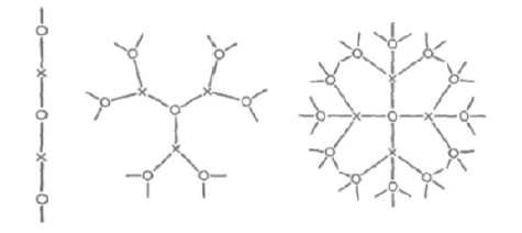
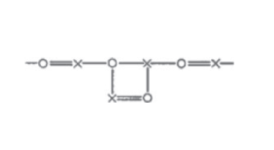
There are sections on line complexes in Nevanlinna’s book [78], in Sario and Nakai’s book [93] and in L. I. Volkovyskii’s comprehensive survey on the type problem [108]. We shall return to line complexes in §7.2.
Historical note Andreas Speiser (1885–1970) was a Swiss mathematician who studied in Göttingen, first with Minkowski and then with Hilbert. The latter became his doctoral advisor for a few months, after the death of Minkowski in 1909 (at age 44). Speiser defended his PhD thesis, in Göttingen, in 1909 and his habilitation in 1911, in Strasbourg. He worked in group theory, number theory and Riemann surfaces, and was the main editor of Euler’s Opera Omnia. He edited 11 volumes and collaborated to 26 others of this huge collection. Ahlfors writes in his comments to his Collected works [16, vol. 1, p. 84], that the type problem, which we shall review in §7, was formulated for the first time by Andreas Speiser. The latter introduced line complexes (in a version slightly different from the one we use here) in his papers [97] and [98]. In his paper [15], Ahlfors writes: “Around 1930 Speiser had devised a scheme to describe some fairly simple Riemann surfaces by means of a graph and had written about it in his semiphilosophical style”. Ahlfors adjective is related to the fact that Speiser’s articles do not contain formulae.
6.3 Thurston’s realization theorem
A branched covering from the sphere to itself can be iterated (composed with itself). The postcritical set of such a branched covering is the union of the set of critical points with its forward images by the mapping. A branched covering is said to be postcritically finite if its postcritical set is finite. In 1983, Thurston obtained a characterization of branched coverings of a topological 2-sphere that are topologically equivalent to postcritically finite rational maps of the Riemann sphere, that is, quotients of two polynomials (see [103] and the exposition in [25]). In 2010, while he was considering again the question of understanding holomorphic mappings from the topological point of view, Thurston obtained a realization theorem for branched coverings of the sphere which we present now. The result involves the Speiser graph associated with a branched covering of the sphere that we defined in §6.2. We now state this result.
Let be a generic degree branched covering of the topological sphere . Here, the word generic means that the cardinality of the set of critical values of is (which is the largest possible). This implies that the cardinality of the set of critical points is also . Every critical point of such a map is simple (of order 1).
Let be a Speiser curve associated with this covering, equipped with its orientation, and consider its lift . This is a graph we called Speiser graph. Its vertices are all of valence 4 (we do not take into account lifts of the critical values that are not critical points).
The Speiser curve divides the sphere into two connected components which are naturally equipped with polygonal structures. We color these components in blue and white. Each connected component of the complement of is sent by to a connected component of , and therefore it carries naturally a color and a polygonal structure. We call such a component a face of . Thurston addressed the following question:
To characterize the oriented 4-valent graphs in that can be obtained by the above construction, that is, as a Speiser graph associated with some branched covering .
He proved the following:
Theorem 6.2 (Thurston, see [62])
Let be an oriented graph on , with vertices, all of valence 4. Then is a Speiser graph of a degree- branched covering of the sphere onto itself if and only if:
-
1.
each face of is simply connected;
-
2.
for any alternating blue-white coloring of the faces of , there are white faces and blue faces;
-
3.
for every oriented Jordan curve embedded in and bordered by only blue faces on the left and only white faces on the right (excluding the corners), the Jordan disc bounded on the left by this curve contains strictly more blue faces than white faces.
Thurston’s proof of Theorem 6.2 given in [62] is based on the so-called “marriage theorem” (due to Philip Hall) from combinatorics, a theorem dealing with finite subsets of a given set; it gives a necessary and sufficient condition on such a family that guarantees the choice of one element from each set such that these elements are all distinct (monogamy is the rule). The authors in [62] ask for a better proof which would give an algorithm for constructing arbitrary rational functions whose critical values are on the unit circle [62, p. 255].
The Riemann–Hurwitz formula, which we recalled in §6.1, becomes in the case at hand, i.e., the case where is a degree- branched cover of the sphere by itself:
In this formula, the sum is taken as before over the critical points , and is the branching order at . (This formula follows from the fact that the Euler characteristic of both surfaces is 1.) Written in this form, the Riemann–Hurwitz formula says that the branching information at the various points forms a partition of the integer . The question of what are the partitions that are realized by a branched covering of the sphere to itself is still open. (Cases where the map does not exist are known to occur.)
Thurston’s result is part of his project of understanding the shapes of rational functions, where by “shape” he means the evolution of the critical levels of such a function (see his comments on this problem in a MathOverflow thread he started in 2010, titled What are the shapes of rational functions?).
The paper [6] which contains a stratification of spaces of monic polynomials of a give degree is inspired by Thurtson’s question. See also LABEL:BE2009
7 The type problem
The Uniformization Theorem (Theorem 5.2) says that every simply connected Riemann surface is either conformally equivalent to the Riemann sphere, or to the complex plane, or to the unit disc. In the first (respectively, second, third) case, is said to be of elliptic (respectively, parabolic, hyperbolic) type. The names stem from the fact that the Riemann sphere, the complex plane and the unit disc are ground spaces for elliptic, parabolic and hyperbolic geometry respectively (elliptic and parabolic geometries are alternative names for spherical and Euclidean geometries). The first case is distinguished from the other two by topology, since in this case is compact, whereas in the two other cases it is not.
The type problem asks for a practical way to decide whether a given simply connected non compact Riemann surface is of parabolic or elliptic type.
The answer depends on the context in which the surface is defined. For instance, the surface may be embedded in Euclidean 3-space and equipped with the induced metric, or it may be equipped with some abstract Riemannian metric, or it may be obtained by pasting smaller surfaces (Euclidean or non-Euclidean polygons, etc.). It may also be given as an infinite branched covering of the sphere with some data at each branching point, or it may be obtained by analytic continuation, like the universal cover of the Riemann surface of some holomorphic function. One can also imagine other situations. The multiplicity of these cases explains the variety of ways and techniques in which the type problem has been addressed; we shall see some examples below.
7.1 Ahlfors on the type problem
Ahlfors emphasized at several occasions the importance of the type problem, which was one of his main research topics during the period 1929–1941. In his paper [13], talking more precisely about the question of deducing the type of a Riemann surface associated with a univalent function, from the distribution of its singularities, he writes: “This problem is, or ought to be, the central problem in the theory of functions. It is evident that its complete solution would give us, at the same time, all the theorems which have a purely qualitative character on meromorphic functions.” Nevanlinna, in the introduction of his book Analytic functions (1953), ), writes (p. 1 of the English edition [78]): “[…] Value distribution theory is thus integrated into the general theory of conformal mappings. From this point of view the central problem of the former theory is the type problem, an interesting and complicated question, left open by the classical uniformization theory.”
One of Ahlfors’ earliest results on the type problem is a theorem contained in his paper [12]. It gives the following condition for a simply connected surface which is a branched covering of the sphere whose branch values are all of finite degree, to be parabolic. See also LABEL:Ahlforsthesis.
Theorem 7.1 (Ahlfors, [12])
Let be a simply connected surface which is a branched covering of the sphere with all branch values of finite degree, let be an arbitrary point in and let be a function defined on which associates with the number of branch points, counted with multiplicity, at distance from . If
for some (or equivalently for all) , then is of parabolic type.
Thus, the theorem says that if the amount of branching is relatively small, the surface is parabolic. We shall see below other results on the type of branched coverings of the sphere that are also expressed in terms of the growth of the amount of branching. Heuristically, one can consider that the degree of branching measures a certain degree of negative curvature concentrated at the branch points, and consequently, the larger the amount of branching is, the more negative curvature is concentrated at that point; this explains the fact that a surface with a large amount of branching is hyperbolic.
In the setting of function theory, one also admits branch values of infinite degree, modeled on the ones that occur in the theory of Riemann surfaces of multi-valued analytic functions. The complex logarithm function is an example of a multivalued function which gives rise to a branch value of infinite degree.
In the next 3 subsections, we shall describe different approaches used by various authors to the study of the type problem. They involve combinatorial, analytical and geometrical methods.
7.2 Nevanlinna on the type problem
Nevanlinna, in the papers [76, 77, 78] considered in detail the type problem for simply connected surfaces that are branched coverings of the sphere with a finite number of critical values. Soon after, Teichmüller dealt with the same problem in his papers [100] and [101], disproving a conjecture made by Nevanlinna. The fundamental tool that is used in these works is the line complex that we recalled in §6.2.
Nevanlinna formulated a principle which amounts to formalizing the fact that the type of a simply connected Riemann surface which is a branched covering of the Riemann sphere may be deduced from information on the associated line complex. The faces of this graph (i.e., the connected components of its complement) are in one-to-one correspondence with the branch points of the covering, if one discards bigons. A polygon with sides is associated with a branch point of order . Roughly speaking, Nevanlinna’s claim is that if the amount of branching of the covering is small, the surface is of parabolic type, and if the amount of branching is large, the surface is of hyperbolic type. He showed how the amount of branching can be deduced from the properties of the line complex. Nevanlinna writes, in [78, p. 308]: “It is thus natural to imagine the existence of a critical degree of branching that separates the more weakly branched parabolic surfaces from the more strongly branched hyperbolic surfaces.” To make this precise, he introduced the notions of mean branching and mean excess relative to the line complex. These are analogues of the notion of global mean curvature of a surface. We shall recall his definition.
To motivate the above principle, Nevanlinna first considered the case of a surface which, instead of being an infinite-sheeted covering of the Riemann sphere, is finite-sheeted. In this case, the mean branching is simply the sum of the orders of the branch points divided by the degree of the covering.
In this case, the mean branching can also be computed using the line complex . The number of vertices of the line complex is equal to twice the number of sheets. Indeed, if is the number of sheets in the covering, then, using the notation in §6.2, there are vertices which are lifts of the point and others which are lifts of the point . Each branch point of order is in the interior of a polygonal component of having sides and vertices. Considering that twice the order of this branch point, that is, , is evenly distributed among these vertices, each vertex of this polygon receives from the polygon itself a branching contribution equal to . Taking the sum over the contributions coming from all the adjacent polygons, each vertex of the line complex receives a total branching contribution equal to , where the sum is over all the polygons adjacent to this vertex. Dividing by the total number of vertices, which is twice the number of sheets, gives the mean branching. Nevanlinna uses this second way of counting the mean branching for the definition of the mean branching in the case of an infinite covering.
Nevanlinna considered first the case of a regularly ramified surface. This is a surface whose group of covering transformations acts transitively on the set of branch points (therefore it acts transitively on the line complex). In this case, the mean ramification is equal to the ramification of an arbitrary polygonal component in the complement of the line complex. He proved:
Theorem 7.2 (Nevanlinna [78], p. 311)
For a regularly ramified surface, the following holds:
-
1.
the surface is parabolic if the mean ramification is ;
-
2.
he surface is hyperbolic if the mean ramification is ;
-
3.
The surface is elliptic if the mean ramification is ;
-
Proof
In his proof, Nevanlinna introduces a metric on each polygonal component of the complement of the line complex in which the measure of the angle at each vertex of such a polygon corresponding to a branch point of order is equal to .
The excess of a polygon is equal to where is as before the cardinality of the set of critical values, which is also the number of sides of the polygon. Since we are in the case of a regularly ramified surface, the mean ramification is equal to the order of ramification at each branched point.
In case 1, the angle excess of each polygon is zero and we can realize this polygon as a regular polygon in the Euclidean plane. In case 2, the angle excess of each polygon is negative and we can realize it as a regular polygon in the hyperbolic plane. Case 3 corresponds to spherical geometry.
In the case of an infinitely-branched covering, the average of the branching over all the vertices of is obtained by taking an exhaustion of this graph by an infinite number of finite sub-graphs, and taking the lower limit of a mean of the sum of the total branchings of the vertices [78, p. 309ff]. The conjecture is formulated by Nevanlinna as a question in [78, p. 312] in the following terms: Is the surface parabolic or hyperbolic according as the mean excess is zero or negative? After formulating this question, Nevanlinna notes that Teichmüller in his paper [101], disproved the conjecture by exhibiting a hyperbolic simply connected Riemann surface branched over the sphere with a line complex whose mean excess is zero.
7.3 Quasiconformal mappings and Teichmüller’s work on the type problem
In the course of proving the above result, Teichmüller used quasiconformal mappings, and we next recall this notion.
To a differentiable complex-valued function defined on an open subset of the complex plane (or on a Riemann surface), one asssociates its complex dilatation by taking first the partial derivatives and , setting
and
and defining the complex dilatation of as
The (real) dilatation of is then given by the real function
and is said to be -quasiconformal, for some , if this function satisfies
for all in .
In practice, one allows to be only absolutely continuous on almost every line which is parallel to the real or imaginary axis. This is sufficient for the partial derivatives and to exist almost everywhere.
The dilatation is then defined a.e., and the last inequality needs only to be satisfied a.e.
A computation shows that the dilatation of at an arbitrary point is equal to the ratio of the major axis to the minor axis of the ellipses that are images by the differential of the map at that point, of circles in the tangent space centered at the origin. Therefore, a diffeomorphism between two Riemann surfaces is -quasiconformal if it takes an infinitesimal circle to an infinitesimal ellipse of eccentricity uniformly bounded by .
The map is quasiconformal if it is -quasiconformal for some finite .
This leads us to a notion of quasiconformally equivalent Riemann surfaces and quasiconformal structure, a weakening of the notion of conformal structure: A quasiconformal structure on a 2-dimensional manifold is a family of conformal structures such that the identity map between any two of them is quasiconformal. We say that two conformal structures in such a family are quasiconformally equivalent.
Teichmüller wrote a paper dedicated to applications of quasiconformal mappings the type problem, see [100], titled An application of quasiconformal mappings to the type problem. In the introduction to this paper, he writes: “Recently, the problem of determining the properties of the schlicht mapping of [a simply connected Riemann surface] from its line complex has been frequently studied. So far in the foreground has been the type problem: How can one determine, from the given line complex, if the corresponding surface can be mapped one-to-one and conformally onto the whole plane, the punctured plane, or the unit disk? One is still very far from finding sufficient and necessary conditions.”
In this work on the type problem, Teichmüller started by showing that two branched coverings of the sphere whose line complexes are equal are quasiconformally equivalent. He gave a criterion for hyperbolicity and he proved that the type of a simply connected open Riemann surface is a quasiconformal invariant [100]. The latter result is a direct consequence of the fact that the complex plane and the unit disc cannot be quasiconformally mapped onto each other, a result which he proves in the same paper. In principle, this result reduces the type problem to a simpler problem, since quasiconformal mappings exist much more abundantly than conformal mappings. To show that a surface is parabolic (respectively hyperbolic), it suffices to exhibit a quasiconformal homeomorphism between and the complex plane (respectively the unit disc).
To end this subsection on Teichmüller’s work on the type problem, let us mention the survey [17] titled Teichmüller’s work on the type problem.
7.4 Lavrentieff on the type problem
Lavrentieff’s work on the type problem is based on the notion of “almost analytic function” which he introduced, another weakening of the notion of conformal mapping which is close to (but slightly different from) the notion of quasiconformal mapping.
To state this property, let us first recall that there exist several equivalent conditions for a differentiable function from the complex plane to itself (or, more generally, between surfaces) to be holomorphic, and weakening each of them gives a weakening of a function to be holomorphic. Among these conditions, we mention the following:
-
1.
is angle-preserving.
-
2.
the real and imaginary parts of satisfy the Cauchy–Riemann equations.
-
3.
satisfies .
-
4.
The Taylor series expansion of around every point is convergent in some open disc around this point;
-
5.
The following notion of holomorphicity is stated in terms of almost complex structures: Given a surface equipped with a -holomorphic function, a differentiable function is said to be -holomorphic if for every point on and for every tangent vector at , we have
-
6.
The function possesses a complex derivative, that is, infinitesimally, it acts by multiplication by a complex number.
Lavrentieff’s almost analyticity property is a weakening of Property 6, a property equivalent to the fact that at each point the Jacobian matrix of acts on the tangent space as a rotation followed by a homothety. This is also expressed by the fact that the map sends infinitesimal circles to infinitesimal circles. (Thus, this property is close to the notion of quasiconformal mapping which we recalled in §7.2.)
In fact, in the most general case, the Jacobian matrix of a differentiable map between tangent spaces, since it acts linearly, takes circles centered at the origin to ellipses centered at the origin, and Lavrentieff’s property is formulated in terms of the boundedness of the eccentricty and the directions of these ellipses. We now state this condition in precise terms.
-
Definition
(Lavrentieff [63]) A function defined on a domain is said to be almost analytic if the following three properties hold:
-
1.
is continuous.
-
2.
is orientation-preserving and a local homeomorphism on the complement of a countable closed subset of .
-
3.
There exist two real-valued functions and , called the characteristics of , defined as follows:
-
–
There is subset of which consists of finitely many analytic arcs such that is continuous on and is continuous at each point satisfying . ( might be empty.)
-
–
On every domain whose frontier is a simple analytic curve, is uniformly continuous. Furthermore, if such a domain and its frontier do not contain any point satisfying , then is also uniformly continuous on .
-
–
For an arbitrary point in , let be an ellipse centered at , let be the angle between its major axis and the real axis of the complex plane, and let be the ratio of the major axis to its minor axis . Let and be two points on the ellipse at which the expression attains its maximum and minimum respectively. Then,
-
–
One goal of Lavrentieff’s article [63] is to show that almost analytic functions share several properties of analytic functions. This includes a compactness result for families of almost analytic functions with uniformly bounded characteristics, which is a generalization of a known compactness property that holds for families of analytic functions. It also includes a generalization of Picard’s big Theorem [63, §3]. The generalization of the same theorem for quasiconformal mappings was already obtained by Grötzsch, see [42].
The question of finding an almost analytic function from its characteristics, which Lavrentieff solves in the same paper and which we state now, is a form of what was later called the “Measurable Riemann Mapping Theorem”. This is a wide generalization of the Riemann Mapping Theorem:
Theorem 7.3 (Lavrentieff [63])
Given any two functions and defined on the closed unit disc such that and satisfy the properties in the above definition and such that for some constant , there exists an almost analytic function realizing a self-homeomorphism of the closed disc and having the characteristics and .
In the same paper, Lavrentieff proves the following result on the type problem. Like Ahlfors’ theorem (Theorem 7.1) and like the theorem of Milnor that we shall quote below (Theorem 7.5), Lavrentieff’s theorem reduces the question of proving parabolicity to that of proving that a certain integral diverges.
Theorem 7.4 (Lavrentieff [63])
Let be a surface in the 3-dimensional Euclidean space which is the graph of a differentiable function
whose partial derivatives and are continuous. For each , let
If , then is of parabolic type.
Lavrentieff, in his paper, reduced the type problem to Theorem 7.3, that is, to the problem of finding an almost analytic function having given characteristics and , such that for ,
where is the angle formed by the -plane and the tangent plane of at and where is the angle formed by and the -axis.
7.5 Milnor on the type problem
Milnor, in his paper [74], studied the type problem for the case of a surface embedded in Euclidean 3-space which is complete and whose Gaussian curvature depends only on the distance to some fixed point . The Riemannian metric induced on this surface can be written in the polar coordinates as where is a smooth positive function that denotes the length of the geodesic circle of radius centered at . The Gaussian curvature is then given by .
Milnor proves the following:
Theorem 7.5
For a surface as above we have:
-
1.
is parabolic if and only if for some (or equivalently for any) , the integral .
-
2.
If for an arbitrary we have for large enough, then is parabolic.
-
3.
For any , we have for large enough , and if the function is unbounded, then is hyperbolic.
Items 2 and 3 are not surprising if we consider them again from the point of view that enough negative curvature corresponds to a hyperbolic type and enough positive curvature corresponds to a parabolic type. An interesting fact here is that the difference between the two cases is made by an which can be chosen to be arbitrarily small, and in this sense the result is the best possible in the given situation.
-
Milnor’s proof
The proofs of Items 2 and 3 follow from Item 1 which, like the results of Ahlfors and Lavrentieff that we mentioned above, characterizes parabolicity in terms of the divergence of a certain integral.
For the proof of 1, Milnor introduces a new coordinate . In the coordinates , the metric becomes
and is thus conformally equivalent to the Euclidean metric. (Coordinates in which the metric is conformal to the Euclidean metric are called isothermal, another term which comes from the theory of heat transfer.) The exponential map maps conformally onto . (The mapping is a priori defined in the complement of the point , but it extends to because it is bounded, differentiable and conformal in a neighborhood of , therefore this singularity is removable.)
Milnor, at the end of his paper, adresses the question of finding an effective criterion for deciding, for a simply connected open surface embedded in 3-space, whether it is parabolic or hyperbolic.
7.6 Probablistic approaches
There are other approaches to the type problem that we shall not touch upon here. In particular, there is a probabilistic point of view. A classical result in this direction says that a surface equipped with a Riemannian metric is parabolic if and only if the associated Brownian motion is recurrent. There is a large literature on this question, see e.g., Kakutani’s paper [54], which appeared the same year as Teichmüller’s paper [100] on the type problem. Kakutani gives the following criterion: Let be a simply-connected open Riemann surface which is an infinite cover of the sphere and let be a simply connected subset of bounded by a Jordan curve . For a point in , let denote the probability that the Brownian motion on starting at enters into without getting out of before. Then, one of the following two cases holds:
-
1.
everywhere in and in this case is hyperbolic;
-
2.
is identically equal to 1 , and in this case is parabolic.
Let us also mention Z. Kobayashi’s papers on Riemann surfaces in which he discusses the type problem; see in particular his paper [57] in which he gives sufficient conditions under which a surface is of parabolic type, and his paper [58] in which he presents a theory based on Kakutani’s paper [54] and Teichmüller’s paper [101], generalizing both works. Figure 5 is extracted from Kobayashi’s paper [57]. It is reproduced here for the purpose of showing the nobility of this kind of drawing compared to computer-drawing everybody uses today in mathematical papers.
7.7 Electricity
P. Doyle and J. L. Snell expanded on the relation between the type problem, Brownian motion and the propagation of an electric current on the surface, see the paper [32] where the main underlying idea is that the unit disc has finite electrical resistance while the plane has infinite resistance. See also Doyle’s review in the Bulletin of the AMS, [31], in which the author reports on the type problem for a covering of the Riemann sphere with punctures using the properties of the Speiser graph of the covering, surveying the important work of Lyons–McKean–Sullivan [69] and of McKean–Sullivan [72] on this topic. Incidentally, the author seems not to be aware of the work of Teichmüller on these questions.
Introducing electricity in the type problem is completely in the tradition of Riemann who, at several places in his work on Riemann surfaces uses arguments from electricity. This occurs in particular in the two main papers where he deals with Riemann surfaces, namely, his doctoral dissertation [88] and his paper on Abelian functions [89]. For instance, in the Dirichlet principle that he used in his proof of the Riemann Mapping Theorem (see §5.3 above), Riemann considered the function defined on the boundary of the domain as a time-dependent electrical potential, and his conclusion in the solution to the Dirichlet problem consisted in letting the system evolve and reach an equilibrium state. The function obtained necessarily satisfies a mean value property and therefore is harmonic.
Historical note In the summer of 1858, Riemann gave a course titled The mathematical theory of gravitation, electricity and magnetism [91]. Besides his mathematical papers in which he used electricity, Riemann also wrote papers on electricity. See his unfinished paper Gleichgewicht der Electricität auf Cylindern mit kreisförmigen Querschnitt und parallelen Axen (On the equilibrium of electricity on cylinders with circular transverse section and whose axes are parallel) [87] (1857) published posthumously in the second edition of his Collected works which concerns the distribution of electricity or temperature on infinite cylindrical conductors with parallel generatrices. The reader interested in more details may refer to the survey titled Physics in Riemann’s mathematical papers [79].
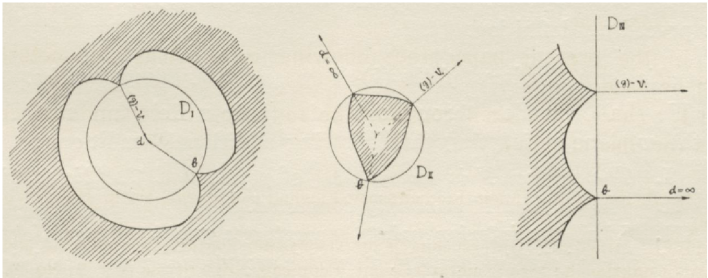
-
Remark
(Higher-dimensional generalizations) One advantage of introducing random walks and probabilistic methods in the theory of parabolicity/hyperbolicity of Riemann surfaces is that it allows this theory to be generalized to graphs, discrete groups and higher-dimensional manifolds. There are several works in this direction. I mention Marc Troyanov’s paper [105] in which he discusses parabolicity for -dimensional manifolds. More precisely, in this paper, Troyanov surveys an invariant of Riemannian manifolds which is related to the non-linear potential theory of the -Laplacian and which determines a property which generalizes parabolicity or hyperbolicity of surfaces. The key notion that this leads to is that of -parabolicity and -hyperbolicity. In the generalized setting of the paper [105], the classical dichotomy parabolic/hyperbolic becomes -parabolic/-hyperbolic, i.e., . The author focuses in particular on the relationship between the asymptotic geometry of a manifold and its parabolicity.
8 Uniformization: Geometry and combinatorics
8.1 Dessins d’enfants
A map on a compact oriented surface is a bicolored finite graph embedded in such that each connected component of is contractible. The vertices of the graph are colored by and each edge joins vertices of different colors. A connected component of is called a cell of the map. A map can be upgraded to a triangulation by choosing a point in each cell and connecting the chosen point by a star-shaped system of curves to the vertices of that are on the boundary of the cell. The triangulation is special in that it admits a checkerboard black-white coloring (that is, triangles meeting from opposite sides along an edge have opposite colors). To see this, we use the symbols to color the vertices of the triangulation in such a way that the chosen points in the cell gets the color . Each triangle has vertices of different colors, hence becomes oriented by imposing the cyclic order . Finally we color white those triangles for which the induced orientation from coincides with the cyclic orientation of the vertices.
The minimal example of a map is . Here, the graph is with two vertices and one edge embedded in the Riemann sphere . This map has only one cell. Now choose the point connected by and as an upgrading to a triangulation with two triangles, the white one being the so-called upper half-plane . We denote by this minimal map together with the above upgrading to a triangulation.
Speiser graphs discussed in §6.2 are maps in the above sense, except that the surfaces on which they are defined are not necessarily compact.
Let it be given the combinatorial data consisting of a triple of a map with its bicoloring on a compact surface , together with the upgrading to a checkerboard colored triangulation .
A smooth mapping is well defined up to isotopy. It sends vertices to vertices respecting colors, edges to edges, and its restriction to the complement of the vertex set of the triangulation is a submersion.
Let be the complex structure on obtained by pulling back the complex structure of and by extending this structure using the removable singularity theorem.
The result is again an upgrading from the combinatorial data to a Riemann surface together with a holomorphic function having its critical values in the set .
The set of possible combinatorial data up to isotopy is countable and the set of Riemann surfaces up to bi-holomorphic equivalence is uncountable. Thus, a natural question arises, namely, what Riemann surfaces appear as an upgrading of a map. The answer is given by Belyi’s Theorem:
Theorem 8.1 (Belyi [19])
For a compact Riemann surface the following are equivalent:
-
1.
carries a holomorphic map with at most critical values (which can be taken, without loss of generality, to be );
-
2.
is bi-holomorphically equivalent to an upgraded map surface;
-
3.
is bi-holomorphically equivalent to a complex curve, that is, a Riemann surface embedded in the projective space defined by a set of polynomials with coefficients in a number field, that is, a finite field extension of the field of rational numbers.
The implication is the “easy part”; indeed, the inclusion as an algebraic curve defined by a set of polynomials with coefficients in a number field can be composed (with care) with projections to lower-dimensional spaces until one gets a meromorphic function on . Using the fact that this function is itself defined on a number field, there is a way of reducting the number of critical values to at most three.
The strength of Belyi’s Theorem can already be appreciated in the case of genus surfaces and maps having only one cell, or, equivalently, in the case where the graph is a planar tree in the Gaussian plane . The above construction leads in this case of a map to a polynomial having at most two critical values. Such a polynomial becomes well defined if one marks an edge of and requires that sends its extremities to .
The study of polynomial mappings with at most two critical values was introduced by G. Shabat, see [95] and [96]. These polynomials generalize Chebyshev polynomials which have only two critical values and such that these critical points are all of Morse type. Equivalently, there is a maximal number of such critical points.
This fact leads to an action of the absolute Galois group on the set of isotopy classes of bicolored planar trees with marked edges. This action is faithful and a window for observing and perhaps understanding the absolute Galois group. See Geothendieck’s Sketch of a program [40]. We also refer to the review made in [10] of the relevant parts of the Esquisse.
The inverse image of the interval by may look like a drawing of a person by a child, hence the name “dessin d’enfants” given by Grothendieck to this mathematical object whose study he promoted in [40]. For an introduction to dessins d’enfants we refer to the original article [40] and to the expositions in [38, 43, 47]. The reader interested in the relation between dessins d’enfants and the deformation theory of Riemann surfaces may refer to [46].
Voevodsky and Shabat in [107] considered surfaces equipped with Euclidean structures with cone singularities obtained by gluing Euclidean equilateral triangles along their sides. They showed that the Riemann surface structure underlying such a metric space, as an algebraic curve, is defined over a number field. Cohen, Itzykson and Wolfart in [27] showed that the same construction works using congruent hyperbolic triangles (triangles in the Bolyai–Lobachevsky plane), instead of Euclidean.
8.2 Slalom polynomials
We shall use the notions of slalom polynomial and slalom curve and we shall recall the definitions. For a more detailed exposition we refer to the original article [4] and the recent book [8] by the first author.
We start with the definition of the planar tree associated with a generic monic polynomial of degree . This is the closure of the union of the flowlines of that satisfy the following properties:
-
•
and its derivative do not vanish on the image of ;
-
•
the image of is maximal with respect to inclusion (in other words, is not the restriction of a flowline defined on an interval strictly containing );
-
•
the image of is bounded in , except when is the positive real line and where this image converges to .
Consider now a rooted planar tree with edges in which one vertex is connected to (considered as the root) by an unbounded edge. A slalom curve of is an immersed copy of the circle having transversal double points at the midpoints of the bounded edges of (Figure 6). The curve intersects only and transversely twice at the midpoints of the bounded edges and once at the unbounded edge such that each bounded complementary region of the curve contains exactly one vertex.
A slalom polynomial for is a generic monic polynomial of degree with for each zero of such that the colored trees and are isotopic relative to . Generic means in this context that has distinct roots, and that has distinct roots.
A slalom polynomial is a generic monic polynomial that is a slalom polynomial for some tree .
Slalom polynomials share the following properties with Shabat and Chebyshev polynomials: has distinct roots and all critical values of have absolute value . Thus, the roots of are the double points of the curve , which is a slalom curve for the tree .
Theorem 8.2 (Existence of slalom polynomials)
Given a rooted planar tree with edges as above, there exists a slalom polynomial for .
- Proof
There exists a continuous mapping that is smooth except at the midpoints of and such that
-
–
the restriction of to the unbounded component of the complement of is a degree covering map of the complement of the closed unit disc in ;
-
–
the restriction of to a bounded region of the complement of is a diffeomorphism to the open unit disc in that sends the vertex to and half edges to radial rays;
-
–
is holomorphic near .
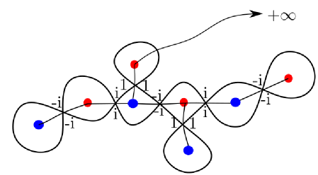
Let be the conformal structure on such that is holomorphic and let be a uniformisation of the structure . The composition is a degree polynomial. The polynomial has roots, the derivative has roots at the points with being a midpoint of an edge. By adjusting the uniformisation map one achieves that is monic and generic.
The flowline from ends at a root of that we color red and which becomes the root of . This red root can be changed by substituting to . This substitution turns the picture and gives possibilities for attaching the unbounded edge. Color the tree with the two colors, red and blue. Choose a disc that contains up to a part of the real axis.
It follows that and are isotopic relative to , showing that all the combinatorial data consisting of a rooted planar tree as above are realized. Here designates the -th Catalan number, that is, the number of distinct triangulations of a convex polygon with sides obtained by adding diagonals.
The polynomial is a slalom polynomial for the tree .
The slalom polynomial is not unique up to holomorphic changes of coordinates in the range and in the target. Uniqueness can be forced for trees with maximum valence if one imposes moreover that the critical values are roots of unity of order depending on . See Figure 6. For , order four works. In Figure 6, the values are the values of the polynomial at the given points.
In the example of Figure 7, the polynomial is the slalom polynomial of the tree . The Chebyshev polynomials are up to a real translation precisely the slalom polynomials with critical values among . See also [7].
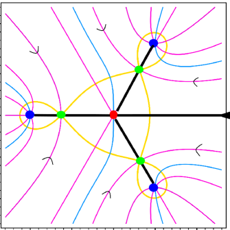
As in [6] one obtains a cell-decomposition of the space of monic polynomials of degree and of the complement of the discriminant (the set of polynomials having at least one multiple root).
Theorem 8.3
The equivalence relation induces a stratification with top-dimensional strata on the spaces and . Moreover, the top-dimensional strata are cells and have a representative by a slalom polynomial.
For this theorem, see [7].
8.3 A stratification of the space of monic polynomials
The space of monic univariate complex polynomials of degree is a complex affine space of dimension . The discriminant is an important sub-variety. A cell decomposition of that induces a cell decomposition of is of interest, for instance in the study of the braid group. The following defines an equivalence relation on , whose associated equivalence classes define a cell decomposition such that the discriminant is a union of cells, see [6].
Define the picture of a monic polynomial to be the graph . Call two polynomials equivalent if the graphs and are isotopic by an isotopy that preserves the asymptotes.
The picture of a degree monic polynomial is a planar forest without terminal vertices, but with edges going to asymptotic to the rays corresponding to roots of unity. The precise combinatorial characterization is given in [6]. The problem of showing that each possible equivalence class is realized was solved using Riemann’s Uniformisation Theorem. The number of top-dimensional cells is the Fuss–Catalan number .
8.4 Rational maps, Speiser colored cell decompositions, classical knots and links.
Let be a holomorphic map of degree . Such a map is also called a rational map, since in the above coordinate its expression is a ratio of two polynomials of degrees with .
Let be the finite set of critical values of . The restriction of to the complement of the set is a covering map of degree . The set contains the set of critical points of . For each , define the defect by . Observe that except for . The Riemann–Hurwitz formula becomes here
as follows from computing the Euler characteristic of the domain of ,
Let be the number of critical values of . Clearly, . Recall (§6.2) that a Speiser curve for is an oriented simple closed smooth curve in that passes through all the critical values . Observe that two such curves are smoothly isotopic, keeping fixed, if and only if the induced cyclic order on the elements of agree. So up to isotopy one has isotopy classes of curves through the points of . A Shabat polynomial or a Belyi map with three real critical values admits up to isotopy two Speiser curves, one being .
From a Speiser curve one constructs the Speiser graph as the pair in . The vertices are colored by the elements of the branching set and the edges are oriented by lifting the orientation of . The Speiser curve being smooth, the curve is the image of the immersion of finitely many copies of ( denotes disjoint union). The immersion has no tangencies and equi-angular multiple points at the critical points of (see Figure 8). Each complementary region of is a polygon with vertices. We color such a polygon by : by only if the induced orientation on agrees with the orientation of , in which case the colors of the vertices of appear in the cyclic order induced by . The coloring of the polygons is a checkerboard coloring.
The Speiser graph is in fact an immersion of circles without tangencies in . The immersion is not a generic immersion, since self-intersection of or more local branches occur. But, at all self-intersections the local branches intersect pairwise transversely.
We recall that a divide in the sense of [3, 5] is the image of a relative generic immersion of a finite union of copies of the unit interval in the unit disc . From a divide , one defines a link in by
where the 3-sphere is seen here as the unit sphere in the tangent bundle of .
By a result of [3], if the image of the immersion defining a divide is connected, then the associated link is fibered. The theory of links associated with divides is closely related to singularity theory [2, 45]. In the paper [3], the monodromy of the fibered link associated with a connected divide is described in terms of the combinatorics of the divide.
Many constructions for divides still apply to Speiser graphs.
Let be the set of length tangent vectors to the Speiser graph. Let be the set of oriented length tangent vectors to .
Recall that the 3-sphere and the Lie group are diffeomorphic and cover by a map the space of length tangent vectors to . Hence and can be considered as subsets in and lift to the classical knots and links in , which we call Speiser links. See Figure 8 for an example of a Speiser graph and 9 for its Speiser link.
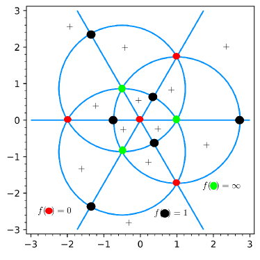
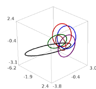
Theorem 8.4
The subsets and are links in . The lifts to are classical links. Moreover, the link is fibered.
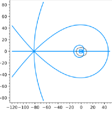
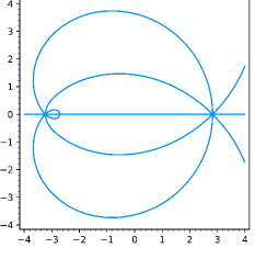
-
Proof
Let be a continuous oriented vector field of length along . Each component of together with the restriction of the vector field lifts by to smooth arcs in . The lifted arcs are pairwise disjoint. At a critical point of , arcs join. The local germ of at is diffeomorphic to the germ at of the set . So, after a small perturbation of locally near the critical points of , the graph can be deformed to a divide with checkerboard coloring on . The connected components of the complement are contractible and moreover has no self-intersection other than double points. The construction in [3] associates the knot or link in . The fibration property as in [3] was extended by Masaharu Ishikawa and Hironobu Naoe [49, 48] and shows that is a fibered knot or link in . The same holds for its lift and also the link .
The construction of the fiber surface and geometric monodromy for the link as in [3] is as follows. Let be a small -deformation of with only double points. The links and are isotopic, hence equivalent as links. The main step in the construction is the choice of a Morse function having one maximum in each -region, one minimum in each -region, and as critical level through all saddle points. Define . The closure of in is a surface with boundary spanning the link . The lift is a spanning surface and its interior a fiber surface for the link .
On the surface appears a system of simple closed curves: for each maximum of the circle of length tangent vectors in the kernel of , each gradient line of that connects a maximum to a minimum through a saddle point of lifts to a simple closed curve on , and to each minimum of corresponds a simple closed curve built with pieces from preceding ones, see [3]. The monodromy is a composition of the positive Dehn twists along these curves.
The examples of Belyi maps are taken from the papers of K. Filom [34] and K. Filom and A. Kamalinejad [35] in which dessins on modular curves are computed, studied and used. In the first example the divide is the union of Moebius circles, which is not always the case. More complex components can appear as the second example shows.
The link of a rational Belyi map where the Speiser curve can be given as follows explicitly as the closure in of the set
which is the union of smooth arcs, .
The tangential lift of an oriented Moebius circle on to is an oriented great circle on . Indeed, by the isometric action, move to be the parametrized curve . The curve on given by
is its lift. From follows the claim.
Let be closed disks in having as oriented boundary the Moebius circles . If are complementary, the circles differ only by orientation as do their lifts. If the boundaries of touch tangentially in one point, the lifts intersect in two points. If the intersection is open, then the lifts are disjoint great circles.
Orient as the boundary of the unit ball in . Assume that are disjoint, so that the boundaries of are disjoint or meet in two points. The linking number of the lifts of the oriented boundaries is given by .
In our example above with great circles as lifts, all pairwise linking numbers are equal to .
Acknowledgement Part of this survey is a revision of notes for lectures that were given by the first author at a CIMPA school in Varanasi (India), in December 2019. The authors would like to thank Bankteshwar Tiwari, the local organiser of this school, for his care and his excellent management. The second author is supported by the lnterdisciplinary Thematic lnstitute CREAA, as part of the ITl 2021-2028 program of the University of Strasbourg, CNRS and Inserm (ldEx Unistra ANR-10-IDEX-0002), and the French lnvestments for the Future Program.
References
- [1] J. F. Adams, Vector fields on spheres, Ann. of Math. (2) 75 (1962), 603-632.
- [2] N. A’Campo, Le groupe de monodromie du déploiement des singularités isolées de courbes planes. II. Proceedings of the International Congress of Mathematicians (Vancouver, B. C., 1974), Vol. 1, p. 395-404. Canad. Math. Congress, Montreal, Que., 1975.
- [3] N. A’Campo, Generic immersions of curves, knots, monodromy and gordian number, Inst. Hautes Études Sci. Publ. Math. 88 (1998), 151-169.
- [4] N. A’Campo, Planar trees, slalom curves and hyperbolic knots. Inst. Hautes Études Sci. Publ. Math. No. 88 (1998), 171-180.
- [5] N. A’Campo, Real deformations and complex topology of plane curve singularities, Ann. Fac. Sc. Toulouse, Mathématique, Série 6, t. 8 (1999) no. 1, p. 5-23.
- [6] N. A’Campo, Signatures of polynomials, in: In the tradition of Thurston: Geometry and Topology (K. Ohshika and A. Papadopoulos, ed.), Springer Verlag, 2020, p. 527-543.
- [7] N. A’Campo, Flowbox decomposition for gradients of univariate polynomials, billiards, treelike configurations of vanishing cycles for curve singularities and geometric cluster monodromy group, EMS Surv. Math. Sci. 9, No. 2, 389-414 (2022).
- [8] N. A’Campo, Topological, differential and conformal geometry of surfaces, Universitext, Springer, 2021.
- [9] N. A’Campo, A. Papadopoulos, Notes on hyperbolic geometry, in: Strasbourg Master class on Geometry (ed. A. Papadopoulos), pp. 1-182, IRMA Lectures in Mathematics and Theoretical Physics, Vol. 18, Zürich, European Mathematical Society (EMS), 2012.
- [10] N. A’Campo, L. Ji and A. Papadopoulos, Actions of the absolute Galois group Handbook of Teichmüler theory. Vol. IV (ed. A. Papadopoulos), Eur. Math. Soc., Zürich, 2016, p. 397-435,
- [11] L. V. Ahlfors, Üntersuchungen zur Theorie der konformen Abbildung und der ganzen Funktionen. Acta Soc. Sci. Fenn., Nov. Ser. A1 9 (1930), 1-40. In Collected works, Vol. I, 18-55.
- [12] L. Ahlfors, Zur Bestimmung des Typus einer Riemannschen Fläche, Comment. Math. Helv. 3 (1931), no. 1, 173-177.
- [13] L. V. Ahlfors, Quelques propriétés des surfaces de Riemann correspondant aux fonctions méromorphes. Bulletin de la S. M. F. 60 (1932) 197-207.
- [14] L. V. Ahlfors, Conformal invariants: Topics in geometric function theory, AMS, Rhode Island, 1973.
- [15] L. V. Ahlfors, Riemann surfaces and small point sets, Annales Academiæ Scientiarum Fennicæ, Series A. I. Mathematica, Volumen 7, 1982, 49-57
- [16] L. V. Ahlfors, Collected works, in 2 volumes, Series: Contemporary Mathematicians Ser., Birkäuser, Boston-Basel-Stuttgart, 1982.
- [17] V. Alberge, M. Brakalova-Trevithick and A. Papadopoulos, Teichmüller’s work on the type problem. In: Handbook of Teichmüller theory (A. Papadopoulos, ed.). Volume VII. Berlin, European Mathematical Society, IRMA Lect. Math. Theor. Phys. 30, 543-560 (2020).
- [18] F. Bergeron, Combinatorial Cellular Decompositions for the space of Complex Coefficient Polynomials, arXiv:0901.4020.
- [19] G. V. Belyi, Galois extensions of a maximal cyclotomic field, Izv. Akad. Nauk SSSR Ser. Mat. 43 (1979), 267-276. English transl. Math. USSR-Izv. 14 (1980), 247-256.
- [20] G. A. Belyi, Galois extensions of a maximal cyclotomic field. Math. (Translated by Neal Koblitz) USSR Izv. 14 (1980) (2): 247-256.
- [21] J. Blanc, Groupes de Cremona, connexité et simplicité, Ann. Sc. Éc. Norm. Supér. (4) 43 (2010), No. 2, 357-364.
- [22] J. Blanc, S. Zimmermann, Susanna, Topological simplicity of the Cremona groups, Amer. J. Math. 140 (2018), no. 5, 1297-1309.
- [23] P. L. Bowers, Combinatorics encoding geometry: The legacy of Bill Thurston in the story of one theorem. In In the tradition of Thurston (V. Alberge, K. Ohshika and A. Papadopoulos, eds.), Springer Verlag, 2020, p. 173-239.
- [24] W. Brägger, Kreispackungen und Triangulierungen, Enseign. Math. (2) 38 (1992), no. 3-4, 201-217.
- [25] X. Buff, G. Cui, and L. Tan, Teichmüller spaces and holomorphic dynamics. Handbook of Teichmüler theory. Vol. IV (ed. A. Papadopoulos), Eur. Math. Soc., Zürich, 2014, p. 717-756,
- [26] S. Cantat, S. Lamy, Y. de Cornulier, Normal subgroups in the Cremona group. Acta Math. 210, No. 1, 31-94 (2013).
- [27] P. Cohen, C. Itzykson and J. Wolfart, Fuchsian triangle groups and Grothendieck dessins. Variations on a theme of Belyi. Comm. Math. Phys. 163 (1994), no. 3, 605-627.
- [28] A. Connes, C. Consani and M. Marcolli, Fun with , Journal of Number Theory 129 (2009), Issue 6, p. 1532-1561
- [29] G. Darboux, Sur le problème de Pfaff, Bulletin des Sciences Mathématiques et Astronomiques, Série 2, Tome 6 (1882) no. 1, pp. 14-36.
- [30] J. Déserti, The Cremona group and its subgroups, Mathematical Surveys and Monographs 252. Providence, RI: American Mathematical Society, 2021.
- [31] Random walk on the Speiser graph of a Riemann surface. Bull. Am. Math. Soc., New Ser. 11 (1984), 371-377.
- [32] P. Doyle and J. L. Snell, Random walks and electric networks. The Carus Mathematical Monographs, Volume 22, American Mathematical Society, 1984.
- [33] C. Ehresmann, Sur les variétés presque complexes, Proc. Internat. Congr. Math. (Cambridge, Mass., Aug. 30-Sept. 6, 1950) 2, p. 412-419 (1952).
- [34] K. Filom, The Belyi characterization of a class of modular curves, J. Théor. Nombres Bordeaux 30 (2018), no. 2, 409-429.
- [35] K. Filom and A. Kamalinejad, Dessins on Modular Curves, arXiv:1603.01693.
- [36] P. Fatou, Séries trigonométriques et séries de Taylor, Acta Math., 30 (1966), p. 335-400.
- [37] D. Gabai, The Whitehead manifold is a union of two Euclidean spaces. Journal of Topology. 4 (2011) (3), 529-534.
- [38] G. Girondo, G. González-Diez, Introduction to compact Riemann surfaces and dessins d’enfants, London Mathematical Society Student Texts, 79, Cambridge University Press, 2012.
- [39] J. W. Gray, Some global properties of contact structures, Ann. of Math., 69, 2 (1959), 421-450.
- [40] A. Grothendieck, Esquisse d’un programme, Unpublished manuscript (1984). English translation: Sketch of a program, in: Geometric Galois actions, 1, London Math. Soc. Lecture Notes Ser., Vol. 242, Cambridge Univ. Press, Cambridge, 1997, p. 5-48.
- [41] H. Grötzsch, Über einige Extremalprobleme der konformen Abbildung. Ber. Verhandl. Sächs. Akad. Wiss. Leipzig Math.-Phys. Kl. 80 (1928), 367-376. English translation by A. A’Campo-Neuen, On some extremal problems of conformal mappings. In Handbook of Teichmüller theory, Volume VII (A. Papadopoulos, ed.), EMS Publishing House, Zürich, 2020, p. 355-363.
- [42] H. Grötzsch,Über die Verzerrung bei schlichten nichtkonformen Abbildungen and über eine damit zusammenhängende Erweiterung des Picardschen Satzes. Ber. Verhandl. Sächs. Akad. Wiss. Leipzig Math.-Phys. Kl. 80 (1928), 503-507. English translation by M. Brakalova-Trevithick, On the distortion of schlicht non-conformal mappings and on a related extension of Picard’s theorem. In Handbook of Teichmüller theory (A. Papadopoulos, ed.), Volume VII, EMS Publishing House, Zürich, 2020, p. 371-374.
- [43] P. Guillot, A primer on dessins. Handbook of Teichmüller theory. Vol. VI (ed. A. Papadopoulos), Eur. Math. Soc., Zürich, 2016, p. 437-466.
- [44] M. Gromov, Pseudo-holomorphic curves in symplectic manifolds. Inventiones Mathematicae, 82 (1985), p. 307-347.
- [45] S. M. Gusein Zade, Dynkin diagrams for singularities of functions of two variables. Funct. Anal. Appl. 8, 10-13 (1974) and Funct. Anal. Appl. 8, 295-300 (1974).
- [46] W. J. Harvey, Teichmüller spaces, triangle groups and Grothendieck dessins. Handbook of Teichmüller theory. Vol. I, 249-292, IRMA Lect. Math. Theor. Phys., 11, Eur. Math. Soc., Zürich, 2007.
- [47] F. Herrlich and G. Schmithüsen, Dessins d’enfants and origami curves. Handbook of Teichmüller theory. Vol. II (ed. A. Papadopoulos), Eur. Math. Soc., Zürich, 2009, p. 767-809.
- [48] M. Ishikawa, H. Naoe: Milnor fibration, A’Campo’s divide and Turaev’s shadow, Singularities, Kagoshima 2017, Proceedings of the 5th Franco-Japanese-Vietnamese Symposium on Singularities, World Scientific Publishing, 2020, pp. 71-93.
- [49] M. Ishikawa: Tangent circle bundles admit positive open book decompositions along arbitrary links, Topology 43 (2004), 215-232.
- [50] G. Julia, Leçons sur la représentation conforme des aires simplement connexes, Paris, Gauthier-Villars, 1950.
- [51] S. Kakutani, Applications of the theory of pseudoregular functions to the type-problem of Riemann surface. Jap. J. Math. 13 (1937), 375-392.
- [52] S. Kakutani, Two-dimensional Brownian motion and harmonic functions. Proc. Imp. Acad. Tokyo 20 (1944), 706-714.
- [53] S. Kakutani, Two-dimensional Brownian motion and the type problem of Riemann surfaces. Proc. Japan Acad. 21 (1945), 138-140.
- [54] S. Kakutani, Random walk and the type problem of Riemann surfaces, In Contributions to the theory of Riemann surfaces, pp. 95-101. Annals of Mathematics Studies, no. 30. Princeton University Press, Princeton, N. J., 1953, p. 95-101.
- [55] A. Kirchhoff, Sur l’existence de certains champs tensoriels sur les sphères, Comptes Rendus Acad. Sc. Paris, t. 225 (1947), p. 1258-1260.
- [56] A. Kirchhoff, Beiträge zur topologischen linearen Algebra, Compositio Math. 11 (1953), 1-36.
- [57] Z. Kobayashi, Theorems on the conformal representation of Riemann surfaces. Sci. Rep. Tokyo Bunrika Daigaku, Sec. A 39 (1935), p. 125-165.
- [58] Z. Kobayashi, On Kakutani’s theory of Riemann surfaces. Sci. Rep. Tokyo Bunrika Daigaku, Sec. A 76 (1940), p. 9-44.
- [59] P. Koebe, Abhandlungen zur Theorie der konformen Abbikdung. IV Abbildung mehrfacht zusammenhängender schlichter Bereiche auf Schlitzbereiche. Acta Math. 41 (1918), 305-344.
- [60] P. Koebe, Abhandlungen zur Theorie der konformen Abbikdung. V Abbildung mehrfacht zusammenhängender schlichter Bereiche auf Schlitzbereiche (Fortsetzung). Math. Z. 2 (1918), 198-236.
- [61] P. Koebe, Über die Uniformisierung beliebiger analytischer Kurven (Dritte Mitteilung). Nachr. Ges. Wiss. Gött., Math.-Ph. Kl. (1908), 337-358.
- [62] S. Koch and L. Tan, On balanced planar graphs, following W. Thurston. In What’s next? The mathematical legacy of William P. Thurston. Ed. D. P. Thurston, Annals of Mathematics Studies 205, Princeton University Press, Princeton, NJ, 215-232 (2020).
- [63] M. A. Lavrentieff, Sur une classe de représentations continues. Mat. Sb. 42 (1935), 407-423. On a class of continuous representations, English translation by V. Alberge and A. Papadopoulos, In Handbook of Teichmüller Theory (A. Papadopoulos, ed.), Volume VII, EMS Publishing House, Berlin, 2020, p. 417-439
- [64] M. A. Lavrentieff, Sur les fonctions d’une variable complexe représentables par des séries de Riemann, Paris, Hermann, 1936.
- [65] Lázaro O. Rodríguez Díaz, A note on Kirchhoff’s theorem for almost complex spheres I, arXiv:1804.05794.
- [66] O. Lehto and L. Virtanen, Quasiconformal mappings in the plane, Springer-Verlag, New York Heidelberg Berlin 1973. English translation of the book Quasikonforme Abhildungen, Springer-Verlag, New York, Heidelberg, Berlin.
- [67] Leonardo da Vinci, The Notebooks of Leonardo da Vinci, Vol. 1, Dover, New York, 1970.
- [68] N. Lusin and J. Priwaloff, Sur l’unicité et la multiplicité des fonctions analytiques, Annales scientifiques de l’École Normale Supérieure, Série 3, Tome 42 (1925), p. 143-191.
- [69] T. J. Lyons and H. P. McKean, Jr., Winding of the plane Brownian motion, Adv. in Math. 5 1 (1984), 212-225.
- [70] Y. I. Manin Lectures on zeta functions and motives (according to Deninger and Kurokawa), Columbia University Number Theory Seminar, New York, 1992, Astérisque, 228 (4) (1995), p. 121-163.
- [71] D. McDuff and D. Salamon, Introduction to Symplectic Topology, Oxford Mathematical Monographs, 2nd edition, Oxford Univ. Press, 1998.
- [72] H. P. McKean Jr. and D. Sullivan, Brownian motion and harmonie functions on the class surface of the thrice-punctured sphere, Adv. in Math. 5 1 (1984), 203-211.
- [73] J. W. Milnor, On manifolds homeomorphic to the 7-sphere, Ann. of Math., vol. 64, no 2 (1956), p. 399-405.
- [74] J. W. Milnor, On deciding whether a surface is parabolic or hyperbolic. Amer. Math. Monthly 84 (1977), no. 1, 43-46.
- [75] J. Moser On the Volume Elements on a Manifold, Transactions of the AMS, 120 (1965) (2), 286-294.
- [76] R. Nevanlinna, Über die Riemannsche Fläche einer analytischen Funktion. In Proceedings of the International Congress of Mathematicians, Zürich, 1932, 221-239.
- [77] R. Nevanlinna, Über Riemannsche Fläche mit endlich vielen Windunspunkten. Acta Math. 58 (1932), 295-373.
- [78] R. Nevanlinna, Eindeutige analytische Funktionen, Springer Verlag, Berlin, 1953. English tr. by Ph. Emig. Die Grundlehren der mathematischen Wissenschaften. Vol. 162. Springer Verlag, Berlin-Heidelberg-New York, 1970.
- [79] A. Papadopoulos, Physics in Riemann’s mathematical papers. In From Riemann to differential geometry and relativity (L. Ji, A. Papadopoulos and S. Yamada, eds.), Springer, Berlin 2017, 151-207.
- [80] E. Pervova and C. Petronio, On the existence of branched coverings between surfaces with prescribed branch data, I, Algebr. Geom. Topol. 6 (2006), 1957-1985.
- [81] E. Pervova and C. Petronio, On the existence of branched coverings between surfaces with prescribed branch data. II. J. Knot Theory Ramifications 17 (2008), no. 7, 787-816.
- [82] S. MacLane The genesis of mathematical structures, as exemplified in the work of Charles Ehresmann, Cahiers de topologie et géométrie différentielle catégoriques, tome 21, no 4 (1980), p. 353-365.
- [83] R. Rashed and A. Papadopoulos, On Menelaus’ Spherics III.5 in Arabic mathematics, I: Ibn ‘Irāq, Arabic Science and Philosophy, vol. 24 (2014), p. 1-68.
- [84] R. Rashed and A. Papadopoulos, On Menelaus’ Spherics III.5 in Arabic mathematics, II: Naṣīr al-Dīn al-Ṭūsī and Ibn Abī Jarrāda, Arabic Science and Philosophy, vol. 25 (2015), p. 1-32.
- [85] R. Rashed and A. Papadopoulos, Menelaus’ Spherics. Early Translation and al-Māhānī/al-Harawī’s Version. De Gruyter, Scientia Graeco-Arabica 21, 2018.
- [86] F. and M. Riesz, Über die Randwerte einer analytischen Funktion Quatrième Congrès des Mathématiciens Scandinaves, Stockholm 1916, Uppsala, Almqvist, 1920, 1920, p. 27-44.
- [87] B. Riemann, Gleichgewicht der Electricität auf Cylindern mit kreisförmigen Querschnitt und parallelen Axen, Conforme Abbildung von durch Kreise begrenzten Figuren, Nachlass XXVI, 1857, In: Ges. math. Werke, 472-476.
- [88] B. Riemann, Grundlagen für eine allgemeine Theorie der Functionen einer veränderlichen complexen Grösse, (Göttingen, 1851), in: Gesammelte mathematische Werke, wissenschaftlicher Nachlass und Nachträge. Nach der Ausgabe von Heinrich Weber und Richard Dedekind neu herausgegeben von Raghavan Narasimhan. Teubner Verlagsgesellschaft, Leipzig, 1862; Springer-Verlag, Berlin (1990) p. 3-48
- [89] B. Riemann, Theorie der Abel’schen Functionen. Journal für die reine undangewandte Mathematik, 54, 115-155 (1857). In Gesammelte mathematische Werke, wissenschaftlicher Nachlass und Nachträge. Nach der Ausgabe von Heinrich Weber und Richard Dedekind neu herausgegeben von Raghavan Narasimhan.Teubner Verlagsgesellschaft, Leipzig, 1862; Springer-Verlag, Berlin (1990) p. 88-144.
- [90] D. Roy, On the paths of steepest descent for the norm of a one variable complex polynomial, arXiv:2010.01583, 2020.
- [91] E. Sellien, Notes on Riemann’s courses Themathematical theory of electricity andmagnetism and Selected physical problems of summer 1858. Nachlass Riemann. Handschriftenabteilung der Staats- und Universitätsbibliothek Göttingen. Riemann papers. Cod. Ms. B. Riemann 45, Blatt 1-23, 1858
- [92] Henri Paul de Saint-Gervais (pseudonym for a collective book), Uniformisation des surfaces de Riemann : Retour sur un théorème centenaire, ENS Editions, 2010. English translation by R. G. Burns, Uniformization of Riemann surfaces. Revisiting a hundred-year-old theorem. Heritage of European Mathematics. Zürich, European Mathematical Society, 2016.
- [93] L. Sario and M. Nakai, Classification Theory of Riemann Surfaces, Springer-Verlag, 1970.
- [94] J.-P. Serre, Le groupe de Cremona et ses sous-groupes finis, Séminaire Bourbaki, Vol. 2008/2009. Exposés 997-1011. Astérisque 332, 75-100, Exp. No. 1000 Paris: Société Mathématique de France, 2010.
- [95] G. B. Shabat and V. A. Voevodsky, Drawing curves over number fields. In The Grothendieck Festschrift, Vol. III, Progr. Math. 88, Birkhäuser, Boston 1990, 199-227.
- [96] G. Shabat and A. Zvonkin, Plane trees and algebraic numbers, In Jerusalem combinatorics, ’93, volume 178, Contemp. Math., p. 233-275. Amer. Math. Soc., Providence, RI, 1994.
- [97] A. Speiser, Probleme aus dem Gebiet der ganzen transzendenten Funktionen. Comment. Math. Helv. 1 (1929), no. 1, 289-312.
- [98] A. Speiser, Über Riemannsche Flaechen, Comm. Math. Helvetici 2 (1930), p. 284-293.
- [99] S. Stoïlov, Leçons sur les principes topologiques de la théorie des fonctions analytiques, Gauthier-Villars, Paris, 1956.
- [100] O. Teichmüller, Eine Anwendung quasikonformer Abbildungen auf das Typenproblem. Deutsche Math. 2 (1937), 321-327. In Gesammelte Abhandlungen (L. V. Ahlfors and F. W. Gehring, eds.), Springer-Verlag, Berlin-Heidelberg-New York 1982, 171-178. English translation by M. Brakalova Trevithick, An application of quasiconformal mappings to the type problem. In Handbook of Teichmüller theory (A. Papadopoulos, ed.), Volume VII, EMS Publishing House, Zürich, Berlin, p. 453-461.
- [101] O. Teichmüller, Untersuchungen über konforme und quasikonforme Abbildung. Deutsche Math. 3 (1938), 621-678. In Gesammelte Abhandlungen (L. V. Ahlfors and F. W. Gehring, eds.), Springer-Verlag, Berlin-Heidelberg-New York 1982, 205-262. English translation by M. Brakalova and M. Weiss, Investigations on conformal and quasiconformal mappings. In Handbook of Teichmüller Theory (A. Papadopoulos, ed.), Volume VII, EMS Publishing House, Zürich, Berlin, p. 463-529.
- [102] R. Thom, L’équivalence d’une fonction différentiable et d’un polynôme, Topology 3 (1965), suppl. 2, 297-307.
- [103] W. Thurston, The combinatorics of iterated rational maps. Preprint, Princeton University, Princeton, NJ, 1983. Published as: On the dynamics of iterated rational maps. In: Collected works of William P. Thurston with commentary. Vol. III., p. 107–176. American Mathematical Society, Providence, RI, 2022, and the version edited by D. Schleicher and N. Selinger, W. P. Thurston, in: Complex dynamics. Families and friends. Wellesley, MA: A K Peters. 3-109 (2009).
- [104] Tits, Sur les analogues algébriques des groupes semi-simples complexes, In Colloque d’algèbre supérieure, Bruxelles, Gauthier-Villars, Paris, 1957, 261-289.
- [105] M. Troyanov, Parabolicity of manifolds, Siberian Adv. Math. 9 (4) (1999) p. 125-150
- [106] C. Urech and S. Zimmermann, A new presentation of the plane Cremona group, Proceedings of the AMS, vol. 147, no 7, 2019, 2741-2755.
- [107] V. A. Voevodski and G. B. Shabat, Equilateral triangulations of Riemann surfaces, and curves over algebraic number fields. (Russian) Dokl. Akad. Nauk SSSR 304 (1989), no. 2, 265-268; translation in Soviet Math. Dokl. 39 (1989), no. 1, p. 38-4.
- [108] L. Volkovyskii, Investigation of the type problem for a simply connected Riemann surface. Trudy Mat. Inst. Steklov. 34, USSR Academy of Science, Moscow-Leningrad 1950, p. 3-171.
- [109] A. Weil, Riemann, Betti and the birth of topology. Arch. Hist. Exact Sci. 20 (1979), no. 2, 91-96.
- [110] J. H. C. Whitehead, A certain open manifold whose group is unity, Quarterly Journal of Mathematics, 6 (1935) (1), 268-279.
- [111] Wen-Tsün Wu, sur la structure presque complexe d’une variété differentiable réelle de dimensions 4, Comptes Rendus Acad. Sc. Paris, t. 227 (1948) p. 1076-1078.
- [112] Wen-Tsün Wu, sur les classes caractéristiques des structures fibrées sphériques, Thèse, Stras- bourg, 1949.
- [113] S. Zimmermann, The abelianisation of the real Cremona group. Duke Math. J. vol. 167, no.2 (2018), 211-267.
Index
- almost analytic function §7.4, §7.4, §7.4, Definition, §7.4, §7.4, Theorem 7.3
- almost complex structure §1, §2.2, §2.2, §4.7, item 5
- annulus with circular slits item 1
- annulus with radial slits item 2
- Belyi map §6.1, Figure 9, §8.4, §8.4
- Belyi theorem §8.1
- bicolored graph §6.2
- branched covering §6.1, §6.1, §6.1, §6.1, §6.1
- Brownian motion §7.6
- Chasles -point function §4.1, §4.1
- Chebyshev polynomial §8.1, §8.2
- checkerboard coloring §8.1
- circular domain §5.2
-
complex structure
- space of §4.7
- contact form §2.1
- contact structure §2.1
- critical point §6.1
- critical value §6.1
- cross ratio §4.1
- Darboux rigidity
- Darboux theorem §2.1
- dessin d’enfants §8.1, §8.1, §8.4
- Dirichlet method §5.1
- Dirichlet principle §5.1, §7.7
- Dirichlet problem §7.7
- divide §8.4
- Ehresmann, Charles §2.2
- elliptic type item 1, §7
- field with one element §4.2
-
function
- almost analytic §7.4, §7.4, §7.4, Definition, §7.4, §7.4, Theorem 7.3
- Fuss–Catalan number §8.3
- generic monic polynomial §8.2
- Gray stability theorem §2.1
- Grötzsch domain §5.2
- Grötzsch extremal region §5.2
- harmonic function §5.1, §5.1, §5.1, §5.1, §7.7
-
Hermitian form
- positive §4.5
- Hurwitz problem §6.1
- hyperbolic 3-space
- hyperbolic plane §4.7, §4.7, §4.7
- hyperbolic type item 3, §7
- -structure §1, §1, §2.3, §2.3, §2.3, §3.1, item 2, §4.4, §4.4, §4.4, Sketch of proof, §4.5, Theorem 4.2, item 5
- Koebe uniformization conjecture §5.2
- Leonardo da Vinci §4.3
-
line complex §6.2, §7.2, §7.2, §7.2, §7.2
- mean excess §7.2
- manifold of small category §1
- mapping
- marriage theorem §6.3
- mean excess §7.2
- Menelaus number §4.3
-
Menelaus of Alexandria §4.3
- Spherics §4.3
- Menelaus theorem §4.3
- model
- modular action §4.1
- Moser rigidity theorem
- Moser trick §2.1, §2.1, §2.1, §2.2
- palindromic symmetry §4.1
- parabolic type item 2, §7, §7.1
- parallelism §2.3
- perspectivity §4.3
- planar tree §8.2
- polynomial
- positive Hermitian form §4.5
- postcritical set §6.3
- postcritically finite §6.3
- problem
- quasiconformal mapping §1, §7.3, §7.4
- quasiconformal structure §7.3
-
rational map
- topological characterization §6.1
- Riemann existence theorem §6.1
- Riemann mapping §5.1, §5.1
- Riemann Mapping Theorem §1, §1, §7.7
-
Riemann sphere §3.1
- model §4.1, §4.1, Sketch of proof, §4.5
- Riemann surface §3.1
- Riemann–Hurwitz formula §1, §6.1, §6.1, §6.3, §6.3
- Shabat polynomial §8.4
- shadow function §4.3, §4.5, §4.5
- shadow number §4.3, §4.3, §4.3
- similarity §4.4
- similarity group §4.4
- slalom curve §8.2, §8.2, §8.2
- slalom polynomial §1, §8.2, §8.2, §8.2, §8.2, §8.2
- space of complex structures §4.7
- Speiser curve §1, §6.1, §6.2, §6.3
- Speiser graph footnote 2, item 1, §1, §6.3, §6.3, §6.3, Theorem 6.2
- Speiser link §8.4
- Speiser, Andreas §6.2
- spherical geometry §4.5
- §3.2
- symplectic form §2.1, Theorem 2.2
- twisted palindromic symmetry §4.1
- type
- type problem §1, §6.1, §6.2, §7, §7, §7.1, §7.1, §7.3, §7.6
-
uniformization §7.1
- multiply connected domains §5.2
-
uniformization conjecture
- Koebe §5.2
- uniformization theorem §1, §5.3, Theorem 5.2, §7
- uniformizing map §5.3
- volume form §2.1, §2.1
- Whitehead manifold §1
Norbert A’Campo, Universität Basel, Departement Mathematik und Informatik, Fachbereich Mathematik, Spiegelgasse 1, CH-4051 Basel, Schweiz;
Norbert.ACampo@unibas.ch
Athanase Papadopoulos, Institut de Recherche Mathématique Avancée and Centre de Recherche et d’Expérimentation sur l’Acte Musical (Université de Strasbourg et CNRS), 7 rue René Descartes 67084 Strasbourg Cedex France;
athanase.papadopoulos@math.unistra.fr