One-Shot Structure-Aware Stylized Image Synthesis

Abstract

While GAN-based models have been successful in image stylization tasks, they often struggle with structure preservation while stylizing a wide range of input images. Recently, diffusion models have been adopted for image stylization but still lack the capability to maintain the original quality of input images. Building on this, we propose OSASIS: a novel one-shot stylization method that is robust in structure preservation. We show that OSASIS is able to effectively disentangle the semantics from the structure of an image, allowing it to control the level of content and style implemented to a given input. We apply OSASIS to various experimental settings, including stylization with out-of-domain reference images and stylization with text-driven manipulation. Results show that OSASIS outperforms other stylization methods, especially for input images that were rarely encountered during training, providing a promising solution to stylization via diffusion models.

1 Introduction

In the literature of generative models, image stylization refers to training a model in order to transfer the style of a reference image to various input images during inference [21, 22, 28]. However, collecting a sufficient number of images that share a particular style for training can be difficult. Consequently, one-shot stylization has emerged as a viable and practical solution, with generative adversarial networks (GANs) showing promising results [3, 16, 38, 40, 41].

Despite significant strides in GAN-based stylization techniques being made, a persistent challenge remains: the accurate preservation of an input image’s structure. This difficulty becomes particularly pronounced for input images featuring elements that are infrequently seen during training, which often have complex structural nuances atypical of more commonly presented images. Figure 1(a) illustrates this challenge, where entities such as hands and microphones, when processed through GAN-based stylization, diverge considerably from their original structural integrity. In addition, GAN-based stylization methods often fail to accurately separate the structure and style of the reference image during inference. As shown in Figure 1(b), the lack of disentanglement results in structural artifacts from reference images bleeding into the stylized image.

Recently, diffusion models (DMs) have shown remarkable performance in various image-related tasks, including high-fidelity image generation [25, 26], super resolution [27], and text-driven image manipulation [14, 15, 17]. For image stylization, several studies, including DiffuseIT [15] and InST [39], have been proposed. However, they primarily focus on developing a diffusion model framework tailored to the stylization task. In contrast, our work prioritizes preserving the structure of the input image over solely introducing an appropriate diffusion model for stylization. As illustrated in Figure 1(a), it can be seen that the capability to preserve structure doesn’t stem from diffusion models itself, but from our methodology.

In this study, we propose One-shot Structure-Aware Stylized Image Synthesis (OSASIS), which effectively disentangles the structure and transferable semantics of a style image within the structure of a diffusion model. OSASIS selects an appropriate encoding timestep of a structural latent code to control the strength of structure preservation and enhances its preservation ability through a structure-preserving network. To acquire a semantically meaningful latent, we utilize the semantic encoder proposed in diffusion autoencoders (DiffAE) [23]. Following the approach of mind the gap (MTG) [41], we bridge the domain gap by finetuning a pretrained DM using a combination of directional CLIP losses. Once trained, we find that by properly conditioning the semantic latent code, our method achieves structure-aware image stylization.

We conduct qualitative and quantitative experiments on a wide range of input and style images. By quantitatively extracting data with rare structural elements from the training set (i.e. low-density images), we show that OSASIS is robust in structure preservation, outperforming other methods. In addition, we directly optimize the semantic latent code for text-driven manipulation. Combining the optimized latent with the finetuned DM, OSASIS is able to generate stylized images with manipulated attributes.

2 Background

2.1 Diffusion Models

Diffusion models are latent variable models that are trained to reverse a forward process[9]. The forward process, which is defined as a Markov chain with a Gaussian transition defined in Eq.1, involves iteratively mapping an image to a predefined prior $\mathcal{N}(\mathbf{0},\mathbf{I})$ over $T$ steps. DDPM[9] proposes to parameterize the reverse process defined in Eq. 2 with a noise prediction network $\epsilon_{\theta}(\mathbf{x}_{t},t)$, which is trained with the loss function $\mathcal{L}_{\textnormal{simple}}$ in Eq.3.

$$q(\mathbf{x}_{t}|\mathbf{x}_{t-1})=N(\mathbf{x}_{t};\sqrt{1-\beta_{t}}\mathbf{x}_{t-1},\beta_{t}\mathbf{I})$$ (1)

$$p_{\theta}(\mathbf{x}_{t-1}|\mathbf{x}_{t})=N(\mathbf{x}_{t-1};\mu_{\theta}(\mathbf{x}_{t},t),\sigma_{t}\mathbf{I})$$ (2)

$$\quad\text{where}\quad\mu_{\theta}(\mathbf{x}_{t},t)=\frac{1}{\sqrt{1-\beta_{t}}}(\mathbf{x}_{t}-\frac{\beta_{t}}{\sqrt{1-\alpha_{t}}}\epsilon_{\theta}(\mathbf{x}_{t},t))$$

$$\mathcal{L}_{\textnormal{simple}}=\mathbb{E}_{t,\mathbf{x}_{0},\boldsymbol{\epsilon}}\left[\left\|\epsilon_{\theta}(\mathbf{x}_{t},t)-\epsilon)\right\|^{2}\right],\epsilon\sim\mathcal{N}(\mathbf{0},\mathbf{I})$$ (3)

In contrast to DDPM, DDIM [29] defines the forward process as non-Markovian and derives the corresponding reverse process as Eq. 5, in which $f_{\theta}(x_{t},t)$ is the model’s prediction of $\mathbf{x}_{0}$ . DDIM also introduces an image encoding method by deriving ordinary differential equations (ODEs) corresponding with the reverse process. By reversing the ODE, DDIM introduces an image encoding process, defined as Eq. 4.

$$\mathbf{x}_{t+1}=\sqrt{\alpha_{t+1}}f_{\theta}(\mathbf{x}_{t},t)+\sqrt{1-\alpha_{t+1}}\epsilon_{\theta}(\mathbf{x}_{t},t)$$ (4)

$$\mathbf{x}_{t-1}=\sqrt{\alpha_{t-1}}f_{\theta}(\mathbf{x}_{t},t)+\sqrt{1-\alpha_{t-1}}\epsilon_{\theta}(\mathbf{x}_{t},t)$$ (5)

$$\quad\text{where}\quad f_{\theta}(\mathbf{x}_{t},t)=\frac{\mathbf{x}_{t}-\sqrt{1-\alpha_{t}}\epsilon_{\theta}(\mathbf{x}_{t},t)}{\sqrt{\alpha_{t}}}$$

For our work, we adopt specific terminologies to refer to the forward and reverse process of DDPM, in which we call forward DDPM and reverse DDPM, respectively. Similarly, the denoising reverse process of DDIM is referred to as reverse DDIM, while the deterministic image encoding process of DDIM is referred to as forward DDIM.

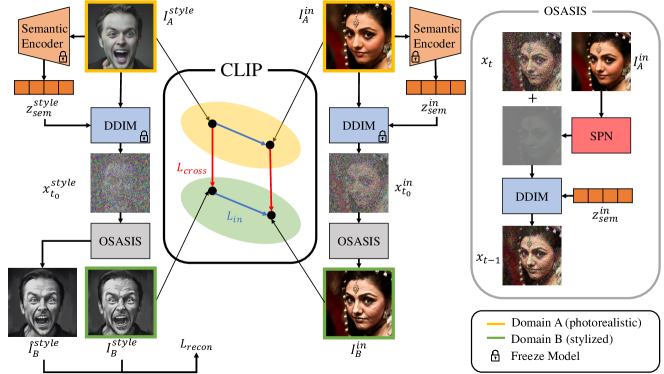
Figure 2: Overview of OSASIS. During finetuning, cross-domain loss compares the photorealistic image (bounded yellow) to its stylized counterparts (bounded green). The in-domain loss compares the style images to the generated counterparts in their respective domains. Reconstruction loss compares the original style image with a reconstructed counterpart. Intuitively, the combination of the directional losses guarantees that for each iteration the generated $I^{\mathrm{in}}_{B}$ is positioned for projection vectors from $I^{\mathrm{style}}_{B}$ and $I^{\mathrm{in}}_{A}$ to be collinear to its cross-domain and in-domain counterparts in the CLIP space.

2.2 Diffusion Autoencoders

DiffAE [23] proposes a semantic encoder $\operatorname{Enc}_{\phi}$ that encodes a given image $\mathbf{x}_{0}$ to a semantically rich latent variable $\mathbf{z}_{\mathrm{sem}}$, represented as:

$$\mathbf{z}_{\mathrm{sem}}=\operatorname{Enc}_{\phi}\left(\mathbf{x}_{0}\right).$$ (6)

This latent variable has been shown to be linear, decodable, and semantically meaningful, hence being an attractive property that our model seeks to leverage. Similar to the aforementioned forward DDIM, DiffAE is also able to encode an image given $\mathbf{z}_{\mathrm{sem}}$ to a fully reconstructable latent $\mathbf{x}_{T}$ by Eq. 7, in which we denote forward DiffAE. Correspondingly, the forward DiffAE encoded latent $\mathbf{x}_{T}$ can be decoded by conditioning itself and $\mathbf{z}_{\mathrm{sem}}$ to the reverse process defined as Eq. 8, referred to as reverse DiffAE.

$$\mathbf{x}_{t+1}=\sqrt{\alpha_{t+1}}f_{\theta}(\mathbf{x}_{t},t,\mathbf{z}_{\mathrm{sem}})+\sqrt{1-\alpha_{t+1}}\epsilon_{\theta}(\mathbf{x}_{t},t,\mathbf{z}_{\mathrm{sem}})$$ (7)

$$\mathbf{x}_{t-1}=\sqrt{\alpha_{t-1}}f_{\theta}(\mathbf{x}_{t},t,\mathbf{z}_{\mathrm{sem}})+\sqrt{1-\alpha_{t-1}}\epsilon_{\theta}(\mathbf{x}_{t},t,\mathbf{z}_{\mathrm{sem}})$$ (8)

$$\quad\text{where}\quad f_{\theta}(\mathbf{x}_{t},t,\mathbf{z}_{\mathrm{sem}})=\frac{\mathbf{x}_{t}-\sqrt{1-\alpha_{t}}\epsilon_{\theta}(\mathbf{x}_{t},t,\mathbf{z}_{\mathrm{sem}})}{\sqrt{\alpha_{t}}}$$

3 Methods

Our approach aims to achieve effective stylization by initially disentangling the structural and semantic information of images. To initially disentangle the semantics from the structure, we employ two distinct latent codes: the structural latent code $\mathbf{x}_{\mathbf{t}_{0}}$ and the semantic latent code $\mathbf{z}_{\mathrm{sem}}$. We finetune a pretrained DDIM $\boldsymbol{\epsilon}^{A}_{\theta}$ conditioned on the semantic latent code $\mathbf{z}_{\mathrm{sem}}$ via CLIP directional losses in order to bridge the domain gap between the input and style images. We define structural information as the overall outline of an image, whereas we further deconstruct the semantics of an image into a combination of content and style. Once finetuned, we control the amount of low-level visual features (e.g. texture and color), referred to as style, and high-level visual features (e.g. object and identity), referred to as content during inference. Proper conditioning of $\mathbf{z}_{\mathrm{sem}}$ to the finetuned DDIM allows us to achieve this control, effectively performing stylization. Furthermore, we directly optimize the semantic latent code $\mathbf{z}_{\mathrm{sem}}$ for text-driven manipulation. By combining the optimized latent with the finetuned DDIM, OSASIS is able to produce stylized images with manipulated attributes. Figure 2 provides an overview of our method.

3.1 Training

To ensure that the changes in the CLIP embedding space occur in the desired direction, we prepare a single image $I^{\mathrm{style}}_{B}$ from a stylized domain (denoted domain B) and aim to convert it to a photorealistic domain (denoted domain A). Recent studies have shown that pretrained DMs can generate domain-specific images based on unseen domain images [14, 20]. Building on this, we utilize a pretrained DDPM $\epsilon_{\theta}$ to generate a single image $I^{\mathrm{style}}_{A}$ from domain A that is semantically aligned with $I^{\mathrm{style}}_{B}$. $I^{\mathrm{style}}_{B}$ is encoded to a specific timestep $\mathbf{t}_{0}$ by utilizing the forward DDPM:

$$\mathbf{x}_{\mathbf{t}_{0}}=\sqrt{\alpha_{\mathbf{t}_{0}}}\mathbf{x}_{0}+\sqrt{1-\alpha_{\mathbf{t}_{0}}}\mathbf{z},\quad\mathbf{z}\sim\mathcal{N}(\mathbf{0},\mathbf{I}),$$ (9)

and subsequently from $\mathbf{x}_{\mathbf{t}_{0}}$, $I^{\mathrm{style}}_{A}$ is generated by following the reverse DDPM:

$$\mathbf{x}_{t-1}=\frac{1}{\sqrt{1-\beta_{t}}}(\mathbf{x}_{t}-\frac{\beta_{t}}{\sqrt{1-\alpha_{t}}}\epsilon_{\theta}(\mathbf{x}_{t},t))+\sigma_{t}\mathbf{z},$$ (10)

where $\mathbf{z}\sim\mathcal{N}(\mathbf{0},\mathbf{I})$. After initializing $I^{\mathrm{style}}_{A}$ and $I^{\mathrm{style}}_{B}$, we proceed to freeze a pretrained DDIM $\boldsymbol{\epsilon}^{A}_{\theta}$ and the semantic encoder $\operatorname{Enc}_{\phi}$ proposed by DiffAE, which is utilized during the image encoding process. Additionally, we create a copy of $\boldsymbol{\epsilon}^{A}_{\theta}$ called $\boldsymbol{\epsilon}^{B}_{\theta}$, which is finetuned through a combination of CLIP directional losses and a reconstruction loss. During training, we note that $I^{\mathrm{in}}_{A}$ is generated from the pretrained DiffAE.

Structural Latent Code

$\boldsymbol{\epsilon}^{B}_{\theta}$ optimizes towards generating $I^{\mathrm{in}}_{B}$ that reflects the semantics of the style image. However, since $I^{\mathrm{style}}_{A}$ and $I^{\mathrm{style}}_{B}$ stays fixed while $I^{\mathrm{in}}_{A}$ is constantly generated, it is crucial to carefully choose an encoding process that generates $I^{\mathrm{in}}_{B}$ that preserves the structural integrity of $I^{\mathrm{in}}_{A}$. In order to achieve this, we utilize forward DiffAE to encode $I^{\mathrm{in}}_{A}$ by computing Eq. 7. First, $I^{\mathrm{in}}_{A}$ is encoded into a semantic latent code $\mathbf{z}_{\mathrm{sem}}^{\mathrm{in}}$ = $\operatorname{Enc}_{\phi}$($I^{\mathrm{in}}_{A}$). By following the forward process, $\mathbf{z}_{\mathrm{sem}}^{\mathrm{in}}$ is conditioned to the frozen DDIM $\boldsymbol{\epsilon}^{A}_{\theta}$,

$$\mathbf{x}_{t+1}=\sqrt{\alpha_{t+1}}f_{\theta}(\mathbf{x}_{t},t,\mathbf{z}_{\mathrm{sem}}^{\mathrm{in}})+\sqrt{1-\alpha_{t+1}}\epsilon^{A}_{\theta}(\mathbf{x}_{t},t,\mathbf{z}_{\mathrm{sem}}^{\mathrm{in}})$$ (11)

resulting in $I^{\mathrm{in}}_{A}$ encoded to a structural latent code $\mathbf{x}_{\mathbf{t}_{0}}^{\mathrm{in}}$. The input image is encoded to a specific timestep $\mathbf{t}_{0}$  which can be adjusted to control the level of structure preservation.

Structure-Preserving Network

Although the structural latent code $\mathbf{x}_{\mathbf{t}_{0}}^{\mathrm{in}}$ succeeds in preserving the overall structure of the generated images $I^{\mathrm{in}}_{A}$, the encoding process defined in Eq. 11 inherently adds stochastic noise, which inevitably results in the loss of structural information. To address this, we introduce a structure-preserving network (SPN), which utilizes a 1x1 convolution that effectively preserves the spatial information and structural integrity of $I^{\mathrm{in}}_{A}$. To generate the output of the next timestep $\mathbf{x}_{t-1}$, we use reverse DiffAE with SPN:

$$\mathbf{x}_{t}^{SPN}=SPN(I^{\mathrm{in}}_{A})$$ (12)

$$\mathbf{x}^{\prime}_{t}=\mathbf{x}_{t}+\lambda_{SPN}*\mathbf{x}_{t}^{SPN}$$ (13)

$$\mathbf{x}_{t-1}=\sqrt{\alpha_{t-1}}f_{\theta}(\mathbf{x}^{\prime}_{t},t,\mathbf{z}_{\mathrm{sem}}^{\mathrm{in}})+\sqrt{1-\alpha_{t-1}}\epsilon^{B}_{\theta}(\mathbf{x}_{t}^{\prime},t,\mathbf{z}_{\mathrm{sem}}^{\mathrm{in}})$$ (14)

We add the output of the SPN to $\mathbf{x}_{t}$, e.g. the previous timestep output of $\boldsymbol{\epsilon}^{B}_{\theta}$, and feed it into our training target $\boldsymbol{\epsilon}^{B}_{\theta}$. We regulate the degree of spatial information reflected in the model by multiplying the output of the SPN $\mathbf{x}_{t}^{SPN}$ by $\lambda_{SPN}$. After fully reversing the timesteps, $I^{\mathrm{in}}_{B}$ is generated.

Loss Function

Inspired by MTG [41], we train $\boldsymbol{\epsilon}^{B}_{\theta}$ by optimizing our total loss, which is comprised of the cross-domain loss, in-domain loss, and reconstruction loss. The cross-domain loss aims to align the direction of changes from domain A to domain B, ensuring that the change from $I^{\mathrm{in}}_{A}$ to $I^{\mathrm{in}}_{B}$ is kept consistent with the change from $I^{\mathrm{style}}_{A}$ to $I^{\mathrm{style}}_{B}$. Although the cross-domain loss provides the changes in semantic information for the model to optimize upon, it often leads to unintended changes when implemented alone. Hence the in-domain loss is introduced to provide additional information, measuring the similarity of changes within both domains A and B.

The reconstruction loss provides additional guidance in capturing the cross-domain change from $I^{\mathrm{style}}_{A}$ to $I^{\mathrm{style}}_{B}$. Similar to our encoding process of Eq. 11, $I^{\mathrm{style}}_{A}$ is encoded to a structural latent code $\mathbf{x}_{\mathbf{t}_{0}}^{\mathrm{style}}$ conditioned on semantic latent code $\mathbf{z}_{\mathrm{sem}}^{\mathrm{style}}$. Following Eq. 12- 14, i.e. the process of generating the output of the next timestep conditioned on $\mathbf{z}_{\mathrm{sem}}^{\mathrm{style}}$, $\hat{I}^{\mathrm{style}}_{B}$ is generated. The reconstruction loss is calculated by comparing $\hat{I}^{\mathrm{style}}_{B}$ with $I^{\mathrm{style}}_{B}$, comprised of the $L_{1}$ loss, perceptual similarity loss [37], and the $L_{1}$ CLIP embedding loss. Detailed information regarding the loss function and experimental setup is available in the supplementary material.

3.2 Sampling

Mixing Content and Style

Once trained, the model $\boldsymbol{\epsilon}^{B}_{\theta}$ is capable of stylizing images from domain A to B. Stylizing an image involves mixing two images in its latent space. While this process is straightforward with StyleGAN [11], it is still an ongoing research area for diffusion models. Unlike the original DiffAE which conditions a single semantic latent code $\mathbf{z}_{\mathrm{sem}}$ to the feature maps of DDIM, we discover that properly conditioning $\mathbf{z}_{\mathrm{sem}}$ to the feature maps of $\boldsymbol{\epsilon}^{B}_{\theta}$ achieves content and style mixing. This is done by conditioning $\mathbf{z}_{\mathrm{sem}}^{\mathrm{style}}$ to its low-level feature maps to transfer the style of a style image, and conditioning $\mathbf{z}_{\mathrm{sem}}^{\mathrm{in}}$ to its high-level feature maps to transfer the content of an input image. The change point of conditioning is set as $f_{ch}$. Since $\boldsymbol{\epsilon}^{B}_{\theta}$ is a UNet-based model, conditioning the two latents is symmetrical. To preserve the structural information of the input image, we use $\mathbf{x}_{\mathbf{t}_{0}}^{\mathrm{in}}$ as the structural latent code.

Text-driven Manipulation

Instead of optimizing a model, we directly optimize the semantic latent code of input image $\mathbf{z}_{\mathrm{sem}}^{\mathrm{in}}$ to achieve text-driven manipulation. Similar to previous works [14], we use CLIP directional loss for optimization. After optimization, the optimized $\mathbf{z}_{\mathrm{sem}}^{\mathrm{in}}$ can be passed into the $\boldsymbol{\epsilon}^{B}_{\theta}$to incorporate the style into the image. Comprehensive details about the experimental approach for text-driven manipulation are available in the supplementary material.

4 Experiments

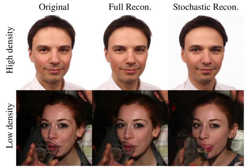
Figure 3: High and Low-density images. Full Recon. refers to reconstruction via conditioning its encoded $\mathbf{z}_{\mathrm{sem}}$ and $\mathbf{x}_{T}$, whereas Stochastic Recon. refers to reconstruction via conditioning its encoded $\mathbf{z}_{\mathrm{sem}}$ and $\mathbf{x}_{T}$ $\sim\mathcal{N}(\mathbf{0},\mathbf{I})$.

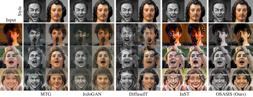
Figure 4: Comparison with other stylization methods. Note that our method successfully preserves the low-density attributes while other baseline methods fail to do so.

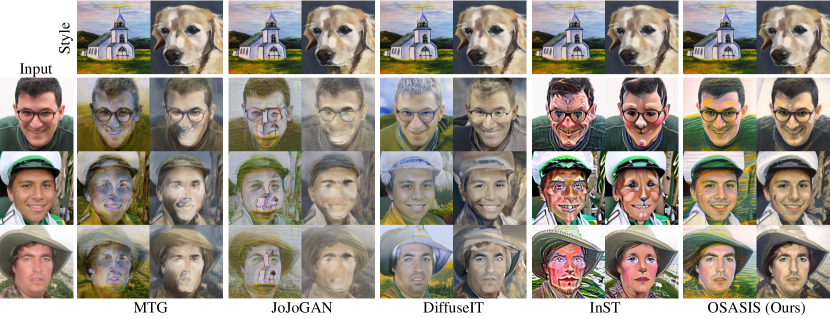
Figure 5: Stylization with OOD reference images. Due to the limited capabilities of GAN-based inversion methods, the baseline methods fail in disentangling the structure and semantics of the style image. This results in structural artifacts being transferred into the output image, whereas OSASIS successfully extracts only the semantics.

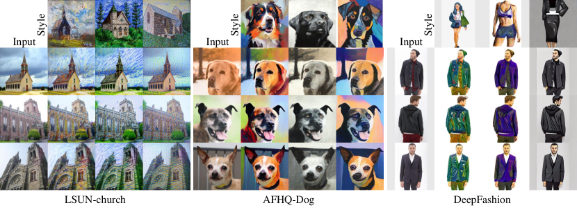
Figure 6: Stylization result of OSASIS on LSUN-church, AFHQ-dog, and DeepFashion.

For evaluating our approach, we focus on images from low-density regions that include rarely encountered attributes during training. This is ideal for demonstrating the structure-preserving ability of our method as low-density region images contain diverse objects and occlusions that obscure the subject. To select these images, we leverage the property that the encoded stochastic subcode $\mathbf{x}_{T}$ tends to show residuals of the original input image rather than being normally distributed, as shown by DiffAE [23]. We randomly select 20,000 images from the FFHQ dataset [11], which is the dataset $\boldsymbol{\epsilon}^{A}_{\theta}$ was trained on. We reconstruct each image using its semantic subcode $\mathbf{z}_{\mathrm{sem}}$ and stochastic subcode $\mathbf{x}_{T}\sim\ \mathcal{N}(\mathbf{0},\mathbf{I})$ (i.e. stochastic reconstruction). We compare the reconstructed image with the original image using perceptual similarity loss [37] to determine the quality of the reconstruction. We hypothesize that high-density region images, comprised of frequently encountered attributes would be reconstructed well, and low-density region images otherwise. Figure 3 shows that our hypothesis is well supported. Finally, we select the images from the top 100 highest LPIPS score group (i.e. low-density) and lowest LPIPS score group (i.e. high-density).

Methods	ArtFID$\downarrow$
	AAHQ	MetFaces	Prev
MTG+HFGI	36.39	38.02	37.27
JoJoGAN+HFGI	40.41	44.74	41.09
DiffuseIT	44.93	53.35	48.18
InST	38.16	50.33	35.86
OSASIS(Ours)	34.89	43.20	33.20
Methods	ID Similarity$\uparrow$
	AAHQ	MetFaces	Prev
MTG+HFGI	0.3730	0.4656	0.4063
JoJoGAN+HFGI	0.5145	0.5207	0.4743
DiffuseIT	0.6992	0.7158	0.6994
InST	0.2253	0.2188	0.2238
OSASIS(Ours)	0.6825	0.7323	0.7029
Methods	Structure Distance$\downarrow$
	AAHQ	MetFaces	Prev
MTG+HFGI	0.0386	0.0350	0.0360
JoJoGAN+HFGI	0.0411	0.0454	0.0430
DiffuseIT	0.0309	0.0300	0.0310
InST	0.0492	0.0443	0.0488
OSASIS(Ours)	0.0361	0.0295	0.0391

Table 1: Quantitative comparison. ArtFID evaluates the pertinence of stylization, whereas ID similarity and structure distance measure whether the stylized image stays true to its original input.

4.1 Qualitative Comparison

In Figure 4, we present a comparative analysis of the performance of OSASIS against other stylization methods. Our results demonstrate that OSASIS outperforms other methods in terms of preserving the overall structure while stylizing. MTG [41] and JoJoGAN [3] use outdated inversion methods that struggle to preserve the diverse structure of input images. To ensure a fair comparison, we employ HFGI [33] for MTG and JoJoGAN, but OSASIS outperforms in terms of preserving the overall structure. Furthermore, GAN-based methods produce unintended modifications, such as changes in facial expressions. Since DiffuseIT [15] stylizes images without training, they struggle to overcome the domain gap between the input and style images. InST [39] utilizes textual inversion to deduce the style image’s concept, and subsequently conditions its generation procedure on this concept. However, the guidance strategy mentioned in [8] leads to unintended image variations, encompassing facial expressions and distinct identities. Moreover, as noted in InST, there are difficulties in faithfully transferring the color of the style images. More qualitative comparison results is provided in the supplementary material.

4.2 Quantitative Comparison

We conduct a quantitative comparison with other methods. By using ArtFID [34] as a metric for effective stylization and the identity similarity measure with ArcFace [4] to assess content preservation. For measuring structure preservation, we employ the structure distance metric [31]. For our source of style images, we select five style images from each of three datasets: i) AAHQ [18], ii) MetFaces  [12], iii) style images used in baseline methods for a fair comparison. In Table 1, we evaluate OSASIS against MTG [41], JoJoGAN [3], DiffuseIT [15], and InST [39]. For our initial pretrained $\boldsymbol{\epsilon}^{A}_{\theta}$ and all baseline models, we use publicly available pretrained models that were trained on FFHQ. As previously mentioned, HFGI [33] is employed to invert input images for MTG and JoJoGAN. Note that Table 1 presents outcomes only for low-density images, while a comprehensive comparison is presented in the supplementary material. Our results indicate that while MTG occasionally achieves a better ArtFID score than our model, we outperform significantly in terms of identity similarity and structure preservation. Additionally, while DiffuseIT excels at preserving the identity and the structure of the image, it exhibits inferior stylization results compared to GAN-based methods due to a domain gap between the input and style images.

4.3 OOD Reference Image

OSASIS is able to stylize images with out-of-domain (OOD) reference images, a feature that is not commonly seen in GAN-based methods. OSASIS can effectively disentangle semantics from the structure, resulting in only the style factor of the style image being transferred to the input image. In contrast, GAN-based methods have entangled style codes in terms of structure and semantics, which makes it difficult to transfer only the style factor from the reference image. As shown in Figure 5, OSASIS is able to stylize images with OOD reference images while preserving its content, whereas other baseline methods suffer from severe artifacts. Although DiffuseIT and InST manage to avoid severe artifacts, they still struggle with addressing domain gap and handling strong concept conditioning.

4.4 Stylization Results on Other Datasets

To evaluate the generalization capabilities of our method across various datasets, we executed stylization on several distinct datasets: AFHQ-dog [2], LSUN-church [36], and DeepFashion [19]. Figure 6 displays the efficacy and versatility of our approach across these diverse datasets. Notably, our method exhibits proficiency beyond facial stylization, adeptly adapting to various image domains.

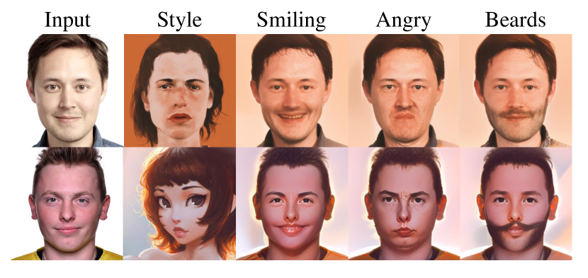
Figure 7: Stylization with text-driven manipulation. The optimized semantic code doesn’t overwrite or harm the structure and style of the image, thus preserving the overall structure while manipulating attributes.

4.5 Stylization with Text-driven Manipulation

For text-driven manipulation, we directly optimize $\mathbf{z}_{\mathrm{sem}}^{\mathrm{in}}$using CLIP directional loss. Similar to DiffusionCLIP [14], we align the $\mathbf{z}_{\mathrm{sem}}^{\mathrm{in}}$ of an input image to a base text prompt (e.g. face) and align a cloned latent with a desired text prompt (e.g. smiling face). Once $\mathbf{z}_{\mathrm{sem}}^{\mathrm{in}}$ is optimized, it can be used to stylize said image with the aforementioned mixing process. In Figure 7, we show our qualitative results of stylization with text-driven manipulation, where our model successfully incorporates the style of a reference image with manipulated attributes, while being robust in content preservation.

4.6 Ablation Study

Latent Code

Furthermore, we conduct ablation studies to shed light on the nature of mixing content and style into the feature maps of the UNet. In the first row of Figure 8, we perform normal stylization on an input image, i.e. by encoding its structural latent code $\mathbf{x}_{\mathbf{t}_{0}}^{\mathrm{in}}$, conditioning $\mathbf{z}_{\mathrm{sem}}^{\mathrm{style}}$ to low-level feature maps, and conditioning $\mathbf{z}_{\mathrm{sem}}^{\mathrm{in}}$ to high-level feature maps. The second row shows the results of the semantic codes being conditioned oppositely. The resulting generated image 1) holds the structural integrity encoded from the structural latent code $\mathbf{x}_{\mathbf{t}_{0}}^{\mathrm{in}}$, 2) preserves the content from the given content image (i.e. identity, facial expressions), and 3) retains the stylized attributes of the given style image (i.e. skin complexion). We show that by conditioning the semantic codes to their respective feature maps, OSASIS achieves control over mixing content and style.

Structure-Preserving Network

Our SPN is implemented to aid the structural latent code $\mathbf{x}_{\mathbf{t}_{0}}^{\mathrm{in}}$ in preserving the overall structure of the stylized image, due to the encoding process Eq.11 being formulated to add stochastic noise. Figure 9 shows the effects of our SPN, where the third column is a stylized sample without, and the fourth column is a stylized sample with SPN. It can be seen that the stochastic latent code $\mathbf{x}_{\mathbf{t}_{0}}^{\mathrm{in}}$ faithfully preserves the overall structure of the image, but without SPN, objects along the edges of content images (e.g. hands, poles, fingers) are distorted.

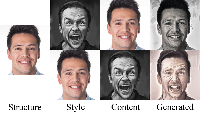
Figure 8: Ablation study of latent codes. The result shows that OSASIS is capable of effectively disentangling the structure from the semantics. By conditioning the semantic codes appropriately, we are able to control the content and style factors in the generated image.

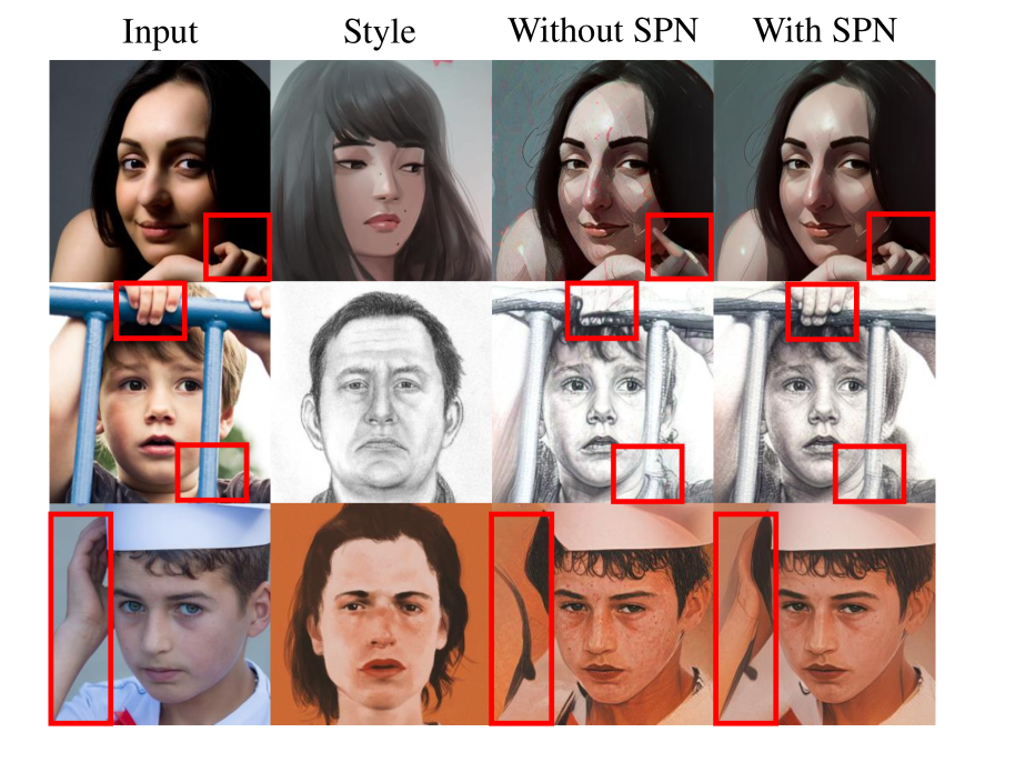
Figure 9: Ablation study of SPN. The results demonstrate that SPN is a crucial to ensure the preservation of the underlying structure while applying the stylization process.

5 Related Work

5.1 One-shot Image Stylization

Stylizing input images with only one reference image originates from neural style transfer, first introduced by Gatys et al. [7]. However, this method requires the stylized image to be optimized every generation, which was addressed by Johnson et al. [10] by introducing an image transform network for fast stylization. However, traditional NST methods are limited in their ability to capture the semantic information of input and style images.

For GAN-based models, One-shot image stylization is achieved by using one-shot adaptation methods, which aims to transfer a generator to a new domain using a single reference image. One-shot adaptation methods typically involve finetuning a generator using only a single reference image. Once the generator is finetuned, these methods can unconditionally generate stylized images, and by using GAN inversion techniques, they also achieve input image stylization. The first successful GAN-based one-shot adaptation method is MTG [41], which uses CLIP directional loss to finetune the generator and mitigate overfitting problems. Other works have since focused on improving generation quality [16], content preservation [38], and entity transfer [40].

In contrast to one-shot adaptation approaches, our method aims to stylize input images with a single reference image, instead of generating stylize synthesized images. Therefore, we refer to our method as one-shot image stylization. From our perspective, the work that is most comparable to our own is JoJoGAN [3]. JoJoGAN generates a training dataset by random style mixing and finetunes a generator to create a style mapper.

5.2 Image Manipulation with Diffusion Models

Image manipulation has advanced significantly in recent years, with methods presented by StyleGAN2 [13] being widely explored. However, the potential of diffusion models for high-quality image manipulation has been elucidated in recent research. DiffAE [23] introduces a semantic encoder that generates semantically meaningful latent vectors for diffusion models, which can be manipulated for attribute editing. DiffusionCLIP [14] demonstrates the effectiveness of diffusion-based text-guided image manipulation by fine-tuning a DDIM with CLIP directional loss. Asyrp [17] uncovers a semantic latent space in the architecture of diffusion models. The authors train the h-space manipulation module with CLIP directional loss, achieving consistent image editing results. While DiffusionCLIP and Asyrp employ CLIP directional loss, their focus is on text-guided manipulation whereas our work targets image-guided manipulation. DiffuseIT [15] aims to perform image translation guided by either text or image using a CLIP and a pretrained ViT  [6]. Their approach leverages the reverse process of DDPM and incorporates CLIP and ViT to guide the image generation process. InST [39] employs textual inversion to extract the concept from a style image. By conditioning the generation process on this extracted concept, InST is able to stylize input images

6 Conclusion

We have introduced OSASIS, a novel one-shot image stylization method based on diffusion models. In contrast to GAN-based and other diffusion-based stylization methods, OSASIS shows robust structure awareness in stylization, effectively disentangling the structure and semantics from an image. While OSASIS demonstrates significant advancements in structure-aware stylization, several limitations exist. A notable constraint of OSASIS is its training time, which is longer than comparison methods. This extended training duration is a trade-off for the method’s enhanced ability to maintain structural integrity and adapt to various styles. Additionally, OSASIS requires training for each style image. This requirement can be seen as a limitation in scenarios where rapid deployment across multiple styles is needed. Despite these challenges, the robustness of OSASIS in preserving the structural integrity of the input images, its effectiveness in out-of-domain reference stylization, and its adaptability in text-driven manipulation make it a promising approach in the field of stylized image synthesis. Future work will address these limitations, particularly in optimizing training efficiency and reducing the necessity for individual style image training, to enhance the practicality and applicability of OSASIS in diverse real-world scenarios.

One-Shot Structure-Aware Stylized Image Synthesis
– Supplementary Material –

Appendix A Training Details

A.1 Training Preparation

In order to train one-shot structure-aware stylized image synthesis (OSASIS), it is necessary to create a photorealistic image, denoted as $I^{\mathrm{style}}_{A}$, that is semantically aligned with a given style image, $I^{\mathrm{style}}_{B}$. This is achieved by first encoding $I^{\mathrm{style}}_{B}$ into a latent code, represented as $\mathbf{x}_{\mathbf{t}_{0}}$ using Eq.9. Then $I^{\mathrm{style}}_{A}$ is generated from $\mathbf{x}_{\mathbf{t}_{0}}$ using Eq.10, utilizing a pretrained DDPM $\epsilon_{\theta}$ during its encoding and generation phases. However, since these processes are stochastic in nature, the resulting $I^{\mathrm{style}}_{A}$ may not always align perfectly with $I^{\mathrm{style}}_{B}$. To overcome this, we generate 30 images from $I^{\mathrm{style}}_{B}$ and evaluate their alignment with $I^{\mathrm{style}}_{B}$using both the $L_{1}$ loss and perceptual similarity loss [37]. We then select the image that is most similar to $I^{\mathrm{style}}_{B}$ as $I^{\mathrm{style}}_{A}$ as the prime candidate. In cases of out-of-domain (OOD) reference images, we match the domain of the pretrained DDPM with the domain of the style image. (e.g. for church style images, we use a pretrained DDPM trained on LSUN-church).

A.2 Structure-Preserving Network

The structure-preserving network (SPN) incorporates a 1x1 convolution to preserve the overall structure of the input image. During the reverse process, the SPN’s output is integrated with the DDIM output. Given that this integration takes place at every timestep, it is crucial for the network to recognize the timestep to effectively control structure preservation. To facilitate this, each block of the SPN is conditioned on the timestep. The detailed architecture of the SPN is illustrated in Figure 9.

A.3 Loss Function Formulation

Cross-Domain Loss

The objective of the cross-domain loss is to align the directional shifts from domain A to domain B, ensuring that the change from $I^{\mathrm{in}}_{A}$ to $I^{\mathrm{in}}_{B}$ is kept consistent with the change from $I^{\mathrm{style}}_{A}$ to $I^{\mathrm{style}}_{B}$. Leveraging the CLIP image encoder $E_{I}$, latent vectors of both the input and style images are extracted. Subtracting these semantically aligned latent vectors results in semantically meaningful directions. The changes in the style and input images are calculated using Eq.15 and Eq.16, respectively. The cosine similarity, as described in Eq. 17, is then used to evaluate the similarity of the two directions.

$$\mathbf{v}_{\mathrm{style}}=E_{I}(I^{\mathrm{style}}_{B})-E_{I}(I^{\mathrm{style}}_{A})$$ (15)

$$\mathbf{v}_{\mathrm{in}}=E_{I}(I^{\mathrm{in}}_{B})-E_{I}(I^{\mathrm{in}}_{A})$$ (16)

$$L_{cross}=1-sim(\mathbf{v}_{style},\mathbf{v}_{in})$$ (17)

In-Domain Loss

The purpose of the in-domain loss is to mitigate unintended changes in the direction of stylization, which can often result in excessive reflection of the style image. This is achieved by measuring the similarity of changes within both domains A and B. Like the cross-domain loss, the in-domain changes are calculated using Eq.18 and Eq.19. The similarity between the two directions is then determined using Eq. 20.

$$\mathbf{v}_{A}=E_{I}(I^{\mathrm{cont}}_{A})-E_{I}(I^{\mathrm{style}}_{A})$$ (18)

$$\mathbf{v}_{B}=E_{I}(I^{\mathrm{cont}}_{B})-E_{I}(I^{\mathrm{style}}_{B})$$ (19)

$$L_{In}=1-sim(\mathbf{v}_{A},\mathbf{v}_{B})$$ (20)

Reconstruction Loss

The reconstruction loss aims to guarantee that the photorealistic style image $I^{\mathrm{style}}_{A}$ can be accurately translated from domain A to domain B. This is achieved by encoding $I^{\mathrm{style}}_{A}$ using $\boldsymbol{\epsilon}^{A}_{\theta}$, which results in the latent vectors $\mathbf{z}_{\mathrm{sem}}^{\mathrm{style}}$ and $\mathbf{x}_{\mathbf{t}_{0}}^{\mathrm{style}}$. The latent vectors are then fed into $\boldsymbol{\epsilon}^{B}_{\theta}$, which generates the predicted domain B style image $\hat{I}^{\mathrm{style}}_{B}$. The reconstruction loss is calculated by comparing $\hat{I}^{\mathrm{style}}_{B}$ with $I^{\mathrm{style}}_{B}$ and the summation of the $L_{1}$ loss, perceptual similarity loss [37], and the $L_{1}$ CLIP embedding loss described in Eq. 22-24. The total reconstruct loss can be computed using Eq. 25.

$$\hat{I^{\mathrm{style}}_{B}}=\epsilon_{\theta}^{B}(\mathbf{z}_{\mathrm{sem}}^{\mathrm{style}},\mathbf{x}_{T}^{\mathrm{style}})$$ (21)

$$L_{re-image}=L_{1}(I^{\mathrm{style}}_{B},\hat{I^{\mathrm{style}}_{B}})$$ (22)

$$L_{re-lpips}=L_{\mathrm{lpips}}(I^{\mathrm{style}}_{B},\hat{I^{\mathrm{style}}_{B}})$$ (23)

$$L_{re-clip}=L_{1}(E_{I}(I^{\mathrm{style}}_{B}),E_{I}(\hat{I^{\mathrm{style}}_{B}}))$$ (24)

$$L_{recon}=\lambda_{re-image}L_{re-image}+\lambda_{re-lpips}L_{re-lpips}$$

$$+\lambda_{re-clip}L_{re-clip}$$ (25)

Total Loss

The total loss is a weighted sum of the aforementioned cross-domain, in-domain, and reconstruction loss, formulated by the following equation:

$$L_{total}=\lambda_{cross}L_{cross}+\lambda_{in}L_{in}+L_{recon}$$ (26)

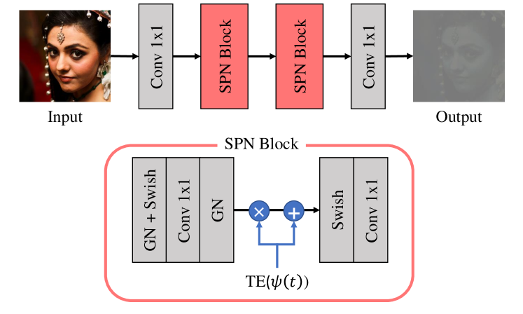
Figure 9: The SPN architecture is comprised of SPN blocks, each consisting of two 1x1 convolutions with group normalizations [35] and swish activations [24]. To incorporate the temporal information of each timestep, the SPN block employs sinusoidal position embeddings [32], represented as $\psi$ for each time step. Timestep embedding (TE) layers are also incorporated, consisting of two linear layers. To condition the SPN block on the current timestep, we use the timestep embedding as a scale and shift parameter of group normalization, which is similar to previous works [5].

Appendix B Sampling Details

B.1 Mixing Content and Style

After training the DDIM $\boldsymbol{\epsilon}^{B}_{\theta}$, we can combine the content of the input images with the style of style images. We achieve this by encoding these images into semantic latent codes, specifically $\mathbf{z}_{\mathrm{sem}}^{\mathrm{in}}$ for input and $\mathbf{z}_{\mathrm{sem}}^{\mathrm{style}}$for style. It is important to note that during training, $\mathbf{z}_{\mathrm{sem}}^{\mathrm{style}}$ comes from $I^{\mathrm{style}}_{A}$, but for sampling, it is sourced from $I^{\mathrm{style}}_{B}$. Using the pretrained DDIM $\boldsymbol{\epsilon}^{A}_{\theta}$, we encode $I^{\mathrm{in}}_{A}$ into a structural latent code $\mathbf{x}_{\mathbf{t}_{0}}^{\mathrm{in}}$. From $\mathbf{x}_{\mathbf{t}_{0}}^{\mathrm{in}}$, $\boldsymbol{\epsilon}^{B}_{\theta}$ generates a stylized image. The process of generating a stylized image is similar to the process of generating $I^{\mathrm{in}}_{B}$ from $I^{\mathrm{in}}_{A}$, as described in Eq.12-14. However, the sampling step involves two semantic latent codes, $\mathbf{z}_{\mathrm{sem}}^{\mathrm{in}}$ and $\mathbf{z}_{\mathrm{sem}}^{\mathrm{style}}$, so the generation process is adjusted accordingly:

$$\mathbf{x}_{t-1}=\sqrt{\alpha_{t-1}}f_{\theta}(\mathbf{x}^{\prime}_{t},t,\mathbf{z}_{\mathrm{sem}}^{\mathrm{in}},\mathbf{z}_{\mathrm{sem}}^{\mathrm{style}})+$$

$$\sqrt{1-\alpha_{t-1}}\epsilon^{B}_{\theta}(\mathbf{x}_{t}^{\prime},t,\mathbf{z}_{\mathrm{sem}}^{\mathrm{in}},\mathbf{z}_{\mathrm{sem}}^{\mathrm{style}})$$ (27)

$\mathbf{z}_{\mathrm{sem}}^{\mathrm{style}}$ is conditioned on low-level feature maps, while $\mathbf{z}_{\mathrm{sem}}^{\mathrm{in}}$ is conditioned on high-level feature maps. The separation between these feature maps is done using $f_{ch}$. The overall sampling process is illustrated in Figure 11.

B.2 Text-driven Manipulation

To enable text-driven image manipulation, we utilize CLIP directional loss, as in previous works [14]. The CLIP directional loss aligns the source-to-target text change with the source-to-target image change, similar to the cross-domain loss. The CLIP text encoder is denoted as $E_{T}$, and the target and source text is represented as $T_{\mathrm{trg}}$ and $T_{\mathrm{src}}$, respectively. The source image $I^{\mathrm{in}}_{A}$ is encoded into semantic and structural latent codes, $\mathbf{z}_{\mathrm{sem}}^{\mathrm{in}}$ and $\mathbf{x}_{\mathbf{t}_{0}}^{\mathrm{in}}$, using DDIM $\boldsymbol{\epsilon}^{A}_{\theta}$. We freeze $\mathbf{x}_{\mathbf{t}_{0}}^{\mathrm{in}}$ and $\boldsymbol{\epsilon}^{A}_{\theta}$, and optimize $\mathbf{z}_{\mathrm{sem}}^{\mathrm{in}}$ to obtain the optimal semantic latent code $\mathbf{z}_{\mathrm{sem}}^{\mathrm{in}*}$. Following this, employing $\mathbf{x}_{\mathbf{t}_{0}}^{\mathrm{in}}$ and $\mathbf{z}_{\mathrm{sem}}^{\mathrm{in}*}$ allows us to derive $I^{\mathrm{in}}_{opt}$ utilizing DDIM $\boldsymbol{\epsilon}^{B}_{\theta}$. The CLIP directional loss is computed as follows:

$$\mathbf{v}_{\mathrm{text}}=E_{T}(T_{\mathrm{trg}})-E_{T}(T_{\mathrm{src}})$$ (28)

$$\mathbf{v}_{\mathrm{image}}=E_{I}(I^{\mathrm{in}}_{opt})-E_{I}(I^{\mathrm{in}}_{A})$$ (29)

$$L_{text}=1-sim(\mathbf{v}_{text},\mathbf{v}_{image})$$ (30)

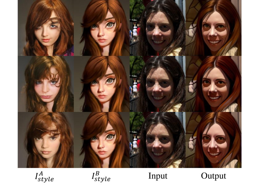
Figure 10: Reliance on $I^{\mathrm{style}}_{A}$. The representation of $I^{\mathrm{style}}_{A}$is stochastic, it can be adjusted through the sampling process transitioning from $I^{\mathrm{style}}_{B}$to $I^{\mathrm{style}}_{A}$. Notably, stylization results maintain consistent visual quality irrespective of variations in $I^{\mathrm{style}}_{A}$.

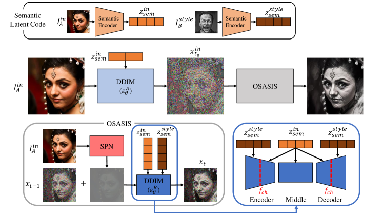
Figure 11: Sampling process of OSASIS. In contrast to the training phase, during the sampling process, $\mathbf{z}_{\mathrm{sem}}^{\mathrm{style}}$ is derived from $I^{\mathrm{style}}_{B}$. To integrate the content from the input with the style of the style image, we condition the DDIM $\boldsymbol{\epsilon}^{B}_{\theta}$, on $\mathbf{z}_{\mathrm{sem}}^{\mathrm{style}}$ and $\mathbf{z}_{\mathrm{sem}}^{\mathrm{in}}$, respectively. This conditioning is separated by $f_{ch}$.

Appendix C Additional Experiments

C.1 Experiments Settings

The encoding timestep $t_{0}$ is set to 500, equating to half of the total timesteps. Based on empirical findings, we define the loss function parameters as $\lambda_{re-image}=10$, $\lambda_{re-lpips}=10$, $\lambda_{re-clip}=30$, $\lambda_{cross}=1$, and $\lambda_{in}=0.5$. For the SPN, we assign $\lambda_{SPN}=0.1$. During sampling, $f_{ch}$ is configured to 32, indicating that $\mathbf{z}_{\mathrm{sem}}^{\mathrm{style}}$conditions up to the 32-resolution feature maps while other blocks are conditioned on $\mathbf{z}_{\mathrm{sem}}^{\mathrm{in}}$.

C.2 Reliance on $I_{A}^{style}$

The generation of $I^{\mathrm{style}}_{A}$ is inherently stochastic, leading to variations in its visual quality. However, the efficacy of our method is not intrinsically tied to the visual fidelity of $I^{\mathrm{style}}_{A}$. As depicted in Figure 10, despite the varying visual presentations of $I^{\mathrm{style}}_{A}$, our method consistently produces reliable stylization results. The resilience of our approach stems from the stylization trajectory determined in the CLIP space, thereby decoupling it from the aesthetic variations of $I^{\mathrm{style}}_{A}$. To mitigate any misalignment that might arise between $I^{\mathrm{style}}_{A}$and $I^{\mathrm{style}}_{B}$, we adopt a systematic sampling methodology, subsequently auto-selecting the most congruent image, as outlined in Training Preparation.

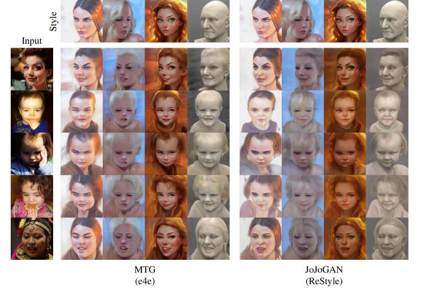
Figure 12: Stylization results of MTG and JoJoGAN.

C.3 Additional Results

In this section, we present additional stylization results and its comparisons with other stylization methods. Figure 12 shows the stylization outcomes of the original MTG [41] and JoJoGAN [3], which utilizes e4e [30] and ReStyle [1] respectively for inversion. Compared to HFGI [33], these methods struggle to preserve the structure of the input image leading to a loss of key elements, such as hands and accessories. Additional stylization results on comparison methods are shown in Figure 13, where OSASIS outperforms other methods in structural preservation while stylizing. Figure 14 shows the stylization results of OOD reference images. Table 2 encapsulates a comprehensive quantitative comparison, encompassing both low and high-density image results.

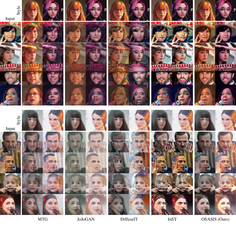
Figure 13: Stylization result of OSASIS and comparison methods.

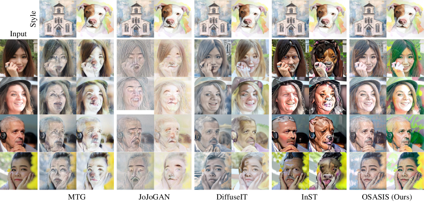
Figure 14: Stylization result of OSASIS and comparison methods with OOD reference images.

	Methods	ArtFID$\downarrow$			ID Similarity$\uparrow$			Structure Similarity$\downarrow$
		AAHQ	MetFaces	Prev	AAHQ	MetFaces	Prev	AAHQ	MetFaces	Prev
High Density	MTG	34.54	34.73	35.18	0.2026	0.2562	0.2219	0.0403	0.0493	0.0477
	MTG+HFGI	35.03	37.19	36.23	0.3260	0.4362	0.3688	0.0357	0.0375	0.0370
	JoJoGAN	41.93	43.99	36.95	0.3783	0.3477	0.3280	0.0389	0.0465	0.0441
	JoJoGAN+HFGI	41.20	43.32	39.29	0.4927	0.4921	0.4353	0.0327	0.0385	0.0346
	DiffuseIT	44.03	52.92	46.56	0.6922	0.7259	0.6970	0.0254	0.0252	0.0250
	InST	31.84	46.13	30.69	0.1760	0.1864	0.1815	0.0390	0.0326	0.0383
	OSASIS(Ours)	33.06	41.66	30.46	0.7191	0.7520	0.7303	0.0367	0.0350	0.0345
Low Density	MTG	36.19	36.52	35.93	0.2228	0.2516	0.2263	0.0608	0.0557	0.0574
	MTG+HFGI	36.39	38.02	37.27	0.3730	0.4656	0.4063	0.0386	0.0350	0.0360
	JoJoGAN	43.51	45.23	38.49	0.3763	0.3579	0.3319	0.0589	0.00631	0.0605
	JoJoGAN+HFGI	40.41	44.74	41.09	0.5145	0.5207	0.4743	0.0411	0.0454	0.0403
	DiffuseIT	44.93	53.35	48.18	0.6992	0.7158	0.6994	0.0309	0.0300	0.0310
	InST	38.16	50.33	35.86	0.2253	0.2188	0.2238	0.0492	0.0443	0.0488
	OSASIS(Ours)	34.89	43.20	33.20	0.6825	0.7323	0.7029	0.0361	0.0295	0.0391

Table 2: Quantitative comparison.

References

- Alaluf et al. [2021] Yuval Alaluf, Or Patashnik, and Daniel Cohen-Or. Restyle: A residual-based stylegan encoder via iterative refinement. In Proceedings of the IEEE/CVF International Conference on Computer Vision, pages 6711–6720, 2021.
- Choi et al. [2020] Yunjey Choi, Youngjung Uh, Jaejun Yoo, and Jung-Woo Ha. Stargan v2: Diverse image synthesis for multiple domains. In Proceedings of the IEEE/CVF conference on computer vision and pattern recognition, pages 8188–8197, 2020.
- Chong and Forsyth [2022] Min Jin Chong and David Forsyth. Jojogan: One shot face stylization. In European Conference on Computer Vision, pages 128–152. Springer, 2022.
- Deng et al. [2019] Jiankang Deng, Jia Guo, Niannan Xue, and Stefanos Zafeiriou. Arcface: Additive angular margin loss for deep face recognition. In Proceedings of the IEEE/CVF conference on computer vision and pattern recognition, pages 4690–4699, 2019.
- Dhariwal and Nichol [2021] Prafulla Dhariwal and Alexander Nichol. Diffusion models beat gans on image synthesis. Advances in Neural Information Processing Systems, 34:8780–8794, 2021.
- Dosovitskiy et al. [2020] Alexey Dosovitskiy, Lucas Beyer, Alexander Kolesnikov, Dirk Weissenborn, Xiaohua Zhai, Thomas Unterthiner, Mostafa Dehghani, Matthias Minderer, Georg Heigold, Sylvain Gelly, et al. An image is worth 16x16 words: Transformers for image recognition at scale. arXiv preprint arXiv:2010.11929, 2020.
- Gatys et al. [2016] Leon A Gatys, Alexander S Ecker, and Matthias Bethge. Image style transfer using convolutional neural networks. In Proceedings of the IEEE conference on computer vision and pattern recognition, pages 2414–2423, 2016.
- Ho and Salimans [2021] Jonathan Ho and Tim Salimans. Classifier-free diffusion guidance. In NeurIPS 2021 Workshop on Deep Generative Models and Downstream Applications, 2021.
- Ho et al. [2020] Jonathan Ho, Ajay Jain, and Pieter Abbeel. Denoising diffusion probabilistic models. Advances in Neural Information Processing Systems, 33:6840–6851, 2020.
- Johnson et al. [2016] Justin Johnson, Alexandre Alahi, and Li Fei-Fei. Perceptual losses for real-time style transfer and super-resolution. In Computer Vision–ECCV 2016: 14th European Conference, Amsterdam, The Netherlands, October 11-14, 2016, Proceedings, Part II 14, pages 694–711. Springer, 2016.
- Karras et al. [2019] Tero Karras, Samuli Laine, and Timo Aila. A style-based generator architecture for generative adversarial networks. In Proceedings of the IEEE/CVF conference on computer vision and pattern recognition, pages 4401–4410, 2019.
- Karras et al. [2020a] Tero Karras, Miika Aittala, Janne Hellsten, Samuli Laine, Jaakko Lehtinen, and Timo Aila. Training generative adversarial networks with limited data. Advances in neural information processing systems, 33:12104–12114, 2020a.
- Karras et al. [2020b] Tero Karras, Samuli Laine, Miika Aittala, Janne Hellsten, Jaakko Lehtinen, and Timo Aila. Analyzing and improving the image quality of stylegan. In Proceedings of the IEEE/CVF conference on computer vision and pattern recognition, pages 8110–8119, 2020b.
- Kim et al. [2022] Gwanghyun Kim, Taesung Kwon, and Jong Chul Ye. Diffusionclip: Text-guided diffusion models for robust image manipulation. In Proceedings of the IEEE/CVF Conference on Computer Vision and Pattern Recognition, pages 2426–2435, 2022.
- Kwon and Ye [2022a] Gihyun Kwon and Jong Chul Ye. Diffusion-based image translation using disentangled style and content representation. arXiv preprint arXiv:2209.15264, 2022a.
- Kwon and Ye [2022b] Gihyun Kwon and Jong Chul Ye. One-shot adaptation of gan in just one clip. arXiv preprint arXiv:2203.09301, 2022b.
- Kwon et al. [2022] Mingi Kwon, Jaeseok Jeong, and Youngjung Uh. Diffusion models already have a semantic latent space. arXiv preprint arXiv:2210.10960, 2022.
- Liu et al. [2021] Mingcong Liu, Qiang Li, Zekui Qin, Guoxin Zhang, Pengfei Wan, and Wen Zheng. Blendgan: Implicitly gan blending for arbitrary stylized face generation. Advances in Neural Information Processing Systems, 34:29710–29722, 2021.
- Liu et al. [2016] Ziwei Liu, Ping Luo, Shi Qiu, Xiaogang Wang, and Xiaoou Tang. Deepfashion: Powering robust clothes recognition and retrieval with rich annotations. In Proceedings of IEEE Conference on Computer Vision and Pattern Recognition (CVPR), 2016.
- Meng et al. [2022] Chenlin Meng, Yutong He, Yang Song, Jiaming Song, Jiajun Wu, Jun-Yan Zhu, and Stefano Ermon. SDEdit: Guided image synthesis and editing with stochastic differential equations. In International Conference on Learning Representations, 2022.
- Ojha et al. [2021] Utkarsh Ojha, Yijun Li, Jingwan Lu, Alexei A Efros, Yong Jae Lee, Eli Shechtman, and Richard Zhang. Few-shot image generation via cross-domain correspondence. In Proceedings of the IEEE/CVF Conference on Computer Vision and Pattern Recognition, pages 10743–10752, 2021.
- Pinkney and Adler [2020] Justin NM Pinkney and Doron Adler. Resolution dependent gan interpolation for controllable image synthesis between domains. arXiv preprint arXiv:2010.05334, 2020.
- Preechakul et al. [2022] Konpat Preechakul, Nattanat Chatthee, Suttisak Wizadwongsa, and Supasorn Suwajanakorn. Diffusion autoencoders: Toward a meaningful and decodable representation. In Proceedings of the IEEE/CVF Conference on Computer Vision and Pattern Recognition, pages 10619–10629, 2022.
- Ramachandran et al. [2017] Prajit Ramachandran, Barret Zoph, and Quoc V Le. Searching for activation functions. arXiv preprint arXiv:1710.05941, 2017.
- Rombach et al. [2022] Robin Rombach, Andreas Blattmann, Dominik Lorenz, Patrick Esser, and Björn Ommer. High-resolution image synthesis with latent diffusion models. In Proceedings of the IEEE/CVF Conference on Computer Vision and Pattern Recognition, pages 10684–10695, 2022.
- Saharia et al. [2022a] Chitwan Saharia, William Chan, Saurabh Saxena, Lala Li, Jay Whang, Emily Denton, Seyed Kamyar Seyed Ghasemipour, Burcu Karagol Ayan, S Sara Mahdavi, Rapha Gontijo Lopes, et al. Photorealistic text-to-image diffusion models with deep language understanding. arXiv preprint arXiv:2205.11487, 2022a.
- Saharia et al. [2022b] Chitwan Saharia, Jonathan Ho, William Chan, Tim Salimans, David J Fleet, and Mohammad Norouzi. Image super-resolution via iterative refinement. IEEE Transactions on Pattern Analysis and Machine Intelligence, 2022b.
- Song et al. [2021] Guoxian Song, Linjie Luo, Jing Liu, Wan-Chun Ma, Chunpong Lai, Chuanxia Zheng, and Tat-Jen Cham. Agilegan: stylizing portraits by inversion-consistent transfer learning. ACM Transactions on Graphics (TOG), 40(4):1–13, 2021.
- Song et al. [2020] Jiaming Song, Chenlin Meng, and Stefano Ermon. Denoising diffusion implicit models. In International Conference on Learning Representations, 2020.
- Tov et al. [2021] Omer Tov, Yuval Alaluf, Yotam Nitzan, Or Patashnik, and Daniel Cohen-Or. Designing an encoder for stylegan image manipulation. ACM Transactions on Graphics (TOG), 40(4):1–14, 2021.
- Tumanyan et al. [2022] Narek Tumanyan, Omer Bar-Tal, Shai Bagon, and Tali Dekel. Splicing vit features for semantic appearance transfer. In Proceedings of the IEEE/CVF Conference on Computer Vision and Pattern Recognition, pages 10748–10757, 2022.
- Vaswani et al. [2017] Ashish Vaswani, Noam Shazeer, Niki Parmar, Jakob Uszkoreit, Llion Jones, Aidan N Gomez, Łukasz Kaiser, and Illia Polosukhin. Attention is all you need. Advances in neural information processing systems, 30, 2017.
- Wang et al. [2022] Tengfei Wang, Yong Zhang, Yanbo Fan, Jue Wang, and Qifeng Chen. High-fidelity gan inversion for image attribute editing. In Proceedings of the IEEE/CVF Conference on Computer Vision and Pattern Recognition, 2022.
- Wright and Ommer [2022] Matthias Wright and Björn Ommer. Artfid: Quantitative evaluation of neural style transfer. In Pattern Recognition: 44th DAGM German Conference, DAGM GCPR 2022, Konstanz, Germany, September 27–30, 2022, Proceedings, pages 560–576. Springer, 2022.
- Wu and He [2018] Yuxin Wu and Kaiming He. Group normalization. In Proceedings of the European conference on computer vision (ECCV), pages 3–19, 2018.
- Yu et al. [2015] Fisher Yu, Ari Seff, Yinda Zhang, Shuran Song, Thomas Funkhouser, and Jianxiong Xiao. Lsun: Construction of a large-scale image dataset using deep learning with humans in the loop. arXiv preprint arXiv:1506.03365, 2015.
- Zhang et al. [2018] Richard Zhang, Phillip Isola, Alexei A Efros, Eli Shechtman, and Oliver Wang. The unreasonable effectiveness of deep features as a perceptual metric. In Proceedings of the IEEE conference on computer vision and pattern recognition, pages 586–595, 2018.
- Zhang et al. [2022a] Yabo Zhang, Yuxiang Wei, Zhilong Ji, Jinfeng Bai, Wangmeng Zuo, et al. Towards diverse and faithful one-shot adaption of generative adversarial networks. In Advances in Neural Information Processing Systems, 2022a.
- Zhang et al. [2023] Yuxin Zhang, Nisha Huang, Fan Tang, Haibin Huang, Chongyang Ma, Weiming Dong, and Changsheng Xu. Inversion-based style transfer with diffusion models. In Proceedings of the IEEE/CVF Conference on Computer Vision and Pattern Recognition, pages 10146–10156, 2023.
- Zhang et al. [2022b] Zicheng Zhang, Yinglu Liu, Congying Han, Tiande Guo, Ting Yao, and Tao Mei. Generalized one-shot domain adaption of generative adversarial networks. arXiv preprint arXiv:2209.03665, 2022b.
- Zhu et al. [2021] Peihao Zhu, Rameen Abdal, John Femiani, and Peter Wonka. Mind the gap: Domain gap control for single shot domain adaptation for generative adversarial networks. In International Conference on Learning Representations, 2021.