Real-time tracking of moving objects from scattering matrix in real-world microwave imaging
Seong-Ho Son
son@sch.ac.krDepartment of ICT Convergence, Soonchunhyang University, Asan, 31538, Republic of Korea
Department of Mechanical Engineering, Soonchunhyang University, Asan, 31538, Republic of Korea
Kwang-Jae Lee
reolee0122@etri.re.krRadio Environment & Monitoring Research Group, Electronics and Telecommunications Research Institute, Daejeon, 34129, Republic of Korea
Won-Kwang Park
parkwk@kookmin.ac.krDepartment of Information Security, Cryptology, and Mathematics, Kookmin University, Seoul 02707, Republic of Korea
Abstract
The problem of the real-time microwave imaging of small, moving objects from a scattering matrix, whose elements are measured scattering parameters, without diagonal elements is considered herein. An imaging algorithm based on a Kirchhoff migration operated at single frequency is designed, and its mathematical structure is investigated by establishing a relationship with an infinite series of Bessel functions of integer order and antenna configuration. This is based on the application of the Born approximation to the scattering parameters of small objects. The structure explains the reason for the detection of moving objects via a designed imaging function and supplies its some properties. To demonstrate the strengths and weaknesses of the proposed algorithm, various simulations with real-data are conducted.
The real-time tracking of unknown objects using microwaves is an important and interesting inverse scattering problem that arises in fields such as physics, engineering, and military services, and is nowadays highly related to human life [1, 2, 3, 4, 5, 6, 7]. Most studies have focused on the development of detection algorithms for unknown objects located in a wide area; however, the detection of the movements of small objects or changes in permittivity/conductivity distributions in small or narrow regions has not been sufficiently investigated. Detecting small objects is not an easy problem to solve but can be applied to various real-world problems, such as the diagnoses of cerebral hemorrhages, imaging of crack propagations in walls or bridges, and through-wall imaging. In general, objects exhibit material properties (permittivities and conductivities) that are different from their background media; thus, most studies have focused on retrieving complete information about these properties. Unfortunately, owing to the intrinsic ill-posedness and nonlinearity of the inverse scattering problem, it cannot be successfully and satisfactorily resolved.
To solve this problem, various inversion techniques and corresponding computational environments have been investigated. The most popular and appropriate approaches in real-world applications are based on the Newton-type iteration scheme, which involves retrieving information about the shape, location, and material properties of unknown objects (minimizers); these unknown objects minimize the discrete norm (generally, norm) between the measured data in the presence of true and man-made objects. We refer to several remarkable studies [8, 9, 10, 11, 12, 13, 14].
Although iteration-based techniques have shown their feasibilities, some preceding conditions, such as good initial guesses that are close to the objects, a priori information about unknown objects, appropriate regularization terms significantly dependent on the problem, evaluations of complex Fréchet (or domain) derivatives, must be fulfilled to guarantee successful iteration procedures. Furthermore, large computational costs are still incurred, and extensions to multiple objects still prove to be difficult. Hence, Newton-type iteration schemes are not appropriate in designing real-time detection of moving objects.
As alternatives, various non-iterative algorithms have been investigated, e.g., bifocusing method [15, 16, 17, 18], direct sampling method [19, 20, 21, 22], MUltiple SIgnal Classification (MUSIC) algorithm [23, 24, 25, 26], linear sampling method [27, 28, 29, 30], topological derivatives [31, 32, 33, 34], Kirchhoff and subspace migrations [35, 36, 37, 38], and orthogonality sampling method [39, 40, 41, 42]. It is worth mentioning that although complete information about unknown objects cannot be retrieved via non-iterative algorithms, such algorithms are fast, effective, and stable in detecting multiple objects without any a priori information. So, instead of completely reconstructing the objects, it would be appropriate to design a real-time algorithm for detecting moving objects. Let us emphasize that in order to apply MUSIC or subspace migration for identifying moving objects, a careful threshold of singular values of the scattering matrix is essential. Topological derivative based technique or linear sampling method are very stable and effective non-iterative techniques but additional operations such as solving adjoint problems or nonlinear integral equations are required. Hence, these methods would be inappropriate as real-time detection techniques. Fortunately, bifocusing method, direct and orthogonality sampling methods with multiple sources, and Kirchhoff migration require no additional operations; therefore, we believe that they can be applicable to design a real-time detection algorithm.
Herein, we apply Kirchhoff migration for a real-time tracking of moving small objects from the scattering matrix, whose elements are measured scattering parameters at a fixed frequency. In contrast to the traditional studies in inverse scattering problems, the diagonal elements of a scattering matrix cannot be determined from a microwave machine, i.e., scattering parameters cannot be obtained when the transmitting and receiving antennas are at the same location. Considering such a limitation, an imaging function based on the Kirchhoff migration for tracking moving objects is designed, and its mathematical structure was rigorously analyzed by establishing a relation with an infinite series of Bessel functions of integer order and antenna configurations. Based on this relation, we can demonstrate that designed tracking algorithm is fast and effective. Moreover, it is possible to guarantee unique determination of moving objects. To illustrate the feasibilities of the designed technique and to avoid committing inverse crimes, numerical simulations are performed with experimental data generated by a microwave machine [43].
The remainder of this paper is organized as follows. Section 1 briefly introduces the forward problem and scattering parameters caused by the presence of objects. In Section 2, we describe the Kirchhoff migration-based imaging algorithm without the diagonal elements of the scattering matrix, analyze the mathematical structure of the imaging function by establishing an infinite series of Bessel functions of integer order and antenna setting, and discuss some properties of the imaging function. Section 3 discusses the results of the simulation, which used real-world data to demonstrate the effectiveness of the algorithm. Section 4 concludes the paper.
1 The forward problem and scattering parameters
In this section, the forward model and scattering parameters are briefly introduced in the presence of a set of objects with small diameter. Let , , be an (cross-sectional) object with location at time and denotes the collection of . Throughout this study, all are included in a homogeneous region of interest (ROI) and surrounded by several transmitting and receiving antennas located at , , with . We denote as the collection of antennas and assume that all and are characterized by their dielectric permittivity and electric conductivity at a given angular frequency , i.e., the magnetic permeability of all objects are constant such that , . We denote and as the piecewise constant permittivity and conductivity
respectively. With this, we further assume that the following relationships hold for ,
(1)
where denotes the diameter of .
Let be the time-harmonic incident electric field in a homogeneous medium resulting from a point current density at . Then, based on the Maxwell equation, satisfies
Let be the corresponding total electric field due to the existence of measured at . Then, satisfies
with the transmission condition on , . Here, the time-harmonic dependence is assumed.
The scattering parameter (parameter) , , is defined as the ratio of the output voltage at the and the input voltage at the at the time . Let and be the scattering parameter data in the presence and absence of , respectively, and denote as the scattered field -parameter. Based on the simulation setup introduced in recent works [43, 44, 45], only the -components of and can be handled so that by denoting and as the -component of incident and total fields, respectively, can be presented as the following integral equation formula:
(2)
where denotes the lossless background wavenumber that satisfies , refer to [46].
2 Kirchhoff migration for a real-time detection: introduction, analysis, and some properties
2.1 Introduction to imaging function of the Kirchhoff migration
Herein, we introduce the traditional imaging function of the Kirchhoff migration and apply it for a real-time mornitoring of moving objects generated from the scattering matrix such that
(3)
Unfortunately, it is very difficult to apply (2) directly to design an imaging function because exact expression of is unknown. Since we already assumed the condition (1) holds, every can be regarded as an object with small diameter. Thus, based on [47], it is possible to apply the Born approximation so that (2) can be approximated as
(4)
and correspondingly, applying (4) to (3), can be decomposed as
(5)
Based on the structure of the above decomposition, let us generate the following unit vector: for each ,
Now, let us define an inner product on the Lebesgue space such that
(6)
Then, based on the orthogonal property of the , we can examine that the value of will reach its maximum value when . Correspondingly, the following imaging function of the Kirchhoff migration can be introduced: for each ,
(7)
Based on the (5) and (6), the value of is expected to reach its maximum value when . For a detailed description of the imaging function, we refer to [36].
Contrary to the traditional simulation setup, each antenna is used for signal transmission, whereas the remaining antennas are used for signal reception. Therefore, the value of for , i.e., the diagonal elements of cannot be determined so that generated scattering matrix is of the following form
For a related discussions, we recommend some references [48, 25, 49]. In this study, we set instead of the unknown measurement data and the following scattering matrix is considered for the design of the imaging function:
(8)
We refer to [44, 40, 50] for an explanation of why the diagonal elements of scattering matrix were set to zero. Although, the diagonal elements are missing, the following imaging function can be introduced with a similar way to (7): for each ,
(9)
Theoretical reason of the applicability of real-time object detection is discussed next.
2.2 Structure of the imaging function
In order to explain the availability of real-time detection of moving object, mathematical structure of the designed imaging function is carefully explored by establishing a relationship with an infinite series of Bessel functions.
Theorem 2.1(Structure of imaging function).
Let and . If for all , then can be represented as follows:
(10)
where is a Bessel function of the order of the first kind,
Proof.
Since for all , the following asymptotic form of the Hankel function holds (see [51, Theorem 2.5], for instance)
(11)
Then, since
and
we can derive
where and .
Since and the following Jacobi-Anger expansion formula holds uniformly
Finally, by taking the absolute value, we can obtain the result (10). This completes the proof.
∎
2.3 Various properties of imaging function
On the basis of the result (10), we can explore some properties of imaging function as follows.
Property 2.1(Availability of detection).
Since and for , map of will contain peaks of large magnitudes when . Hence, the locations of the moving objects can be imaged via the map of . Furthermore, owing to the oscillating property of the Bessel functions, some artifacts will be included on the map of .
Property 2.2(Dependence of the material properties).
If then since and , we have
Hence, we can conclude that the value of significantly depends on the size, permittivity, and conductivity of the object. This means that if the size, permittivity, and conductivity of an object is considerably larger than those of the others, peaks of large magnitude will appear on the map of at the location of this object because for and .
Property 2.3(Ideal conditions for a proper detection).
Based on the structure of the factor , it disturbs the detection of objects. Thus, eliminating the factors and will guarantee good results. Notice that if one can increase as much as possible () or apply extremely high frequency (), then their effects can be reduced but this is inappropriate for real-world applications.
Property 2.4(Practical condition for a proper detection).
To reduce the adverse effect of , a condition must be found to satisfy the following equation:
Since we have no a priori information of objects, cannot be eliminated. This means that we must find a condition such that
Based on the periodic property of the cosine and sine functions, the effect of can be reduced when even number of antennas are uniformly distributed on a circular array and total number of antennas is greater than . This means that the array configuration of the antennas affects the imaging quality and this is the theoretical reason for the even number of antennas and their symmetric location with respect to the origin in general. We refer to [52, 34, 44] for a similar phenomenon in various imaging techniques.
Property 2.5(On the imaging of objects close to an antenna).
On the imaging of objects, the distance between each objects or between object and antennas significantly influences the imaging performance because the integral equation formula (2) holds for well-separated objects and Theorem 2.1 holds when . If an object is very close to an antenna at time such that
then based on the asymptotic form of the Hankel function
some elements of will be very large valued so that unexpected imaging results (appearance of several artifacts with large magnitudes, invisible of objects, etc.) will be obtained. Here, denotes the Euler–Mascheroni constant.
Finally, based on the Property 2.1, we can derive following important result of the unique determination.
Corollary 2.1(Unique determination of moving objects).
For given angular frequency , the moving objects at each time can be detected uniquely through the map of with the same condition of Theorem 2.1.
3 Simulation results with experimental data
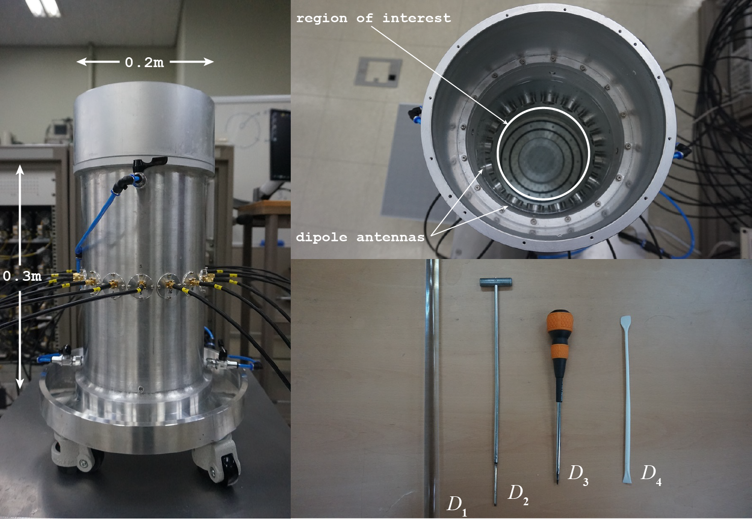
In this section, various numerical simulation results with experimental data are shown for demonstrating the feasibility of the Kirchhoff migration and supporting the theoretical result. For the simulation, dipole antennas equally distributed on a circle with a diameter of are placed into a cylindrical tank with a height of and a diameter of to satisfy the condition in Property 2.4. The tank was filled with water such that at , where denotes the vacuum permittivity. Under the current simulation configuration, since (i.e., ), we set the ROI as a circle centered at the origin with radius of to satisfy the condition for all , refer to the condition of Theorem 2.1 and discussion of Property 2.5. Throughout this paper, the elements of are generated using a microwave machine manufactured by Electronics and Telecommunications Research Institute (ETRI), refer to [43]. For describing objects, the cross-section of four long objects , , are chosen. Table 1 presents the material properties of each object and Figure 1 exhibits the manufactured microwave machine, antenna arrangements, and selected objects.
Object (cross-section)
Permittivity
Conductivity ()
Diameter ()
: plastic bar
(approximately)
(approximately)
: steel barpi
: steel barpi
: plastic bar
(approximately)
(approximately)
Table 1: Values of permittivities, conductivities, and sizes of objects.
Figure 1: Photos of microwave machine and objects , .
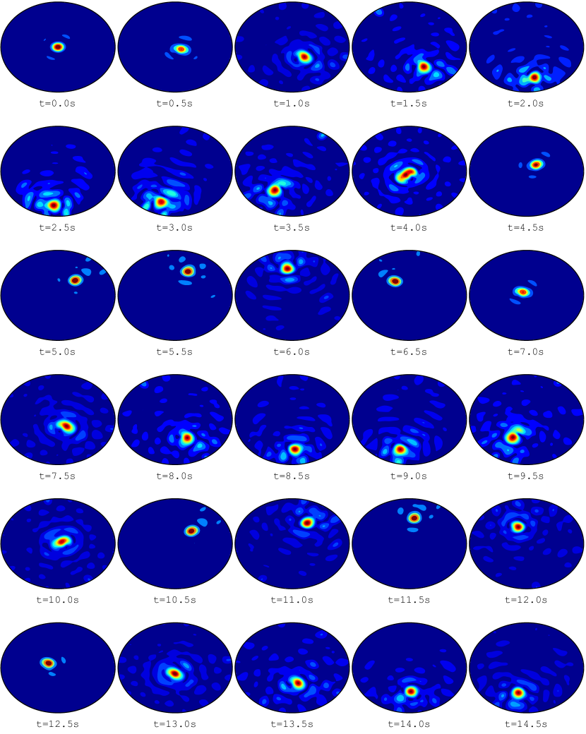
Example 3.1(Tracking of single moving object).
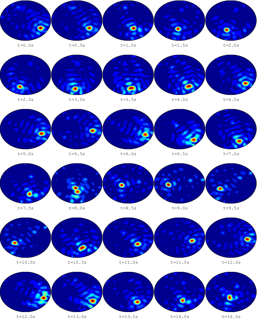
Figure 2 shows the maps of for a single, moving object . Although some artifacts are included on the map, it is possible to track the moving object. Note that at some time (e.g., , , , etc.), the artifacts were eliminated. We cannot explain the exact reason of this phenomenon, but we believe that at that moments, of (10).
Figure 2: (Example 3.1) Maps of for moving object .
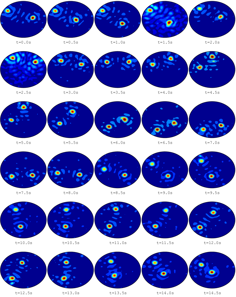
Example 3.2(Tracking of moving objects: same radii and material properties).
Figure 3 shows the maps of for two moving objects and with almost the same radii and material properties, i.e., for and . Similar to the result in Example 3.1, the track of the moving objects can be recognized even though some artifacts degrade the imaging quality. Fortunately, in contrast to Example 3.1, the artifacts do not disturb the recognition of the moving objects but at certain instances and , significantly large amounts of artifacts appear. It is interesting to observe that although the material properties and sizes of two objects are the same, the magnitudes are different at certain instances. For example, by comparing the maps of at and , we can observe that there is no significant change of locations, but the magnitudes changed. Unfortunately, the truth behind this phenomenon cannot be estimated at present, but the distance between the object and antennas may possibly be the reason, refer to Property 2.5.
Figure 3: (Example 3.2) Maps of for moving objects and .
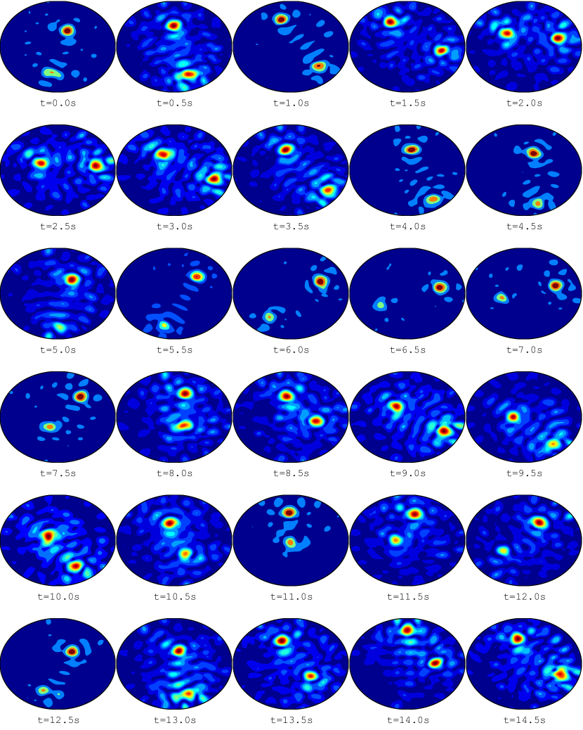
Example 3.3(Tracking of moving objects: different radii and material properties).
Now, we consider the tracking of moving objects and . On the basis of the result in Figure 4, we can observe that a peak of large magnitude appears when because the size of is significantly larger than that of i.e., for and , refer to Property 2.2. Similar to the results in Example 3.2, some artifacts are included on the map of ; however, they were disappeared at certain instances, e.g., , , and .
Figure 4: (Example 3.3) Maps of for moving objects and .
Example 3.4(Tracking of moving objects: same radii but different material properties).
For the final example, we present the simulation result for moving objects and with the same size but different material properties such that for and . Figure 5 shows the maps of , and we can observe that it is impossible to recognize the movement of because the value of at is significantly smaller than that of at . It is interesting to observe that when an object moves quickly, few ghost replicas are exhibited on the map, e.g., two peaks of large magnitude appeared at when moved quickly.
Figure 5: (Example 3.4) Maps of for moving objects and .
4 Conclusion and perspectives
Owing to the existence of small, moving objects and the non-iterative Kirchhoff migration technique in inverse scattering problems, we designed a real-time algorithm for imaging the moving objects on the basis of the representation formula of the scattering parameters. To examine the feasibility and explore some properties of the designed algorithm, we proved that the imaging function could be represented as the total and array configuration of the antennas and an infinite series of Bessel functions of integer order.
Numerical simulations were performed using experimental data generated by the ETRI to demonstrate that the Kirchhoff migration is very effective for a real-time detection of moving objects in microwave imaging. However, the algorithm’s application is currently restricted to the detection of small objects; therefore, further applications to the detection of the movements of arbitrary shaped extended objects or the evolution of crack-like defects must be considered. Forthcoming studies will focus on designing appropriate imaging algorithms, performing related mathematical analyses, and conducting related simulations.
Acknowledgments
This research was supported by the National Research Foundation of Korea (NRF) grant funded by the Korea government (MSIT) (NRF-2020R1A2C1A01005221) and the Soonchunhyang University research fund.
References
Atay et al. [2016]
T. Atay, M. Kaplan,
Y. Kilic, N. Karapinar,
A-Track: A new approach for detection of moving objects
in FITS images, Comput. Phys. Commun.
207 (2016) 524–530.
Bidon et al. [2012]
S. Bidon, J. Y. Tourneret,
L. Savy, Sparse representation of migrating
targets in low PRF wideband radar, in: 2012 IEEE Radar
Conference, 0314–0319, 2012.
Cai et al. [2006]
C. Cai, W. Liu, J. S. Fu,
Y. Lu, A new approach for ground moving
target indication in foliage environment, Signal Process.
86 (1) (2006)
84–97.
Fienup [2001]
J. R. Fienup, Detecting moving targets in
SAR imagery by focusing, IEEE Trans. Aero. Electr.
Syst. 37 (2001) 794–809.
Moreira and Keydel [1995]
J. R. Moreira, W. Keydel, A
new MIT-SAR approach using the reflectivity displacement method,
IEEE. Trans. Geosci. Remote Sens.
33 (5) (1995)
1238–1244.
Önhon and Çetin [2017]
N. O. Önhon, M. Çetin,
SAR moving object imaging using sparsity imposing priors,
EURASIP J. Adv. Signal Process. (2017)
2017:10.
Stojanovic and Karl [2010]
I. Stojanovic, W. C. Karl,
Imaging of moving targets with multi-static SAR using an
overcomplete dictionary, IEEE J. Sel. Topics Signal
Process 4 (1) (2010)
164–176.
Dorn and Lesselier [2006]
O. Dorn, D. Lesselier,
Level set methods for inverse scattering,
Inverse Probl. 22 (2006)
R67–R131.
Haynes et al. [2012]
M. Haynes, J. Stang,
M. Moghaddam, Microwave breast imaging
system prototype with integrated numerical characterization,
J. Biomed. Imag. 2012
(2012) 1–18.
Irishina et al. [2009]
N. Irishina, M. Moscoso,
O. Dorn, Microwave imaging for early breast
cancer detection using a shape-based strategy, IEEE Trans.
Biomed. Eng. 56 (2009)
1143–1153.
Kress [1995]
R. Kress, Inverse scattering from an open
arc, Math. Meth. Appl. Sci. 18
(1995) 267–293.
Rubæk et al. [2007]
T. Rubæk, P. M. Meaney,
P. Meincke, K. D. Paulsen,
Nonlinear microwave imaging for breast-cancer screening using
Gauss–Newton’s method and the CGLS inversion algorithm,
IEEE Trans. Antennas Propag.
55 (8) (2007)
2320–2331.
Santosa [1996]
F. Santosa, A level-set approach for inverse
problems involving obstacles, ESAIM: Control Optim. Calc.
Var. 1 (1996) 17–33.
Ventura et al. [2002]
G. Ventura, J. X. Xu,
T. Belytschko, A vector level set method
and new discontinuity approximations for crack growth by EFG,
Int. J. Numer. Meth. Engng. 54
(2002) 923–944.
Jofre et al. [2009]
L. Jofre, A. Broquetas,
J. Romeu, S. Blanch,
A. P. Toda, X. Fabregas,
A. Cardama, UWB tomographic radar imaging
of penetrable and impenetrable objects, Proc. IEEE
97 (2) (2009)
451–464.
Kang and Park [2023]
S. Kang, W.-K. Park, A
novel study on the bifocusing method in two-dimensional inverse scattering
problem, AIMS Math.
8 (11) (2023)
27080–27112.
Kang et al. [2023]
S. Kang, W.-K. Park, S.-H.
Son, A qualitative analysis of the bifocusing method for a
real-time anomaly detection in microwave imaging, Comput.
Math. Appl. 137 (1)
(2023) 93–101.
Son and Park [2023]
S.-H. Son, W.-K. Park,
Application of the bifocusing method in microwave imaging
without background information, J. Korean Soc. Ind. Appl.
Math. 27 (2) (2023)
109–122.
Ito et al. [2012]
K. Ito, B. Jin, J. Zou,
A direct sampling method to an inverse medium scattering
problem, Inverse Probl.
28 (2) (2012)
Article No. 025003.
Ito et al. [2013]
K. Ito, B. Jin, J. Zou,
A direct sampling method for inverse electromagnetic medium
scattering, Inverse Probl.
29 (9) (2013)
Article No. 095018.
Park [2018]
W.-K. Park, Direct sampling method for
retrieving small perfectly conducting cracks, J. Comput.
Phys. 373 (2018)
648–661.
Son et al. [2019]
S.-H. Son, K.-J. Lee,
W.-K. Park, Application and analysis of
direct sampling method in real-world microwave imaging,
Appl. Math. Lett. 96
(2019) 47–53.
Ammari et al. [2007]
H. Ammari, E. Iakovleva,
D. Lesselier, G. Perrusson,
MUSIC type electromagnetic imaging of a collection of small
three-dimensional inclusions, SIAM J. Sci. Comput.
29 (2) (2007)
674–709.
Park [2015a]
W.-K. Park, Asymptotic properties of
MUSIC-type imaging in two-dimensional inverse scattering from thin
electromagnetic inclusions, SIAM J. Appl. Math.
75 (1)
(2015a) 209–228.
Park [2021]
W.-K. Park, Application of MUSIC algorithm
in real-world microwave imaging of unknown anomalies from scattering matrix,
Mech. Syst. Signal Proc. 153
(2021) Article No. 107501.
Park et al. [2017]
W.-K. Park, H. P. Kim,
K.-J. Lee, S.-H. Son,
MUSIC algorithm for location searching of dielectric
anomalies from parameters using microwave imaging,
J. Comput. Phys. 348
(2017) 259–270.
Agarwal et al. [2010]
K. Agarwal, X. Chen,
Y. Zhong, A multipole-expansion based
linear sampling method for solving inverse scattering problems,
Opt. Express 18 (6)
(2010) 6366–6381.
Colton et al. [2002]
D. Colton, H. Haddar,
P. Monk, The linear sampling method for
solving the electromagnetic inverse scattering problem,
SIAM J. Sci. Comput.
24 (3) (2002)
719–731.
Haddar and Monk [2002]
H. Haddar, P. Monk, The
linear sampling method for solving the electromagnetic inverse medium
problem, Inverse Probl.
18 (3) (2002)
891–906.
Kirsch and Ritter [2000]
A. Kirsch, S. Ritter, A
linear sampling method for inverse scattering from an open arc,
Inverse Probl. 16 (1)
(2000) 89–105.
Bonnet [2011]
M. Bonnet, Fast identification of cracks
using higher-order topological sensitivity for 2-D potential problems,
Eng. Anal. Bound. Elem. 35
(2011) 223–235.
Guzina and Pourahmadian [2015]
B. Guzina, F. Pourahmadian,
Why the high-frequency inverse scattering by topological
sensitivity may work, Proc. Roy. Soc. A.
471 (2015) 20150187.
Louër and Rapún [2017]
F. L. Louër, M.-L. Rapún,
Topological sensitivity for solving inverse multiple
scattering problems in 3D electromagnetism. Part I: one step method,
SIAM J. Imag. Sci.
10 (3) (2017)
1291–1321.
Park [2017a]
W.-K. Park, Performance analysis of
multi-frequency topological derivative for reconstructing perfectly
conducting cracks, J. Comput. Phys. 335
(2017a) 865–884.
Ammari et al. [2012]
H. Ammari, J. Garnier,
H. Kang, M. Lim,
K. Sølna, Multistatic imaging of
extended targets, SIAM J. Imag. Sci.
5 (2) (2012)
564–600.
Ammari et al. [2011]
H. Ammari, J. Garnier,
H. Kang, W.-K. Park,
K. Sølna, Imaging schemes for perfectly
conducting cracks, SIAM J. Appl. Math.
71 (1) (2011)
68–91.
Park [2015b]
W.-K. Park, Multi-frequency subspace
migration for imaging of perfectly conducting, arc-like cracks in full- and
limited-view inverse scattering problems, J. Comput.
Phys. 283 (2015b)
52–80.
Park [2017b]
W.-K. Park, A novel study on subspace
migration for imaging of a sound-hard arc, Comput. Math.
Appl. 74 (12)
(2017b) 3000–3007.
Harris and Nguyen [2020]
I. Harris, D.-L. Nguyen,
Orthogonality sampling method for the electromagnetic inverse
scattering problem, SIAM J. Sci. Comput.
42 (3) (2020)
B722–B737.
Park [2023a]
W.-K. Park, On the application of
orthogonality sampling method for object detection in microwave imaging,
IEEE Trans. Antennas Propag.
71 (1)
(2023a) 934–946.
Park [2023b]
W.-K. Park, A novel study on the
orthogonality sampling method in microwave imaging without background
information, Appl. Math. Lett. 145
(2023b) Article No. 108766.
Potthast [2010]
R. Potthast, A study on orthogonality
sampling, Inverse Probl. 26
(2010) Article No. 074015.
Kim et al. [2019]
J.-Y. Kim, K.-J. Lee,
B.-R. Kim, S.-I. Jeon,
S.-H. Son, Numerical and experimental
assessments of focused microwave thermotherapy system at 925MHz,
ETRI J. 41 (6)
(2019) 850–862.
Park [2022]
W.-K. Park, Real-time detection of small
anomaly from limited-aperture measurements in real-world microwave imaging,
Mech. Syst. Signal Proc. 171
(2022) Article No. 108937.
Park [2023c]
W.-K. Park, On the identification of small
anomaly in microwave imaging without homogeneous background information,
AIMS Math. 8 (11)
(2023c) 27210–27226.
Haynes et al. [2014]
M. Haynes, J. Stang,
M. Moghaddam, Real-time microwave imaging
of differential temperature for thermal therapy monitoring,
IEEE Trans. Biomed. Eng.
61 (6) (2014)
1787–1797.
Slaney et al. [1984]
M. Slaney, A. C. Kak,
L. E. Larsen, Limitations of imaging with
first-order diffraction tomography, IEEE Trans. Microwave
Theory Tech. 32 (8)
(1984) 860–874.
Park [2019]
W.-K. Park, Real-time microwave imaging of
unknown anomalies via scattering matrix, Mech. Syst.
Signal Proc. 118 (2019)
658–674.
Son et al. [2010]
S.-H. Son, N. Simonov,
H.-J. Kim, J.-M. Lee,
S.-I. Jeon, Preclinical prototype
development of a microwave tomography system for breast cancer detection,
ETRI J. 32 (2010)
901–910.
Park [????]
W.-K. Park, Real-time identification of small
anomalies from scattering matrix without background information,
Int. J. Appl. Electromagn. Mech. .
Colton and Kress [1998]
D. Colton, R. Kress,
Inverse Acoustic and Electromagnetic Scattering Problems,
vol. 93 of Mathematics and
Applications Series, Springer, New
York, 1998.
Kang et al. [2022]
S. Kang, S. Chae, W.-K.
Park, A study on the orthogonality sampling method
corresponding to the observation directions configuration,
Res. Phys. 33 (2022)
Article No. 105108.