The Belle II Collaboration

A new graph-neural-network flavor tagger for Belle II and measurement of sin2ϕ12subscriptitalic-ϕ1\sin 2\phi_{1} in B0J/ψKS0superscript𝐵0𝐽𝜓subscriptsuperscript𝐾0SB^{0}\to J/\psi K^{0}_{\text{S}} decays

I. Adachi 0000-0003-2287-0173    L. Aggarwal 0000-0002-0909-7537    H. Ahmed 0000-0003-3976-7498    H. Aihara 0000-0002-1907-5964    N. Akopov 0000-0002-4425-2096    A. Aloisio 0000-0002-3883-6693    N. Anh Ky 0000-0003-0471-197X    D. M. Asner 0000-0002-1586-5790    H. Atmacan 0000-0003-2435-501X    T. Aushev 0000-0002-6347-7055    V. Aushev 0000-0002-8588-5308    M. Aversano 0000-0001-9980-0953    R. Ayad 0000-0003-3466-9290    V. Babu 0000-0003-0419-6912    H. Bae 0000-0003-1393-8631    S. Bahinipati 0000-0002-3744-5332    P. Bambade 0000-0001-7378-4852    Sw. Banerjee 0000-0001-8852-2409    S. Bansal 0000-0003-1992-0336    M. Barrett 0000-0002-2095-603X    J. Baudot 0000-0001-5585-0991    A. Baur 0000-0003-1360-3292    A. Beaubien 0000-0001-9438-089X    F. Becherer 0000-0003-0562-4616    J. Becker  0000-0002-5082-5487    J. V. Bennett 0000-0002-5440-2668    F. U. Bernlochner 0000-0001-8153-2719    V. Bertacchi 0000-0001-9971-1176    M. Bertemes 0000-0001-5038-360X    E. Bertholet 0000-0002-3792-2450    M. Bessner 0000-0003-1776-0439    S. Bettarini 0000-0001-7742-2998    B. Bhuyan 0000-0001-6254-3594    F. Bianchi 0000-0002-1524-6236    L. Bierwirth 0009-0003-0192-9073    T. Bilka 0000-0003-1449-6986    S. Bilokin 0000-0003-0017-6260    D. Biswas 0000-0002-7543-3471    A. Bobrov 0000-0001-5735-8386    D. Bodrov 0000-0001-5279-4787    A. Bolz 0000-0002-4033-9223    A. Bondar 0000-0002-5089-5338    A. Bozek 0000-0002-5915-1319    M. Bračko 0000-0002-2495-0524    P. Branchini 0000-0002-2270-9673    R. A. Briere 0000-0001-5229-1039    T. E. Browder 0000-0001-7357-9007    A. Budano 0000-0002-0856-1131    S. Bussino 0000-0002-3829-9592    M. Campajola  0000-0003-2518-7134    L. Cao 0000-0001-8332-5668    G. Casarosa 0000-0003-4137-938X    C. Cecchi 0000-0002-2192-8233    J. Cerasoli 0000-0001-9777-881X    M.-C. Chang 0000-0002-8650-6058    P. Chang 0000-0003-4064-388X    P. Cheema 0000-0001-8472-5727    C. Chen 0000-0003-1589-9955    B. G. Cheon 0000-0002-8803-4429    K. Chilikin 0000-0001-7620-2053    K. Chirapatpimol 0000-0003-2099-7760    H.-E. Cho 0000-0002-7008-3759    K. Cho 0000-0003-1705-7399    S.-J. Cho 0000-0002-1673-5664    S.-K. Choi 0000-0003-2747-8277    S. Choudhury 0000-0001-9841-0216    J. Cochran 0000-0002-1492-914X    L. Corona 0000-0002-2577-9909    S. Das 0000-0001-6857-966X    F. Dattola 0000-0003-3316-8574    E. De La Cruz-Burelo 0000-0002-7469-6974    S. A. De La Motte 0000-0003-3905-6805    G. De Nardo 0000-0002-2047-9675    M. De Nuccio 0000-0002-0972-9047    G. De Pietro  0000-0001-8442-107X    R. de Sangro 0000-0002-3808-5455    M. Destefanis 0000-0003-1997-6751    S. Dey 0000-0003-2997-3829    R. Dhamija 0000-0001-7052-3163    A. Di Canto 0000-0003-1233-3876    F. Di Capua 0000-0001-9076-5936    Z. Doležal 0000-0002-5662-3675    T. V. Dong 0000-0003-3043-1939    M. Dorigo 0000-0002-0681-6946    K. Dort 0000-0003-0849-8774    D. Dossett 0000-0002-5670-5582    S. Dreyer 0000-0002-6295-100X    S. Dubey 0000-0002-1345-0970    G. Dujany 0000-0002-1345-8163    P. Ecker 0000-0002-6817-6868    M. Eliachevitch 0000-0003-2033-537X    P. Feichtinger 0000-0003-3966-7497    T. Ferber 0000-0002-6849-0427    D. Ferlewicz 0000-0002-4374-1234    T. Fillinger 0000-0001-9795-7412    C. Finck 0000-0002-5068-5453    G. Finocchiaro 0000-0002-3936-2151    A. Fodor 0000-0002-2821-759X    F. Forti 0000-0001-6535-7965    A. Frey  0000-0001-7470-3874    B. G. Fulsom 0000-0002-5862-9739    A. Gabrielli 0000-0001-7695-0537    E. Ganiev 0000-0001-8346-8597    M. Garcia-Hernandez 0000-0003-2393-3367    R. Garg 0000-0002-7406-4707    G. Gaudino 0000-0001-5983-1552    V. Gaur 0000-0002-8880-6134    A. Gaz 0000-0001-6754-3315    A. Gellrich 0000-0003-0974-6231    G. Ghevondyan 0000-0003-0096-3555    D. Ghosh 0000-0002-3458-9824    H. Ghumaryan 0000-0001-6775-8893    G. Giakoustidis 0000-0001-5982-1784    R. Giordano 0000-0002-5496-7247    A. Giri 0000-0002-8895-0128    A. Glazov 0000-0002-8553-7338    B. Gobbo 0000-0002-3147-4562    R. Godang 0000-0002-8317-0579    O. Gogota 0000-0003-4108-7256    P. Goldenzweig 0000-0001-8785-847X    W. Gradl 0000-0002-9974-8320    T. Grammatico 0000-0002-2818-9744    E. Graziani 0000-0001-8602-5652    D. Greenwald 0000-0001-6964-8399    Z. Gruberová  0000-0002-5691-1044    T. Gu 0000-0002-1470-6536    Y. Guan 0000-0002-5541-2278    K. Gudkova 0000-0002-5858-3187    Y. Han 0000-0001-6775-5932    K. Hara 0000-0002-5361-1871    T. Hara 0000-0002-4321-0417    K. Hayasaka 0000-0002-6347-433X    H. Hayashii 0000-0002-5138-5903    S. Hazra 0000-0001-6954-9593    C. Hearty 0000-0001-6568-0252    M. T. Hedges 0000-0001-6504-1872    A. Heidelbach 0000-0002-6663-5469    I. Heredia de la Cruz 0000-0002-8133-6467    M. Hernández Villanueva 0000-0002-6322-5587    T. Higuchi 0000-0002-7761-3505    M. Hoek 0000-0002-1893-8764    M. Hohmann 0000-0001-5147-4781    P. Horak 0000-0001-9979-6501    C.-L. Hsu 0000-0002-1641-430X    T. Humair 0000-0002-2922-9779    T. Iijima 0000-0002-4271-711X    K. Inami 0000-0003-2765-7072    N. Ipsita 0000-0002-2927-3366    A. Ishikawa 0000-0002-3561-5633    R. Itoh  0000-0003-1590-0266    M. Iwasaki 0000-0002-9402-7559    P. Jackson 0000-0002-0847-402X    W. W. Jacobs 0000-0002-9996-6336    D. E. Jaffe 0000-0003-3122-4384    E.-J. Jang 0000-0002-1935-9887    Q. P. Ji 0000-0003-2963-2565    S. Jia 0000-0001-8176-8545    Y. Jin 0000-0002-7323-0830    K. K. Joo 0000-0002-5515-0087    H. Junkerkalefeld 0000-0003-3987-9895    H. Kakuno 0000-0002-9957-6055    D. Kalita 0000-0003-3054-1222    A. B. Kaliyar 0000-0002-2211-619X    J. Kandra 0000-0001-5635-1000    K. H. Kang 0000-0002-6816-0751    S. Kang 0000-0002-5320-7043    G. Karyan 0000-0001-5365-3716    T. Kawasaki 0000-0002-4089-5238    F. Keil 0000-0002-7278-2860    C. Kiesling 0000-0002-2209-535X    C.-H. Kim 0000-0002-5743-7698    D. Y. Kim 0000-0001-8125-9070    K.-H. Kim 0000-0002-4659-1112    Y.-K. Kim 0000-0002-9695-8103    H. Kindo  0000-0002-6756-3591    K. Kinoshita 0000-0001-7175-4182    P. Kodyš 0000-0002-8644-2349    T. Koga 0000-0002-1644-2001    S. Kohani 0000-0003-3869-6552    K. Kojima 0000-0002-3638-0266    A. Korobov 0000-0001-5959-8172    S. Korpar 0000-0003-0971-0968    E. Kovalenko 0000-0001-8084-1931    R. Kowalewski 0000-0002-7314-0990    T. M. G. Kraetzschmar 0000-0001-8395-2928    P. Križan 0000-0002-4967-7675    P. Krokovny 0000-0002-1236-4667    T. Kuhr 0000-0001-6251-8049    Y. Kulii 0000-0001-6217-5162    J. Kumar 0000-0002-8465-433X    M. Kumar 0000-0002-6627-9708    R. Kumar 0000-0002-6277-2626    K. Kumara 0000-0003-1572-5365    T. Kunigo 0000-0001-9613-2849    A. Kuzmin 0000-0002-7011-5044    Y.-J. Kwon 0000-0001-9448-5691    S. Lacaprara 0000-0002-0551-7696    Y.-T. Lai 0000-0001-9553-3421    T. Lam 0000-0001-9128-6806    L. Lanceri  0000-0001-8220-3095    J. S. Lange 0000-0003-0234-0474    M. Laurenza 0000-0002-7400-6013    R. Leboucher 0000-0003-3097-6613    F. R. Le Diberder 0000-0002-9073-5689    M. J. Lee 0000-0003-4528-4601    D. Levit 0000-0001-5789-6205    C. Li 0000-0002-3240-4523    L. K. Li 0000-0002-7366-1307    Y. Li 0000-0002-4413-6247    Y. B. Li 0000-0002-9909-2851    J. Libby 0000-0002-1219-3247    Y.-R. Lin 0000-0003-0864-6693    M. Liu 0000-0002-9376-1487    Q. Y. Liu 0000-0002-7684-0415    Z. Q. Liu 0000-0002-0290-3022    D. Liventsev 0000-0003-3416-0056    S. Longo 0000-0002-8124-8969    T. Lueck 0000-0003-3915-2506    C. Lyu 0000-0002-2275-0473    Y. Ma 0000-0001-8412-8308    M. Maggiora 0000-0003-4143-9127    S. P. Maharana 0000-0002-1746-4683    R. Maiti 0000-0001-5534-7149    S. Maity 0000-0003-3076-9243    G. Mancinelli  0000-0003-1144-3678    R. Manfredi 0000-0002-8552-6276    E. Manoni 0000-0002-9826-7947    M. Mantovano 0000-0002-5979-5050    D. Marcantonio 0000-0002-1315-8646    S. Marcello 0000-0003-4144-863X    C. Marinas 0000-0003-1903-3251    L. Martel 0000-0001-8562-0038    C. Martellini 0000-0002-7189-8343    A. Martini 0000-0003-1161-4983    T. Martinov 0000-0001-7846-1913    L. Massaccesi 0000-0003-1762-4699    M. Masuda 0000-0002-7109-5583    K. Matsuoka 0000-0003-1706-9365    D. Matvienko 0000-0002-2698-5448    S. K. Maurya 0000-0002-7764-5777    J. A. McKenna 0000-0001-9871-9002    R. Mehta 0000-0001-8670-3409    F. Meier 0000-0002-6088-0412    M. Merola 0000-0002-7082-8108    F. Metzner 0000-0002-0128-264X    C. Miller 0000-0003-2631-1790    M. Mirra 0000-0002-1190-2961    S. Mitra 0000-0002-1118-6344    K. Miyabayashi 0000-0003-4352-734X    H. Miyake  0000-0002-7079-8236    R. Mizuk 0000-0002-2209-6969    G. B. Mohanty 0000-0001-6850-7666    N. Molina-Gonzalez 0000-0002-0903-1722    S. Mondal 0000-0002-3054-8400    S. Moneta 0000-0003-2184-7510    H.-G. Moser 0000-0003-3579-9951    M. Mrvar 0000-0001-6388-3005    R. Mussa 0000-0002-0294-9071    I. Nakamura 0000-0002-7640-5456    K. R. Nakamura 0000-0001-7012-7355    M. Nakao 0000-0001-8424-7075    Y. Nakazawa 0000-0002-6271-5808    A. Narimani Charan 0000-0002-5975-550X    M. Naruki 0000-0003-1773-2999    D. Narwal 0000-0001-6585-7767    Z. Natkaniec 0000-0003-0486-9291    A. Natochii 0000-0002-1076-814X    L. Nayak 0000-0002-7739-914X    M. Nayak 0000-0002-2572-4692    G. Nazaryan 0000-0002-9434-6197    M. Neu 0000-0002-4564-8009    C. Niebuhr 0000-0002-4375-9741    S. Nishida 0000-0001-6373-2346    S. Ogawa 0000-0002-7310-5079    Y. Onishchuk  0000-0002-8261-7543    H. Ono 0000-0003-4486-0064    Y. Onuki 0000-0002-1646-6847    P. Oskin 0000-0002-7524-0936    F. Otani 0000-0001-6016-219X    P. Pakhlov 0000-0001-7426-4824    G. Pakhlova 0000-0001-7518-3022    A. Panta 0000-0001-6385-7712    S. Pardi 0000-0001-7994-0537    K. Parham 0000-0001-9556-2433    H. Park 0000-0001-6087-2052    S.-H. Park 0000-0001-6019-6218    B. Paschen 0000-0003-1546-4548    A. Passeri 0000-0003-4864-3411    S. Patra 0000-0002-4114-1091    S. Paul 0000-0002-8813-0437    T. K. Pedlar 0000-0001-9839-7373    R. Peschke 0000-0002-2529-8515    R. Pestotnik 0000-0003-1804-9470    M. Piccolo 0000-0001-9750-0551    L. E. Piilonen 0000-0001-6836-0748    G. Pinna Angioni 0000-0003-0808-8281    P. L. M. Podesta-Lerma 0000-0002-8152-9605    T. Podobnik 0000-0002-6131-819X    S. Pokharel 0000-0002-3367-738X    C. Praz  0000-0002-6154-885X    S. Prell 0000-0002-0195-8005    E. Prencipe 0000-0002-9465-2493    M. T. Prim 0000-0002-1407-7450    H. Purwar 0000-0002-3876-7069    P. Rados 0000-0003-0690-8100    G. Raeuber 0000-0003-2948-5155    S. Raiz 0000-0001-7010-8066    N. Rauls 0000-0002-6583-4888    M. Reif 0000-0002-0706-0247    S. Reiter 0000-0002-6542-9954    M. Remnev 0000-0001-6975-1724    I. Ripp-Baudot 0000-0002-1897-8272    G. Rizzo 0000-0003-1788-2866    M. Roehrken 0000-0003-0654-2866    J. M. Roney 0000-0001-7802-4617    A. Rostomyan 0000-0003-1839-8152    N. Rout 0000-0002-4310-3638    G. Russo 0000-0001-5823-4393    D. A. Sanders 0000-0002-4902-966X    S. Sandilya 0000-0002-4199-4369    A. Sangal 0000-0001-5853-349X    L. Santelj 0000-0003-3904-2956    Y. Sato 0000-0003-3751-2803    V. Savinov 0000-0002-9184-2830    B. Scavino  0000-0003-1771-9161    C. Schmitt 0000-0002-3787-687X    C. Schwanda 0000-0003-4844-5028    M. Schwickardi 0000-0003-2033-6700    Y. Seino 0000-0002-8378-4255    A. Selce 0000-0001-8228-9781    K. Senyo 0000-0002-1615-9118    J. Serrano 0000-0003-2489-7812    M. E. Sevior 0000-0002-4824-101X    C. Sfienti 0000-0002-5921-8819    W. Shan 0000-0003-2811-2218    X. D. Shi 0000-0002-7006-6107    T. Shillington 0000-0003-3862-4380    T. Shimasaki 0000-0003-3291-9532    J.-G. Shiu 0000-0002-8478-5639    D. Shtol 0000-0002-0622-6065    A. Sibidanov 0000-0001-8805-4895    F. Simon 0000-0002-5978-0289    J. B. Singh 0000-0001-9029-2462    J. Skorupa 0000-0002-8566-621X    R. J. Sobie 0000-0001-7430-7599    M. Sobotzik 0000-0002-1773-5455    A. Soffer 0000-0002-0749-2146    A. Sokolov 0000-0002-9420-0091    E. Solovieva 0000-0002-5735-4059    S. Spataro  0000-0001-9601-405X    B. Spruck 0000-0002-3060-2729    M. Starič 0000-0001-8751-5944    P. Stavroulakis 0000-0001-9914-7261    S. Stefkova 0000-0003-2628-530X    R. Stroili 0000-0002-3453-142X    M. Sumihama 0000-0002-8954-0585    K. Sumisawa 0000-0001-7003-7210    W. Sutcliffe 0000-0002-9795-3582    H. Svidras 0000-0003-4198-2517    M. Takizawa 0000-0001-8225-3973    U. Tamponi 0000-0001-6651-0706    S. Tanaka 0000-0002-6029-6216    K. Tanida 0000-0002-8255-3746    F. Tenchini 0000-0003-3469-9377    O. Tittel 0000-0001-9128-6240    R. Tiwary 0000-0002-5887-1883    D. Tonelli 0000-0002-1494-7882    E. Torassa 0000-0003-2321-0599    K. Trabelsi 0000-0001-6567-3036    I. Tsaklidis 0000-0003-3584-4484    M. Uchida 0000-0003-4904-6168    I. Ueda 0000-0002-6833-4344    Y. Uematsu 0000-0002-0296-4028    K. Unger 0000-0001-7378-6671    Y. Unno  0000-0003-3355-765X    K. Uno 0000-0002-2209-8198    S. Uno 0000-0002-3401-0480    P. Urquijo 0000-0002-0887-7953    Y. Ushiroda 0000-0003-3174-403X    S. E. Vahsen 0000-0003-1685-9824    R. van Tonder 0000-0002-7448-4816    K. E. Varvell 0000-0003-1017-1295    M. Veronesi 0000-0002-1916-3884    A. Vinokurova 0000-0003-4220-8056    V. S. Vismaya 0000-0002-1606-5349    L. Vitale 0000-0003-3354-2300    V. Vobbilisetti 0000-0002-4399-5082    R. Volpe 0000-0003-1782-2978    B. Wach 0000-0003-3533-7669    M. Wakai 0000-0003-2818-3155    S. Wallner 0000-0002-9105-1625    E. Wang 0000-0001-6391-5118    M.-Z. Wang 0000-0002-0979-8341    X. L. Wang 0000-0001-5805-1255    Z. Wang 0000-0002-3536-4950    A. Warburton 0000-0002-2298-7315    S. Watanuki 0000-0002-5241-6628    C. Wessel 0000-0003-0959-4784    E. Won 0000-0002-4245-7442    X. P. Xu  0000-0001-5096-1182    B. D. Yabsley 0000-0002-2680-0474    S. Yamada 0000-0002-8858-9336    W. Yan 0000-0003-0713-0871    S. B. Yang 0000-0002-9543-7971    J. Yelton 0000-0001-8840-3346    J. H. Yin 0000-0002-1479-9349    K. Yoshihara 0000-0002-3656-2326    C. Z. Yuan 0000-0002-1652-6686    Y. Yusa 0000-0002-4001-9748    B. Zhang 0000-0002-5065-8762    V. Zhilich 0000-0002-0907-5565    Q. D. Zhou 0000-0001-5968-6359    X. Y. Zhou 0000-0002-0299-4657    V. I. Zhukova 0000-0002-8253-641X    R. Žlebčík 0000-0003-1644-8523
Abstract

We present GFlaT, a new algorithm that uses a graph-neural-network to determine the flavor of neutral B\mathit{{B}{}_{\mspace{-3.0mu}\scriptstyle{}}^{\mspace{-1.0mu}\scriptstyle{}}} mesons produced in Υ(4S)\mathit{{\Upsilon}{}_{\mspace{-3.0mu}\scriptstyle{}}^{\mspace{-1.0mu}\scriptstyle{}}}{(4S)} decays. It improves previous algorithms by using the information from all charged final-state particles and the relations between them. We evaluate its performance using B\mathit{{B}{}_{\mspace{-3.0mu}\scriptstyle{}}^{\mspace{-1.0mu}\scriptstyle{}}} decays to flavor-specific hadronic final states reconstructed in a 362 fb1times362superscriptfb1362\text{\,}\mathrm{f}\mathrm{b}^{-1} sample of electron-positron collisions collected at the Υ(4S)\mathit{{\Upsilon}{}_{\mspace{-3.0mu}\scriptstyle{}}^{\mspace{-1.0mu}\scriptstyle{}}}{(4S)} resonance with the Belle II detector at the SuperKEKB collider. We achieve an effective tagging efficiency of 37.40±0.43 %timesuncertain37.400.43percent37.40\pm 0.43\text{\,}\mathrm{\char 37\relax}, where the first uncertainty is statistical and the second systematic, which is 18% better than the previous Belle II algorithm. Demonstrating the algorithm, we use B0J/ψKS0\mathit{{B}{}_{\mspace{-3.0mu}\scriptstyle{}}^{\mspace{-1.0mu}\scriptstyle{$0$}}}\to\mathit{{J\mspace{-2.0mu}/\mspace{-2.0mu}\psi}{}_{\mspace{-3.0mu}\scriptstyle{}}^{\mspace{-1.0mu}\scriptstyle{}}}\mathit{{K}{}_{\mspace{-3.0mu}\scriptstyle{\text{S}}}^{\mspace{-1.0mu}\scriptstyle{$0$}}} decays to measure the mixing-induced and direct CP𝐶𝑃C\!P violation parameters, S𝑆S = 0.724±0.035 timesuncertain0.7240.035absent0.724\pm 0.035\text{\,} and C𝐶C = 0.035±0.026 timesuncertain-0.0350.026absent-0.035\pm 0.026\text{\,}.

pacs:
preprint: Belle II Preprint 2024-006preprint: KEK Preprint 2023-53

I Introduction

In the standard model, CP𝐶𝑃C\!P violation arises from an irreducible complex phase in the Cabibbo-Kobayashi-Maskawa (CKM) matrix [1]. Measurements of mixing-induced CP𝐶𝑃C\!P violation in B0\mathit{{B}{}_{\mspace{-3.0mu}\scriptstyle{}}^{\mspace{-1.0mu}\scriptstyle{$0$}}} meson decays constrain the values of the CKM-unitarity-triangle angles ϕ1subscriptitalic-ϕ1\phi_{1} and ϕ2subscriptitalic-ϕ2\phi_{2},111These angles are also known as β𝛽\beta and α𝛼\alpha. helping us probe for sources of CP𝐶𝑃C\!P violation beyond the standard model. For example, we learn ϕ1subscriptitalic-ϕ1\phi_{1} from B0J/ψK0\mathit{{B}{}_{\mspace{-3.0mu}\scriptstyle{}}^{\mspace{-1.0mu}\scriptstyle{$0$}}}\to\mathit{{J\mspace{-2.0mu}/\mspace{-2.0mu}\psi}{}_{\mspace{-3.0mu}\scriptstyle{}}^{\mspace{-1.0mu}\scriptstyle{}}}\mathit{{K}{}_{\mspace{-3.0mu}\scriptstyle{}}^{\mspace{-1.0mu}\scriptstyle{$0$}}} [2, 3, 4] and ϕ2subscriptitalic-ϕ2\phi_{2} from B0(ππ)0\mathit{{B}{}_{\mspace{-3.0mu}\scriptstyle{}}^{\mspace{-1.0mu}\scriptstyle{$0$}}}\to(\mathit{{\pi}{}_{\mspace{-3.0mu}\scriptstyle{}}^{\mspace{-1.0mu}\scriptstyle{}}}\mathit{{\pi}{}_{\mspace{-3.0mu}\scriptstyle{}}^{\mspace{-1.0mu}\scriptstyle{}}})^{0} [5, 6, 7], (ρρ)0(\mathit{{\rho}{}_{\mspace{-3.0mu}\scriptstyle{}}^{\mspace{-1.0mu}\scriptstyle{}}}\mathit{{\rho}{}_{\mspace{-3.0mu}\scriptstyle{}}^{\mspace{-1.0mu}\scriptstyle{}}})^{0} [8, 9, 10]. These measurements require knowledge of the neutral B\mathit{{B}{}_{\mspace{-3.0mu}\scriptstyle{}}^{\mspace{-1.0mu}\scriptstyle{}}} meson flavor. At B\mathit{{B}{}_{\mspace{-3.0mu}\scriptstyle{}}^{\mspace{-1.0mu}\scriptstyle{}}} factory experiments, B0\mathit{{B}{}_{\mspace{-3.0mu}\scriptstyle{}}^{\mspace{-1.0mu}\scriptstyle{$0$}}} and B¯0\mathit{{\mkern 4.0mu\overline{\mkern-4.0mu{B}}}{}_{\mspace{-2.0mu}\scriptstyle{}}^{\mspace{0.0mu}\scriptstyle{$0$}}} mesons are produced in pairs from ee+\mathit{{e}{}_{\mspace{-3.0mu}\scriptstyle{}}^{\mspace{-1.0mu}\scriptstyle{+}}}\mathit{{e}{}_{\mspace{-3.0mu}\scriptstyle{}}^{\mspace{-1.0mu}\scriptstyle{-}}} collisions at the Υ(4S)\mathit{{\Upsilon}{}_{\mspace{-3.0mu}\scriptstyle{}}^{\mspace{-1.0mu}\scriptstyle{}}}{(4S)} resonance. Since their states are entangled, tagging the flavor of one of the mesons, Btag\mathit{{B}{}_{\mspace{-3.0mu}\scriptstyle{\text{tag}}}^{\mspace{-1.0mu}\scriptstyle{}}}, at the time of its decay determines the flavor of the other one, Bsig\mathit{{B}{}_{\mspace{-3.0mu}\scriptstyle{\text{sig}}}^{\mspace{-1.0mu}\scriptstyle{}}}, at the same time [11, 12].

The Belle II [13] experiment reported results using a flavor tagger [14, 15, 16] based on algorithms developed by the Belle and BABAR experiments [17, 2]. It uses the kinematic, topology, particle-identification, and charge information of charged final-state particles in the Btag\mathit{{B}{}_{\mspace{-3.0mu}\scriptstyle{\text{tag}}}^{\mspace{-1.0mu}\scriptstyle{}}} decay to infer if they originated from categories of flavor-specific decays. For instance, a charged particle is assigned as being a μ+\mathit{{\mu}{}_{\mspace{-3.0mu}\scriptstyle{}}^{\mspace{-1.0mu}\scriptstyle{+}}} in a B0Dμν+Xμ\mathit{{B}{}_{\mspace{-3.0mu}\scriptstyle{}}^{\mspace{-1.0mu}\scriptstyle{$0$}}}\to D\mathit{{\mu}{}_{\mspace{-3.0mu}\scriptstyle{}}^{\mspace{-1.0mu}\scriptstyle{+}}}\mathit{{\nu}{}_{\mspace{-3.0mu}\scriptstyle{\!\mu}}^{\mspace{-1.0mu}\scriptstyle{}}}X decay or a K+\mathit{{K}{}_{\mspace{-3.0mu}\scriptstyle{}}^{\mspace{-1.0mu}\scriptstyle{+}}} in the subsequent DKY+𝐷𝐾subscriptsuperscript𝑌absentD\to\mathit{{K}{}_{\mspace{-3.0mu}\scriptstyle{}}^{\mspace{-1.0mu}\scriptstyle{+}}}Y decay, the charge of which correlates to the Btag\mathit{{B}{}_{\mspace{-3.0mu}\scriptstyle{\text{tag}}}^{\mspace{-1.0mu}\scriptstyle{}}} flavor. This category-based flavor tagger selects the most probable assignment in each category, discards all other possibilities in that category, and then combines the probabilities of the selected assignments to predict the Btag\mathit{{B}{}_{\mspace{-3.0mu}\scriptstyle{\text{tag}}}^{\mspace{-1.0mu}\scriptstyle{}}} flavor.

In this paper, we present a new algorithm, the graph-neural-network flavor tagger, GFlaT, which uses a dynamic-graph-convolutional-neural-network [18] to combine the information from all charged final-state particles. It improves flavor tagging by accounting for the discarded information in the category-based flavor tagger and correlations between information from final-state particles.

To demonstrate GFlaT, we measure the CP𝐶𝑃C\!P parameters of B0J/ψKS0\mathit{{B}{}_{\mspace{-3.0mu}\scriptstyle{}}^{\mspace{-1.0mu}\scriptstyle{$0$}}}\to\mathit{{J\mspace{-2.0mu}/\mspace{-2.0mu}\psi}{}_{\mspace{-3.0mu}\scriptstyle{}}^{\mspace{-1.0mu}\scriptstyle{}}}\mathit{{K}{}_{\mspace{-3.0mu}\scriptstyle{\text{S}}}^{\mspace{-1.0mu}\scriptstyle{$0$}}} from which we calculate ϕ1subscriptitalic-ϕ1\phi_{1}. The probability density to observe Bsig\mathit{{B}{}_{\mspace{-3.0mu}\scriptstyle{\text{sig}}}^{\mspace{-1.0mu}\scriptstyle{}}} decay at a time ΔtΔ𝑡\Delta t from when Btag\mathit{{B}{}_{\mspace{-3.0mu}\scriptstyle{\text{tag}}}^{\mspace{-1.0mu}\scriptstyle{}}} decays with flavor qtagsubscript𝑞tagq_{\text{tag}} (111 for B0\mathit{{B}{}_{\mspace{-3.0mu}\scriptstyle{}}^{\mspace{-1.0mu}\scriptstyle{$0$}}}, 11-1 for B¯0\mathit{{\mkern 4.0mu\overline{\mkern-4.0mu{B}}}{}_{\mspace{-2.0mu}\scriptstyle{}}^{\mspace{0.0mu}\scriptstyle{$0$}}}) is

P(Δt,qtag)=𝑃Δ𝑡subscript𝑞tagabsent\displaystyle P(\Delta t,q_{\text{tag}})={} e|Δt|/τ4τ{1+qtag(12w)[Ssin(ΔmdΔt)\displaystyle\frac{e^{-\absolutevalue*{\Delta t}/\tau}}{4\tau}\big{\{}1+q_{\text{tag}}(1-2w)[S\sin(\Delta m_{\mathit{{d}{}_{\mspace{-3.0mu}\scriptstyle{}}^{\mspace{-1.0mu}\scriptstyle{}}}}\Delta t)
Ccos(ΔmdΔt)]},\displaystyle\leavevmode\nobreak\ -C\cos(\Delta m_{\mathit{{d}{}_{\mspace{-3.0mu}\scriptstyle{}}^{\mspace{-1.0mu}\scriptstyle{}}}}\Delta t)]\big{\}}, (1)

where qtagsubscript𝑞tagq_{\text{tag}} is determined by the flavor tagger, w𝑤w is the probability to wrongly determine it, τ𝜏\tau is the B0\mathit{{B}{}_{\mspace{-3.0mu}\scriptstyle{}}^{\mspace{-1.0mu}\scriptstyle{$0$}}} lifetime, and Δmd\Delta m_{\mathit{{d}{}_{\mspace{-3.0mu}\scriptstyle{}}^{\mspace{-1.0mu}\scriptstyle{}}}} is the difference of masses of the B0\mathit{{B}{}_{\mspace{-3.0mu}\scriptstyle{}}^{\mspace{-1.0mu}\scriptstyle{$0$}}} mass eigenstates.222We use a system of units in which =c=1Planck-constant-over-2-pi𝑐1\hbar=c=1 and mass and frequency have the same dimension. Here S𝑆S and C𝐶C, the parameters of interest, quantify mixing-induced and direct CP𝐶𝑃C\!P violation, respectively. In the standard model, S=sin2ϕ1𝑆2subscriptitalic-ϕ1S=\sin 2\phi_{1} and C=0𝐶0C=0 to good precision [19, 20, 21]. At B\mathit{{B}{}_{\mspace{-3.0mu}\scriptstyle{}}^{\mspace{-1.0mu}\scriptstyle{}}} factories, the B\mathit{{B}{}_{\mspace{-3.0mu}\scriptstyle{}}^{\mspace{-1.0mu}\scriptstyle{}}} mesons are boosted and have significant momentum in the lab frame, so ΔtΔ𝑡\Delta t is determined from the relative displacement of their decay vertices.

To measure CP𝐶𝑃C\!P parameters in tagged B0\mathit{{B}{}_{\mspace{-3.0mu}\scriptstyle{}}^{\mspace{-1.0mu}\scriptstyle{$0$}}} decays, we must know w𝑤w. We determine it from events with the flavor-specific Bsig\mathit{{B}{}_{\mspace{-3.0mu}\scriptstyle{\text{sig}}}^{\mspace{-1.0mu}\scriptstyle{}}} decaying as B0Dπ()+\mathit{{B}{}_{\mspace{-3.0mu}\scriptstyle{}}^{\mspace{-1.0mu}\scriptstyle{$0$}}}\to\mathit{{D}{}_{\mspace{-3.0mu}\scriptstyle{}}^{\mspace{-1.0mu}\scriptstyle{(*)-}}}\mathit{{\pi}{}_{\mspace{-3.0mu}\scriptstyle{}}^{\mspace{-1.0mu}\scriptstyle{+}}}, for which

P(Δt,qsig,qtag)=𝑃Δ𝑡subscript𝑞sigsubscript𝑞tagabsent\displaystyle P(\Delta t,q_{\text{sig}},q_{\text{tag}})=
e|Δt|/τ4τ{1qsigqtag(12w)cos(ΔmdΔt)},\displaystyle\leavevmode\nobreak\ \frac{e^{-\absolutevalue*{\Delta t}/\tau}}{4\tau}\quantity{1-q_{\text{sig}}q_{\text{tag}}(1-2w)\cos(\Delta m_{\mathit{{d}{}_{\mspace{-3.0mu}\scriptstyle{}}^{\mspace{-1.0mu}\scriptstyle{}}}}\Delta t)}, (2)

where qsigsubscript𝑞sigq_{\text{sig}} equals the charge of the pion from the Bsig\mathit{{B}{}_{\mspace{-3.0mu}\scriptstyle{\text{sig}}}^{\mspace{-1.0mu}\scriptstyle{}}} decay, neglecting the 𝒪(104)𝒪E-4\mathcal{O}(${10}^{-4}$) wrong-sign contribution from B0Dπ()+\mathit{{B}{}_{\mspace{-3.0mu}\scriptstyle{}}^{\mspace{-1.0mu}\scriptstyle{$0$}}}\to\mathit{{D}{}_{\mspace{-3.0mu}\scriptstyle{}}^{\mspace{-1.0mu}\scriptstyle{(*)+}}}\mathit{{\pi}{}_{\mspace{-3.0mu}\scriptstyle{}}^{\mspace{-1.0mu}\scriptstyle{-}}} [22, 23, 24]; we implicitly include charge conjugated decays here and throughout. Here we assume w𝑤w is independent of the Bsig\mathit{{B}{}_{\mspace{-3.0mu}\scriptstyle{\text{sig}}}^{\mspace{-1.0mu}\scriptstyle{}}} decay mode. Flavor taggers also determine the quality of their flavor assignments by the dilution factor, r[0,1]𝑟01r\in[0,1] which approximates 12w12𝑤1-2w. We determine w𝑤w in seven contiguous disjoint intervals (r𝑟r bins) defined by the edges [0.0,0.1,0.25,0.45,0.6,0.725,0.875,1.0]0.00.10.250.450.60.7250.8751.0[0.0,0.1,0.25,0.45,0.6,0.725,0.875,1.0], as in Ref. [15], and calculate the effective tagging efficiency,

εtag=iεi(12wi)2,subscript𝜀tagsubscript𝑖subscript𝜀𝑖superscript12subscript𝑤𝑖2\varepsilon_{\text{tag}}=\sum_{i}\varepsilon_{i}(1-2w_{i})^{2}, (3)

where εisubscript𝜀𝑖\varepsilon_{i} is the average of the efficiencies to tag B0\mathit{{B}{}_{\mspace{-3.0mu}\scriptstyle{}}^{\mspace{-1.0mu}\scriptstyle{$0$}}} and B¯0\mathit{{\mkern 4.0mu\overline{\mkern-4.0mu{B}}}{}_{\mspace{-2.0mu}\scriptstyle{}}^{\mspace{0.0mu}\scriptstyle{$0$}}} in r𝑟r bin i𝑖i. An increase in εtagsubscript𝜀tag\varepsilon_{\text{tag}} improves statistical precision for parameters measured in tagged B0\mathit{{B}{}_{\mspace{-3.0mu}\scriptstyle{}}^{\mspace{-1.0mu}\scriptstyle{$0$}}} decays, for example, the statistical uncertainties on S𝑆S and C𝐶C are proportional to 1/εtag1subscript𝜀tag1/\sqrt{\varepsilon_{\text{tag}}}. The effective tagging efficiency is thus a convenient metric for evaluating tagger performance.

We reconstruct the flavor-specific B0Dπ()+\mathit{{B}{}_{\mspace{-3.0mu}\scriptstyle{}}^{\mspace{-1.0mu}\scriptstyle{$0$}}}\to\mathit{{D}{}_{\mspace{-3.0mu}\scriptstyle{}}^{\mspace{-1.0mu}\scriptstyle{(*)-}}}\mathit{{\pi}{}_{\mspace{-3.0mu}\scriptstyle{}}^{\mspace{-1.0mu}\scriptstyle{+}}} decays from DKπ+π\mathit{{D}{}_{\mspace{-3.0mu}\scriptstyle{}}^{\mspace{-1.0mu}\scriptstyle{-}}}\to\mathit{{K}{}_{\mspace{-3.0mu}\scriptstyle{}}^{\mspace{-1.0mu}\scriptstyle{+}}}\mathit{{\pi}{}_{\mspace{-3.0mu}\scriptstyle{}}^{\mspace{-1.0mu}\scriptstyle{-}}}\mathit{{\pi}{}_{\mspace{-3.0mu}\scriptstyle{}}^{\mspace{-1.0mu}\scriptstyle{-}}} and D¯π0\to\mathit{{\mkern 4.0mu\overline{\mkern-4.0mu{D}}}{}_{\mspace{-2.0mu}\scriptstyle{}}^{\mspace{0.0mu}\scriptstyle{$0$}}}\mathit{{\pi}{}_{\mspace{-3.0mu}\scriptstyle{}}^{\mspace{-1.0mu}\scriptstyle{-}}} with D¯0Kπ+\mathit{{\mkern 4.0mu\overline{\mkern-4.0mu{D}}}{}_{\mspace{-2.0mu}\scriptstyle{}}^{\mspace{0.0mu}\scriptstyle{$0$}}}\to\mathit{{K}{}_{\mspace{-3.0mu}\scriptstyle{}}^{\mspace{-1.0mu}\scriptstyle{+}}}\mathit{{\pi}{}_{\mspace{-3.0mu}\scriptstyle{}}^{\mspace{-1.0mu}\scriptstyle{-}}}, Kπ+π0\mathit{{K}{}_{\mspace{-3.0mu}\scriptstyle{}}^{\mspace{-1.0mu}\scriptstyle{+}}}\mathit{{\pi}{}_{\mspace{-3.0mu}\scriptstyle{}}^{\mspace{-1.0mu}\scriptstyle{-}}}\mathit{{\pi}{}_{\mspace{-3.0mu}\scriptstyle{}}^{\mspace{-1.0mu}\scriptstyle{$0$}}}, or Kπ+ππ+\mathit{{K}{}_{\mspace{-3.0mu}\scriptstyle{}}^{\mspace{-1.0mu}\scriptstyle{+}}}\mathit{{\pi}{}_{\mspace{-3.0mu}\scriptstyle{}}^{\mspace{-1.0mu}\scriptstyle{-}}}\mathit{{\pi}{}_{\mspace{-3.0mu}\scriptstyle{}}^{\mspace{-1.0mu}\scriptstyle{+}}}\mathit{{\pi}{}_{\mspace{-3.0mu}\scriptstyle{}}^{\mspace{-1.0mu}\scriptstyle{-}}}. We fit the background-subtracted ΔtΔ𝑡\Delta t distributions to extract flavor tagger parameters, including w𝑤w, and determine the ΔtΔ𝑡\Delta t resolution model.

For the measurements of S𝑆S and C𝐶C, we reconstruct the Bsig\mathit{{B}{}_{\mspace{-3.0mu}\scriptstyle{\text{sig}}}^{\mspace{-1.0mu}\scriptstyle{}}} candidates by combining KS0ππ+\mathit{{K}{}_{\mspace{-3.0mu}\scriptstyle{\text{S}}}^{\mspace{-1.0mu}\scriptstyle{$0$}}}\to\mathit{{\pi}{}_{\mspace{-3.0mu}\scriptstyle{}}^{\mspace{-1.0mu}\scriptstyle{+}}}\mathit{{\pi}{}_{\mspace{-3.0mu}\scriptstyle{}}^{\mspace{-1.0mu}\scriptstyle{-}}} with J/ψee+\mathit{{J\mspace{-2.0mu}/\mspace{-2.0mu}\psi}{}_{\mspace{-3.0mu}\scriptstyle{}}^{\mspace{-1.0mu}\scriptstyle{}}}\to\mathit{{e}{}_{\mspace{-3.0mu}\scriptstyle{}}^{\mspace{-1.0mu}\scriptstyle{+}}}\mathit{{e}{}_{\mspace{-3.0mu}\scriptstyle{}}^{\mspace{-1.0mu}\scriptstyle{-}}} or μμ+\mathit{{\mu}{}_{\mspace{-3.0mu}\scriptstyle{}}^{\mspace{-1.0mu}\scriptstyle{+}}}\mathit{{\mu}{}_{\mspace{-3.0mu}\scriptstyle{}}^{\mspace{-1.0mu}\scriptstyle{-}}}. The values of S𝑆S and C𝐶C are extracted via a fit to the background-subtracted ΔtΔ𝑡\Delta t distribution using the flavor tagger parameters and ΔtΔ𝑡\Delta t resolution model determined from the study of B0Dπ()+\mathit{{B}{}_{\mspace{-3.0mu}\scriptstyle{}}^{\mspace{-1.0mu}\scriptstyle{$0$}}}\to\mathit{{D}{}_{\mspace{-3.0mu}\scriptstyle{}}^{\mspace{-1.0mu}\scriptstyle{(*)-}}}\mathit{{\pi}{}_{\mspace{-3.0mu}\scriptstyle{}}^{\mspace{-1.0mu}\scriptstyle{+}}}.

This paper is organized as follows. We first discuss the Belle II detector and the simulation software used in the study in Sec. II. Section III describes the GFlaT algorithm, including input variables, training procedure, and a discussion on the improvement from the category-based flavor tagger. Section IV presents the evaluation of GFlaT’s performance using the flavor-specific process, B0Dπ()+\mathit{{B}{}_{\mspace{-3.0mu}\scriptstyle{}}^{\mspace{-1.0mu}\scriptstyle{$0$}}}\to\mathit{{D}{}_{\mspace{-3.0mu}\scriptstyle{}}^{\mspace{-1.0mu}\scriptstyle{(*)-}}}\mathit{{\pi}{}_{\mspace{-3.0mu}\scriptstyle{}}^{\mspace{-1.0mu}\scriptstyle{+}}}. We describe the measurement of S𝑆S and C𝐶C for B0J/ψKS0\mathit{{B}{}_{\mspace{-3.0mu}\scriptstyle{}}^{\mspace{-1.0mu}\scriptstyle{$0$}}}\to\mathit{{J\mspace{-2.0mu}/\mspace{-2.0mu}\psi}{}_{\mspace{-3.0mu}\scriptstyle{}}^{\mspace{-1.0mu}\scriptstyle{}}}\mathit{{K}{}_{\mspace{-3.0mu}\scriptstyle{\text{S}}}^{\mspace{-1.0mu}\scriptstyle{$0$}}} to demonstrate GFlaT’s effectiveness in Sec. V and conclude in Sec. VI.

II Detector and simulation

We evaluate GFlaT’s performance using a 362±2 fb1timesuncertain3622superscriptfb1362\pm 2\text{\,}\mathrm{f}\mathrm{b}^{-1} data set collected with the Belle II detector in 2019–2022. The Belle II detector is located at SuperKEKB, which collides electrons and positrons at and near the Υ(4S)\mathit{{\Upsilon}{}_{\mspace{-3.0mu}\scriptstyle{}}^{\mspace{-1.0mu}\scriptstyle{}}}{(4S)} resonance [25]. It is cylindrical and includes a two-layer silicon-pixel detector (PXD) surrounded by a four-layer double-sided silicon-strip detector [26] and a 56-layer central drift chamber (CDC). These detectors reconstruct trajectories of charged particles (tracks). Only one sixth of the second layer of the PXD was installed for the data analyzed here. The symmetry axis of these detectors, z𝑧z, is nearly coincident with the direction of the electron beam. Surrounding the CDC, which also measures dE/dxd𝐸d𝑥\mathrm{d}E/\mathrm{d}x ionization energy-loss, is a time-of-propagation detector [27] in the barrel and an aerogel-based ring-imaging Cherenkov detector in the forward (+z𝑧+z) endcap region. These detectors provide information for charged-particle identification. Surrounding them is an electromagnetic calorimeter (ECL) based on CsI(Tl) crystals that primarily measures the energies and times of detection of photons and electrons. Outside it is a superconducting solenoid magnet that provides a 1.5 Ttimes1.5T1.5\text{\,}\mathrm{T} field in the z𝑧z direction. Its flux return is instrumented with resistive-plate chambers and plastic scintillator modules to detect muons, KL0\mathit{{K}{}_{\mspace{-3.0mu}\scriptstyle{\text{L}}}^{\mspace{-1.0mu}\scriptstyle{$0$}}}, and neutrons.

We use simulated data to train GFlaT, estimate reconstruction efficiencies and background contributions, and construct fit models. We generate ee+Υ(4S)BB¯\mathit{{e}{}_{\mspace{-3.0mu}\scriptstyle{}}^{\mspace{-1.0mu}\scriptstyle{+}}}\mathit{{e}{}_{\mspace{-3.0mu}\scriptstyle{}}^{\mspace{-1.0mu}\scriptstyle{-}}}\to\mathit{{\Upsilon}{}_{\mspace{-3.0mu}\scriptstyle{}}^{\mspace{-1.0mu}\scriptstyle{}}}{(4S)}\to\mathit{{B}{}_{\mspace{-3.0mu}\scriptstyle{}}^{\mspace{-1.0mu}\scriptstyle{}}}\mathit{{\mkern 4.0mu\overline{\mkern-4.0mu{B}}}{}_{\mspace{-2.0mu}\scriptstyle{}}^{\mspace{0.0mu}\scriptstyle{}}} using EvtGen [28] and Pythia8 [29] and ee+qq¯\mathit{{e}{}_{\mspace{-3.0mu}\scriptstyle{}}^{\mspace{-1.0mu}\scriptstyle{+}}}\mathit{{e}{}_{\mspace{-3.0mu}\scriptstyle{}}^{\mspace{-1.0mu}\scriptstyle{-}}}\to\mathit{{q}{}_{\mspace{-3.0mu}\scriptstyle{}}^{\mspace{-1.0mu}\scriptstyle{}}}\mathit{{\mkern 4.0mu\overline{\mkern-4.0mu{q}}}{}_{\mspace{-2.0mu}\scriptstyle{}}^{\mspace{0.0mu}\scriptstyle{}}} with q\mathit{{q}{}_{\mspace{-3.0mu}\scriptstyle{}}^{\mspace{-1.0mu}\scriptstyle{}}} indicating a u,d,c,𝑢𝑑𝑐u,d,c, or s𝑠s quark using KKMC [30] and Pythia8. We simulate particle decays using EvtGen interfaced with Pythia8, and the interaction of particles with the detector using Geant4 [31]. Our simulation includes effects of beam-induced backgrounds [32]. Events in both simulation and data are reconstructed using the Belle II analysis software framework [33, 34].

III GFlaT

GFlaT is designed to run after Bsig\mathit{{B}{}_{\mspace{-3.0mu}\scriptstyle{\text{sig}}}^{\mspace{-1.0mu}\scriptstyle{}}} is reconstructed and uses information from the tracks and energy deposits in the ECL (clusters) not associated with Bsig\mathit{{B}{}_{\mspace{-3.0mu}\scriptstyle{\text{sig}}}^{\mspace{-1.0mu}\scriptstyle{}}}, in the same manner as the category-based flavor tagger [14]. We refer to these tracks and clusters as the rest of the event (ROE), which mostly originates from Btag\mathit{{B}{}_{\mspace{-3.0mu}\scriptstyle{\text{tag}}}^{\mspace{-1.0mu}\scriptstyle{}}}. Tracks from the ROE must be within the CDC and have points of closest approach (POCAs) to the ee+\mathit{{e}{}_{\mspace{-3.0mu}\scriptstyle{}}^{\mspace{-1.0mu}\scriptstyle{+}}}\mathit{{e}{}_{\mspace{-3.0mu}\scriptstyle{}}^{\mspace{-1.0mu}\scriptstyle{-}}} interaction region (IR) that are less than 3 cmtimes3cm3\text{\,}\mathrm{c}\mathrm{m} from the IR in the z𝑧z direction and less than 1 cmtimes1cm1\text{\,}\mathrm{c}\mathrm{m} from it in the transverse plane. The shape and location of the IR are determined from ee+μμ+\mathit{{e}{}_{\mspace{-3.0mu}\scriptstyle{}}^{\mspace{-1.0mu}\scriptstyle{+}}}\mathit{{e}{}_{\mspace{-3.0mu}\scriptstyle{}}^{\mspace{-1.0mu}\scriptstyle{-}}}\to\mathit{{\mu}{}_{\mspace{-3.0mu}\scriptstyle{}}^{\mspace{-1.0mu}\scriptstyle{+}}}\mathit{{\mu}{}_{\mspace{-3.0mu}\scriptstyle{}}^{\mspace{-1.0mu}\scriptstyle{-}}} events in 30-minute intervals. We retain only the first 16 charged particles in the ROE, ordered by decreasing momentum in the lab frame. According to simulation, the average number of charged particles in the ROE is 4.8, and less than 0.001% of events have more than 16 charged particles.

GFlaT uses 25 input variables for each ROE charged particle: the lab-frame Cartesian components of its momentum and the displacement of its POCA from the IR; particle-identification likelihoods for each of the six possible charged final-state particles, e\mathit{{e}{}_{\mspace{-3.0mu}\scriptstyle{}}^{\mspace{-1.0mu}\scriptstyle{}}}, μ\mathit{{\mu}{}_{\mspace{-3.0mu}\scriptstyle{}}^{\mspace{-1.0mu}\scriptstyle{}}}, π\mathit{{\pi}{}_{\mspace{-3.0mu}\scriptstyle{}}^{\mspace{-1.0mu}\scriptstyle{}}}, K\mathit{{K}{}_{\mspace{-3.0mu}\scriptstyle{}}^{\mspace{-1.0mu}\scriptstyle{}}}, proton, and deuteron; and the products of the charge of the particle and the output of the category-based flavor tagger for each of its 13 categories.333corresponding to qcandycatsubscript𝑞candsubscript𝑦catq_{\rm cand}y_{\rm cat} defined in Ref. [14]. The input variables have the same distributions for B0\mathit{{B}{}_{\mspace{-3.0mu}\scriptstyle{}}^{\mspace{-1.0mu}\scriptstyle{$0$}}} and B¯0\mathit{{\mkern 4.0mu\overline{\mkern-4.0mu{B}}}{}_{\mspace{-2.0mu}\scriptstyle{}}^{\mspace{0.0mu}\scriptstyle{$0$}}} except for differences in the detection and reconstruction efficiency for negative and positive charged particles.

GFlaT uses a dynamic-graph-convolutional-neural-network that has been used for jet tagging at LHC experiments [35]. GFlaT first processes the input variables using the EdgeConv algorithm [18], which consists of three neural networks: edge and node networks run in parallel, and a weight network runs on their output. In the context of graph-neural-networks, the set of ROE charged particles is a graph with each particle a node and each pair an edge. The node network processes the variables of each particle to update them. The edge network processes the variables of each pair of particles to update the variables of each particle. To reduce computational resources, with no impact on performance, the edge network processes information from pairs formed from only the five nearest neighbors to each particle. The weight network processes the outputs of the edge and node networks with a squeeze-and-excitation algorithm that calculates weights based on variable importance [36]. The output of the EdgeConv consists of the updated variables for each particle that are improved to more accurately reflect the characteristics of each particle.

GFlaT runs EdgeConv twice. The first run processes the measured particle variables, with its edge network finding nearest neighbors based on POCAs. The second run processes the output of the first run, with its edge network finding nearest neighbors based on particle similarity using the updated particle variables. To keep output reasonably symmetric between B0\mathit{{B}{}_{\mspace{-3.0mu}\scriptstyle{}}^{\mspace{-1.0mu}\scriptstyle{$0$}}} and B¯0\mathit{{\mkern 4.0mu\overline{\mkern-4.0mu{B}}}{}_{\mspace{-2.0mu}\scriptstyle{}}^{\mspace{0.0mu}\scriptstyle{$0$}}}, the output variables of each particle from the second EdgeConv are multiplied by its charge. The averages, maxima, and minima of the outputs are processed with a final network, the event network, which outputs one variable, qr​GFlaT𝑞subscript𝑟​GFlaTqr_{\text{\!GFlaT}}, which is in [1,1]11[-1,1], with qtag=sign(qr​GFlaT)subscript𝑞tagsign𝑞subscript𝑟​GFlaTq_{\text{tag}}=\operatorname{sign}(qr_{\text{\!GFlaT}}) and r=|qr​GFlaT|𝑟𝑞subscript𝑟​GFlaTr=\absolutevalue*{qr_{\text{\!GFlaT}}}.

We train GFlaT using simulated events in which Btag\mathit{{B}{}_{\mspace{-3.0mu}\scriptstyle{\text{tag}}}^{\mspace{-1.0mu}\scriptstyle{}}} decays generically according to known (if known) or assumed (otherwise) branching fractions [37] and Bsig\mathit{{B}{}_{\mspace{-3.0mu}\scriptstyle{\text{sig}}}^{\mspace{-1.0mu}\scriptstyle{}}} decays to νν¯\mathit{{\nu}{}_{\mspace{-3.0mu}\scriptstyle{}}^{\mspace{-1.0mu}\scriptstyle{}}}\mathit{{\mkern 4.0mu\overline{\mkern-4.0mu{\nu}}}{}_{\mspace{-2.0mu}\scriptstyle{}}^{\mspace{0.0mu}\scriptstyle{}}}, so that all reconstructed tracks and ECL clusters form the ROE. The training data set consists of 5×1065E+65\text{\times}{10}^{6} events; the independent validation data set consists of 8×1058E+58\text{\times}{10}^{5} events. We minimize binary cross-entropy loss with the Adam optimizer [38] and train with a one-cycle learning schedule [39]. The learning rate increases linearly from 5×1045E-45\text{\times}{10}^{-4} to 3×1033E-33\text{\times}{10}^{-3} over five epochs, then decreases linearly to its initial value over five epochs, and finally decreases linearly over ten epochs to 106E-6{10}^{-6}.

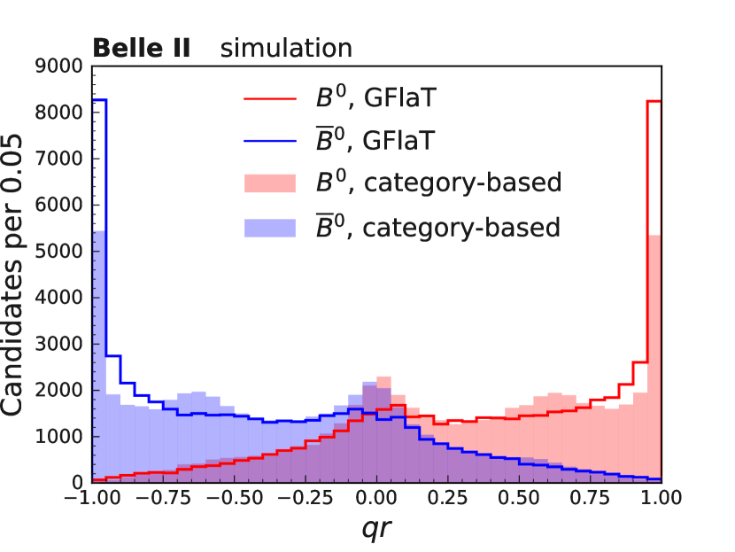
Figure 1 shows the qr𝑞𝑟qr distributions for true B0\mathit{{B}{}_{\mspace{-3.0mu}\scriptstyle{}}^{\mspace{-1.0mu}\scriptstyle{$0$}}} and B¯0\mathit{{\mkern 4.0mu\overline{\mkern-4.0mu{B}}}{}_{\mspace{-2.0mu}\scriptstyle{}}^{\mspace{0.0mu}\scriptstyle{$0$}}} for independent test data consisting of 1×1051E+51\text{\times}{10}^{5} events from GFlaT and the category-based flavor tagger. The latter has more reliable tagging information than reported in Ref. [14], due to recent improvements in particle identification and parameter tuning. GFlaT better distinguishes between B0\mathit{{B}{}_{\mspace{-3.0mu}\scriptstyle{}}^{\mspace{-1.0mu}\scriptstyle{$0$}}} and B¯0\mathit{{\mkern 4.0mu\overline{\mkern-4.0mu{B}}}{}_{\mspace{-2.0mu}\scriptstyle{}}^{\mspace{0.0mu}\scriptstyle{$0$}}} than the category-based flavor tagger: the peaks at |qr|1𝑞𝑟1|qr|\approx 1 are higher and the bumps at |qr|0𝑞𝑟0|qr|\approx 0 and |qr|0.65𝑞𝑟0.65|qr|\approx 0.65 are smaller.

Refer to caption
Figure 1: Distributions of qr𝑞𝑟qr for true B0\mathit{{B}{}_{\mspace{-3.0mu}\scriptstyle{}}^{\mspace{-1.0mu}\scriptstyle{$0$}}} and B¯0\mathit{{\mkern 4.0mu\overline{\mkern-4.0mu{B}}}{}_{\mspace{-2.0mu}\scriptstyle{}}^{\mspace{0.0mu}\scriptstyle{$0$}}} from GFlaT and the category-based flavor tagger in simulated data.

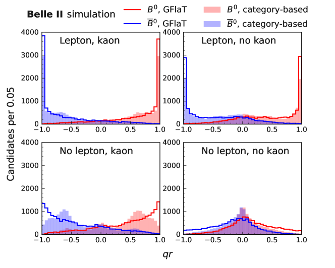
Figure 2 shows the qr𝑞𝑟qr distributions for events classified according to the presence of charged leptons or kaons in the ROE. The ROE contains a charged lepton and a charged kaon in 22.2% of events, a charged lepton and no charged kaon in 22.9%, a charged kaon and no charged lepton in 31.5%, and neither in 23.4%. The distributions indicate that performance is optimal when both a lepton and a kaon are present, with the contribution from leptons being particularly significant. The distributions also reveal that the bump at |qr|0.65𝑞𝑟0.65|qr|\approx 0.65 in the category-based flavor tagger is due to events with charged kaons, which indicates that flavor assignment in such events is less reliable since a K\mathit{{K}{}_{\mspace{-3.0mu}\scriptstyle{}}^{\mspace{-1.0mu}\scriptstyle{-}}}, predominantly associated with B¯0\mathit{{\mkern 4.0mu\overline{\mkern-4.0mu{B}}}{}_{\mspace{-2.0mu}\scriptstyle{}}^{\mspace{0.0mu}\scriptstyle{$0$}}} decays, can also originate from a B0\mathit{{B}{}_{\mspace{-3.0mu}\scriptstyle{}}^{\mspace{-1.0mu}\scriptstyle{$0$}}} decay, for example through decay to a D\mathit{{D}{}_{\mspace{-3.0mu}\scriptstyle{}}^{\mspace{-1.0mu}\scriptstyle{-}}} with DK¯K0\mathit{{D}{}_{\mspace{-3.0mu}\scriptstyle{}}^{\mspace{-1.0mu}\scriptstyle{-}}}\to\mathit{{\mkern 4.0mu\overline{\mkern-4.0mu{K}}}{}_{\mspace{-2.0mu}\scriptstyle{}}^{\mspace{0.0mu}\scriptstyle{$0$}}}\mathit{{K}{}_{\mspace{-3.0mu}\scriptstyle{}}^{\mspace{-1.0mu}\scriptstyle{-}}}. Since GFlaT accounts for the relationships between final-state particles, it can better discern the origin of the tracks; and so its output does not peak at |qr|0.65𝑞𝑟0.65|qr|\approx 0.65 for those events, but instead at |qr|1𝑞𝑟1|qr|\approx 1. Both flavor taggers perform poorly for events with neither a charged lepton nor a charged kaon, consisting mostly of pions, but GFlaT’s output still exhibits a visible improvement. A charged pion from B0\mathit{{B}{}_{\mspace{-3.0mu}\scriptstyle{}}^{\mspace{-1.0mu}\scriptstyle{$0$}}} decay, such as B0Dπ+\mathit{{B}{}_{\mspace{-3.0mu}\scriptstyle{}}^{\mspace{-1.0mu}\scriptstyle{$0$}}}\to\mathit{{D}{}_{\mspace{-3.0mu}\scriptstyle{}}^{\mspace{-1.0mu}\scriptstyle{-}}}\mathit{{\pi}{}_{\mspace{-3.0mu}\scriptstyle{}}^{\mspace{-1.0mu}\scriptstyle{+}}}, or through an intermediate resonance that decays via the strong force, correlates with the B\mathit{{B}{}_{\mspace{-3.0mu}\scriptstyle{}}^{\mspace{-1.0mu}\scriptstyle{}}} flavor. The GFlaT algorithm exploits this correlation more effectively to improve performance.
Refer to caption
Figure 2: Distributions of qr𝑞𝑟qr for true B0\mathit{{B}{}_{\mspace{-3.0mu}\scriptstyle{}}^{\mspace{-1.0mu}\scriptstyle{$0$}}} and B¯0\mathit{{\mkern 4.0mu\overline{\mkern-4.0mu{B}}}{}_{\mspace{-2.0mu}\scriptstyle{}}^{\mspace{0.0mu}\scriptstyle{$0$}}} from GFlaT and the category-based flavor tagger for events classified according to the presence of charged leptons or charged kaons in the ROE in simulation data.

IV Calibration and performance

We evaluate GFlaT’s performance using events in which Bsig\mathit{{B}{}_{\mspace{-3.0mu}\scriptstyle{\text{sig}}}^{\mspace{-1.0mu}\scriptstyle{}}} decays to the Dπ()+\mathit{{D}{}_{\mspace{-3.0mu}\scriptstyle{}}^{\mspace{-1.0mu}\scriptstyle{(*)-}}}\mathit{{\pi}{}_{\mspace{-3.0mu}\scriptstyle{}}^{\mspace{-1.0mu}\scriptstyle{+}}} final state. The flavor of Bsig\mathit{{B}{}_{\mspace{-3.0mu}\scriptstyle{\text{sig}}}^{\mspace{-1.0mu}\scriptstyle{}}} is determined by the charge of the pion, neglecting the wrong-sign contribution. We fit the ΔtΔ𝑡\Delta t probability density model to the background-subtracted ΔtΔ𝑡\Delta t distribution, accounting for resolution effects, to determine the wrong-tag probability w𝑤w in each r𝑟r bin. We subtract the background with sWeight [40, 41] using the B\mathit{{B}{}_{\mspace{-3.0mu}\scriptstyle{}}^{\mspace{-1.0mu}\scriptstyle{}}} energy as a discriminating variable.

We reconstruct D\mathit{{D}{}_{\mspace{-3.0mu}\scriptstyle{}}^{\mspace{-1.0mu}\scriptstyle{-}}} candidates via DKπ+π\mathit{{D}{}_{\mspace{-3.0mu}\scriptstyle{}}^{\mspace{-1.0mu}\scriptstyle{-}}}\to\mathit{{K}{}_{\mspace{-3.0mu}\scriptstyle{}}^{\mspace{-1.0mu}\scriptstyle{+}}}\mathit{{\pi}{}_{\mspace{-3.0mu}\scriptstyle{}}^{\mspace{-1.0mu}\scriptstyle{-}}}\mathit{{\pi}{}_{\mspace{-3.0mu}\scriptstyle{}}^{\mspace{-1.0mu}\scriptstyle{-}}} and via D¯π0\to\mathit{{\mkern 4.0mu\overline{\mkern-4.0mu{D}}}{}_{\mspace{-2.0mu}\scriptstyle{}}^{\mspace{0.0mu}\scriptstyle{$0$}}}\mathit{{\pi}{}_{\mspace{-3.0mu}\scriptstyle{}}^{\mspace{-1.0mu}\scriptstyle{-}}} with D¯0Kπ+\mathit{{\mkern 4.0mu\overline{\mkern-4.0mu{D}}}{}_{\mspace{-2.0mu}\scriptstyle{}}^{\mspace{0.0mu}\scriptstyle{$0$}}}\to\mathit{{K}{}_{\mspace{-3.0mu}\scriptstyle{}}^{\mspace{-1.0mu}\scriptstyle{+}}}\mathit{{\pi}{}_{\mspace{-3.0mu}\scriptstyle{}}^{\mspace{-1.0mu}\scriptstyle{-}}}, Kπ+π0\mathit{{K}{}_{\mspace{-3.0mu}\scriptstyle{}}^{\mspace{-1.0mu}\scriptstyle{+}}}\mathit{{\pi}{}_{\mspace{-3.0mu}\scriptstyle{}}^{\mspace{-1.0mu}\scriptstyle{-}}}\mathit{{\pi}{}_{\mspace{-3.0mu}\scriptstyle{}}^{\mspace{-1.0mu}\scriptstyle{$0$}}}, or Kπ+ππ+\mathit{{K}{}_{\mspace{-3.0mu}\scriptstyle{}}^{\mspace{-1.0mu}\scriptstyle{+}}}\mathit{{\pi}{}_{\mspace{-3.0mu}\scriptstyle{}}^{\mspace{-1.0mu}\scriptstyle{-}}}\mathit{{\pi}{}_{\mspace{-3.0mu}\scriptstyle{}}^{\mspace{-1.0mu}\scriptstyle{+}}}\mathit{{\pi}{}_{\mspace{-3.0mu}\scriptstyle{}}^{\mspace{-1.0mu}\scriptstyle{-}}}. Tracks must originate from the IR and have polar angles within the CDC.

We reconstruct π0\mathit{{\pi}{}_{\mspace{-3.0mu}\scriptstyle{}}^{\mspace{-1.0mu}\scriptstyle{$0$}}} candidates via π0γγ\mathit{{\pi}{}_{\mspace{-3.0mu}\scriptstyle{}}^{\mspace{-1.0mu}\scriptstyle{$0$}}}\to\mathit{{\gamma}{}_{\mspace{-3.0mu}\scriptstyle{}}^{\mspace{-1.0mu}\scriptstyle{}}}\mathit{{\gamma}{}_{\mspace{-3.0mu}\scriptstyle{}}^{\mspace{-1.0mu}\scriptstyle{}}}, forming photon candidates from ECL clusters not associated with any tracks. To suppress beam-background photons, we require each cluster have an energy greater than 120 MeVtimes120MeV120\text{\,}\mathrm{M}\mathrm{e}\mathrm{V}, 30 MeVtimes30MeV30\text{\,}\mathrm{M}\mathrm{e}\mathrm{V}, or 80 MeVtimes80MeV80\text{\,}\mathrm{M}\mathrm{e}\mathrm{V} if it is in the forward, barrel, or backward region of the ECL, which corresponds to the lab-frame polar angle ranges [12.4,31.4]°12.431.4degree[$12.4$,$31.4$]\,$\mathrm{\SIUnitSymbolDegree}$, [32.2,128.7]°32.2128.7degree[$32.2$,$128.7$]\,$\mathrm{\SIUnitSymbolDegree}$, and [130.7,155.1]°130.7155.1degree[$130.7$,$155.1$]\,$\mathrm{\SIUnitSymbolDegree}$, respectively. The angle between the photon momenta must be less than 52 °times52degree52\text{\,}\mathrm{\SIUnitSymbolDegree} in the lab frame and the diphoton mass must be in the range [121,142]MeV121142MeV[$121$,$142$]\,$\mathrm{M}\mathrm{e}\mathrm{V}$, which is centered on the known π0\mathit{{\pi}{}_{\mspace{-3.0mu}\scriptstyle{}}^{\mspace{-1.0mu}\scriptstyle{$0$}}} mass and is six units of diphoton mass resolution wide.

One of the D\mathit{{D}{}_{\mspace{-3.0mu}\scriptstyle{}}^{\mspace{-1.0mu}\scriptstyle{}}}’s decay products must be consistent with being a K+\mathit{{K}{}_{\mspace{-3.0mu}\scriptstyle{}}^{\mspace{-1.0mu}\scriptstyle{+}}}, but no particle-identification requirements are placed on the other charged particles. Each D\mathit{{D}{}_{\mspace{-3.0mu}\scriptstyle{}}^{\mspace{-1.0mu}\scriptstyle{-}}} candidate must have a mass in [1.860,1.880]GeV1.8601.880GeV[$1.860$,$1.880$]\,$\mathrm{G}\mathrm{e}\mathrm{V}$, which is centered on the known D\mathit{{D}{}_{\mspace{-3.0mu}\scriptstyle{}}^{\mspace{-1.0mu}\scriptstyle{-}}} mass and is a ±3σplus-or-minus3𝜎\pm 3\sigma range, with σ𝜎\sigma being the mass resolution. Each D¯0\mathit{{\mkern 4.0mu\overline{\mkern-4.0mu{D}}}{}_{\mspace{-2.0mu}\scriptstyle{}}^{\mspace{0.0mu}\scriptstyle{$0$}}} candidate reconstructed from Kπ+(ππ+)\mathit{{K}{}_{\mspace{-3.0mu}\scriptstyle{}}^{\mspace{-1.0mu}\scriptstyle{+}}}\mathit{{\pi}{}_{\mspace{-3.0mu}\scriptstyle{}}^{\mspace{-1.0mu}\scriptstyle{-}}}(\mathit{{\pi}{}_{\mspace{-3.0mu}\scriptstyle{}}^{\mspace{-1.0mu}\scriptstyle{+}}}\mathit{{\pi}{}_{\mspace{-3.0mu}\scriptstyle{}}^{\mspace{-1.0mu}\scriptstyle{-}}}) must have a mass in [1.845,1.885]GeV1.8451.885GeV[$1.845$,$1.885$]\,$\mathrm{G}\mathrm{e}\mathrm{V}$, which is centered on the known D¯0\mathit{{\mkern 4.0mu\overline{\mkern-4.0mu{D}}}{}_{\mspace{-2.0mu}\scriptstyle{}}^{\mspace{0.0mu}\scriptstyle{$0$}}} mass and is a ±5σplus-or-minus5𝜎\pm 5\sigma range. Each D¯0\mathit{{\mkern 4.0mu\overline{\mkern-4.0mu{D}}}{}_{\mspace{-2.0mu}\scriptstyle{}}^{\mspace{0.0mu}\scriptstyle{$0$}}} candidate reconstructed from Kπ+π0\mathit{{K}{}_{\mspace{-3.0mu}\scriptstyle{}}^{\mspace{-1.0mu}\scriptstyle{+}}}\mathit{{\pi}{}_{\mspace{-3.0mu}\scriptstyle{}}^{\mspace{-1.0mu}\scriptstyle{-}}}\mathit{{\pi}{}_{\mspace{-3.0mu}\scriptstyle{}}^{\mspace{-1.0mu}\scriptstyle{$0$}}} must have a mass in [1.810,1.895]GeV1.8101.895GeV[$1.810$,$1.895$]\,$\mathrm{G}\mathrm{e}\mathrm{V}$, which is an asymmetric range of +2.5σ2.5𝜎+2.5\sigma and 4σ4𝜎-4\sigma around the known D¯0\mathit{{\mkern 4.0mu\overline{\mkern-4.0mu{D}}}{}_{\mspace{-2.0mu}\scriptstyle{}}^{\mspace{0.0mu}\scriptstyle{$0$}}} mass to account for energy losses in photon reconstruction.

The π\mathit{{\pi}{}_{\mspace{-3.0mu}\scriptstyle{}}^{\mspace{-1.0mu}\scriptstyle{-}}} from a candidate decay must have momentum below 300 MeVtimes300MeV300\text{\,}\mathrm{M}\mathrm{e}\mathrm{V} in the ee+\mathit{{e}{}_{\mspace{-3.0mu}\scriptstyle{}}^{\mspace{-1.0mu}\scriptstyle{+}}}\mathit{{e}{}_{\mspace{-3.0mu}\scriptstyle{}}^{\mspace{-1.0mu}\scriptstyle{-}}} center-of-mass (c.m.) frame. Each candidate must have an energy release, m()m(D¯)0mπm()-m(\mathit{{\mkern 4.0mu\overline{\mkern-4.0mu{D}}}{}_{\mspace{-2.0mu}\scriptstyle{}}^{\mspace{0.0mu}\scriptstyle{$0$}}})-m_{\mathit{{\pi}{}_{\mspace{-3.0mu}\scriptstyle{}}^{\mspace{-1.0mu}\scriptstyle{-}}}}, in [4.6,7.0]MeV4.67.0MeV[$4.6$,$7.0$]\,$\mathrm{M}\mathrm{e}\mathrm{V}$, which is centered around the known energy release and six units of its resolution wide.

We reconstruct a B0\mathit{{B}{}_{\mspace{-3.0mu}\scriptstyle{}}^{\mspace{-1.0mu}\scriptstyle{$0$}}} candidate from a D()\mathit{{D}{}_{\mspace{-3.0mu}\scriptstyle{}}^{\mspace{-1.0mu}\scriptstyle{(*)-}}} candidate and a track that is consistent with being a π+\mathit{{\pi}{}_{\mspace{-3.0mu}\scriptstyle{}}^{\mspace{-1.0mu}\scriptstyle{+}}}. For each B0\mathit{{B}{}_{\mspace{-3.0mu}\scriptstyle{}}^{\mspace{-1.0mu}\scriptstyle{$0$}}} candidate, we fit the trajectories and momenta of its decay products according to its decay chain with TreeFit [42], constraining the B0\mathit{{B}{}_{\mspace{-3.0mu}\scriptstyle{}}^{\mspace{-1.0mu}\scriptstyle{$0$}}} to originate from the IR and the D()\mathit{{D}{}_{\mspace{-3.0mu}\scriptstyle{}}^{\mspace{-1.0mu}\scriptstyle{(*)}}} to its known mass [37]. We reject B0\mathit{{B}{}_{\mspace{-3.0mu}\scriptstyle{}}^{\mspace{-1.0mu}\scriptstyle{$0$}}} candidates whose fits do not converge. The fraction of rejected signal candidates is 0.4%. We define the signal region from a beam-constrained mass

MbcEbeam2|p|2subscript𝑀bcsuperscriptsubscript𝐸beam2superscript𝑝2M_{\text{bc}}\equiv\sqrt{E_{\text{beam}}^{2}-\absolutevalue*{\vec{p}}^{2}} (4)

and energy difference, ΔEEEbeamΔ𝐸𝐸subscript𝐸beam\Delta E\equiv E-E_{\text{beam}}, where Ebeamsubscript𝐸beamE_{\text{beam}}, E𝐸E, and p𝑝\vec{p} are the beam energy and B0\mathit{{B}{}_{\mspace{-3.0mu}\scriptstyle{}}^{\mspace{-1.0mu}\scriptstyle{$0$}}} energy and momentum in the c.m. frame, respectively. The criteria for the signal region are Mbc>5.27 GeVsubscript𝑀bctimes5.27GeVM_{\text{bc}}>$5.27\text{\,}\mathrm{G}\mathrm{e}\mathrm{V}$ and ΔE[0.10,0.25]GeVΔ𝐸-0.100.25GeV\Delta E\in[$-0.10$,$0.25$]\,$\mathrm{G}\mathrm{e}\mathrm{V}$.

We determine the decay position of Btag\mathit{{B}{}_{\mspace{-3.0mu}\scriptstyle{\text{tag}}}^{\mspace{-1.0mu}\scriptstyle{}}} by fitting the trajectories of ROE tracks with Rave [43]. Unlike TreeFit, Rave accounts for the unknown Btag\mathit{{B}{}_{\mspace{-3.0mu}\scriptstyle{\text{tag}}}^{\mspace{-1.0mu}\scriptstyle{}}} decay chain by reducing the impact of a displaced vertex due to potential intermediate D\mathit{{D}{}_{\mspace{-3.0mu}\scriptstyle{}}^{\mspace{-1.0mu}\scriptstyle{}}}’s, constraining the Btag\mathit{{B}{}_{\mspace{-3.0mu}\scriptstyle{\text{tag}}}^{\mspace{-1.0mu}\scriptstyle{}}} vertex position to be consistent with the origin and direction of Bsig\mathit{{B}{}_{\mspace{-3.0mu}\scriptstyle{\text{sig}}}^{\mspace{-1.0mu}\scriptstyle{}}}. We reject events in which this fit does not converge, which rejects 3.4% of the signal events.

To suppress events not coming from ee+BB¯\mathit{{e}{}_{\mspace{-3.0mu}\scriptstyle{}}^{\mspace{-1.0mu}\scriptstyle{+}}}\mathit{{e}{}_{\mspace{-3.0mu}\scriptstyle{}}^{\mspace{-1.0mu}\scriptstyle{-}}}\to\mathit{{B}{}_{\mspace{-3.0mu}\scriptstyle{}}^{\mspace{-1.0mu}\scriptstyle{}}}\mathit{{\mkern 4.0mu\overline{\mkern-4.0mu{B}}}{}_{\mspace{-2.0mu}\scriptstyle{}}^{\mspace{0.0mu}\scriptstyle{}}}, such as ee+qq¯\mathit{{e}{}_{\mspace{-3.0mu}\scriptstyle{}}^{\mspace{-1.0mu}\scriptstyle{+}}}\mathit{{e}{}_{\mspace{-3.0mu}\scriptstyle{}}^{\mspace{-1.0mu}\scriptstyle{-}}}\to\mathit{{q}{}_{\mspace{-3.0mu}\scriptstyle{}}^{\mspace{-1.0mu}\scriptstyle{}}}\mathit{{\mkern 4.0mu\overline{\mkern-4.0mu{q}}}{}_{\mspace{-2.0mu}\scriptstyle{}}^{\mspace{0.0mu}\scriptstyle{}}}, we exploit their topological differences, by requiring the ratio of the second to the zeroth Fox-Wolfram moment, R2subscript𝑅2R_{2}, be less than 0.40.40.4 [44]. After applying all selection requirements, the average number of candidates per event is 1.05 and all candidates are retained.

Events passing the above criteria are either correctly identified Bsig\mathit{{B}{}_{\mspace{-3.0mu}\scriptstyle{\text{sig}}}^{\mspace{-1.0mu}\scriptstyle{}}} decays or backgrounds from BB¯\mathit{{B}{}_{\mspace{-3.0mu}\scriptstyle{}}^{\mspace{-1.0mu}\scriptstyle{}}}\mathit{{\mkern 4.0mu\overline{\mkern-4.0mu{B}}}{}_{\mspace{-2.0mu}\scriptstyle{}}^{\mspace{0.0mu}\scriptstyle{}}} and qq¯\mathit{{q}{}_{\mspace{-3.0mu}\scriptstyle{}}^{\mspace{-1.0mu}\scriptstyle{}}}\mathit{{\mkern 4.0mu\overline{\mkern-4.0mu{q}}}{}_{\mspace{-2.0mu}\scriptstyle{}}^{\mspace{0.0mu}\scriptstyle{}}} events. To separate signal from background, we fit to the ΔEΔ𝐸\Delta E distribution using an extended unbinned likelihood, combining data from Bsig\mathit{{B}{}_{\mspace{-3.0mu}\scriptstyle{\text{sig}}}^{\mspace{-1.0mu}\scriptstyle{}}} and B¯sig\mathit{{\mkern 4.0mu\overline{\mkern-4.0mu{B}}}{}_{\mspace{-2.0mu}\scriptstyle{\text{sig}}}^{\mspace{0.0mu}\scriptstyle{}}} and all r𝑟r intervals.

We model the signal contribution as the sum of a Gaussian function and a double-sided Crystal-Ball function [45]. Their parameters and their admixture are fixed to values obtained from fitting to simulated data, but a common shift of their peak values and common scaling of their widths are left free to account for differences between data and simulation.

Events in which Bsig\mathit{{B}{}_{\mspace{-3.0mu}\scriptstyle{\text{sig}}}^{\mspace{-1.0mu}\scriptstyle{}}} decays to the DK()+\mathit{{D}{}_{\mspace{-3.0mu}\scriptstyle{}}^{\mspace{-1.0mu}\scriptstyle{(*)-}}}\mathit{{K}{}_{\mspace{-3.0mu}\scriptstyle{}}^{\mspace{-1.0mu}\scriptstyle{+}}} final state, with the K+\mathit{{K}{}_{\mspace{-3.0mu}\scriptstyle{}}^{\mspace{-1.0mu}\scriptstyle{+}}} misidentified as a π+\mathit{{\pi}{}_{\mspace{-3.0mu}\scriptstyle{}}^{\mspace{-1.0mu}\scriptstyle{+}}}, peak at 50 MeVtimes-50MeV-50\text{\,}\mathrm{M}\mathrm{e}\mathrm{V} in the ΔEΔ𝐸\Delta E distribution. According to simulation studies, the fraction of these events to the signal is 2.5%percent2.52.5\%. We model this contribution as a double-sided Crystal Ball function, whose parameters are fixed to values obtained from fitting to simulated data, including the ratio of its yield to the signal, except for the shift of its peak value and the scaling of its width, which are the same as for the signal. Since these events have the same ΔtΔ𝑡\Delta t distribution as B0Dπ()+\mathit{{B}{}_{\mspace{-3.0mu}\scriptstyle{}}^{\mspace{-1.0mu}\scriptstyle{$0$}}}\to\mathit{{D}{}_{\mspace{-3.0mu}\scriptstyle{}}^{\mspace{-1.0mu}\scriptstyle{(*)-}}}\mathit{{\pi}{}_{\mspace{-3.0mu}\scriptstyle{}}^{\mspace{-1.0mu}\scriptstyle{+}}}, we use this contribution as signal in the sWeight calculation.

We model the BB¯\mathit{{B}{}_{\mspace{-3.0mu}\scriptstyle{}}^{\mspace{-1.0mu}\scriptstyle{}}}\mathit{{\mkern 4.0mu\overline{\mkern-4.0mu{B}}}{}_{\mspace{-2.0mu}\scriptstyle{}}^{\mspace{0.0mu}\scriptstyle{}}} background contribution as a second-order polynomial, with the ratio of its yield to that of the signal fixed to a value obtained from simulated data. We model the qq¯\mathit{{q}{}_{\mspace{-3.0mu}\scriptstyle{}}^{\mspace{-1.0mu}\scriptstyle{}}}\mathit{{\mkern 4.0mu\overline{\mkern-4.0mu{q}}}{}_{\mspace{-2.0mu}\scriptstyle{}}^{\mspace{0.0mu}\scriptstyle{}}} background contribution as an exponential function. To constrain the parameters of the qq¯\mathit{{q}{}_{\mspace{-3.0mu}\scriptstyle{}}^{\mspace{-1.0mu}\scriptstyle{}}}\mathit{{\mkern 4.0mu\overline{\mkern-4.0mu{q}}}{}_{\mspace{-2.0mu}\scriptstyle{}}^{\mspace{0.0mu}\scriptstyle{}}} component, we simultaneously fit to the ΔEΔ𝐸\Delta E distribution in a sideband, Mbc[5.20,5.24]GeVsubscript𝑀bc5.205.24GeVM_{\text{bc}}\in[$5.20$,$5.24$]\,$\mathrm{G}\mathrm{e}\mathrm{V}$, populated predominantly by qq¯\mathit{{q}{}_{\mspace{-3.0mu}\scriptstyle{}}^{\mspace{-1.0mu}\scriptstyle{}}}\mathit{{\mkern 4.0mu\overline{\mkern-4.0mu{q}}}{}_{\mspace{-2.0mu}\scriptstyle{}}^{\mspace{0.0mu}\scriptstyle{}}} events. We confirm via simulation studies that the ΔEΔ𝐸\Delta E distributions of the qq¯\mathit{{q}{}_{\mspace{-3.0mu}\scriptstyle{}}^{\mspace{-1.0mu}\scriptstyle{}}}\mathit{{\mkern 4.0mu\overline{\mkern-4.0mu{q}}}{}_{\mspace{-2.0mu}\scriptstyle{}}^{\mspace{0.0mu}\scriptstyle{}}} component in the signal and sideband regions are sufficiently similar to warrant a simultaneous fit.

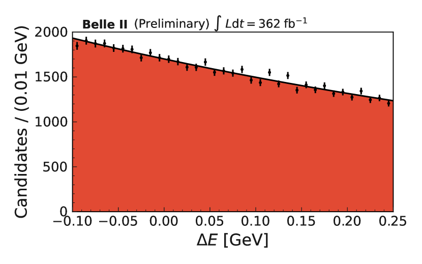
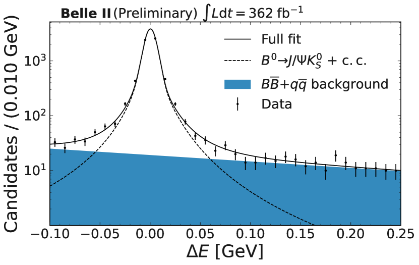
Figure 3 shows the ΔEΔ𝐸\Delta E distributions in the signal region and sideband and the fit results. The fit agrees well with the data. Yields in the signal region are 77 130±320uncertain7713032077\,130\pm 320 events for the signal (for the sum of the Dπ()+\mathit{{D}{}_{\mspace{-3.0mu}\scriptstyle{}}^{\mspace{-1.0mu}\scriptstyle{(*)-}}}\mathit{{\pi}{}_{\mspace{-3.0mu}\scriptstyle{}}^{\mspace{-1.0mu}\scriptstyle{+}}} and DK()+\mathit{{D}{}_{\mspace{-3.0mu}\scriptstyle{}}^{\mspace{-1.0mu}\scriptstyle{(*)-}}}\mathit{{K}{}_{\mspace{-3.0mu}\scriptstyle{}}^{\mspace{-1.0mu}\scriptstyle{+}}} final states), 8620±40uncertain8620408620\pm 40 for the BB¯\mathit{{B}{}_{\mspace{-3.0mu}\scriptstyle{}}^{\mspace{-1.0mu}\scriptstyle{}}}\mathit{{\mkern 4.0mu\overline{\mkern-4.0mu{B}}}{}_{\mspace{-2.0mu}\scriptstyle{}}^{\mspace{0.0mu}\scriptstyle{}}} background, and 14 200±230uncertain1420023014\,200\pm 230 for the qq¯\mathit{{q}{}_{\mspace{-3.0mu}\scriptstyle{}}^{\mspace{-1.0mu}\scriptstyle{}}}\mathit{{\mkern 4.0mu\overline{\mkern-4.0mu{q}}}{}_{\mspace{-2.0mu}\scriptstyle{}}^{\mspace{0.0mu}\scriptstyle{}}} background.

Refer to caption
Refer to caption
Figure 3: Distributions of ΔEΔ𝐸\Delta E for B0Dπ()+\mathit{{B}{}_{\mspace{-3.0mu}\scriptstyle{}}^{\mspace{-1.0mu}\scriptstyle{$0$}}}\to\mathit{{D}{}_{\mspace{-3.0mu}\scriptstyle{}}^{\mspace{-1.0mu}\scriptstyle{(*)-}}}\mathit{{\pi}{}_{\mspace{-3.0mu}\scriptstyle{}}^{\mspace{-1.0mu}\scriptstyle{+}}} reconstructed in data in the signal region (top) and sideband (bottom) and the best-fit function, with background components stacked.

We modify equation (2) to account for differences in the wrong-tag probabilities for Btag\mathit{{B}{}_{\mspace{-3.0mu}\scriptstyle{\text{tag}}}^{\mspace{-1.0mu}\scriptstyle{}}} and B¯tag\mathit{{\mkern 4.0mu\overline{\mkern-4.0mu{B}}}{}_{\mspace{-2.0mu}\scriptstyle{\text{tag}}}^{\mspace{0.0mu}\scriptstyle{}}}, by introducing w(B)0w¯+12Δww(\mathit{{B}{}_{\mspace{-3.0mu}\scriptstyle{}}^{\mspace{-1.0mu}\scriptstyle{$0$}}})\equiv\bar{w}+\tfrac{1}{2}\Delta w and w(B¯)0w¯12Δww(\mathit{{\mkern 4.0mu\overline{\mkern-4.0mu{B}}}{}_{\mspace{-2.0mu}\scriptstyle{}}^{\mspace{0.0mu}\scriptstyle{$0$}}})\equiv\bar{w}-\tfrac{1}{2}\Delta w and reconstruction efficiency asymmetries for Bsig\mathit{{B}{}_{\mspace{-3.0mu}\scriptstyle{\text{sig}}}^{\mspace{-1.0mu}\scriptstyle{}}} and Btag\mathit{{B}{}_{\mspace{-3.0mu}\scriptstyle{\text{tag}}}^{\mspace{-1.0mu}\scriptstyle{}}}, asigsubscript𝑎siga_{\text{sig}} and atagsubscript𝑎taga_{\text{tag}}, with ax[ε(B)x0ε(B¯)x0]/[ε(B¯)x0+ε(B¯)x0]a_{x}\equiv[\varepsilon(\mathit{{B}{}_{\mspace{-3.0mu}\scriptstyle{x}}^{\mspace{-1.0mu}\scriptstyle{$0$}}})-\varepsilon(\mathit{{\mkern 4.0mu\overline{\mkern-4.0mu{B}}}{}_{\mspace{-2.0mu}\scriptstyle{x}}^{\mspace{0.0mu}\scriptstyle{$0$}}})]/[\varepsilon(\mathit{{\mkern 4.0mu\overline{\mkern-4.0mu{B}}}{}_{\mspace{-2.0mu}\scriptstyle{x}}^{\mspace{0.0mu}\scriptstyle{$0$}}})+\varepsilon(\mathit{{\mkern 4.0mu\overline{\mkern-4.0mu{B}}}{}_{\mspace{-2.0mu}\scriptstyle{x}}^{\mspace{0.0mu}\scriptstyle{$0$}}})], where x𝑥x indicates ‘tag’ or ‘sig’,

P(Δt,qsig,qtag)=𝑃Δ𝑡subscript𝑞sigsubscript𝑞tagabsent\displaystyle P(\Delta t,q_{\text{sig}},q_{\text{tag}})=
(1+asigqsig)e|Δt|/τ4τ{1+qtag[atag(12w¯)Δw]\displaystyle\leavevmode\nobreak\ (1+a_{\text{sig}}q_{\text{sig}})\frac{e^{-\absolutevalue*{\Delta t}/\tau}}{4\tau}\big{\{}1+q_{\text{tag}}[a_{\text{tag}}(1-2\bar{w})-\Delta w]
+qsigqtag(12w¯+qtagatagatagΔw)cos(ΔmdΔt)}.\displaystyle\leavevmode\nobreak\ +q_{\text{sig}}q_{\text{tag}}\quantity(1-2\bar{w}+q_{\text{tag}}a_{\text{tag}}-a_{\text{tag}}\Delta w)\cos(\Delta m_{\mathit{{d}{}_{\mspace{-3.0mu}\scriptstyle{}}^{\mspace{-1.0mu}\scriptstyle{}}}}\Delta t)\big{\}}. (5)

We determine asigsubscript𝑎siga_{\text{sig}} by fitting the ΔEΔ𝐸\Delta E distributions for Bsig\mathit{{B}{}_{\mspace{-3.0mu}\scriptstyle{\text{sig}}}^{\mspace{-1.0mu}\scriptstyle{}}} and B¯sig\mathit{{\mkern 4.0mu\overline{\mkern-4.0mu{B}}}{}_{\mspace{-2.0mu}\scriptstyle{\text{sig}}}^{\mspace{0.0mu}\scriptstyle{}}} separately, using the same model as for their combined fit, without selection criteria on Btag\mathit{{B}{}_{\mspace{-3.0mu}\scriptstyle{\text{tag}}}^{\mspace{-1.0mu}\scriptstyle{}}} to avoid a bias from using Btag\mathit{{B}{}_{\mspace{-3.0mu}\scriptstyle{\text{tag}}}^{\mspace{-1.0mu}\scriptstyle{}}} information. We measure asigsubscript𝑎siga_{\text{sig}} = 2.53±0.39 %timesuncertain-2.530.39percent-2.53\pm 0.39\text{\,}\mathrm{\char 37\relax}, which we attribute to charge asymmetries in kaon identification and low-momentum track finding.

We calculate a per-candidate signal probability using sWeight from the ΔEΔ𝐸\Delta E-fit results, allowing us to statistically subtract background contributions to the ΔtΔ𝑡\Delta t distributions. This requires that ΔEΔ𝐸\Delta E, ΔtΔ𝑡\Delta t, and r𝑟r be independent, which is confirmed in simulation studies.

We calculate ΔtΔ𝑡\Delta t from the distance, ΔΔ\Delta\ell, of the Bsig\mathit{{B}{}_{\mspace{-3.0mu}\scriptstyle{\text{sig}}}^{\mspace{-1.0mu}\scriptstyle{}}} vertex from that of Btag\mathit{{B}{}_{\mspace{-3.0mu}\scriptstyle{\text{tag}}}^{\mspace{-1.0mu}\scriptstyle{}}} along the Υ(4S)\mathit{{\Upsilon}{}_{\mspace{-3.0mu}\scriptstyle{}}^{\mspace{-1.0mu}\scriptstyle{}}}{(4S)} boost direction,

Δt=ΔβγγB,\Delta t=\frac{\Delta\ell}{\beta\gamma\,\gamma_{\mathit{{B}{}_{\mspace{-3.0mu}\scriptstyle{}}^{\mspace{-1.0mu}\scriptstyle{}}}}}, (6)

where βγ=0.28𝛽𝛾0.28\beta\gamma=0.28 is the Lorentz boost of the Υ(4S)\mathit{{\Upsilon}{}_{\mspace{-3.0mu}\scriptstyle{}}^{\mspace{-1.0mu}\scriptstyle{}}}{(4S)} in the lab frame and γB=1.002\gamma_{\mathit{{B}{}_{\mspace{-3.0mu}\scriptstyle{}}^{\mspace{-1.0mu}\scriptstyle{}}}}=1.002 is the Lorentz factor of the B\mathit{{B}{}_{\mspace{-3.0mu}\scriptstyle{}}^{\mspace{-1.0mu}\scriptstyle{}}} in the c.m. frame.

To account for resolution and bias in measuring ΔΔ\Delta\ell, we convolve equation (5) with the resolution function introduced in Ref. [15]. The resolution function consists of a core component modeled by a Gaussian function, a tail component modeled by a weighted sum of a Gaussian and two exponentially modified Gaussian functions, and an outlier component modeled by a Gaussian function. Parameters of the resolution function are shared by all r𝑟r bins, except for the highest r𝑟r bin. This bin is mostly populated by semileptonic Btag\mathit{{B}{}_{\mspace{-3.0mu}\scriptstyle{\text{tag}}}^{\mspace{-1.0mu}\scriptstyle{}}} decays, which have a better resolution.

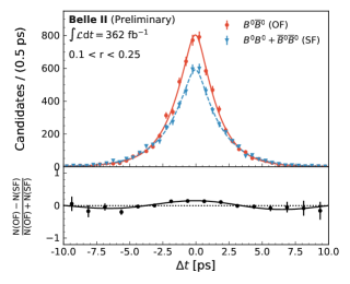
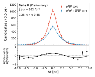
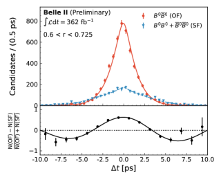
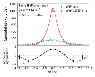
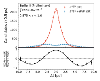
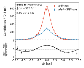
We fit simultaneously to the binned background-subtracted ΔtΔ𝑡\Delta t distributions in 28 subsets of the data defined by the 7 r𝑟r intervals, 2 flavors of Bsig\mathit{{B}{}_{\mspace{-3.0mu}\scriptstyle{\text{sig}}}^{\mspace{-1.0mu}\scriptstyle{}}}, and 2 flavors of Btag\mathit{{B}{}_{\mspace{-3.0mu}\scriptstyle{\text{tag}}}^{\mspace{-1.0mu}\scriptstyle{}}}. The fit has seven free resolution-function parameters and 21 free flavor-tagger parameters, atagsubscript𝑎taga_{\text{tag}}, w¯¯𝑤\bar{w}, and ΔwΔ𝑤\Delta w in each of the 7 r𝑟r bins. The uncertainty on the ΔtΔ𝑡\Delta t measurement, σΔtsubscript𝜎Δ𝑡\sigma_{\Delta t}, is computed for each event and is a conditional variable in the resolution function. We use a histogram with 500 bins in each data subset as the probability density function for this variable. We fix Δmd\Delta m_{\mathit{{d}{}_{\mspace{-3.0mu}\scriptstyle{}}^{\mspace{-1.0mu}\scriptstyle{}}}} and τ𝜏\tau to their world average values [37]. Figure 4 shows the ΔtΔ𝑡\Delta t distribution in each r𝑟r interval and the result of the fit.
Refer to caption
Refer to caption
Refer to caption
Refer to caption
Refer to caption
Refer to caption
Refer to caption
Figure 4: Background-subtracted ΔtΔ𝑡\Delta t distributions of B0Dπ()+\mathit{{B}{}_{\mspace{-3.0mu}\scriptstyle{}}^{\mspace{-1.0mu}\scriptstyle{$0$}}}\to\mathit{{D}{}_{\mspace{-3.0mu}\scriptstyle{}}^{\mspace{-1.0mu}\scriptstyle{(*)-}}}\mathit{{\pi}{}_{\mspace{-3.0mu}\scriptstyle{}}^{\mspace{-1.0mu}\scriptstyle{+}}} reconstructed in data in each of the seven r𝑟r intervals (points) and the best-fit functions (lines) for opposite- and like-flavor B\mathit{{B}{}_{\mspace{-3.0mu}\scriptstyle{}}^{\mspace{-1.0mu}\scriptstyle{}}} pairs with the corresponding asymmetries.

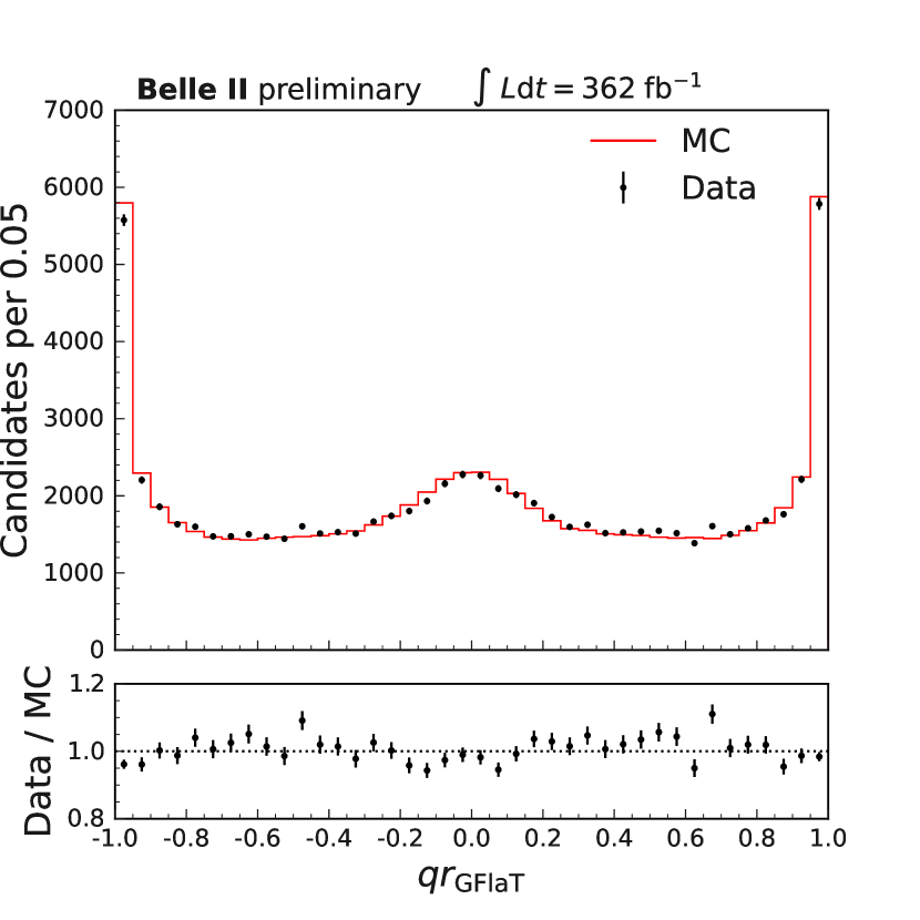
Figure 5 shows the qr​GFlaT𝑞subscript𝑟​GFlaTqr_{\text{\!GFlaT}} distribution in background-subtracted data and correctly reconstructed simulated events normalized to the data signal yield. Figure 6 shows the dilution factors, 12wi12subscript𝑤𝑖1-2w_{i}, for each r𝑟r bin i𝑖i for both Btag0\mathit{{B}{}_{\mspace{-3.0mu}\scriptstyle{\text{tag}}}^{\mspace{-1.0mu}\scriptstyle{$0$}}} and B¯tag0\mathit{{\mkern 4.0mu\overline{\mkern-4.0mu{B}}}{}_{\mspace{-2.0mu}\scriptstyle{\text{tag}}}^{\mspace{0.0mu}\scriptstyle{$0$}}}. It shows that r𝑟r is a good estimator of 12w12𝑤1-2w for both tag flavors. The effective tagging efficiency is εtag=(37.40±0.43)%subscript𝜀tagpercentuncertain37.400.43\varepsilon_{\text{tag}}=($37.40\pm 0.43$)\%, where the uncertainty is statistical only. Table 2 in Appendix A lists atagsubscript𝑎taga_{\text{tag}}, w¯¯𝑤\bar{w}, and ΔwΔ𝑤\Delta w for each r𝑟r bin.

Refer to caption
Figure 5: Distributions of qr​GFlaT𝑞subscript𝑟​GFlaTqr_{\text{\!GFlaT}} for B0Dπ()+\mathit{{B}{}_{\mspace{-3.0mu}\scriptstyle{}}^{\mspace{-1.0mu}\scriptstyle{$0$}}}\to\mathit{{D}{}_{\mspace{-3.0mu}\scriptstyle{}}^{\mspace{-1.0mu}\scriptstyle{(*)-}}}\mathit{{\pi}{}_{\mspace{-3.0mu}\scriptstyle{}}^{\mspace{-1.0mu}\scriptstyle{+}}} in background-subtracted data and correctly reconstructed simulated events normalized to the data signal yield.
Refer to caption
Figure 6: Dilution factors 12w12𝑤1-2w of B0Dπ()+\mathit{{B}{}_{\mspace{-3.0mu}\scriptstyle{}}^{\mspace{-1.0mu}\scriptstyle{$0$}}}\to\mathit{{D}{}_{\mspace{-3.0mu}\scriptstyle{}}^{\mspace{-1.0mu}\scriptstyle{(*)-}}}\mathit{{\pi}{}_{\mspace{-3.0mu}\scriptstyle{}}^{\mspace{-1.0mu}\scriptstyle{+}}} as functions of their GFlaT predictions, r𝑟r for Btag0\mathit{{B}{}_{\mspace{-3.0mu}\scriptstyle{\text{tag}}}^{\mspace{-1.0mu}\scriptstyle{$0$}}}, 12w¯Δw12¯𝑤Δ𝑤1-2\bar{w}-\Delta w, and B¯tag0\mathit{{\mkern 4.0mu\overline{\mkern-4.0mu{B}}}{}_{\mspace{-2.0mu}\scriptstyle{\text{tag}}}^{\mspace{0.0mu}\scriptstyle{$0$}}}, 12w¯+Δw12¯𝑤Δ𝑤1-2\bar{w}+\Delta w; the dashed line shows r=12w𝑟12𝑤r=1-2w.

V Measurement of sin2ϕ12subscriptitalic-ϕ1\sin 2\phi_{1} in B0J/ψKS0\mathit{{B}{}_{\mspace{-3.0mu}\scriptstyle{}}^{\mspace{-1.0mu}\scriptstyle{$0$}}}\to\mathit{{J\mspace{-2.0mu}/\mspace{-2.0mu}\psi}{}_{\mspace{-3.0mu}\scriptstyle{}}^{\mspace{-1.0mu}\scriptstyle{}}}\mathit{{K}{}_{\mspace{-3.0mu}\scriptstyle{\text{S}}}^{\mspace{-1.0mu}\scriptstyle{$0$}}}

We demonstrate GFlaT by measuring S𝑆S and C𝐶C in B0J/ψKS0\mathit{{B}{}_{\mspace{-3.0mu}\scriptstyle{}}^{\mspace{-1.0mu}\scriptstyle{$0$}}}\to\mathit{{J\mspace{-2.0mu}/\mspace{-2.0mu}\psi}{}_{\mspace{-3.0mu}\scriptstyle{}}^{\mspace{-1.0mu}\scriptstyle{}}}\mathit{{K}{}_{\mspace{-3.0mu}\scriptstyle{\text{S}}}^{\mspace{-1.0mu}\scriptstyle{$0$}}} decays. We reconstruct J/ψ\mathit{{J\mspace{-2.0mu}/\mspace{-2.0mu}\psi}{}_{\mspace{-3.0mu}\scriptstyle{}}^{\mspace{-1.0mu}\scriptstyle{}}} candidates via J/ψee+\mathit{{J\mspace{-2.0mu}/\mspace{-2.0mu}\psi}{}_{\mspace{-3.0mu}\scriptstyle{}}^{\mspace{-1.0mu}\scriptstyle{}}}\to\mathit{{e}{}_{\mspace{-3.0mu}\scriptstyle{}}^{\mspace{-1.0mu}\scriptstyle{+}}}\mathit{{e}{}_{\mspace{-3.0mu}\scriptstyle{}}^{\mspace{-1.0mu}\scriptstyle{-}}} or μμ+\mathit{{\mu}{}_{\mspace{-3.0mu}\scriptstyle{}}^{\mspace{-1.0mu}\scriptstyle{+}}}\mathit{{\mu}{}_{\mspace{-3.0mu}\scriptstyle{}}^{\mspace{-1.0mu}\scriptstyle{-}}}. The leptons must fulfill the same track requirements as described for the decay products of B0Dπ()+\mathit{{B}{}_{\mspace{-3.0mu}\scriptstyle{}}^{\mspace{-1.0mu}\scriptstyle{$0$}}}\to\mathit{{D}{}_{\mspace{-3.0mu}\scriptstyle{}}^{\mspace{-1.0mu}\scriptstyle{(*)-}}}\mathit{{\pi}{}_{\mspace{-3.0mu}\scriptstyle{}}^{\mspace{-1.0mu}\scriptstyle{+}}} and be consistent with both being electrons or both being muons. To account for energy loss due to bremsstrahlung, the four-momenta of photons with lab-frame energy in [75,1000]MeV751000MeV[$75$,$1000$]\,$\mathrm{M}\mathrm{e}\mathrm{V}$ detected within 50 mradtimes50mrad50\text{\,}\mathrm{m}\mathrm{r}\mathrm{a}\mathrm{d} of the initial direction of an electron are added to the electron’s four-momentum. Each J/ψee+\mathit{{J\mspace{-2.0mu}/\mspace{-2.0mu}\psi}{}_{\mspace{-3.0mu}\scriptstyle{}}^{\mspace{-1.0mu}\scriptstyle{}}}\to\mathit{{e}{}_{\mspace{-3.0mu}\scriptstyle{}}^{\mspace{-1.0mu}\scriptstyle{+}}}\mathit{{e}{}_{\mspace{-3.0mu}\scriptstyle{}}^{\mspace{-1.0mu}\scriptstyle{-}}} candidate must have a mass in [2.90,3.14]GeV2.903.14GeV[$2.90$,$3.14$]\,$\mathrm{G}\mathrm{e}\mathrm{V}$; each J/ψμμ+\mathit{{J\mspace{-2.0mu}/\mspace{-2.0mu}\psi}{}_{\mspace{-3.0mu}\scriptstyle{}}^{\mspace{-1.0mu}\scriptstyle{}}}\to\mathit{{\mu}{}_{\mspace{-3.0mu}\scriptstyle{}}^{\mspace{-1.0mu}\scriptstyle{+}}}\mathit{{\mu}{}_{\mspace{-3.0mu}\scriptstyle{}}^{\mspace{-1.0mu}\scriptstyle{-}}} candidate must have a mass in [3.00,3.14]GeV3.003.14GeV[$3.00$,$3.14$]\,$\mathrm{G}\mathrm{e}\mathrm{V}$. The resolutions at masses above and below the known J/ψ\mathit{{J\mspace{-2.0mu}/\mspace{-2.0mu}\psi}{}_{\mspace{-3.0mu}\scriptstyle{}}^{\mspace{-1.0mu}\scriptstyle{}}} mass are 8.0 MeVtimes8.0MeV8.0\text{\,}\mathrm{M}\mathrm{e}\mathrm{V} and 9.0 MeVtimes9.0MeV9.0\text{\,}\mathrm{M}\mathrm{e}\mathrm{V} for electron pairs and 6.3 MeVtimes6.3MeV6.3\text{\,}\mathrm{M}\mathrm{e}\mathrm{V} and 8.3 MeVtimes8.3MeV8.3\text{\,}\mathrm{M}\mathrm{e}\mathrm{V} for muon pairs.

We reconstruct KS0\mathit{{K}{}_{\mspace{-3.0mu}\scriptstyle{\text{S}}}^{\mspace{-1.0mu}\scriptstyle{$0$}}} candidates via KS0ππ+\mathit{{K}{}_{\mspace{-3.0mu}\scriptstyle{\text{S}}}^{\mspace{-1.0mu}\scriptstyle{$0$}}}\to\mathit{{\pi}{}_{\mspace{-3.0mu}\scriptstyle{}}^{\mspace{-1.0mu}\scriptstyle{+}}}\mathit{{\pi}{}_{\mspace{-3.0mu}\scriptstyle{}}^{\mspace{-1.0mu}\scriptstyle{-}}}. The pions must have polar angles within the CDC. Each KS0\mathit{{K}{}_{\mspace{-3.0mu}\scriptstyle{\text{S}}}^{\mspace{-1.0mu}\scriptstyle{$0$}}} candidate must have a mass in the range [0.45,0.55]GeV0.450.55GeV[$0.45$,$0.55$]\,$\mathrm{G}\mathrm{e}\mathrm{V}$, a successful vertex fit, and a decay vertex displaced from the IR by at least five units of the displacement’s uncertainty. The reconstructed KS0\mathit{{K}{}_{\mspace{-3.0mu}\scriptstyle{\text{S}}}^{\mspace{-1.0mu}\scriptstyle{$0$}}} mass resolution is 2.0 MeVtimes2.0MeV2.0\text{\,}\mathrm{M}\mathrm{e}\mathrm{V}.

We fit the trajectories and momenta of B0\mathit{{B}{}_{\mspace{-3.0mu}\scriptstyle{}}^{\mspace{-1.0mu}\scriptstyle{$0$}}} decay products with TreeFit, constraining the B0\mathit{{B}{}_{\mspace{-3.0mu}\scriptstyle{}}^{\mspace{-1.0mu}\scriptstyle{$0$}}} to originate from the IR and the J/ψ\mathit{{J\mspace{-2.0mu}/\mspace{-2.0mu}\psi}{}_{\mspace{-3.0mu}\scriptstyle{}}^{\mspace{-1.0mu}\scriptstyle{}}} to have its known mass [37]. Each B0\mathit{{B}{}_{\mspace{-3.0mu}\scriptstyle{}}^{\mspace{-1.0mu}\scriptstyle{$0$}}} candidate must have Mbcsubscript𝑀bcM_{\text{bc}} greater than 5.27 GeVtimes5.27GeV5.27\text{\,}\mathrm{G}\mathrm{e}\mathrm{V} and ΔEΔ𝐸\Delta E in [0.10,0.25]GeV-0.100.25GeV[$-0.10$,$0.25$]\,$\mathrm{G}\mathrm{e}\mathrm{V}$. The Btag\mathit{{B}{}_{\mspace{-3.0mu}\scriptstyle{\text{tag}}}^{\mspace{-1.0mu}\scriptstyle{}}} vertex position is determined as described for Bsig0Dπ()+\mathit{{B}{}_{\mspace{-3.0mu}\scriptstyle{\text{sig}}}^{\mspace{-1.0mu}\scriptstyle{$0$}}}\to\mathit{{D}{}_{\mspace{-3.0mu}\scriptstyle{}}^{\mspace{-1.0mu}\scriptstyle{(*)-}}}\mathit{{\pi}{}_{\mspace{-3.0mu}\scriptstyle{}}^{\mspace{-1.0mu}\scriptstyle{+}}} above. We require R2subscript𝑅2R_{2} be less than 0.4 to remove qq¯\mathit{{q}{}_{\mspace{-3.0mu}\scriptstyle{}}^{\mspace{-1.0mu}\scriptstyle{}}}\mathit{{\mkern 4.0mu\overline{\mkern-4.0mu{q}}}{}_{\mspace{-2.0mu}\scriptstyle{}}^{\mspace{0.0mu}\scriptstyle{}}} background. After applying all selection requirements, the average number of candidates per event is 1.01. All candidates are retained for further analysis.

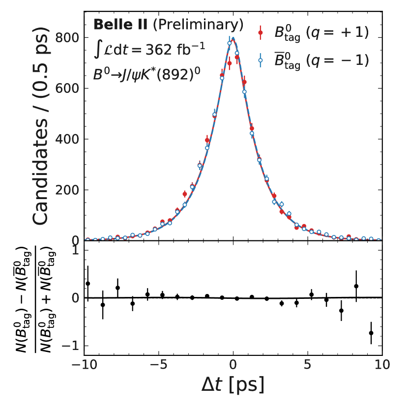
To validate our analysis, we also measure S𝑆S and C𝐶C for B0J/ψK(892)0\mathit{{B}{}_{\mspace{-3.0mu}\scriptstyle{}}^{\mspace{-1.0mu}\scriptstyle{$0$}}}\to\mathit{{J\mspace{-2.0mu}/\mspace{-2.0mu}\psi}{}_{\mspace{-3.0mu}\scriptstyle{}}^{\mspace{-1.0mu}\scriptstyle{}}}\mathit{{K}{}_{\mspace{-3.0mu}\scriptstyle{}}^{\mspace{-1.0mu}\scriptstyle{\ast}}}(892)^{0}, for which we expect S=0𝑆0S=0, as this decay mode is flavor-specific, and C=0𝐶0C=0 as with B0J/ψKS0\mathit{{B}{}_{\mspace{-3.0mu}\scriptstyle{}}^{\mspace{-1.0mu}\scriptstyle{$0$}}}\to\mathit{{J\mspace{-2.0mu}/\mspace{-2.0mu}\psi}{}_{\mspace{-3.0mu}\scriptstyle{}}^{\mspace{-1.0mu}\scriptstyle{}}}\mathit{{K}{}_{\mspace{-3.0mu}\scriptstyle{\text{S}}}^{\mspace{-1.0mu}\scriptstyle{$0$}}}. Hereafter, K(892)0\mathit{{K}{}_{\mspace{-3.0mu}\scriptstyle{}}^{\mspace{-1.0mu}\scriptstyle{\ast}}}(892)^{0} is written as K0\mathit{{K}{}_{\mspace{-3.0mu}\scriptstyle{}}^{\mspace{-1.0mu}\scriptstyle{*$0$}}}. We reconstruct K0\mathit{{K}{}_{\mspace{-3.0mu}\scriptstyle{}}^{\mspace{-1.0mu}\scriptstyle{*$0$}}} candidates via K0Kπ+\mathit{{K}{}_{\mspace{-3.0mu}\scriptstyle{}}^{\mspace{-1.0mu}\scriptstyle{*$0$}}}\to\mathit{{K}{}_{\mspace{-3.0mu}\scriptstyle{}}^{\mspace{-1.0mu}\scriptstyle{+}}}\mathit{{\pi}{}_{\mspace{-3.0mu}\scriptstyle{}}^{\mspace{-1.0mu}\scriptstyle{-}}}, requiring the positively charged particle be consistent with a K+\mathit{{K}{}_{\mspace{-3.0mu}\scriptstyle{}}^{\mspace{-1.0mu}\scriptstyle{+}}} and the negatively charged particle be consistent with a π\mathit{{\pi}{}_{\mspace{-3.0mu}\scriptstyle{}}^{\mspace{-1.0mu}\scriptstyle{-}}}. Each K0\mathit{{K}{}_{\mspace{-3.0mu}\scriptstyle{}}^{\mspace{-1.0mu}\scriptstyle{*$0$}}} candidate must have a mass in [0.8,1.0]GeV0.81.0GeV[$0.8$,$1.0$]\,$\mathrm{G}\mathrm{e}\mathrm{V}$, corresponding to approximately four times the K0\mathit{{K}{}_{\mspace{-3.0mu}\scriptstyle{}}^{\mspace{-1.0mu}\scriptstyle{*$0$}}} natural width [37]. All selection criteria on J/ψ\mathit{{J\mspace{-2.0mu}/\mspace{-2.0mu}\psi}{}_{\mspace{-3.0mu}\scriptstyle{}}^{\mspace{-1.0mu}\scriptstyle{}}} and B0\mathit{{B}{}_{\mspace{-3.0mu}\scriptstyle{}}^{\mspace{-1.0mu}\scriptstyle{$0$}}} candidates are the same as for B0J/ψKS0\mathit{{B}{}_{\mspace{-3.0mu}\scriptstyle{}}^{\mspace{-1.0mu}\scriptstyle{$0$}}}\to\mathit{{J\mspace{-2.0mu}/\mspace{-2.0mu}\psi}{}_{\mspace{-3.0mu}\scriptstyle{}}^{\mspace{-1.0mu}\scriptstyle{}}}\mathit{{K}{}_{\mspace{-3.0mu}\scriptstyle{\text{S}}}^{\mspace{-1.0mu}\scriptstyle{$0$}}}, except that the B0\mathit{{B}{}_{\mspace{-3.0mu}\scriptstyle{}}^{\mspace{-1.0mu}\scriptstyle{$0$}}} must have ΔEΔ𝐸\Delta E in a reduced range, [0.10,0.10]GeV-0.100.10GeV[$-0.10$,$0.10$]\,$\mathrm{G}\mathrm{e}\mathrm{V}$, to reject background from B+J/ψK+\mathit{{B}{}_{\mspace{-3.0mu}\scriptstyle{}}^{\mspace{-1.0mu}\scriptstyle{+}}}\to\mathit{{J\mspace{-2.0mu}/\mspace{-2.0mu}\psi}{}_{\mspace{-3.0mu}\scriptstyle{}}^{\mspace{-1.0mu}\scriptstyle{}}}\mathit{{K}{}_{\mspace{-3.0mu}\scriptstyle{}}^{\mspace{-1.0mu}\scriptstyle{+}}} with a π\mathit{{\pi}{}_{\mspace{-3.0mu}\scriptstyle{}}^{\mspace{-1.0mu}\scriptstyle{-}}} from Btag\mathit{{B}{}_{\mspace{-3.0mu}\scriptstyle{\text{tag}}}^{\mspace{-1.0mu}\scriptstyle{}}} reconstructed as part of Bsig\mathit{{B}{}_{\mspace{-3.0mu}\scriptstyle{\text{sig}}}^{\mspace{-1.0mu}\scriptstyle{}}}.

We perform extended unbinned likelihood fits to the ΔEΔ𝐸\Delta E distributions to determine signal and background yields and shapes that we use to statistically isolate the signal ΔtΔ𝑡\Delta t distributions using sWeight. We model the signal components as double-sided Crystal-Ball functions with tail parameters fixed to values determined from fits to simulated data and peak values and widths freely determined by the fits to data. We model the background components taking into account both BB¯\mathit{{B}{}_{\mspace{-3.0mu}\scriptstyle{}}^{\mspace{-1.0mu}\scriptstyle{}}}\mathit{{\mkern 4.0mu\overline{\mkern-4.0mu{B}}}{}_{\mspace{-2.0mu}\scriptstyle{}}^{\mspace{0.0mu}\scriptstyle{}}} and qq¯\mathit{{q}{}_{\mspace{-3.0mu}\scriptstyle{}}^{\mspace{-1.0mu}\scriptstyle{}}}\mathit{{\mkern 4.0mu\overline{\mkern-4.0mu{q}}}{}_{\mspace{-2.0mu}\scriptstyle{}}^{\mspace{0.0mu}\scriptstyle{}}}, as exponential functions, whose parameters are freely determined by the fits to data.

Figure 7 shows the ΔEΔ𝐸\Delta E distributions and the fit results. The best-fit results agree well with the data. For B0J/ψKS0\mathit{{B}{}_{\mspace{-3.0mu}\scriptstyle{}}^{\mspace{-1.0mu}\scriptstyle{$0$}}}\to\mathit{{J\mspace{-2.0mu}/\mspace{-2.0mu}\psi}{}_{\mspace{-3.0mu}\scriptstyle{}}^{\mspace{-1.0mu}\scriptstyle{}}}\mathit{{K}{}_{\mspace{-3.0mu}\scriptstyle{\text{S}}}^{\mspace{-1.0mu}\scriptstyle{$0$}}}, the signal yield is 6390±90uncertain6390906390\pm 90 and the background yield is 570±40uncertain57040570\pm 40. For B0J/ψK0\mathit{{B}{}_{\mspace{-3.0mu}\scriptstyle{}}^{\mspace{-1.0mu}\scriptstyle{$0$}}}\to\mathit{{J\mspace{-2.0mu}/\mspace{-2.0mu}\psi}{}_{\mspace{-3.0mu}\scriptstyle{}}^{\mspace{-1.0mu}\scriptstyle{}}}\mathit{{K}{}_{\mspace{-3.0mu}\scriptstyle{}}^{\mspace{-1.0mu}\scriptstyle{*$0$}}}, the signal yield is 12 660±130uncertain1266013012\,660\pm 130 and the background yield is 1900±70uncertain1900701900\pm 70.

Refer to caption
Refer to caption
Figure 7: Distributions of ΔEΔ𝐸\Delta E for B0J/ψKS0\mathit{{B}{}_{\mspace{-3.0mu}\scriptstyle{}}^{\mspace{-1.0mu}\scriptstyle{$0$}}}\to\mathit{{J\mspace{-2.0mu}/\mspace{-2.0mu}\psi}{}_{\mspace{-3.0mu}\scriptstyle{}}^{\mspace{-1.0mu}\scriptstyle{}}}\mathit{{K}{}_{\mspace{-3.0mu}\scriptstyle{\text{S}}}^{\mspace{-1.0mu}\scriptstyle{$0$}}} (top) and B0J/ψK0\mathit{{B}{}_{\mspace{-3.0mu}\scriptstyle{}}^{\mspace{-1.0mu}\scriptstyle{$0$}}}\to\mathit{{J\mspace{-2.0mu}/\mspace{-2.0mu}\psi}{}_{\mspace{-3.0mu}\scriptstyle{}}^{\mspace{-1.0mu}\scriptstyle{}}}\mathit{{K}{}_{\mspace{-3.0mu}\scriptstyle{}}^{\mspace{-1.0mu}\scriptstyle{*$0$}}} (bottom) and the best-fit functions.

We determine S𝑆S and C𝐶C by performing a simultaneous fit to the background-subtracted ΔtΔ𝑡\Delta t distributions in 14 subsets defined by the 7 r𝑟r intervals and 2 flavors of Btag\mathit{{B}{}_{\mspace{-3.0mu}\scriptstyle{\text{tag}}}^{\mspace{-1.0mu}\scriptstyle{}}}. To take into account detection and tagging asymmetries, we modify equation (1),

P(Δt,qtag)=𝑃Δ𝑡subscript𝑞tagabsent\displaystyle P(\Delta t,q_{\text{tag}})={} e|Δt|/τ4τ{1+qtag[atag(12w¯)Δw]\displaystyle\frac{e^{-\absolutevalue*{\Delta t}/\tau}}{4\tau}\Big{\{}1+q_{\text{tag}}\quantity[a_{\text{tag}}(1-2\bar{w})-\Delta w]
+qtag(12w¯+qtagatagatagΔw)subscript𝑞tag12¯𝑤subscript𝑞tagsubscript𝑎tagsubscript𝑎tagΔ𝑤\displaystyle\leavevmode\nobreak\ +q_{\text{tag}}\quantity(1-2\bar{w}+q_{\text{tag}}a_{\text{tag}}-a_{\text{tag}}\Delta w)
×[Ssin(ΔmdΔt)Ccos(ΔmdΔt)]}.\displaystyle\leavevmode\nobreak\ \times\quantity[S\sin(\Delta m_{\mathit{{d}{}_{\mspace{-3.0mu}\scriptstyle{}}^{\mspace{-1.0mu}\scriptstyle{}}}}\Delta t)-C\cos(\Delta m_{\mathit{{d}{}_{\mspace{-3.0mu}\scriptstyle{}}^{\mspace{-1.0mu}\scriptstyle{}}}}\Delta t)]\Big{\}}. (7)

To account for resolution and bias in determining ΔtΔ𝑡\Delta t, we use the resolution function of the B0Dπ()+\mathit{{B}{}_{\mspace{-3.0mu}\scriptstyle{}}^{\mspace{-1.0mu}\scriptstyle{$0$}}}\to\mathit{{D}{}_{\mspace{-3.0mu}\scriptstyle{}}^{\mspace{-1.0mu}\scriptstyle{(*)-}}}\mathit{{\pi}{}_{\mspace{-3.0mu}\scriptstyle{}}^{\mspace{-1.0mu}\scriptstyle{+}}} decays without the outlier component, which shows no impact on the results. The atagsubscript𝑎taga_{\text{tag}}, w¯¯𝑤\bar{w}, ΔwΔ𝑤\Delta w, and resolution-function parameters are fixed to the values determined from the study of B0Dπ()+\mathit{{B}{}_{\mspace{-3.0mu}\scriptstyle{}}^{\mspace{-1.0mu}\scriptstyle{$0$}}}\to\mathit{{D}{}_{\mspace{-3.0mu}\scriptstyle{}}^{\mspace{-1.0mu}\scriptstyle{(*)-}}}\mathit{{\pi}{}_{\mspace{-3.0mu}\scriptstyle{}}^{\mspace{-1.0mu}\scriptstyle{+}}}, so that the only parameters left free to vary in the ΔtΔ𝑡\Delta t fit are S𝑆S and C𝐶C. Figure 8 shows the background-subtracted ΔtΔ𝑡\Delta t distributions (combining all r𝑟r intervals) and the result of the fits. For B0J/ψKS0\mathit{{B}{}_{\mspace{-3.0mu}\scriptstyle{}}^{\mspace{-1.0mu}\scriptstyle{$0$}}}\to\mathit{{J\mspace{-2.0mu}/\mspace{-2.0mu}\psi}{}_{\mspace{-3.0mu}\scriptstyle{}}^{\mspace{-1.0mu}\scriptstyle{}}}\mathit{{K}{}_{\mspace{-3.0mu}\scriptstyle{\text{S}}}^{\mspace{-1.0mu}\scriptstyle{$0$}}}, S𝑆S = 0.724±0.035 timesuncertain0.7240.035absent0.724\pm 0.035\text{\,} and C𝐶C = 0.035±0.026 timesuncertain-0.0350.026absent-0.035\pm 0.026\text{\,}. The statistical correlation between S𝑆S and C𝐶C is 0.32. For B0J/ψK0\mathit{{B}{}_{\mspace{-3.0mu}\scriptstyle{}}^{\mspace{-1.0mu}\scriptstyle{$0$}}}\to\mathit{{J\mspace{-2.0mu}/\mspace{-2.0mu}\psi}{}_{\mspace{-3.0mu}\scriptstyle{}}^{\mspace{-1.0mu}\scriptstyle{}}}\mathit{{K}{}_{\mspace{-3.0mu}\scriptstyle{}}^{\mspace{-1.0mu}\scriptstyle{*$0$}}}, S𝑆S = 0.018±0.026 timesuncertain-0.0180.026absent-0.018\pm 0.026\text{\,} and C𝐶C = 0.008±0.019 timesuncertain0.0080.019absent0.008\pm 0.019\text{\,}; as expected, both are consistent with zero. The uncertainties are statistical only.

Additionally, we fit the B0J/ψKS0\mathit{{B}{}_{\mspace{-3.0mu}\scriptstyle{}}^{\mspace{-1.0mu}\scriptstyle{$0$}}}\to\mathit{{J\mspace{-2.0mu}/\mspace{-2.0mu}\psi}{}_{\mspace{-3.0mu}\scriptstyle{}}^{\mspace{-1.0mu}\scriptstyle{}}}\mathit{{K}{}_{\mspace{-3.0mu}\scriptstyle{\text{S}}}^{\mspace{-1.0mu}\scriptstyle{$0$}}} candidates without distinguishing between Btag\mathit{{B}{}_{\mspace{-3.0mu}\scriptstyle{\text{tag}}}^{\mspace{-1.0mu}\scriptstyle{}}} and B¯tag\mathit{{\mkern 4.0mu\overline{\mkern-4.0mu{B}}}{}_{\mspace{-2.0mu}\scriptstyle{\text{tag}}}^{\mspace{0.0mu}\scriptstyle{}}}, therefore removing the ability to observe CP𝐶𝑃C\!P violation, with τ𝜏\tau free. This checks for potential problems in the modeling of the resolution function, which would likely result in τ𝜏\tau being biased from its expected value. We measure the B0\mathit{{B}{}_{\mspace{-3.0mu}\scriptstyle{}}^{\mspace{-1.0mu}\scriptstyle{$0$}}} lifetime to be 1.514±0.022 pstimesuncertain1.5140.022ps1.514\pm 0.022\text{\,}\mathrm{p}\mathrm{s}, which agrees with the current world average [37]. The uncertainty is statistical only.
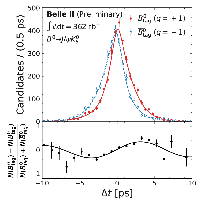
Refer to caption
Refer to caption
Figure 8: Background-subtracted ΔtΔ𝑡\Delta t distributions for B0J/ψKS0\mathit{{B}{}_{\mspace{-3.0mu}\scriptstyle{}}^{\mspace{-1.0mu}\scriptstyle{$0$}}}\to\mathit{{J\mspace{-2.0mu}/\mspace{-2.0mu}\psi}{}_{\mspace{-3.0mu}\scriptstyle{}}^{\mspace{-1.0mu}\scriptstyle{}}}\mathit{{K}{}_{\mspace{-3.0mu}\scriptstyle{\text{S}}}^{\mspace{-1.0mu}\scriptstyle{$0$}}} (top) and B0J/ψK0\mathit{{B}{}_{\mspace{-3.0mu}\scriptstyle{}}^{\mspace{-1.0mu}\scriptstyle{$0$}}}\to\mathit{{J\mspace{-2.0mu}/\mspace{-2.0mu}\psi}{}_{\mspace{-3.0mu}\scriptstyle{}}^{\mspace{-1.0mu}\scriptstyle{}}}\mathit{{K}{}_{\mspace{-3.0mu}\scriptstyle{}}^{\mspace{-1.0mu}\scriptstyle{*$0$}}} (bottom) in the full r𝑟r range (points) and the best-fit function (lines) for opposite- and like-flavor B\mathit{{B}{}_{\mspace{-3.0mu}\scriptstyle{}}^{\mspace{-1.0mu}\scriptstyle{}}} pairs and the corresponding asymmetries.

Table 1 lists the statistical and systematic uncertainties on εtagsubscript𝜀tag\varepsilon_{\text{tag}} for B0Dπ()+\mathit{{B}{}_{\mspace{-3.0mu}\scriptstyle{}}^{\mspace{-1.0mu}\scriptstyle{$0$}}}\to\mathit{{D}{}_{\mspace{-3.0mu}\scriptstyle{}}^{\mspace{-1.0mu}\scriptstyle{(*)-}}}\mathit{{\pi}{}_{\mspace{-3.0mu}\scriptstyle{}}^{\mspace{-1.0mu}\scriptstyle{+}}} and S𝑆S and C𝐶C for B0J/ψKS0\mathit{{B}{}_{\mspace{-3.0mu}\scriptstyle{}}^{\mspace{-1.0mu}\scriptstyle{$0$}}}\to\mathit{{J\mspace{-2.0mu}/\mspace{-2.0mu}\psi}{}_{\mspace{-3.0mu}\scriptstyle{}}^{\mspace{-1.0mu}\scriptstyle{}}}\mathit{{K}{}_{\mspace{-3.0mu}\scriptstyle{\text{S}}}^{\mspace{-1.0mu}\scriptstyle{$0$}}}. Statistical uncertainties are computed by bootstrapping [46], resampling the B0Dπ()+\mathit{{B}{}_{\mspace{-3.0mu}\scriptstyle{}}^{\mspace{-1.0mu}\scriptstyle{$0$}}}\to\mathit{{D}{}_{\mspace{-3.0mu}\scriptstyle{}}^{\mspace{-1.0mu}\scriptstyle{(*)-}}}\mathit{{\pi}{}_{\mspace{-3.0mu}\scriptstyle{}}^{\mspace{-1.0mu}\scriptstyle{+}}} and B0J/ψKS0\mathit{{B}{}_{\mspace{-3.0mu}\scriptstyle{}}^{\mspace{-1.0mu}\scriptstyle{$0$}}}\to\mathit{{J\mspace{-2.0mu}/\mspace{-2.0mu}\psi}{}_{\mspace{-3.0mu}\scriptstyle{}}^{\mspace{-1.0mu}\scriptstyle{}}}\mathit{{K}{}_{\mspace{-3.0mu}\scriptstyle{\text{S}}}^{\mspace{-1.0mu}\scriptstyle{$0$}}} data 1000 times each. The statistical uncertainties are larger than the sum in quadrature of all the individual systematic uncertainties.

Table 1: Systematic and statistical uncertainties on εtagsubscript𝜀tag\varepsilon_{\text{tag}} for B0Dπ()+\mathit{{B}{}_{\mspace{-3.0mu}\scriptstyle{}}^{\mspace{-1.0mu}\scriptstyle{$0$}}}\to\mathit{{D}{}_{\mspace{-3.0mu}\scriptstyle{}}^{\mspace{-1.0mu}\scriptstyle{(*)-}}}\mathit{{\pi}{}_{\mspace{-3.0mu}\scriptstyle{}}^{\mspace{-1.0mu}\scriptstyle{+}}} and, S𝑆S and C𝐶C for B0J/ψKS0\mathit{{B}{}_{\mspace{-3.0mu}\scriptstyle{}}^{\mspace{-1.0mu}\scriptstyle{$0$}}}\to\mathit{{J\mspace{-2.0mu}/\mspace{-2.0mu}\psi}{}_{\mspace{-3.0mu}\scriptstyle{}}^{\mspace{-1.0mu}\scriptstyle{}}}\mathit{{K}{}_{\mspace{-3.0mu}\scriptstyle{\text{S}}}^{\mspace{-1.0mu}\scriptstyle{$0$}}}.
Source εtagsubscript𝜀tag\varepsilon_{\text{tag}} [%] S𝑆S C𝐶C
Detector alignment 0.08 0.005 0.003
Interaction region 0.16 0.002 0.002
Beam energy 0.03 <0.001absent0.001<0.001 0.001
ΔEΔ𝐸\Delta E-fit background model 0.11 0.001 0.001
ΔEΔ𝐸\Delta E-fit signal model 0.08 0.003 0.006
sWeight background subtraction 0.24 0.001 0.001
Fixed resolution-function parameters 0.07 0.004 0.004
τ𝜏\tau and Δmd\Delta m_{\mathit{{d}{}_{\mspace{-3.0mu}\scriptstyle{}}^{\mspace{-1.0mu}\scriptstyle{}}}} 0.06 0.001 <0.001absent0.001<0.001
σΔtsubscript𝜎Δ𝑡\sigma_{\Delta t} binning 0.04 <0.001absent0.001<0.001 <0.001absent0.001<0.001
ΔtΔ𝑡\Delta t-fit bias 0.09 0.002 0.005
CP𝐶𝑃C\!P violation in Btag\mathit{{B}{}_{\mspace{-3.0mu}\scriptstyle{\text{tag}}}^{\mspace{-1.0mu}\scriptstyle{}}} decay 0.011 0.006
B0Dπ()+\mathit{{B}{}_{\mspace{-3.0mu}\scriptstyle{}}^{\mspace{-1.0mu}\scriptstyle{$0$}}}\to\mathit{{D}{}_{\mspace{-3.0mu}\scriptstyle{}}^{\mspace{-1.0mu}\scriptstyle{(*)-}}}\mathit{{\pi}{}_{\mspace{-3.0mu}\scriptstyle{}}^{\mspace{-1.0mu}\scriptstyle{+}}} sample size 0.004 0.007
Total systematic uncertainty 0.36 0.014 0.013
Statistical uncertainty 0.43 0.035 0.026

Uncertainties on the alignment of the tracking system of Belle II detector [47], the shape and location of the IR, and the ee+\mathit{{e}{}_{\mspace{-3.0mu}\scriptstyle{}}^{\mspace{-1.0mu}\scriptstyle{+}}}\mathit{{e}{}_{\mspace{-3.0mu}\scriptstyle{}}^{\mspace{-1.0mu}\scriptstyle{-}}} beam energy propagate to uncertainties on ΔtΔ𝑡\Delta t, resulting in potential changes to εtagsubscript𝜀tag\varepsilon_{\text{tag}}, S𝑆S, and C𝐶C. We determine εtagsubscript𝜀tag\varepsilon_{\text{tag}}, S𝑆S, and C𝐶C from simulated events reconstructed assuming four detector misalignment scenarios and take their changes, added in quadrature, as systematic uncertainties. Both the IR and beam energy are determined from ee+μμ+\mathit{{e}{}_{\mspace{-3.0mu}\scriptstyle{}}^{\mspace{-1.0mu}\scriptstyle{+}}}\mathit{{e}{}_{\mspace{-3.0mu}\scriptstyle{}}^{\mspace{-1.0mu}\scriptstyle{-}}}\to\mathit{{\mu}{}_{\mspace{-3.0mu}\scriptstyle{}}^{\mspace{-1.0mu}\scriptstyle{+}}}\mathit{{\mu}{}_{\mspace{-3.0mu}\scriptstyle{}}^{\mspace{-1.0mu}\scriptstyle{-}}} events in 30-minute intervals. We determine εtagsubscript𝜀tag\varepsilon_{\text{tag}}, S𝑆S, and C𝐶C with the parameters of the IR and beam energy varied by their uncertainties and take the shifts as systematic uncertainties.

Uncertainties on ΔEΔ𝐸\Delta E-fit component shapes propagate to uncertainties on the background-subtracted ΔtΔ𝑡\Delta t distributions, resulting in potential changes to εtagsubscript𝜀tag\varepsilon_{\text{tag}}, S𝑆S, and C𝐶C. We fit using various models and take any resulting shifts, added in quadrature, as systematic uncertainties. For the fit to B0Dπ()+\mathit{{B}{}_{\mspace{-3.0mu}\scriptstyle{}}^{\mspace{-1.0mu}\scriptstyle{$0$}}}\to\mathit{{D}{}_{\mspace{-3.0mu}\scriptstyle{}}^{\mspace{-1.0mu}\scriptstyle{(*)-}}}\mathit{{\pi}{}_{\mspace{-3.0mu}\scriptstyle{}}^{\mspace{-1.0mu}\scriptstyle{+}}} data, these models are inclusion of an additional Gaussian function to model a small peaking background from BB¯\mathit{{B}{}_{\mspace{-3.0mu}\scriptstyle{}}^{\mspace{-1.0mu}\scriptstyle{}}}\mathit{{\mkern 4.0mu\overline{\mkern-4.0mu{B}}}{}_{\mspace{-2.0mu}\scriptstyle{}}^{\mspace{0.0mu}\scriptstyle{}}} events, variation of the fixed ratio of BB¯\mathit{{B}{}_{\mspace{-3.0mu}\scriptstyle{}}^{\mspace{-1.0mu}\scriptstyle{}}}\mathit{{\mkern 4.0mu\overline{\mkern-4.0mu{B}}}{}_{\mspace{-2.0mu}\scriptstyle{}}^{\mspace{0.0mu}\scriptstyle{}}} events to B0Dπ()+\mathit{{B}{}_{\mspace{-3.0mu}\scriptstyle{}}^{\mspace{-1.0mu}\scriptstyle{$0$}}}\to\mathit{{D}{}_{\mspace{-3.0mu}\scriptstyle{}}^{\mspace{-1.0mu}\scriptstyle{(*)-}}}\mathit{{\pi}{}_{\mspace{-3.0mu}\scriptstyle{}}^{\mspace{-1.0mu}\scriptstyle{+}}} events by ±20%plus-or-minuspercent20\pm 20\%, and the freeing of the ratio of B0DK()+\mathit{{B}{}_{\mspace{-3.0mu}\scriptstyle{}}^{\mspace{-1.0mu}\scriptstyle{$0$}}}\to\mathit{{D}{}_{\mspace{-3.0mu}\scriptstyle{}}^{\mspace{-1.0mu}\scriptstyle{(*)-}}}\mathit{{K}{}_{\mspace{-3.0mu}\scriptstyle{}}^{\mspace{-1.0mu}\scriptstyle{+}}} to B0Dπ()+\mathit{{B}{}_{\mspace{-3.0mu}\scriptstyle{}}^{\mspace{-1.0mu}\scriptstyle{$0$}}}\to\mathit{{D}{}_{\mspace{-3.0mu}\scriptstyle{}}^{\mspace{-1.0mu}\scriptstyle{(*)-}}}\mathit{{\pi}{}_{\mspace{-3.0mu}\scriptstyle{}}^{\mspace{-1.0mu}\scriptstyle{+}}} events. Variations to the background models in the fits to B0J/ψKS0\mathit{{B}{}_{\mspace{-3.0mu}\scriptstyle{}}^{\mspace{-1.0mu}\scriptstyle{$0$}}}\to\mathit{{J\mspace{-2.0mu}/\mspace{-2.0mu}\psi}{}_{\mspace{-3.0mu}\scriptstyle{}}^{\mspace{-1.0mu}\scriptstyle{}}}\mathit{{K}{}_{\mspace{-3.0mu}\scriptstyle{\text{S}}}^{\mspace{-1.0mu}\scriptstyle{$0$}}} data have negligible impact. For the signal components, we varied fixed parameters within their uncertainties one by one.

The process of subtracting the backgrounds using sWeight is itself a source of uncertainty. For B0J/ψKS0\mathit{{B}{}_{\mspace{-3.0mu}\scriptstyle{}}^{\mspace{-1.0mu}\scriptstyle{$0$}}}\to\mathit{{J\mspace{-2.0mu}/\mspace{-2.0mu}\psi}{}_{\mspace{-3.0mu}\scriptstyle{}}^{\mspace{-1.0mu}\scriptstyle{}}}\mathit{{K}{}_{\mspace{-3.0mu}\scriptstyle{\text{S}}}^{\mspace{-1.0mu}\scriptstyle{$0$}}}, it is accounted for in the ΔtΔ𝑡\Delta t-fit bias discussed below. We account for the uncertainty in the background subtraction in B0Dπ()+\mathit{{B}{}_{\mspace{-3.0mu}\scriptstyle{}}^{\mspace{-1.0mu}\scriptstyle{$0$}}}\to\mathit{{D}{}_{\mspace{-3.0mu}\scriptstyle{}}^{\mspace{-1.0mu}\scriptstyle{(*)-}}}\mathit{{\pi}{}_{\mspace{-3.0mu}\scriptstyle{}}^{\mspace{-1.0mu}\scriptstyle{+}}} by determining εtagsubscript𝜀tag\varepsilon_{\text{tag}}, S𝑆S, and C𝐶C replacing the ΔtΔ𝑡\Delta t distributions with those from 1 ab1times1superscriptab11\text{\,}\mathrm{a}\mathrm{b}^{-1} of simulated B0Dπ()+\mathit{{B}{}_{\mspace{-3.0mu}\scriptstyle{}}^{\mspace{-1.0mu}\scriptstyle{$0$}}}\to\mathit{{D}{}_{\mspace{-3.0mu}\scriptstyle{}}^{\mspace{-1.0mu}\scriptstyle{(*)-}}}\mathit{{\pi}{}_{\mspace{-3.0mu}\scriptstyle{}}^{\mspace{-1.0mu}\scriptstyle{+}}} data that either contain signal events or signal and background events with background subtraction using sWeight, and take the differences as systematic uncertainties. This is the dominant systematic uncertainty on εtagsubscript𝜀tag\varepsilon_{\text{tag}}.

Uncertainties on ΔtΔ𝑡\Delta t-fit shape parameters directly propagate to changes to εtagsubscript𝜀tag\varepsilon_{\text{tag}}, S𝑆S, and C𝐶C. We repeat the fits with fixed resolution-function parameters freed one at a time and take the resulting changes to εtagsubscript𝜀tag\varepsilon_{\text{tag}}, S𝑆S, and C𝐶C, added in quadrature, as systematic uncertainties. We also repeat the fits with τ𝜏\tau and Δmd\Delta m_{\mathit{{d}{}_{\mspace{-3.0mu}\scriptstyle{}}^{\mspace{-1.0mu}\scriptstyle{}}}} varied within their known uncertainties [37] and take the resulting changes, added in quadrature, as systematic uncertainties. Finally, we repeat the fits with the numbers of bins for the σΔtsubscript𝜎Δ𝑡\sigma_{\Delta t} histogrammed probability density functions varied between 200 and 1000 and take the largest changes as systematic uncertainties.

The ΔtΔ𝑡\Delta t fits have biases that we determine from fits to simulated data sets equivalent in size to the real data, 20 such sets for B0Dπ()+\mathit{{B}{}_{\mspace{-3.0mu}\scriptstyle{}}^{\mspace{-1.0mu}\scriptstyle{$0$}}}\to\mathit{{D}{}_{\mspace{-3.0mu}\scriptstyle{}}^{\mspace{-1.0mu}\scriptstyle{(*)-}}}\mathit{{\pi}{}_{\mspace{-3.0mu}\scriptstyle{}}^{\mspace{-1.0mu}\scriptstyle{+}}} and 290 for B0J/ψKS0\mathit{{B}{}_{\mspace{-3.0mu}\scriptstyle{}}^{\mspace{-1.0mu}\scriptstyle{$0$}}}\to\mathit{{J\mspace{-2.0mu}/\mspace{-2.0mu}\psi}{}_{\mspace{-3.0mu}\scriptstyle{}}^{\mspace{-1.0mu}\scriptstyle{}}}\mathit{{K}{}_{\mspace{-3.0mu}\scriptstyle{\text{S}}}^{\mspace{-1.0mu}\scriptstyle{$0$}}}. We take the quadratic sum of the biases and their uncertainties as systematic uncertainties.

Equation (7) does not account for CP𝐶𝑃C\!P violation in Btag\mathit{{B}{}_{\mspace{-3.0mu}\scriptstyle{\text{tag}}}^{\mspace{-1.0mu}\scriptstyle{}}} decays [48]. This yields a systematic uncertainty determined in Ref. [3], which is the dominant systematic uncertainty on S𝑆S. We propagate the statistical uncertainties on GFlaT’s parameters and resolution-function parameters, arising from the B0Dπ()+\mathit{{B}{}_{\mspace{-3.0mu}\scriptstyle{}}^{\mspace{-1.0mu}\scriptstyle{$0$}}}\to\mathit{{D}{}_{\mspace{-3.0mu}\scriptstyle{}}^{\mspace{-1.0mu}\scriptstyle{(*)-}}}\mathit{{\pi}{}_{\mspace{-3.0mu}\scriptstyle{}}^{\mspace{-1.0mu}\scriptstyle{+}}} sample size, to uncertainties on S𝑆S and C𝐶C by repeating the fits for each B0Dπ()+\mathit{{B}{}_{\mspace{-3.0mu}\scriptstyle{}}^{\mspace{-1.0mu}\scriptstyle{$0$}}}\to\mathit{{D}{}_{\mspace{-3.0mu}\scriptstyle{}}^{\mspace{-1.0mu}\scriptstyle{(*)-}}}\mathit{{\pi}{}_{\mspace{-3.0mu}\scriptstyle{}}^{\mspace{-1.0mu}\scriptstyle{+}}} bootstrap sample.

VI Summary

We report on a new B\mathit{{B}{}_{\mspace{-3.0mu}\scriptstyle{}}^{\mspace{-1.0mu}\scriptstyle{}}} flavor tagger, GFlaT, for Belle II that uses a graph-neural-network to account for the correlated information among the decay products of the tag-side B\mathit{{B}{}_{\mspace{-3.0mu}\scriptstyle{}}^{\mspace{-1.0mu}\scriptstyle{}}}. We calibrate it using flavor-specific hadronic B\mathit{{B}{}_{\mspace{-3.0mu}\scriptstyle{}}^{\mspace{-1.0mu}\scriptstyle{}}} decays reconstructed in a 362±2 fb1timesuncertain3622superscriptfb1362\pm 2\text{\,}\mathrm{f}\mathrm{b}^{-1} sample of Belle II data and determine an effective tagging efficiency of

εtag=(37.40±0.43±0.36)%,subscript𝜀tagpercentplus-or-minus37.400.430.36\varepsilon_{\text{tag}}=(37.40\pm 0.43\pm 0.36)\%, (8)

where the first uncertainty is statistical and the second is systematic. For comparison, using the same data, we determine εtagsubscript𝜀tag\varepsilon_{\text{tag}} = 31.68±0.45 %timesuncertain31.680.45percent31.68\pm 0.45\text{\,}\mathrm{\char 37\relax} for the Belle II category-based flavor tagger.444Systematic uncertainties were not explicitly computed for the category-based flavor tagger, as they are expected to be very similar to and fully correlated with those from GFlaT. The GFlaT algorithm thus has an 18% better effective tagging efficiency.

We demonstrate GFlaT by measuring S𝑆S and C𝐶C for B0J/ψKS0\mathit{{B}{}_{\mspace{-3.0mu}\scriptstyle{}}^{\mspace{-1.0mu}\scriptstyle{$0$}}}\to\mathit{{J\mspace{-2.0mu}/\mspace{-2.0mu}\psi}{}_{\mspace{-3.0mu}\scriptstyle{}}^{\mspace{-1.0mu}\scriptstyle{}}}\mathit{{K}{}_{\mspace{-3.0mu}\scriptstyle{\text{S}}}^{\mspace{-1.0mu}\scriptstyle{$0$}}},

S𝑆\displaystyle S =\displaystyle=\leavevmode\nobreak\ 0.7240.724\displaystyle 0.724 ± 0.035plus-or-minus0.035\displaystyle\leavevmode\nobreak\ \pm\leavevmode\nobreak\ 0.035 ± 0.014,plus-or-minus0.014\displaystyle\leavevmode\nobreak\ \pm\leavevmode\nobreak\ 0.014, (9)
C𝐶\displaystyle C =\displaystyle=\leavevmode\nobreak\ 0.0350.035\displaystyle-0.035 ± 0.026plus-or-minus0.026\displaystyle\leavevmode\nobreak\ \pm\leavevmode\nobreak\ 0.026 ± 0.013,plus-or-minus0.013\displaystyle\leavevmode\nobreak\ \pm\leavevmode\nobreak\ 0.013, (10)

with a statistical correlation between S𝑆S and C𝐶C of 0.32, which agree with previous measurements [37, 2, 3, 4]. The statistical uncertainties are 8% and 7% smaller, respectively, than they would be if measured using the category-based flavor tagger, as expected given GFlaT’s higher effective tagging efficiency. From S𝑆S, we calculate ϕ1subscriptitalic-ϕ1\phi_{1} = 23.2±1.5 °timesuncertain23.21.5degree23.2\pm 1.5\text{\,}\mathrm{\SIUnitSymbolDegree}.555The other solution π/2ϕ1𝜋2subscriptitalic-ϕ1\pi/2-\phi_{1} is excluded from independent measurements [49]

Acknowledgements

This work, based on data collected using the Belle II detector, which was built and commissioned prior to March 2019, was supported by Higher Education and Science Committee of the Republic of Armenia Grant No. 23LCG-1C011; Australian Research Council and Research Grants No. DP200101792, No. DP210101900, No. DP210102831, No. DE220100462, No. LE210100098, and No. LE230100085; Austrian Federal Ministry of Education, Science and Research, Austrian Science Fund No. P 31361-N36 and No. J4625-N, and Horizon 2020 ERC Starting Grant No. 947006 “InterLeptons”; Natural Sciences and Engineering Research Council of Canada, Compute Canada and CANARIE; National Key R&D Program of China under Contract No. 2022YFA1601903, National Natural Science Foundation of China and Research Grants No. 11575017, No. 11761141009, No. 11705209, No. 11975076, No. 12135005, No. 12150004, No. 12161141008, and No. 12175041, and Shandong Provincial Natural Science Foundation Project ZR2022JQ02; the Czech Science Foundation Grant No. 22-18469S; European Research Council, Seventh Framework PIEF-GA-2013-622527, Horizon 2020 ERC-Advanced Grants No. 267104 and No. 884719, Horizon 2020 ERC-Consolidator Grant No. 819127, Horizon 2020 Marie Sklodowska-Curie Grant Agreement No. 700525 “NIOBE” and No. 101026516, and Horizon 2020 Marie Sklodowska-Curie RISE project JENNIFER2 Grant Agreement No. 822070 (European grants); L’Institut National de Physique Nucléaire et de Physique des Particules (IN2P3) du CNRS and L’Agence Nationale de la Recherche (ANR) under grant ANR-21-CE31-0009 (France); BMBF, DFG, HGF, MPG, and AvH Foundation (Germany); Department of Atomic Energy under Project Identification No. RTI 4002, Department of Science and Technology, and UPES SEED funding programs No. UPES/R&D-SEED-INFRA/17052023/01 and No. UPES/R&D-SOE/20062022/06 (India); Israel Science Foundation Grant No. 2476/17, U.S.-Israel Binational Science Foundation Grant No. 2016113, and Israel Ministry of Science Grant No. 3-16543; Istituto Nazionale di Fisica Nucleare and the Research Grants BELLE2; Japan Society for the Promotion of Science, Grant-in-Aid for Scientific Research Grants No. 16H03968, No. 16H03993, No. 16H06492, No. 16K05323, No. 17H01133, No. 17H05405, No. 18K03621, No. 18H03710, No. 18H05226, No. 19H00682, No. 20H05850, No. 20H05858, No. 22H00144, No. 22K14056, No. 22K21347, No. 23H05433, No. 26220706, and No. 26400255, the National Institute of Informatics, and Science Information NETwork 5 (SINET5), and the Ministry of Education, Culture, Sports, Science, and Technology (MEXT) of Japan; National Research Foundation (NRF) of Korea Grants No. 2016R1D1A1B02012900, No. 2018R1A2B3003643, No. 2018R1A6A1A06024970, No. 2019R1I1A3A01058933, No. 2021R1A6A1A03043957, No. 2021R1F1A1060423, No. 2021R1F1A1064008, No. 2022R1A2C1003993, and No. RS-2022-00197659, Radiation Science Research Institute, Foreign Large-Size Research Facility Application Supporting project, the Global Science Experimental Data Hub Center of the Korea Institute of Science and Technology Information and KREONET/GLORIAD; Universiti Malaya RU grant, Akademi Sains Malaysia, and Ministry of Education Malaysia; Frontiers of Science Program Contracts No. FOINS-296, No. CB-221329, No. CB-236394, No. CB-254409, and No. CB-180023, and SEP-CINVESTAV Research Grant No. 237 (Mexico); the Polish Ministry of Science and Higher Education and the National Science Center; the Ministry of Science and Higher Education of the Russian Federation and the HSE University Basic Research Program, Moscow; University of Tabuk Research Grants No. S-0256-1438 and No. S-0280-1439 (Saudi Arabia); Slovenian Research Agency and Research Grants No. J1-9124 and No. P1-0135; Agencia Estatal de Investigacion, Spain Grant No. RYC2020-029875-I and Generalitat Valenciana, Spain Grant No. CIDEGENT/2018/020; National Science and Technology Council, and Ministry of Education (Taiwan); Thailand Center of Excellence in Physics; TUBITAK ULAKBIM (Turkey); National Research Foundation of Ukraine, Project No. 2020.02/0257, and Ministry of Education and Science of Ukraine; the U.S. National Science Foundation and Research Grants No. PHY-1913789 and No. PHY-2111604, and the U.S. Department of Energy and Research Awards No. DE-AC06-76RLO1830, No. DE-SC0007983, No. DE-SC0009824, No. DE-SC0009973, No. DE-SC0010007, No. DE-SC0010073, No. DE-SC0010118, No. DE-SC0010504, No. DE-SC0011784, No. DE-SC0012704, No. DE-SC0019230, No. DE-SC0021274, No. DE-SC0021616, No. DE-SC0022350, No. DE-SC0023470; and the Vietnam Academy of Science and Technology (VAST) under Grants No. NVCC.05.12/22-23 and No. DL0000.02/24-25.

These acknowledgements are not to be interpreted as an endorsement of any statement made by any of our institutes, funding agencies, governments, or their representatives.

We thank the SuperKEKB team for delivering high-luminosity collisions; the KEK cryogenics group for the efficient operation of the detector solenoid magnet; the KEK computer group and the NII for on-site computing support and SINET6 network support; and the raw-data centers at BNL, DESY, GridKa, IN2P3, INFN, and the University of Victoria for off-site computing support.

Appendix A GFlaT parameters

Table 2 lists atagsubscript𝑎taga_{\text{tag}}, w¯¯𝑤\bar{w}, and ΔwΔ𝑤\Delta w for each r𝑟r bin, measured from events with B0Dπ()+\mathit{{B}{}_{\mspace{-3.0mu}\scriptstyle{}}^{\mspace{-1.0mu}\scriptstyle{$0$}}}\to\mathit{{D}{}_{\mspace{-3.0mu}\scriptstyle{}}^{\mspace{-1.0mu}\scriptstyle{(*)-}}}\mathit{{\pi}{}_{\mspace{-3.0mu}\scriptstyle{}}^{\mspace{-1.0mu}\scriptstyle{+}}}. The sources of systematic uncertainty are the same as listed in Table 1 for εtagsubscript𝜀tag\varepsilon_{\text{tag}}. Figure 9 shows the statistical correlation coefficients between the parameters that are used as inputs to estimate systematic uncertainties for S𝑆S and C𝐶C.

Table 2: GFlaT parameters in each r𝑟r bin.
r𝑟r bin atagsubscript𝑎taga_{\text{tag}} [%] w¯¯𝑤\bar{w} [%] ΔwΔ𝑤\Delta w [%]
[0.0,0.1]0.00.1[$0.0$,$0.1$] 1.72±1.47±1.32plus-or-minus1.721.471.32-1.72\pm 1.47\pm 1.32 48.29±0.78±0.75plus-or-minus48.290.780.7548.29\pm 0.78\pm 0.75 0.78±1.16±0.71plus-or-minus0.781.160.710.78\pm 1.16\pm 0.71
[0.1,0.25]0.10.25[$0.1$,$0.25$] 0.94±1.36±1.45plus-or-minus0.941.361.45-0.94\pm 1.36\pm 1.45 42.07±0.72±0.32plus-or-minus42.070.720.3242.07\pm 0.72\pm 0.32 1.41±1.06±0.92plus-or-minus1.411.060.92-1.41\pm 1.06\pm 0.92
[0.25,0.45]0.250.45[$0.25$,$0.45$] 0.28±1.28±1.46plus-or-minus0.281.281.46-0.28\pm 1.28\pm 1.46 34.63±0.61±0.61plus-or-minus34.630.610.6134.63\pm 0.61\pm 0.61 0.04±0.97±1.28plus-or-minus0.040.971.28-0.04\pm 0.97\pm 1.28
[0.45,0.6]0.450.6[$0.45$,$0.6$] 3.21±1.44±1.50plus-or-minus3.211.441.503.21\pm 1.44\pm 1.50 24.17±0.68±0.36plus-or-minus24.170.680.3624.17\pm 0.68\pm 0.36 1.64±1.13±0.52plus-or-minus1.641.130.521.64\pm 1.13\pm 0.52
[0.6,0.725]0.60.725[$0.6$,$0.725$] 1.17±1.58±1.47plus-or-minus1.171.581.471.17\pm 1.58\pm 1.47 16.98±0.68±0.92plus-or-minus16.980.680.9216.98\pm 0.68\pm 0.92 1.36±1.15±0.72plus-or-minus1.361.150.721.36\pm 1.15\pm 0.72
[0.725,0.875]0.7250.875[$0.725$,$0.875$] 1.13±1.30±1.55plus-or-minus1.131.301.55-1.13\pm 1.30\pm 1.55 11.50±0.53±0.39plus-or-minus11.500.530.3911.50\pm 0.53\pm 0.39 0.26±0.92±0.71plus-or-minus0.260.920.71-0.26\pm 0.92\pm 0.71
[0.875,1.0]0.8751.0[$0.875$,$1.0$] 0.18±0.91±1.30plus-or-minus0.180.911.30-0.18\pm 0.91\pm 1.30 2.62±0.27±0.14plus-or-minus2.620.270.142.62\pm 0.27\pm 0.14 0.75±0.53±0.60plus-or-minus0.750.530.600.75\pm 0.53\pm 0.60
Refer to caption
Figure 9: Correlation coefficients, in 102superscript10210^{-2}, between the GFlaT parameters. Subscripts indicate r𝑟r bins.

References