RIME: Robust Preference-based Reinforcement Learning with Noisy Preferences

Abstract

Preference-based Reinforcement Learning (PbRL) avoids the need for reward engineering by harnessing human preferences as the reward signal. However, current PbRL algorithms over-reliance on high-quality feedback from domain experts, which results in a lack of robustness. In this paper, we present RIME, a robust PbRL algorithm for effective reward learning from noisy preferences. Our method incorporates a sample selection-based discriminator to dynamically filter denoised preferences for robust training. To mitigate the accumulated error caused by incorrect selection, we propose to warm start the reward model, which additionally bridges the performance gap during transition from pre-training to online training in PbRL. Our experiments on robotic manipulation and locomotion tasks demonstrate that RIME significantly enhances the robustness of the current state-of-the-art PbRL method. Ablation studies further demonstrate that the warm start is crucial for both robustness and feedback-efficiency in limited-feedback cases.

1 Introduction

Reinforcement Learning (RL) has demonstrated remarkable performance in various domains, including gameplay (Vinyals et al., 2019; Perolat et al., 2022; Kaufmann et al., 2023), robotics (Chen et al., 2022), autonomous systems (Bellemare et al., 2020; Zhou et al., 2020), etc. However, the key determinant of RL success often hinges on the careful design of reward functions, which can be both labor-intensive and error-prone. In this context, Preference-Based RL (PbRL) (Akrour et al., 2011; Christiano et al., 2017) emerges as a valuable alternative, negating the need for hand-crafted reward functions. PbRL adopts a human-in-the-loop paradigm, where human teachers provide preferences over distinct agent behaviors as the reward signal.

Nevertheless, existing works in PbRL have primarily focused on enhancing feedback-efficiency, aiming to maximize the expected cumulative rewards with few number of feedback queries. This focus induces a substantial reliance on high-quality feedback, typically assuming expertise on the teachers (Liu et al., 2022; Kim et al., 2022). However, humans are prone to errors (Christiano et al., 2017). In broader applications, feedback is often sourced from non-expert users or crowd-sourcing platforms, where the quality can be inconsistent and noisy. Further complicating the matter, Lee et al. (2021a) showed that even a mere 10% corruption rate in preference labels can dramatically degrade the performance. The lack of robustness to noisy preference labels hinders the wide application of PbRL.

Meanwhile, learning from noisy labels, also known as robust training, is a rising concern in deep learning, as such labels severely degrade the generalization performance of deep neural networks. Song et al. (2022) classifies robust training methods into four key categories: robust architecture (Cheng et al., 2020), robust regularization (Xia et al., 2020), robust loss design (Lyu & Tsang, 2019), and sample selection (Li et al., 2020; Song et al., 2021). However, it poses challenges to incorporate these advanced methods for robust training in PbRL. This complexity arises due to the limited number of feedback, which is often restricted to only hundreds of feedback in some tasks for the sake of feedback-efficiency and cost reduction, as well as the potential distribution shift issue during RL training.

Figure 1: Overview of RIME. In the pre-training phase, we warm start the reward model $\hat{r}_{\psi}$ with intrinsic rewards $r^{\text{int}}$ to facilitate a smooth transition to online training phase. Post pre-training, the policy, Q-network, and reward model $\hat{r}_{\psi}$ are all inherited as initial configurations for online training. During online training, we utilize a denoising discriminator to screen denoised preferences for robust reward learning. This discriminator employs a dynamic lower bound $\tau_{\text{lower}}$ on the KL divergence between predicted preferences $P_{\psi}$ and annotated preference labels $\tilde{y}$ to filter trustworthy samples $\mathcal{D}_{t}$, and an upper bound $\tau_{\text{upper}}$ to flip highly unreliable labels $\mathcal{D}_{f}$.

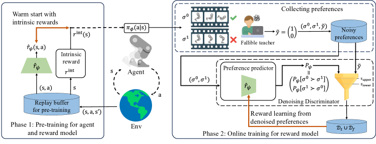
In this work, we aim to improve the robustness of preference-based RL methods on noisy and quantitatively limited preferences. To this end, we present RIME: Robust preference-based reInforcement learning via warM-start dEnoising discriminator. RIME modifies the training paradigm of the reward model in widely-adopted two-phase (i.e.pre-training and online training phases) pipeline of PbRL. Figure 1 shows an overview of RIME. In particular, to empower robust learning from noisy preferences, we introduce a denoising discriminator. It utilizes dynamic lower and predefined upper bounds on the Kullback–Leibler (KL) divergence between predicted and annotated preference labels to filter samples. Further, to mitigate the accumulated error caused by incorrect filtration, we propose to warm start the reward model during the pre-training phase for a good initialization. Moreover, we find that the warm start also bridges the performance gap that occurs during the transition from pre-training to online training. Our experiments demonstrate that RIME exceeds existing baselines by a large margin in noisy conditions and considerably improves robustness.

In summary, our work has three main contributions. First, we present RIME, a robust reward learning algorithm for PbRL, designed to effectively train reward models from noisy feedback—an important and realistic topic that has not been studied extensively. Second, we observe a dramatic performance gap during the transition from pre-training to online training in PbRL, and propose to warm start the reward model for seamless transition, which proves to be crucial for both robustness and feedback-efficiency in limited-feedback cases. Last, we show that RIME outperforms existing PbRL baselines under noisy feedback settings, across a diverse set of robotic manipulation tasks from Meta-World (Yu et al., 2020) and locomotion tasks from the DeepMind Control Suite (Tassa et al., 2018, 2020), and further is more suitable for non-expert humans.

2 Related work

Preference-based Reinforcement Learning. Incorporating human feedback into the training of reward models has proven effective in various domains, including natural language processing (Ouyang et al., 2022), multi-modal (Lee et al., 2023), and reinforcement learning (Christiano et al., 2017; Ibarz et al., 2018; Hejna III & Sadigh, 2023). In the context of RL, Christiano et al. (2017) proposed a comprehensive framework for PbRL. To improve feedback-efficiency, PEBBLE (Lee et al., 2021b) used unsupervised exploration for policy pre-training. SURF (Park et al., 2021) employed data augmentation and semi-supervised learning to enrich the preference dataset. RUNE (Liang et al., 2021) encouraged exploration by modulating reward uncertainty. MRN (Liu et al., 2022) introduced a bi-level optimization to optimize the Q-function’s performance. PT (Kim et al., 2022) utilized Transformer architecture to model non-Markovian rewards, proving effective in complex tasks.

Despite these advancements, the focus on feedback efficiency should not overshadow the equally critical issue of robustness in PbRL. Lee et al. (2021a) indicated that a mere 10% rate of corrupted preference labels can significantly impair algorithmic performance. Moreover, in broader application scenarios, the gathering of non-expert preferences exacerbates the risk of introducing erroneous labels. Therefore, enhancing the robustness in PbRL remains a vital research direction. In this work, we address robust PbRL via a warm-start denoising discriminator, which dynamically filter denoised preferences and is more adaptable to distribution shift cases during RL training.

Learning from Noisy Labels. Learning from noisy labels has gained more attention in supervised learning, particularly in light of the widespread presence of noisy or imprecise labels in real-world applications. A variety of approaches have been proposed for robust training (Song et al., 2022), including architectural modifications (Goldberger & Ben-Reuven, 2016), regularization (Lukasik et al., 2020), loss function designs (Zhang & Sabuncu, 2018), and sample selection methods (Wang et al., 2021). Despite these advancements, the direct application of these methods to reward learning in PbRL has presented challenges, notably due to the limited sample sizes and the absence of i.i.d. of samples. In PbRL, Xue et al. (2023) proposed an encoder-decoder architecture to model diverse human preferences, which required approximate 100 times amount of preference labels used in our experiments. Our approach can be situated within the sample selection category and improves robustness while preserving feedback-efficiency.

Policy-to-Value Reincarnating RL. Policy-to-value reincarnating RL (PVRL) represents transferring a sub-optimal teacher policy to a value-based RL student agent (Agarwal et al., 2022). Uchendu et al. (2023) found that a randomly initialized Q-network in PVRL leads to the teacher policy being forgotten quickly. Within the widely-adopted pipeline of PbRL, the challenge intrinsic to PVRL also arise during the transition from pre-training to online training, but has been neglected in previous research (Lee et al., 2021b; Park et al., 2021; Liang et al., 2021; Liu et al., 2022). The issue of forgetting pre-training policy becomes more critical under noisy feedback conditions. Based on the observation, we propose to warm start the reward model for a seamless transition. Our ablation study demonstrates that the warm start is crucial for both robustness and feedback-efficiency.

3 Preliminaries

Preference-based Reinforcement Learning. In standard RL, an agent interacts with an environment in discrete time steps (Sutton & Barto, 2018). At each time step $t$, the agent observes the current state $\mathbf{s}_{t}$ and selects an action $\mathbf{a}_{t}$ according to its policy $\pi(\mathbf{a}_{t}|\mathbf{s}_{t})$. The environment responds by emitting a reward $r(\mathbf{s}_{t},\mathbf{a}_{t})$ and transitioning to the next state $\mathbf{s}_{t+1}$. The agent’s objective is to learn a policy that maximizes the expected return.

In Preference-based RL, there is no predefined reward function. Instead, a teacher offers preferences between agent’s behaviors and an estimated reward function $\hat{r}_{\psi}$ is trained to align with collected preferences. Following previous works (Lee et al., 2021b; Liu et al., 2022; Kim et al., 2022), we consider preferences over two trajectory segments of length $H$, where segment $\sigma=\{(\mathbf{s}_{1},\mathbf{a}_{1}),...,(\mathbf{s}_{H},\mathbf{a}_{H})\}$. Given a pair of segments $(\sigma^{0},\sigma^{1})$, a teacher provides a preference label $\tilde{y}$ from the set $\{(1,0),(0,1),(0.5,0.5)\}$. The label $\tilde{y}=(1,0)$ signifies $\sigma^{0}\succ\sigma^{1}$, $\tilde{y}=(0,1)$ signifies $\sigma^{1}\succ\sigma^{0}$, and $\tilde{y}=(0.5,0.5)$ represents an equally preferable case, where $\sigma^{i}\succ\sigma^{j}$ denotes that segment $i$ is preferred over segment $j$. Each feedback is stored in a dataset $\mathcal{D}$ as a triple $(\sigma^{0},\sigma^{1},\tilde{y})$. Following the Bradley-Terry model (Bradley & Terry, 1952), the preference predicted by the estimated reward function $\hat{r}_{\psi}$ is formulated as:

$$P_{\psi}[\sigma^{i}\succ\sigma^{j}]=\frac{\exp\left(\sum_{t}\hat{r}_{\psi}(\mathbf{s}^{i}_{t},\mathbf{a}^{i}_{t})\right)}{\sum_{k=i,j}\exp\left(\sum_{t}\hat{r}_{\psi}(\mathbf{s}^{k}_{t},\mathbf{a}^{k}_{t})\right)}$$ (1)

The estimated reward function $\hat{r}_{\psi}$ is updated by minimizing the cross-entropy loss between the predicted preferences $P_{\psi}$ and the annotated labels $\tilde{y}$:

$$\mathcal{L}^{\mathtt{CE}}(\psi)=\operatorname*{\mathbb{E}}\Big{[}\mathcal{L}^{\mathtt{Reward}}\Big{]}=-\operatorname*{\mathbb{E}} \Big{[}\tilde{y}(0)\ln P_{\psi}[\sigma^{0}\succ\sigma^{1}]$$

$$+ \tilde{y}(1)\ln P_{\psi}[\sigma^{1}\succ\sigma^{0}]\Big{]}$$ (2)

The policy $\pi$ can subsequently be updated using any RL algorithm to maximize the expected return with respect to the estimated reward function $\hat{r}_{\psi}$.

Unsupervised Pre-training in PbRL. Pre-training agents is important in PbRL because the initial random policy often results in uninstructive preference queries, requiring lots of queries for even elementary learning progress. Recent study addressed this issue through unsupervised exploration for policy pre-training (Lee et al., 2021b). Specifically, agents are encouraged to traverse a more expansive state space by utilizing an intrinsic reward function derived from particle-based state entropy (Singh et al., 2003). Formally, the intrinsic reward is defined as (Liu & Abbeel, 2021):

$$r^{\text{int}}(\mathbf{s}_{t})=\log(\lVert\mathbf{s}_{t}-\mathbf{s}_{t}^{k}\rVert)$$ (3)

where $\mathbf{s}_{t}^{k}$ is the $k$-th nearest neighbor of $\mathbf{s}_{t}$. This reward motivates the agent to explore a broader diversity of states. This exploration, in turn, leads to a varied set of agent’s behaviors, facilitating more informative preference queries.

Noisy Preferences in PbRL. We denote the annotated preference labels as $\tilde{y}$ and the ground-truth preference labels, typically sourced from expert human teachers or scripted teachers, as $y$. To simulate the noise in human annotations, Lee et al. (2021a) introduced four noisy 0-1 labeling models: Equal, Skip, Myopic, and Mistake. The “Mistake” model, in particular, proved to be significantly detrimental to performance across various environments. It hypothesizes that the preference dataset is contaminated with corrupted preferences whose annotated labels $\tilde{y}$ are $1-y$. Building upon these insights, our work starts from addressing robust reward learning under the mistake model settings because of the guidance that solutions designed for complex challenges could be effectively adapted to address simpler ones.

4 Method

In this section, we formally introduce RIME: Robust preference-based reInforcement learning via warM-start dEnoising discriminator. RIME consists two main components: 1) a denoising discriminator designed to filter out corrupted preference data while accounting for training instability and distribution shift issue, and 2) a warm start method to effectively initialize the reward model and enable a seamless transition from pre-training to online training. See Figure 1 for the overview of RIME. The full procedure of RIME is detailed in Appendix A.

4.1 Denoising Discriminator

In the presence of noisy labels, it is well motivated to distinguish between clean and corrupted samples for robust training. Existing research indicates that deep neural networks first learn generalizable patterns before overfitting to the noise in the data. Therefore, prioritizing samples associated with smaller losses as clean ones is a well-founded approach to improve robustness. Inspired by this insight, we theoretically establish a lower bound on the KL divergence between the predicted preference $P_{\psi}$ and the annotated preference $\tilde{y}$ for corrupted samples, in order to filter out large-loss corrupted samples.

Theorem 4.1 (KL Divergence Lower Bound for Corrupted Samples).

Consider a preference dataset $\{(\sigma^{0}_{i},\sigma^{1}_{i},\tilde{y}_{i})\}_{i=1}^{n}$, where $\tilde{y}_{i}$ is the annotated label for the segment pair $(\sigma^{0}_{i},\sigma^{1}_{i})$ with the ground truth label $y_{i}$. Let $x_{i}$ denote the tuple $(\sigma^{0}_{i},\sigma^{1}_{i})$. Assume the cross-entropy loss $\mathcal{L}^{\mathtt{CE}}$ for clean data (whose $\tilde{y}_{i}=y_{i}$) is bounded by $\rho$. Then, the KL divergence between the predicted preference $P_{\psi}(x)$ and the annotated label $\tilde{y}(x)$ for a corrupted sample $x$ is lower-bounded as:

$$D_{\mathrm{KL}}\left(P_{\psi}(x)\|\tilde{y}(x)\right)\geq-\ln\rho+\frac{\rho}{2}+\mathcal{O}(\rho^{2})$$ (4)

The proof of Theorem 4 is presented in Appendix C. Based on Theorem 4, we formulate the lower bound on KL divergence threshold to filter out untrustworthy samples as $\tau_{\text{base}}=-\ln\rho+\alpha\rho$ in practical, where $\rho$ denotes the maximum cross-entropy loss on trustworthy samples observed during the last update, and $\alpha$ serves as a tunable hyperparameter with a value range in $(0,0.5]$ in theoretical.

However, the shifting state distribution complicates the robust training problem in RL, compared to deep learning contexts. To add tolerance for trustworthy samples in cases of distribution shift, we introduce an auxiliary term characterizing the uncertainty for filtration, defined as $\tau_{\text{unc}}=\beta_{t}\cdot s_{\text{KL}}$, where $\beta_{t}$ is a time-dependent parameter, and $s_{\text{KL}}$ is the standard deviation of the KL divergence. Our intuition is that the inclusion of out-of-distribution data for training is likely to induce fluctuations in the training loss. Therefore, the complete threshold equation is formulated as follows:

$$\tau_{\text{lower}}=\tau_{\text{base}}+\tau_{\text{unc}}=-\ln\rho+\alpha\rho+\beta_{t}\cdot s_{\text{KL}}$$ (5)

We utilize a linear decay schedule for $\beta_{t}$ to initially allow greater tolerance for samples while becoming increasingly conservative over time, i.e.$\beta_{t}=\max(\beta_{\min},\beta_{\max}-kt)$. At each training step for the reward model, we apply the threshold in Equation (5) to identify trustworthy sample dataset $\mathcal{D}_{t}$, as described below:

$$\mathcal{D}_{t}=\{(\sigma^{0},\sigma^{1},\tilde{y})\,|\,D_{\mathrm{KL}}(P_{\psi}(\sigma^{0},\sigma^{1})\|\tilde{y})<\tau_{\text{lower}}\}$$ (6)

To ensure efficient usage of samples, we introduce a label-flipping method for the reintegration of untrustworthy samples. Specifically, we pre-define an upper bound $\tau_{\text{upper}}$ and reverse the labels for samples exceeding this threshold:

(7)

Beyond improving sample utilization, the label-flipping method also bolsters the model’s predictive confidence and reduce output entropy (Grandvalet & Bengio, 2004). Following two filtering steps, the reward model is trained on the unified datasets $\mathcal{D}_{t}\cup\mathcal{D}_{f}$, using the loss function as follows:

$$\mathcal{L}^{\mathtt{CE}}= \operatorname*{\mathbb{E}}_{(\sigma^{0},\sigma^{1},\tilde{y})\sim\mathcal{D}_{t}}\left[\mathcal{L}^{\mathtt{Reward}}(\sigma^{0},\sigma^{1},\tilde{y})\right]+$$

$$\operatorname*{\mathbb{E}}_{(\sigma^{0},\sigma^{1},1-\tilde{y})\sim\mathcal{D}_{f}}\left[\mathcal{L}^{\mathtt{Reward}}(\sigma^{0},\sigma^{1},1-\tilde{y})\right]$$ (8)

Our denoising discriminator belongs to the category of sample selection methods for robust training. However, it is different in using a dynamically adjusted threshold, augmented by a term that captures distributional shifts, making it more suitable for RL training process.

(a) $\epsilon=0.1$

(b) $\epsilon=0.15$

(c) $\epsilon=0.2$

(d) $\epsilon=0.25$

(e) $\epsilon=0.3$

Figure 2: Learning curves for robotic manipulation tasks from Meta-world, where each row represents a specific task and each column corresponds to a different error rate $\epsilon$. SAC serves as a performance upper bound, using a ground-truth reward function unavailable in PbRL settings. The corresponding number of feedback in total and per session are show in Table 1. The solid line and shaded regions respectively denote mean and standard deviation of success rate, across ten runs.

4.2 Warm Start

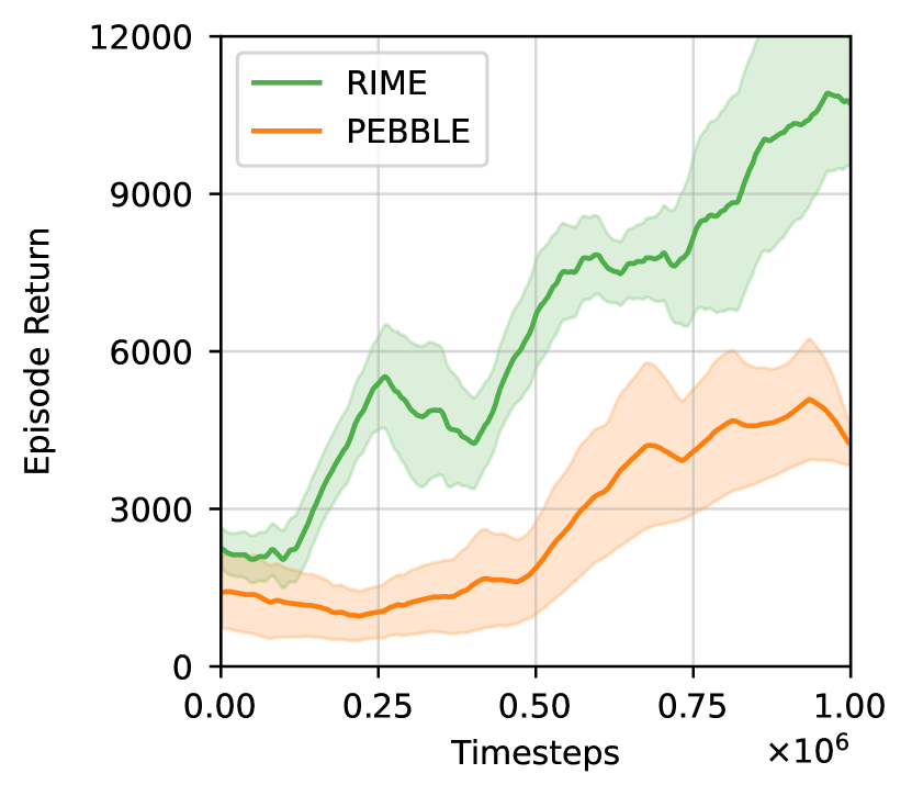
Sample selection methods frequently suffer from accumulated error due to incorrect selection, which underscores the need of good initialization for the discriminator to effectively differentiate between samples at initial. Meanwhile, we observe a marked degradation of performance during transition from pre-training to online training (see Figure 3). This gap is clearly observed under noisy feedback settings and is fatal to robustness. It is exacerbated when following the most widely-adopted backbone algorithm, PEBBLE, which resets the Q-network and only retains the pre-trained policy after the pre-training phase. The issue arises because the biased reward model, trained on noisy preferences, biasedly optimize the Q-network through minimizing Bellman residual. This, in turn, offers a poor learning signal for the policy, erasing any gains made during pre-training.

Figure 3: Performance degradation during transition on Walker-walk (left) and Quadruped-walk (right) with 30% noisy preferences. We pre-train an agent using SAC for 20k steps. Warm start method shows smaller transition gap and faster recovery.

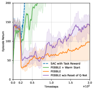
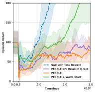
Inspired by these observations, we propose to warm start the reward model to facilitate a smoother transition from pre-training to online training. Specifically, we pre-train the reward model to approximate intrinsic rewards during pre-training phase. Because the output layer of the reward model typically uses the tanh activation function (Lee et al., 2021b), we firstly normalize the intrinsic reward to the range $(-1,1)$ as follows:

$$r^{\text{int}}_{\text{norm}}(\mathbf{s}_{t})=\text{clip}(\frac{r^{\text{int}}(\mathbf{s}_{t})-\bar{r}}{3\sigma_{r}},-1+\delta,1-\delta)$$ (9)

where $0<\delta\ll 1$. $\bar{r}$ and $\sigma_{r}$ are mean and standard deviation of the intrinsic rewards, respectively. Then the agent receives the reward $r^{\text{int}}_{\text{norm}}$ and stores each tuple $(\mathbf{s}_{t},\mathbf{a}_{t},r^{\text{int}}_{\text{norm}},\mathbf{s}_{t+1})$ in a replay buffer, denoted as $\mathcal{D}_{\text{pretrain}}$. During the reward model update, we sample batches of $(\mathbf{s}_{t},\mathbf{a}_{t})$ along with all encountered states $\mathcal{S}=\{\mathbf{s}|\mathbf{s}\text{ in }\mathcal{D}_{\text{pretrain}}\}$ for nearest neighbor searches. The loss function for updating the reward model $\hat{r}_{\psi}$ is given by the mean squared error as:

$$\mathcal{L}^{\mathtt{MSE}}=\operatorname*{\mathbb{E}}_{(\mathbf{s}_{t},\mathbf{a}_{t})\sim\mathcal{D}_{\text{pretrain}}}\Big{[}\frac{1}{2}\left(\hat{r}_{\psi}(\mathbf{s}_{t},\mathbf{a}_{t})-r^{\text{int}}_{\text{norm}}(\mathbf{s}_{t})\right)^{2}\Big{]}$$ (10)

Attributed to warm start, both the Q-network and reward model are aligned with intrinsic rewards, allowing for the retention of all knowledge gained during pre-training (i.e.policy, Q-network, and reward model) for subsequent online training. Moreover, the warm-started reward model contains more information than random initialization, enhancing the discriminator’s ability at initial.

5 Experiments

(a) $\epsilon=0.1$

(b) $\epsilon=0.15$

(c) $\epsilon=0.2$

(d) $\epsilon=0.25$

(e) $\epsilon=0.3$

Figure 4: Learning curves on locomotion tasks from DMControl, where each row represents a specific task and each column corresponds to a different error rate $\epsilon$ setting. SAC serves as a performance upper bound, using a ground-truth reward function unavailable in PbRL settings. The corresponding number of feedback in total and per session are show in Table 1. The solid line and shaded regions respectively denote mean and standard deviation of episode return, across ten runs.

5.1 Setups

We evaluate RIME on six complex tasks, including robotic manipulation tasks from Meta-world (Yu et al., 2020) and locomotion tasks from DMControl (Tassa et al., 2018, 2020). The details of experimental tasks are shown in Appendix D.1. Similar to prior works (Lee et al., 2021a, b; Park et al., 2021), to ensure a systematic and fair evaluation, we consider a scripted teacher that provides preferences between two trajectory segments based on the sum of ground-truth reward values for each segment. To generate noisy preferences, we follow the procedure of the “mistake” scripted teacher in Lee et al. (2021a), which flips correct preferences with a probability of $\epsilon$. We refer to $\epsilon$ as the error rate. We choose PEBBLE (Lee et al., 2021b) as our backbone algorithm to implement RIME. In our experiments, we compare RIME against ground-truth reward-based SAC and four state-of-the-art PbRL algorithms: PEBBLE (Lee et al., 2021b), SURF (Park et al., 2021), RUNE (Liang et al., 2021), and MRN (Liu et al., 2022). Here, SAC is considered as an upper bound for performance, as it utilizes a ground-truth reward function not available in PbRL settings. We include SAC in our comparisons because it is the backbone RL algorithm of PEBBLE.

Implementation Details. For the hyperparameters of RIME, we fix $\alpha=0.5$, $\beta_{\min}=1$ and $\beta_{\max}=3$ in the lower bound $\tau_{\text{lower}}$, and fix the upper bound $\tau_{\text{upper}}=3\ln(10)$ for all experiments. The decay rate $k$ in $\tau_{\text{upper}}$ is $1/30$ for DMControl tasks, and $1/300$ for Meta-world tasks, respectively. Other hyperparameters are kept the same with PEBBLE. For the sampling of queries, we use the disagreement sampling scheme for all PbRL algorithms, following the setting in Christiano et al. (2017). For the implementation of baselines, we use their corresponding publicly released repositories (see Table 6 for source codes). The feedback amount in total and per query session in each environment with specified error rate are detailed in Table 1.

For each task, we run all algorithms independently for ten times and report the average performance along with the standard deviation. Tasks from Meta-world are measured on success rate, while tasks from DMControl are measured on ground-truth episode return. More details on the algorithm implementation are provided in Appendix D.2.

Table 1: Feedback amount in each environment with specified error rate. Value column refers to feedback amount in total / per session.

Environment	Error rate	Value	Environment	Error rate	Value
Walker	$\epsilon<0.2$	$500/50$	Button Press	$\epsilon<0.2$	$10000/50$
Walker	$\epsilon\geq 0.2$	$1000/100$	Button Press	$\epsilon\geq 0.2$	$20000/100$
Cheetah	$\epsilon<0.2$	$500/50$	Sweep Into	$\epsilon<0.2$	$10000/50$
Cheetah	$\epsilon\geq 0.2$	$1000/100$	Sweep Into	$\epsilon\geq 0.2$	$20000/100$
Quadruped	$\epsilon<0.2$	$2000/200$	Hammer	$\epsilon<0.2$	$20000/100$
Quadruped	$\epsilon\geq 0.2$	$4000/400$	Hammer	$\epsilon=0.2,0.25$	$40000/200$
			Hammer	$\epsilon=0.3$	$80000/400$

5.2 Results

Table 2: Results on tasks from Meta-world and DMControl with “mistake” teacher. The result shows the mean and standard deviation of metric (i.e.episode return for DMControl tasks and success rate for Meta-world tasks) across all five error rates within 10 runs.

Algorithm	DMControl			Meta-world
	Walker	Cheetah	Quadruped	Button Press	Sweep Into	Hammer
PEBBLE	692.05 $\pm$ 192.67	604.77 $\pm$ 126.63	208.66 $\pm$ 106.81	50.07 $\pm$ 29.53	19.09 $\pm$ 29.82	26.22 $\pm$ 32.08
SURF	211.28 $\pm$ 195.25	341.43 $\pm$ 178.10	125.51 $\pm$ 040.15	42.60 $\pm$ 27.55	16.04 $\pm$ 22.86	11.43 $\pm$ 22.76
RUNE	584.06 $\pm$ 271.84	424.17 $\pm$ 205.16	152.66 $\pm$ 131.43	27.04 $\pm$ 18.89	15.02 $\pm$ 19.18	12.14 $\pm$ 19.30
MRN	537.40 $\pm$ 281.36	538.74 $\pm$ 169.63	139.65 $\pm$ 088.24	43.48 $\pm$ 30.58	14.74 $\pm$ 22.89	06.35 $\pm$ 09.55
RIME	837.79 $\pm$ 133.49	602.18 $\pm$ 096.10	415.52 $\pm$ 180.74	85.70 $\pm$ 22.92	51.96 $\pm$ 42.90	42.28 $\pm$ 42.31

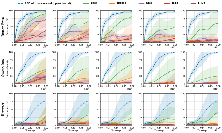
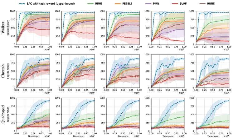
For robotic manipulation tasks, we consider three tasks from Meta-world: Button-press, Sweep-into, and Hammer. For locomotion tasks, we choose three environments from DMControl: Walker-walk, Cheetah-run, and Quadrupted-walk. Figure 2 and Figure 4 show the learning curves of RIME and baselines on Meta-world and DMControl tasks with five error rates, respectively. Table 2 shows the mean and standard deviation of metrics across the five error rates.

Since some preferences are corrupted, we observe that there is a gap between all PbRL methods and the best performance (i.e.SAC with task reward), but RIME exceeds the PbRL baselines by a large margin in almost all environments. Especially, RIME remains effective in cases where all baselines struggle, such as Button-press with $\epsilon=0.2$, Hammer with $\epsilon=0.3$ and Walker with $\epsilon=0.3$, etc. These results demonstrate that RIME significantly improves robustness against noisy preferences. We also observe that although some feedback-efficient baselines based on PEBBLE perform comparable or even exceed PEBBLE in low-level noise, they become ineffective as error rates rise. Additionally, Table 2 shows that PEBBLE is a robust algorithm second only to RIME. This reveals that the pursuit of feedback efficiency leads to over-reliance on feedback quality.

5.3 Ablation Study

Table 3: Results on tasks from Meta-world and DMControl with 4 other types of (noisy) teacher. The result shows the mean and standard deviation of metric (i.e.episode return for DMControl tasks and success rate for Meta-world tasks) averaged over 5 runs.

Domain	Environment	Algorithm	Oracle	Equal	Skip	Myopic	Average
DMControl	Walker	PEBBLE	877.44 $\pm$ 44.06	930.90 $\pm$ 17.77	904.31 $\pm$ 26.59	762.53 $\pm$ 165.98	868.80
		MRN	913.66 $\pm$ 51.84	942.80 $\pm$ 14.14	919.61 $\pm$ 48.87	882.34 $\pm$ 019.68	914.60
		RIME	958.87 $\pm$ 03.08	954.89 $\pm$ 01.43	950.83 $\pm$ 16.44	952.16 $\pm$ 001.80	954.19
	Quadruped	PEBBLE	620.35 $\pm$ 193.74	743.04 $\pm$ 107.30	776.01 $\pm$ 065.86	622.78 $\pm$ 200.04	690.55
		MRN	682.98 $\pm$ 182.25	666.56 $\pm$ 298.40	653.28 $\pm$ 150.78	525.91 $\pm$ 233.77	633.18
		RIME	678.36 $\pm$ 033.02	784.05 $\pm$ 056.96	755.58 $\pm$ 116.24	688.44 $\pm$ 130.59	726.61
Meta-world	Button-Press	PEBBLE	100.0 $\pm$ 0.0	100.0 $\pm$ 0.0	100.0 $\pm$ 0.0	099.8 $\pm$ 0.4	99.95
		MRN	100.0 $\pm$ 0.0	100.0 $\pm$ 0.0	099.6 $\pm$ 0.5	100.0 $\pm$ 0.0	99.90
		RIME	100.0 $\pm$ 0.0	100.0 $\pm$ 0.0	100.0 $\pm$ 0.0	100.0 $\pm$ 0.0	100.00
	Hammer	PEBBLE	37.46 $\pm$ 44.95	53.20 $\pm$ 34.20	55.40 $\pm$ 33.97	48.40 $\pm$ 40.39	48.62
		MRN	67.20 $\pm$ 39.92	44.13 $\pm$ 34.86	52.20 $\pm$ 23.22	41.60 $\pm$ 33.97	51.28
		RIME	56.00 $\pm$ 27.28	53.80 $\pm$ 36.17	54.80 $\pm$ 34.25	70.60 $\pm$ 38.95	58.80

Performance with more types of (noisy) teachers. To investigate whether our method can generalize to more situations, we evaluate RIME, PEBBLE and MRN with other four types of teachers proposed by Lee et al. (2021a): Oracle, Skip, Equal, and Myopic. “Oracle” teacher provides ground-truth preferences. “Skip” teacher will skip the query if the cumulative rewards of segments are small. “Equal” teacher will give equal preference $\tilde{y}=(0.5,0.5)$ if the difference between the cumulative rewards of two segments are small. “Myopic” teacher focuses more on the behavior at the end of segments. More details of these four teachers are shown in Appendix D.3. We report mean and standard deviation across five runs in Table 3. We found that RIME not only perform the best when teachers can provide ambiguous or wrong labels (Equal and Myopic), it is also comparable with baselines on correct labels (Oracle and Skip). Based on the superior performance of RIME with multiple teachers, it has stronger chances of performing well with real teachers as well (Lee et al., 2021a).

Comparison with other robust training methods. Since the reward learning in PbRL is posed as a classification problem, we migrate the robust training methods in Machine Learning to compare with RIME. We consider a sample selection method: adaptive denoising training (ADT) (Wang et al., 2021), two robust loss functions: Mean Absolute Error (MAE) (Ghosh et al., 2017) and t-CE (Feng et al., 2021), and a robust regularization method: label smoothing (LS) (Wei et al., 2021), as our baselines. ADT drops a-$\tau(t)$ proportion of samples with the largest cross-entropy loss at each training iteration, where $\tau(t)=\min(\gamma t,\tau_{\max})$. We set $\tau_{\max}=0.3$, $\gamma=0.003$ and $0.0003$ for tasks from DMControl and Meta-world, respectively. MAE loss if formulated as $\mathcal{L}^{\mathtt{MAE}}(\psi)=\operatorname*{\mathbb{E}}[|\tilde{y}-P_{\psi}|]$, while t-CE loss is formulated as $\mathcal{L}^{\mathtt{t}\text{-}\mathtt{CE}}(\psi)=\operatorname*{\mathbb{E}}[\sum_{i=1}^{t}\frac{(1-\tilde{y}^{\top}\cdot P_{\psi})^{i}}{i}]$. Label smoothing method replace $\tilde{y}$ in Equation (2) with $(1-r)\cdot\tilde{y}+\frac{r}{2}\cdot[1,1]^{\top}$. We adopt $t=4$ for t-CE loss and $r=0.1$ for label smoothing respectively. All baselines are implemented based on PEBBLE. Table 4 shows the result on four tasks with “Mistake” teacher and error rate as $\epsilon=0.3$. We observe that label smoothing is almost fails in this setting. Sample selection methods (RIME and ADT) work better compared to other types of methods, and RIME still outperform baselines. The reason is that adding tolerance for out-of-distribution data, i.e.$\tau_{\text{unc}}$ in Equation (5), is more adaptable to RL’s training process.

Table 4: Results of different robust training methods on tasks from Meta-world and DMControl with “mistake” teacher and error rate as $\epsilon=0.3$. The result shows the mean and standard deviation of metric averaged over 5 runs.

Algorithm	DMControl		Meta-world
	Walker	Quadruped	Button Press	Hammer
PEBBLE	431 $\pm$ 157	125 $\pm$ 038	22.0 $\pm$ 13.8	08.6 $\pm$ 04.8
+ ADT	572 $\pm$ 247	295 $\pm$ 194	74.1 $\pm$ 20.9	37.6 $\pm$ 26.1
+ MAE	453 $\pm$ 295	246 $\pm$ 022	71.2 $\pm$ 31.0	17.8 $\pm$ 26.9
+ t-CE	548 $\pm$ 240	234 $\pm$ 047	36.0 $\pm$ 35.2	20.2 $\pm$ 31.4
+ LS	425 $\pm$ 172	117 $\pm$ 032	27.8 $\pm$ 21.0	04.2 $\pm$ 02.3
RIME	741 $\pm$ 139	301 $\pm$ 184	80.0 $\pm$ 27.7	58.5 $\pm$ 42.0

Performance with real non-expert human teachers. The ultimate goal of improving robustness is to make PbRL more suitable for humans. To investigate this, following Christiano et al. (2017); Lee et al. (2021b), we conduct a group of experiments with real non-expert human teachers on Hopper to do backflip. In this experiments, we invite five students in unrelated majors, who are blank to the robotic tasks, to perform online annotation. We only tell them the objective of the task (i.e.teach the agent to do backflip) with nothing else and no further guidance. We utilize their annotations to train RIME and PEBBLE. See Appendix D.4 for more details on the annotation protocol. The feedback amount in total and per session are 100 and 10, respectively.

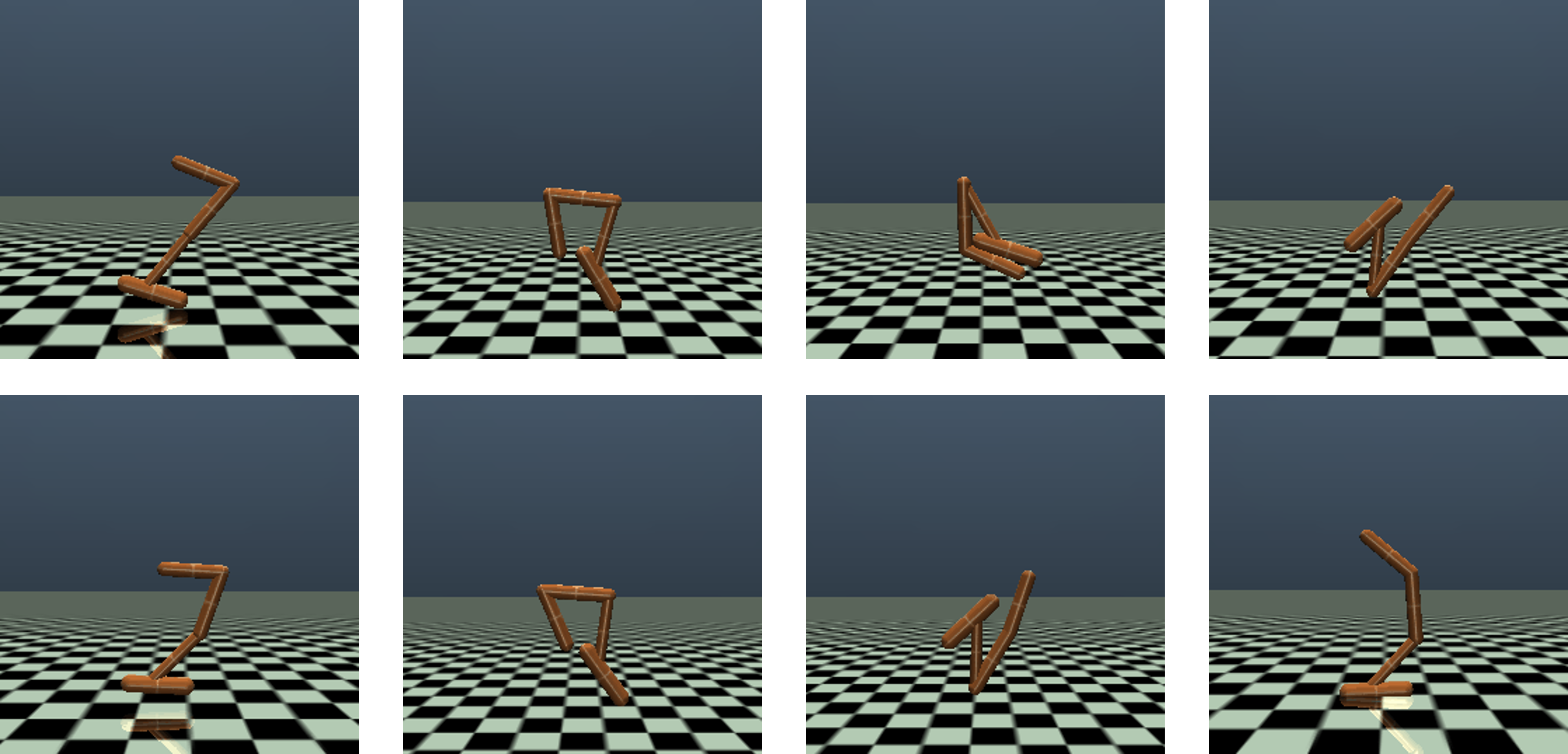
We employ a hand-crafted reward function designed by experts (Christiano et al., 2017) as the ground-truth scripted teacher. We find that compared to ground-truth preferences, the error rate of our non-expert annotations reached nearly 40%. The learning curves are shown in Fig. 5a. We find that RIME significantly outperforms PEBBLE when learning from actual non-expert human teachers and successfully performs consecutive backflips using 100 non-expert feedback, as shown in Figure 5b.

(a) Learning curves of RIME and PEBBLE on Hopper

(b) Frames of consecutive backflips from agents trained by RIME.

Figure 5: Ablation study on real non-expert human teachers

Component analysis. We perform ablation study to individually evaluate each technique in RIME: warm start (WS), lower bound $\tau_{\text{lower}}$, and upper bound $\tau_{\text{upper}}$ of KL divergence. We present results in Table 5 in which we compare the performance of removing each component from RIME. We observe that warm start is crucial for robustness when the number of feedback is quite limited (i.e.on Walker-walk). This is because the limited samples restrict the capability of the reward model, leading to more rounds of queries to cross the transition gap. Moreover, it might be hard to distinguish for discriminator at initial with limited samples, which urges for good initialized reward models.

The lower bound $\tau_{\text{lower}}$ for filtering trustworthy samples is important in high error rate ($\epsilon=0.3$ on Walker-walk and Button-press) and adequate feedback (on Button-press) situations. The upper bound $\tau_{\text{upper}}$ for flipping labels always brings some improvements in our ablation experiments. The full algorithm outperforms every other combination in most tasks. Additionally, the results show that although the contribution of warm start and denoising discriminator vary in different environments with low-level noise, they are both effective and their combination proves essential for the overall success of our method in environments with high-level noise.

Table 5: Ablation study of components in RIME on Walker and Button-press with different error rates, across 5 runs.

Component			Walker		Button Press
WS	$\tau_{\text{lower}}$	$\tau_{\text{upper}}$	$\epsilon=0.1$	$\epsilon=0.3$	$\epsilon=0.1$	$\epsilon=0.3$
✗	✗	✗	749 $\pm$ 123	431 $\pm$ 157	93.1 $\pm$ 10.6	22.0 $\pm$ 13.8
✗	✓	✓	688 $\pm$ 148	457 $\pm$ 190	97.2 $\pm$ 04.6	64.7 $\pm$ 26.5
✓	✗	✓	886 $\pm$ 070	492 $\pm$ 188	89.8 $\pm$ 11.5	35.1 $\pm$ 24.1
✓	✓	✗	842 $\pm$ 107	693 $\pm$ 167	96.9 $\pm$ 04.0	51.4 $\pm$ 30.0
✓	✓	✓	909 $\pm$ 132	741 $\pm$ 139	99.9 $\pm$ 00.3	80.0 $\pm$ 27.7

6 Conclusion

In this paper, we present RIME, a robust algorithm for preference-based reinforcement learning (PbRL) designed for effective reward learning from noisy preferences. Unlike previous research which primarily aims to enhance feedback efficiency, RIME focuses on improving robustness by employing a sample selection-based discriminator to dynamically denoise preferences. To reduce accumulated error due to incorrect selection, we utilize a warm-start method for the reward model, enhancing the initial capability of the denoising discriminator. The warm-start approach also serves to bridge the performance gap during transition, facilitating a seamless transition from pre-training to online training. Our experiments show that RIME substantially boosts the robustness of the state-of-the-art PbRL method across a range of complex robotic manipulation and locomotion tasks. Ablation studies further demonstrate that the warm-start approach is crucial for both robustness and feedback efficiency. We believe that RIME has the potential to broaden the applicability of PbRL by leveraging preferences from non-expert users or crowd-sourcing platforms.

Appendix A RIME Algorithm Details

In this section, we provide the full procedure for RIME based on the backbone PbRL algorithm, PEBBLE (Lee et al., 2021b), in Algorithm 1.

Algorithm 1 RIME

1:Initialize policy $\pi_{\phi}$, Q-network $Q_{\theta}$ and reward model $\hat{r}_{\psi}$

2:Initialize replay buffer $\mathcal{B}\leftarrow\emptyset$

3:// Unsupervised Pre-training

4:for each pre-training step $t$ do

5:     Collect $\mathbf{s}_{t+1}$ by taking $\mathbf{a}_{t}\sim\pi_{\phi}(\mathbf{a}_{t}|\mathbf{s}_{t})$

6:     Compute normalized intrinsic reward $r^{\text{int}}_{\text{norm},t}\leftarrow r^{\text{int}}_{\text{norm}}(\mathbf{s}_{t})$ as in Equation (9)

7:     Store transitions $\mathcal{B}\leftarrow\mathcal{B}\cup\left\{(\mathbf{s}_{t},\mathbf{a}_{t},\mathbf{s}_{t+1},r^{\text{int}}_{\text{norm},t})\right\}$

8:     for each gradient step do

9:         Sample minibatch $\left\{(\mathbf{s}_{j},\mathbf{a}_{j},\mathbf{s}_{j+1},r^{\text{int}}_{\text{norm},j})\right\}^{B}_{j=1}\sim\mathcal{B}$

10:         Optimize policy and Q-network with respect to $\phi$ and $\theta$ using SAC

11:         // Warm start

12:         Update reward model $\hat{r}_{\psi}$ according to Equation (10)

13:     end for

14:end for

15:// Online training

16:Initialize the maximum KL divergence value $\rho=\infty$

17:Initialize a dataset of noisy preferences $\mathcal{D}_{\text{noisy}}\leftarrow\emptyset$

18:for each training step $t$ do

19:     // Robust reward learning

20:     if $t\%K==0$ then

21:         Generate queries from replay buffer $\{(\sigma^{0}_{i},\sigma^{1}_{i})\}_{i=1}^{N_{\text{query}}}\sim\mathcal{B}$ and corresponding human feedback $\{\tilde{y}_{i}\}_{i=1}^{N_{\text{query}}}$

22:         Store preferences $\mathcal{D}_{\text{noisy}}\leftarrow\mathcal{D}_{\text{noisy}}\cup\{(\sigma^{0}_{i},\sigma^{1}_{i},\tilde{y}_{i})\}_{i=1}^{N_{\text{query}}}$

23:         Compute lower bound $\tau_{\text{lower}}$ according to Equation (5)

24:         Filter trustworthy samples $\mathcal{D}_{t}$ using lower bound $\tau_{\text{lower}}$ as in Equation (6)

25:         Flip labels using upper bound $\tau_{\text{upper}}$ to obtain dataset $\mathcal{D}_{f}$ as in Equation (7)

26:         Update reward model $\hat{r}_{\psi}$ with samples from $\mathcal{D}_{t}\cup\mathcal{D}_{f}$ according to Equation (8)

27:         Relabel entire replay buffer $\mathcal{B}$ using $\hat{r}_{\psi}$

28:         Update parameter $\rho$ with the maximum KL divergence between predicted and annotated labels in dataset $\mathcal{D}_{t}\cup\mathcal{D}_{f}$

29:     end if

30:     for each timestep $t$ do

31:         Collect $\mathbf{s}_{t+1}$ by taking $\mathbf{a}_{t}\sim\pi_{\phi}(\mathbf{a}_{t}|\mathbf{s}_{t})$

32:         Store transitions $\mathcal{B}\leftarrow\mathcal{B}\cup\{(\mathbf{s}_{t},\mathbf{a}_{t},\mathbf{s}_{t+1},\widehat{r}_{\psi}(\mathbf{s}_{t},\mathbf{a}_{t}))\}$

33:     end for

34:     for each gradient step do

35:         Sample minibatch from replay buffer $\{(\mathbf{s}_{j},\mathbf{a}_{j},\mathbf{s}_{j+1},\hat{r}_{\psi}(\mathbf{s}_{j},\mathbf{a}_{j})\}_{j=1}^{B}\sim\mathcal{B}$

36:         Optimize policy and Q-network with respect to $\phi$ and $\theta$ using SAC

37:     end for

38:end for

Appendix B Effects of biased reward model

Previous work empirically showed the detrimental impact of noisy preference on the reward model (Lee et al., 2021a). To further demonstrated the effects of a biased reward model, we introduce the following theorem and give the proof as follows.

Assumption B.1 (Fitting error of reward model).

Post the phase of reward learning, the fitting error between the learned reward model $\hat{r}_{\psi}$ and the ground-truth reward function $r^{*}$ within the state-action distribution encountered by policy $\pi$ is upper-bounded by a value $\delta$:

$$\operatorname*{\mathbb{E}}_{(\mathbf{s},\mathbf{a})\sim\rho^{\pi}}\left|\hat{r}_{\psi}(\mathbf{s},\mathbf{a})-r^{*}(\mathbf{s},\mathbf{a})\right|\leq\delta$$ (11)

Theorem B.2 (Upper bound of Q-function error).

Consider a Markov Decision Process characterized by the state transition function $P$, ground-truth reward function $r^{*}$, and discount factor $\gamma$. Let $Q^{\pi}$ denote the Q-function for policy $\pi$ with respect to the learned reward model $\hat{r}_{\psi}$. Then the error between $Q^{\pi}$ and the optimal Q-function $Q^{*}$ is upper-bounded by the fitting error $\delta$ of the reward model:

$$\operatorname*{\mathbb{E}}_{(\mathbf{s},\mathbf{a})\sim\rho^{\pi}}\left|Q^{\pi}(\mathbf{s},\mathbf{a})-Q^{*}(\mathbf{s},\mathbf{a})\right|\leq\frac{\delta}{1-\gamma\delta}$$ (12)

Proof.

$$\operatorname*{\mathbb{E}}_{(\mathbf{s},\mathbf{a})\sim\rho^{\pi}}\left|Q^{\pi}(\mathbf{s},\mathbf{a})-Q^{*}(\mathbf{s},\mathbf{a})\right|$$ (13)

$$= \operatorname*{\mathbb{E}}_{(\mathbf{s},\mathbf{a})\sim\rho^{\pi}}\left|\hat{r}_{\psi}(\mathbf{s},\mathbf{a})+\gamma\sum_{\mathbf{s}^{\prime}}P(\mathbf{s}^{\prime}|\mathbf{s},\mathbf{a})\sum_{\mathbf{a}^{\prime}}\pi(\mathbf{a}^{\prime}|\mathbf{s}^{\prime})Q^{\pi}(\mathbf{s}^{\prime},\mathbf{a}^{\prime})-r^{*}(\mathbf{s},\mathbf{a})-\gamma\sum_{\mathbf{s}^{\prime}}P(\mathbf{s}^{\prime}|\mathbf{s},\mathbf{a})\max_{\mathbf{a}^{\prime}}Q^{*}(\mathbf{s}^{\prime},\mathbf{a}^{\prime})\right|$$ (14)

$$\leq \operatorname*{\mathbb{E}}_{(\mathbf{s},\mathbf{a})\sim\rho^{\pi}}\left|\hat{r}_{\psi}(\mathbf{s},\mathbf{a})-r^{*}(\mathbf{s},\mathbf{a})\right|+\gamma\operatorname*{\mathbb{E}}_{(\mathbf{s},\mathbf{a})\sim\rho^{\pi}}\sum_{\mathbf{s}^{\prime}}P(\mathbf{s}^{\prime}|\mathbf{s},\mathbf{a})\left|\sum_{\mathbf{a}^{\prime}}\pi(\mathbf{a}^{\prime}|\mathbf{s}^{\prime})Q^{\pi}(\mathbf{s}^{\prime},\mathbf{a}^{\prime})-\max_{\mathbf{a}^{\prime}}Q^{*}(\mathbf{s}^{\prime},\mathbf{a}^{\prime})\right|$$ (15)

$$= \delta+\gamma\operatorname*{\mathbb{E}}_{(\mathbf{s},\mathbf{a})\sim\rho^{\pi}}\sum_{\mathbf{s}^{\prime}}P(\mathbf{s}^{\prime}|\mathbf{s},\mathbf{a})\left|\sum_{\mathbf{a}^{\prime}}\pi(\mathbf{a}^{\prime}|\mathbf{s}^{\prime})(Q^{\pi}(\mathbf{s}^{\prime},\mathbf{a}^{\prime})-\max_{\mathbf{a}^{\prime\prime}}Q^{*}(\mathbf{s}^{\prime},\mathbf{a}^{\prime\prime}))\right|$$ (16)

$$\leq \delta+\gamma\operatorname*{\mathbb{E}}_{(\mathbf{s},\mathbf{a})\sim\rho^{\pi}}\sum_{\mathbf{s}^{\prime}}P(\mathbf{s}^{\prime}|\mathbf{s},\mathbf{a})\sum_{\mathbf{a}^{\prime}}\pi(\mathbf{a}^{\prime}|\mathbf{s}^{\prime})(\max_{\mathbf{a}^{\prime\prime}}Q^{*}(\mathbf{s}^{\prime},\mathbf{a}^{\prime\prime})-Q^{\pi}(\mathbf{s}^{\prime},\mathbf{a}^{\prime}))$$ (17)

$$\leq \delta+\gamma\operatorname*{\mathbb{E}}_{(\mathbf{s},\mathbf{a})\sim\rho^{\pi}}\sum_{\mathbf{s}^{\prime}}P(\mathbf{s}^{\prime}|\mathbf{s},\mathbf{a})\sum_{\mathbf{a}^{\prime}}\pi(\mathbf{a}^{\prime}|\mathbf{s}^{\prime})(Q^{*}(\mathbf{s}^{\prime},\mathbf{a}^{\prime})-Q^{\pi}(\mathbf{s}^{\prime},\mathbf{a}^{\prime}))$$ (18)

$$= \delta+\gamma\operatorname*{\mathbb{E}}_{(\mathbf{s}^{\prime},\mathbf{a}^{\prime})\sim\rho^{\pi}}\left|Q^{\pi}(\mathbf{s}^{\prime},\mathbf{a}^{\prime})-Q^{*}(\mathbf{s}^{\prime},\mathbf{a}^{\prime})\right|$$ (19)

$$\leq \delta+\gamma\delta^{2}+\gamma^{2}\delta^{3}+\dots$$ (20)

$$\leq \frac{\delta}{1-\gamma\delta}$$ (21)

∎

Appendix C Proofs for Theorem 4

Theorem C.1.

Consider a preference dataset $\{(\sigma^{0}_{i},\sigma^{1}_{i},\tilde{y}_{i})\}_{i=1}^{n}$, where $\tilde{y}_{i}$ is the annotated label for the segment pair $(\sigma^{0}_{i},\sigma^{1}_{i})$ with the ground truth label $y_{i}$. Let $x_{i}$ denote the tuple $(\sigma^{0}_{i},\sigma^{1}_{i})$. Assume the cross-entropy loss $\mathcal{L}^{\mathtt{CE}}$ for clean data (whose $\tilde{y}_{i}=y_{i}$) within this distribution is bounded by $\rho$. Then, the KL divergence between the predicted preference $P_{\psi}(x)$ and the annotated label $\tilde{y}(x)$ for a corrupted sample $x$ is lower-bounded as follows:

$$D_{\mathrm{KL}}\left(P_{\psi}(x)\|\tilde{y}(x)\right)\geq-\ln\rho+\frac{\rho}{2}+\mathcal{O}(\rho^{2})$$ (22)

Proof.

For a clean sample $(\sigma^{0},\sigma^{1})$ with annotated label $\tilde{y}$ and ground-truth label $y$, we have $\tilde{y}=y$. Denote the predicted label as $P_{\psi}$. In PbRL, the value of $y(0)$ can take one of three forms: $y(0)\in\{0,0.5,1\}$. We categorize and discuss these situations as follows:

1. For $y(0)=0$:

   Because the cross-entropy loss $\mathcal{L}^{\mathtt{CE}}$ for clean data is bounded by $\rho$, we can express:

   $$\mathcal{L}^{\mathtt{CE}}(P_{\psi},\tilde{y})=-\ln(1-P_{\psi}(0))\leq\rho$$ (23)

   From the above, we have:

   $$P_{\psi}(0)\leq 1-\exp{(-\rho)}$$ (24)

   Then if the label is corrupted, denoted by $\tilde{y}_{c}$ (i.e.$\tilde{y}_{c}=(1,0)$ in this case), the KL divergence between predicted label and corrupted label is formulated as follows:

   $$D_{\mathrm{KL}}(P_{\psi}\|\tilde{y}_{c})=-\ln P_{\psi}(0)\geq-\ln(1-\exp(-\rho))$$ (25)

2. For $y(0)=1$:

   The discussion parallels the $y(0)=0$ case. Hence, the KL divergence between the predicted label and the corrupted label also maintains a lower bound:

   $$D_{\mathrm{KL}}(P_{\psi}\|\tilde{y}_{c})\geq-\ln(1-\exp(-\rho))$$ (26)

3. For $y(0)=0.5$:

   Although this case is not under the mistake model settings (Lee et al., 2021a), the lower bound still holds in this case. Due to the bounded cross-entropy loss $\mathcal{L}^{\mathtt{CE}}$ for clean data, we have:

   $$\mathcal{L}^{\mathtt{CE}}(P_{\psi},\tilde{y})=-\frac{1}{2}\ln P_{\psi}(0)-\frac{1}{2}\ln(1-P_{\psi}(0))\leq\rho$$ (27)

   Solving the inequality (27), we can get:

   $$P_{\psi}(0)^{2}-P_{\psi}(0)+\exp(-2\rho)\leq 0$$ (28)

   When $\rho\geq\ln 2$, the inequality (28) has a solution:

   $$1-p\leq P_{\psi}(0)\leq p$$ (29)

   where $p=\frac{1+\sqrt{1-4\exp(-2\rho)}}{2}$.

   Then if the label is corrupted, i.e.$\tilde{y}_{c}\in\{(0,1),(1,0)\}$, the KL divergence between predicted label and corrupted label is formulated as follows:

   $$D_{\mathrm{KL}}(P_{\psi}\|\tilde{y}_{c})\geq \min(-\ln P_{\psi}(0),-\ln(1-P_{\psi}(0)))=-\ln p$$ (30)

   Construct an equation about $\rho$:

   $$f(\rho)=p-1+\exp(-\rho)=\frac{1+\sqrt{1-4\exp(-2\rho)}}{2}-1+\exp(-\rho)$$ (31)

   where $\rho\geq\ln 2$.

   Denote $z=\exp(-\rho)$, Equation (31) can be simplified as follows:

   $$f(z)=z+\frac{\sqrt{1-4z^{2}}}{2}-\frac{1}{2}$$ (32)

   where $0<z\leq\frac{1}{2}$.

   Derivative of function $f$ with respect to $z$, we have:

   $$f^{{}^{\prime}}(z)=1-2\sqrt{\frac{1}{\frac{1}{z^{2}}-4}}$$ (33)

   Function $f^{{}^{\prime}}(z)$ decreases monotonically when $z\in(0,0.5]$, is greater than 0 on the interval $(0,\frac{\sqrt{2}}{4})$, and is less than 0 on the interval $(\frac{\sqrt{2}}{4},0.5]$. Therefore, we have:

   $$f(z)\leq\max(f(0),f(\frac{1}{2}))=0$$ (34)

   Thus, $p\leq 1-\exp(-\rho)$ when $\rho\geq\ln 2$. In turn, we have:

   $$D_{\mathrm{KL}}(P_{\psi}\|\tilde{y}_{c})=-\ln p\geq-\ln(1-\exp(-\rho))$$ (35)

To sum up, inequality (36) holds for the corrupted samples:

$$D_{\mathrm{KL}}(P_{\psi}\|\tilde{y}_{c})\geq-\ln(1-\exp(-\rho))$$ (36)

Perform Taylor expansion of the lower bound at $\rho=0$, we can get:

$$D_{\mathrm{KL}}(P_{\psi}\|\tilde{y}_{c})\geq-\ln(1-\exp(-\rho))=-\ln\rho+\frac{\rho}{2}+\mathcal{O}(\rho^{2})$$ (37)

∎

Appendix D Experimental Details

D.1 Tasks

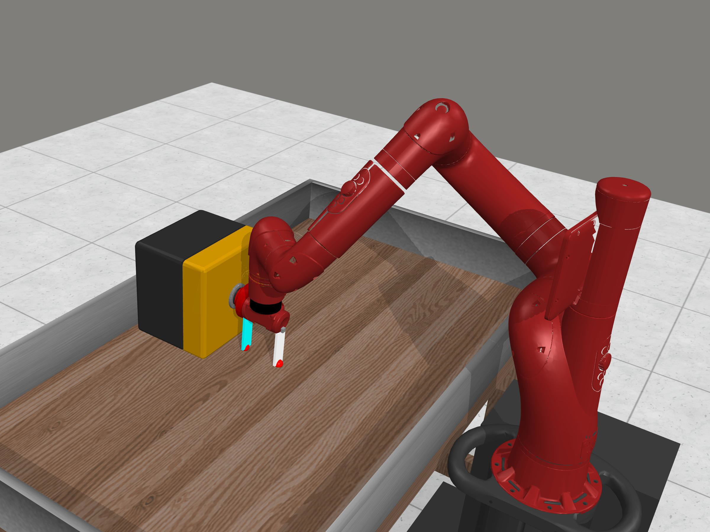
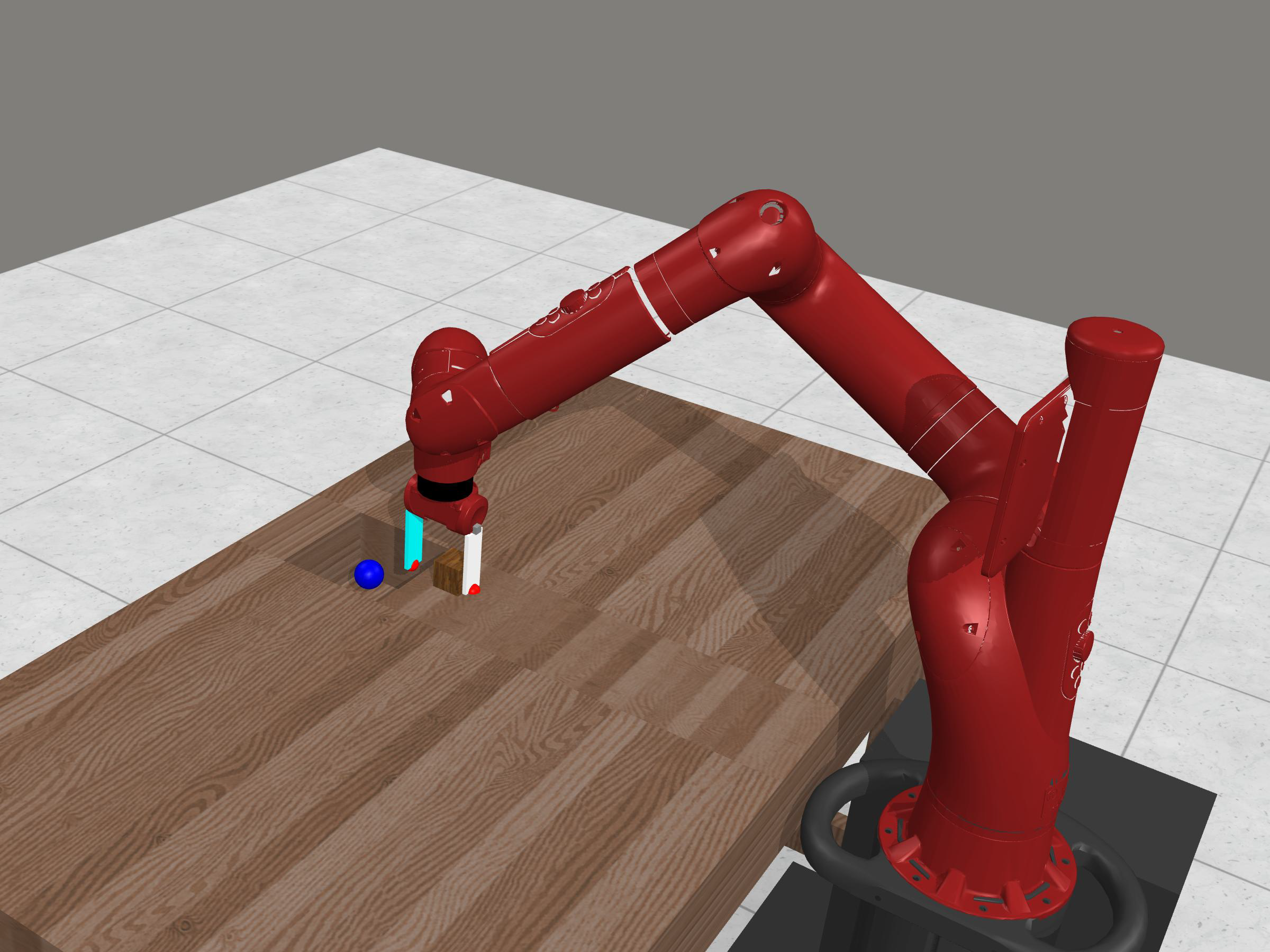
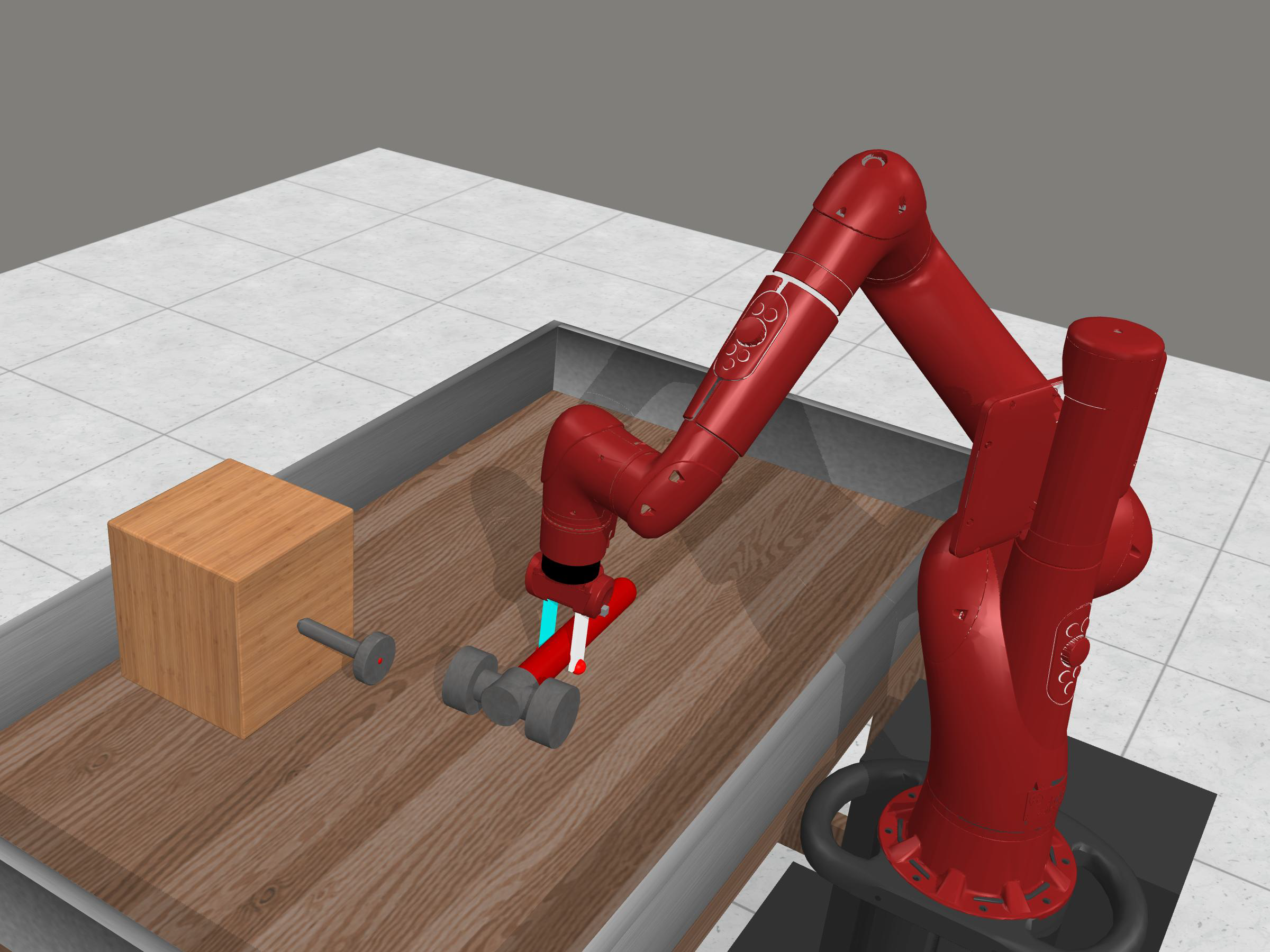
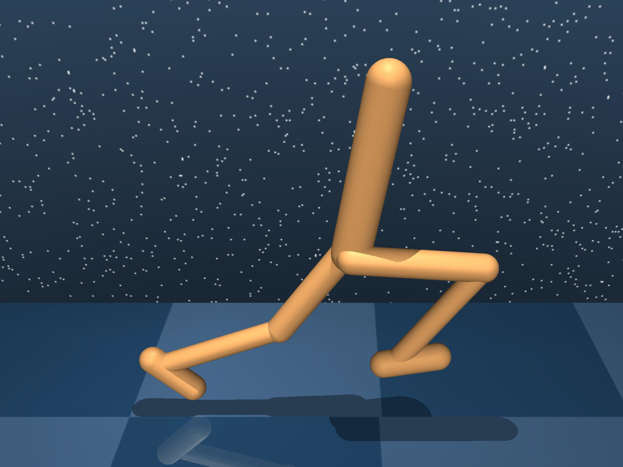
The robotic manipulation tasks from Meta-world (Yu et al., 2020) and locomotion tasks from DMControl (Tassa et al., 2018, 2020) used in our experiments are shown in Figure 6.

(a) Button Press

(b) Sweep Into

(c) Hammer

(d) Walker

(e) Cheetah

(f) Quadruped

Figure 6: Six tasks from Meta-world (a-c) and DMControl (d-f).

Meta-world Tasks:

1. Button Press: An agent controls a robotic arm to press a button. The button’s initial position is randomized.

2. Sweep Into: An agent controls a robotic arm to sweep a ball into a hole. The ball’s starting position is randomized.

3. Hammer: An agent controls a robotic arm to hammer a screw into a wall. The initial positions of both the hammer and the screw are randomized.

DMControl Tasks:

1. Walker: A planar walker is trained to control its body and walk on the ground.

2. Cheetah: A planar biped is trained to control its body and run on the ground.

3. Quadruped: A four-legged ant is trained to control its body and limbs, enabling it to crawl on the ground.

D.2 Implementation Details

For the implementation of baselines, we use their corresponding publicly released repositories that are shown in Table 6. SAC serves as a performance upper bound, because it uses a ground-truth reward function which is unavailable in PbRL settings for training. The detailed hyperparameters of SAC are shown in Table 7. PEBBLE’s settings remain consistent with its original implementation, and the specifics are detailed in Table 8. For SURF, RUNE, MRN, and RIME, most hyperparameters are the same as those of PEBBLE and other hyperparameters are detailed in Table 9, 10, 11, and 12, respectively. The total amount of feedback and feedback amount per session in each experimental condition are detailed in Table 1. The reward model comprises an ensemble of three MLPs. Each MLP consists of three layers with 256 hidden units, and the output of the reward model is constrained using the tanh activation function.

Table 6: Source codes of baselines.

Algorithm	Url
SAC, PEBBLE	https://github.com/rll-research/BPref
SURF	https://github.com/alinlab/SURF
RUNE	https://github.com/rll-research/rune
MRN	https://github.com/RyanLiu112/MRN

Table 7: Hyperparameters of SAC.

Hyperparameter	Value	Hyperparameter	Value
Number of layers	$2$ (DMControl), $3$ (Meta-world)	Initial temperature	$0.1$
Hidden units per each layer	$1024$ (DMControl), $256$ (Meta-world)	Optimizer	Adam
Learning rate	$0.0005$ (Walker), $0.001$ (Cheetah)	Critic target update freq	$2$
	$0.0001$ (Quadruped), $0.0003$ (Meta-world)	Critic EMA $\tau$	$0.005$
Batch Size	$1024$ (DMControl), $512$ (Meta-world)	$(\beta_{1},\beta_{2})$	$(0.9,0.999)$
Steps of unsupervised pre-training	$9000$	Discount $\gamma$	$0.99$

Table 8: Hyperparameters of PEBBLE.

Hyperparameter	Value
Segment Length	$50$
Learning rate	$0.0005$ (Walker, Cheetah), $0.0001$ (Quadruped), $0.0003$ (Meta-world)
Frequency of feedback	$20000$ (Walker, Cheetah), $30000$ (Quadruped), $5000$ (Meta-world)
Number of reward functions	$3$

Table 9: Hyperparameters of SURF.

Hyperparameter	Value
Unlabeled batch ratio $\mu$	$4$
Threshold $\tau$	$0.999$ (Cheetah, Sweep Into), $0.99$ (others)
Loss weight $\lambda$	1
Min/Max length of cropped segment	$45/55$
Segment length before cropping	$60$

Table 10: Hyperparameters of RUNE.

Hyperparameter	Value
Initial weight of intrinsic reward $\beta_{0}$	$0.05$
Decay rate $\rho$*	$0.001$ (Walker), $0.0001$ (Cheetah, Quadruped, Button Press)
	$0.00001$ (Sweep Into, Hammer)

*: Following the instruction of Liang et al. (2021), we carefully tune the hyperparameter $\rho$ in a range of $\rho\in\{0.001,0.0001,0.00001\}$ and report the best value for each environment.

Table 11: Hyperparameters of MRN.

Hyperparameter	Value
Bi-level updating frequency $N$	$5000$ (Cheetah, Hammer, Button Press), $1000$ (Walker)
	$3000$ (Quadruped), $10000$ (Sweep Into)

Table 12: Hyperparameters of RIME.

Hyperparameter	Value
Coefficient $\alpha$ in the lower bound $\tau_{\text{lower}}$	$0.5$
Minimum weight $\beta_{\min}$	1
Maximum weight $\beta_{\max}$	3
Decay rate $k$	1/30 (DMControl), 1/300 (Meta-world)
Upper bound $\tau_{\text{upper}}$	$3\ln(10)$
$\delta$ in Equation (9)	$1\times 10^{-8}$
Steps of unsupervised pre-training	$2000$ (Cheetah), $9000$ (others)

D.3 Details of scripted teachers

For a pair of trajectory segments $(\sigma^{0},\sigma^{1})$ with length $H$, where $\sigma^{i}=\{(\mathbf{s}_{1}^{i},\mathbf{a}^{i}_{1}),\dots,(\mathbf{s}_{H}^{i},\mathbf{a}_{H}^{i})\},(i=0,1)$. The ground-truth reward function from environment is $r(\mathbf{s},\mathbf{a})$. Then scripted teachers are defined as follows (Lee et al., 2021a):

Oracle: Oracle teacher provides ground-truth preferences. It prefers the segment with larger cumulative ground-truth rewards. For example, if $\sum_{i=1}^{H}r(\mathbf{s}^{0}_{i},\mathbf{a}^{0}_{i})>\sum_{i=1}^{H}r(\mathbf{s}^{1}_{i},\mathbf{a}^{1}_{i})$, then it returns the label as $(1,0)$.

Equal: Equal teacher gives equal preference $(0.5,0.5)$ if the difference between the cumulative rewards of two segments are small. In particular, if $|\sum_{t=1}^{H}r(\mathbf{s}_{t}^{1},\mathbf{a}_{t}^{1})-\sum_{t=1}^{H}r(\mathbf{s}_{t}^{0},\mathbf{a}_{t}^{0})|<\delta$, then it return the label $(0.5,0.5)$. $\delta=\frac{H}{T}R_{\text{avg}}\epsilon_{\text{adapt}}$, where T is the episode length, $R_{\text{avg}}$ is the average returns of current policy, $\epsilon_{\text{adapt}}$ is a hyperparameters and is set to 0.1 in experiments, following the setting in Lee et al. (2021a).

Skip: Skip teacher skips the query if the cumulative rewards of segments are small. In particular, if $\max_{i\in\{0,1\}}\sum_{t=1}^{H}r(\mathbf{s}_{t}^{i},\mathbf{a}_{t}^{i})<\delta$, then it will skip this query.

Myopic: Myopic teacher focuses more on the behavior at the end of segments. It prefers the segment with larger discounted cumulative ground-truth rewards. For example, if $\sum_{i=1}^{H}\gamma^{H-t}r(\mathbf{s}^{0}_{i},\mathbf{a}^{0}_{i})>\sum_{i=1}^{H}\gamma^{H-t}r(\mathbf{s}^{1}_{i},\mathbf{a}^{1}_{i})$, then it returns the label $(1,0)$.

Mistake: Mistake teacher flips the ground-truth preference labels with a probability of $\epsilon$.

D.4 Details of experiments with human teachers

Human experiments adopt an online paradigm consistent with PEBBLE’s pipeline, where agent training alternates with reward model training. When it is the timestep to collect preferences (post-agent training and pre-reward training), the training program generates segment pairs , saving each segment in GIF format. The program then pauses, awaiting the input of human preferences. At this juncture, human labelers engage, reading the paired segments in GIF format and labelling their preferences. Subsequently, this annotated data is fed into the training program for reward model training.

To ensure a fair comparison between RIME and PEBBLE, for one human labeler, we start the training programs for RIME and for PEBBLE simultaneously. When both training programs are waiting for inputting preferences, we collate all GIF pairs from both RIME and PEBBLE and shuffle the order. Then the human labeler starts working. Therefore, from the labeler’s perspective, he/she does not know which algorithm the currently labeled segment pair comes from and just focuses on labelling according to his/her preference. The labeled data is then automatically directed to the respective training programs. We conduct this experiment parallelly on each of the five labelers, thus preferences from different users do not get mixed.

In the Hopper task, the labeling process itself requires approximately 5 minutes, not accounting for waiting time. However, due to the online annotation, labelers experience downtime while waiting for agent training and GIF pair generation. Consequently, considering all factors, the total time commitment for labeling amounts to about 20 minutes per annotator.

Appendix E Additional Experiment Results

Effects of hyperparameters of RIME. We investigate how the hyperparameters of RIME affect the performance under noisy feedback settings. In Figure 7 we plot the learning curves of RIME with different set of hyperparameters: (a) coefficient $\alpha$ in the lower bound $\tau_{\text{lower}}$: $\alpha\in\{0.3,0.4,0.5,0.6\}$, (b) maximum value of $\beta_{t}$: $\beta_{\max}\in\{1,3,5,10\}$, (c) decay rate $k\in\{0.01,1/30,0.06,0.1\}$, and (d) upper bound of KL divergence $\tau_{\text{upper}}\in\{2\ln(10),3\ln(10),4\ln(10)\}$.

For the coefficient $\alpha$ in the lower bound $\tau_{\text{lower}}$, we find the theoretical value $\alpha=0.5$ performs the best. The maximum weight $\beta_{\max}$ and decay rate $k$ control the weight of uncertainty term in the lower bound $\tau_{\text{lower}}$: $\beta_{t}=\max(\beta_{\min},\beta_{\max}-kt)$. The combination of $\beta_{\max}=3$ and $k=1/30$ also performs optimally. Due to the quite limited feedback amount (1000 feedback) and training epochs for the reward model (around $150\sim 200$ epochs on Walker-walk), RIME is sensitive to the weight of uncertainty term. If ones try to increase $\beta_{\max}$ to add more tolerance for trustworthy samples in early-stage, we recommend to increase the decay rate $k$ simultaneously so that the value of $\beta_{t}$ decays to its minimum within about $1/3$ to $1/2$ of the total epochs. For the upper bound $\tau_{\text{upper}}$, although we use $3\ln(10)$ for balanced performance on DMControl tasks, individually fine-tuning $\tau_{\text{upper}}$ can further improve the performance of RIME on the corresponding task, such as using $\tau_{\text{upper}}=4\ln(10)$ for Walker-walk.

(a) Coefficient $\alpha$

(b) Maximum weight $\beta_{\max}$

(c) Decay rate $k$

(d) Upper bound $\tau_{\text{upper}}$

Figure 7: Hyperparameter analysis on Walker-walk using 1000 feedback with $\epsilon=0.3$. The results show the mean and standard deviation averaged over five runs.

Figure 8: Uncertainty term analysis on Walker-walk using 1000 feedback with $\epsilon=0.3$, across ten runs.

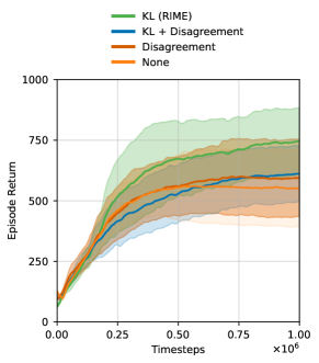
Effects of different uncertainty terms in the lower bound. In RIME, we use an auxiliary uncertainty term $\tau_{\text{unc}}$ in the lower bound $\tau_{\text{lower}}$ to accommodate tolerance during the early training stages and in cases of distribution shifts. The standard deviation of the KL divergence, denoted as the KL metric in this section, is employed to discern these cases. Here, we compare this with two other metrics: the disagreement metric and a combination of both, termed as KL + disagreement. The disagreement metric uses the standard deviation of $P_{\psi}[\sigma^{0}\succ\sigma^{1}]$ across the ensemble of reward models (denoted as $s_{P}$) to discern cases of distribution shifts: $\tau_{\text{unc}}=\gamma_{t}\cdot s_{P}$. Our intuition is that the predictions of the model for OOD data typically vary greatly. Notably, this metric induces sample-level, rather than buffer-level, thresholds, potentially offering more nuanced threshold control. The combined metric, KL + disagreement, integrates both as $\tau_{\text{unc}}=\beta_{t}\cdot s_{\text{KL}}+\gamma_{t}\cdot s_{P}$.

For reference, we also include a group devoid of any uncertainty term, termed the “None” group. As shown in Figure 8, the KL metric outperforms the other approaches on Walker-walk with an error rate of $\epsilon=0.3$. This might be because the disagreement metric fluctuates violently at every query times, often leading to excessive trust in new data, which hinders the stabilization of the lower bound.

References

- Agarwal et al. (2022) Agarwal, R., Schwarzer, M., Castro, P. S., Courville, A. C., and Bellemare, M. Reincarnating reinforcement learning: Reusing prior computation to accelerate progress. Advances in Neural Information Processing Systems, 35:28955–28971, 2022.
- Akrour et al. (2011) Akrour, R., Schoenauer, M., and Sebag, M. Preference-based policy learning. In Machine Learning and Knowledge Discovery in Databases: European Conference, ECML PKDD 2011, Athens, Greece, September 5-9, 2011. Proceedings, Part I 11, pp. 12–27. Springer, 2011.
- Bellemare et al. (2020) Bellemare, M. G., Candido, S., Castro, P. S., Gong, J., Machado, M. C., Moitra, S., Ponda, S. S., and Wang, Z. Autonomous navigation of stratospheric balloons using reinforcement learning. Nature, 588(7836):77–82, 2020.
- Bradley & Terry (1952) Bradley, R. A. and Terry, M. E. Rank analysis of incomplete block designs: I. the method of paired comparisons. Biometrika, 39(3/4):324–345, 1952.
- Chen et al. (2022) Chen, Y., Wu, T., Wang, S., Feng, X., Jiang, J., Lu, Z., McAleer, S., Dong, H., Zhu, S.-C., and Yang, Y. Towards human-level bimanual dexterous manipulation with reinforcement learning. Advances in Neural Information Processing Systems, 35:5150–5163, 2022.
- Cheng et al. (2020) Cheng, L., Zhou, X., Zhao, L., Li, D., Shang, H., Zheng, Y., Pan, P., and Xu, Y. Weakly supervised learning with side information for noisy labeled images. In European Conference on Computer Vision, pp. 306–321, 2020.
- Christiano et al. (2017) Christiano, P. F., Leike, J., Brown, T., Martic, M., Legg, S., and Amodei, D. Deep reinforcement learning from human preferences. Advances in Neural Information Processing Systems, 30, 2017.
- Feng et al. (2021) Feng, L., Shu, S., Lin, Z., Lv, F., Li, L., and An, B. Can cross entropy loss be robust to label noise? In Proceedings of the Twenty-Ninth International Conference on International Joint Conferences on Artificial Intelligence, pp. 2206–2212, 2021.
- Ghosh et al. (2017) Ghosh, A., Kumar, H., and Sastry, P. S. Robust loss functions under label noise for deep neural networks. In Proceedings of the AAAI conference on artificial intelligence, volume 31, 2017.
- Goldberger & Ben-Reuven (2016) Goldberger, J. and Ben-Reuven, E. Training deep neural-networks using a noise adaptation layer. In International Conference on Learning Representations, 2016.
- Grandvalet & Bengio (2004) Grandvalet, Y. and Bengio, Y. Semi-supervised learning by entropy minimization. Advances in Neural Information Processing Systems, 17, 2004.
- Hejna III & Sadigh (2023) Hejna III, D. J. and Sadigh, D. Few-shot preference learning for human-in-the-loop rl. In Conference on Robot Learning, pp. 2014–2025. PMLR, 2023.
- Ibarz et al. (2018) Ibarz, B., Leike, J., Pohlen, T., Irving, G., Legg, S., and Amodei, D. Reward learning from human preferences and demonstrations in atari. Advances in Neural Information Processing Systems, 31, 2018.
- Kaufmann et al. (2023) Kaufmann, E., Bauersfeld, L., Loquercio, A., Müller, M., Koltun, V., and Scaramuzza, D. Champion-level drone racing using deep reinforcement learning. Nature, 620(7976):982–987, 2023.
- Kim et al. (2022) Kim, C., Park, J., Shin, J., Lee, H., Abbeel, P., and Lee, K. Preference transformer: Modeling human preferences using transformers for rl. In International Conference on Learning Representations, 2022.
- Lee et al. (2021a) Lee, K., Smith, L., Dragan, A., and Abbeel, P. B-pref: Benchmarking preference-based reinforcement learning. In Thirty-fifth Conference on Neural Information Processing Systems Datasets and Benchmarks Track (Round 1), 2021a.
- Lee et al. (2021b) Lee, K., Smith, L. M., and Abbeel, P. Pebble: Feedback-efficient interactive reinforcement learning via relabeling experience and unsupervised pre-training. In International Conference on Machine Learning, pp. 6152–6163. PMLR, 2021b.
- Lee et al. (2023) Lee, K., Liu, H., Ryu, M., Watkins, O., Du, Y., Boutilier, C., Abbeel, P., Ghavamzadeh, M., and Gu, S. S. Aligning text-to-image models using human feedback. arXiv preprint arXiv:2302.12192, 2023.
- Li et al. (2020) Li, M., Soltanolkotabi, M., and Oymak, S. Gradient descent with early stopping is provably robust to label noise for overparameterized neural networks. In International Conference on Artificial Intelligence and Statistics, pp. 4313–4324. PMLR, 2020.
- Liang et al. (2021) Liang, X., Shu, K., Lee, K., and Abbeel, P. Reward uncertainty for exploration in preference-based reinforcement learning. In International Conference on Learning Representations, 2021.
- Liu & Abbeel (2021) Liu, H. and Abbeel, P. Behavior from the void: Unsupervised active pre-training. Advances in Neural Information Processing Systems, 34:18459–18473, 2021.
- Liu et al. (2022) Liu, R., Bai, F., Du, Y., and Yang, Y. Meta-reward-net: Implicitly differentiable reward learning for preference-based reinforcement learning. Advances in Neural Information Processing Systems, 35:22270–22284, 2022.
- Lukasik et al. (2020) Lukasik, M., Bhojanapalli, S., Menon, A., and Kumar, S. Does label smoothing mitigate label noise? In International Conference on Machine Learning, pp. 6448–6458. PMLR, 2020.
- Lyu & Tsang (2019) Lyu, Y. and Tsang, I. W. Curriculum loss: Robust learning and generalization against label corruption. In International Conference on Learning Representations, 2019.
- Ouyang et al. (2022) Ouyang, L., Wu, J., Jiang, X., Almeida, D., Wainwright, C., Mishkin, P., Zhang, C., Agarwal, S., Slama, K., Ray, A., et al. Training language models to follow instructions with human feedback. Advances in Neural Information Processing Systems, 35:27730–27744, 2022.
- Park et al. (2021) Park, J., Seo, Y., Shin, J., Lee, H., Abbeel, P., and Lee, K. Surf: Semi-supervised reward learning with data augmentation for feedback-efficient preference-based reinforcement learning. In International Conference on Learning Representations, 2021.
- Perolat et al. (2022) Perolat, J., De Vylder, B., Hennes, D., Tarassov, E., Strub, F., de Boer, V., Muller, P., Connor, J. T., Burch, N., Anthony, T., et al. Mastering the game of stratego with model-free multiagent reinforcement learning. Science, 378(6623):990–996, 2022.
- Singh et al. (2003) Singh, H., Misra, N., Hnizdo, V., Fedorowicz, A., and Demchuk, E. Nearest neighbor estimates of entropy. American journal of mathematical and management sciences, 23(3-4):301–321, 2003.
- Song et al. (2021) Song, H., Kim, M., Park, D., Shin, Y., and Lee, J.-G. Robust learning by self-transition for handling noisy labels. In Proceedings of the 27th ACM SIGKDD Conference on Knowledge Discovery & Data Mining, pp. 1490–1500, 2021.
- Song et al. (2022) Song, H., Kim, M., Park, D., Shin, Y., and Lee, J.-G. Learning from noisy labels with deep neural networks: A survey. IEEE Transactions on Neural Networks and Learning Systems, 2022.
- Sutton & Barto (2018) Sutton, R. S. and Barto, A. G. Reinforcement learning: An introduction. MIT press, 2018.
- Tassa et al. (2018) Tassa, Y., Doron, Y., Muldal, A., Erez, T., Li, Y., Casas, D. d. L., Budden, D., Abdolmaleki, A., Merel, J., Lefrancq, A., et al. Deepmind control suite. arXiv preprint arXiv:1801.00690, 2018.
- Tassa et al. (2020) Tassa, Y., Tunyasuvunakool, S., Muldal, A., Doron, Y., Trochim, P., Liu, S., Bohez, S., Merel, J., Erez, T., Lillicrap, T., et al. dm_control: Software and tasks for continuous control. arXiv preprint arXiv:2006.12983, 2020.
- Uchendu et al. (2023) Uchendu, I., Xiao, T., Lu, Y., Zhu, B., Yan, M., Simon, J., Bennice, M., Fu, C., Ma, C., Jiao, J., et al. Jump-start reinforcement learning. In International Conference on Machine Learning, pp. 34556–34583. PMLR, 2023.
- Vinyals et al. (2019) Vinyals, O., Babuschkin, I., Czarnecki, W. M., Mathieu, M., Dudzik, A., Chung, J., Choi, D. H., Powell, R., Ewalds, T., Georgiev, P., et al. Grandmaster level in starcraft ii using multi-agent reinforcement learning. Nature, 575(7782):350–354, 2019.
- Wang et al. (2021) Wang, W., Feng, F., He, X., Nie, L., and Chua, T.-S. Denoising implicit feedback for recommendation. In Proceedings of the 14th ACM international conference on web search and data mining, pp. 373–381, 2021.
- Wei et al. (2021) Wei, J., Liu, H., Liu, T., Niu, G., Sugiyama, M., and Liu, Y. To smooth or not? when label smoothing meets noisy labels. arXiv preprint arXiv:2106.04149, 2021.
- Xia et al. (2020) Xia, X., Liu, T., Han, B., Gong, C., Wang, N., Ge, Z., and Chang, Y. Robust early-learning: Hindering the memorization of noisy labels. In International Conference on Learning Representations, 2020.
- Xue et al. (2023) Xue, W., An, B., Yan, S., and Xu, Z. Reinforcement learning from diverse human preferences. arXiv preprint arXiv:2301.11774, 2023.
- Yu et al. (2020) Yu, T., Quillen, D., He, Z., Julian, R., Hausman, K., Finn, C., and Levine, S. Meta-world: A benchmark and evaluation for multi-task and meta reinforcement learning. In Conference on Robot Learning, pp. 1094–1100. PMLR, 2020.
- Zhang & Sabuncu (2018) Zhang, Z. and Sabuncu, M. Generalized cross entropy loss for training deep neural networks with noisy labels. Advances in Neural Information Processing Systems, 31, 2018.
- Zhou et al. (2020) Zhou, M., Luo, J., Villella, J., Yang, Y., Rusu, D., Miao, J., Zhang, W., Alban, M., Fadakar, I., Chen, Z., et al. Smarts: Scalable multi-agent reinforcement learning training school for autonomous driving. arXiv preprint arXiv:2010.09776, 2020.