Inverse Optimal Control for Linear Quadratic Tracking with Unknown Target States

Abstract

This paper addresses the inverse optimal control for the linear quadratic tracking problem with a fixed but unknown target state, which aims to estimate the possible triplets comprising the target state, the state weight matrix, and the input weight matrix from observed optimal control input and the corresponding state trajectories. Sufficient conditions have been provided for the unique determination of both the linear quadratic cost function as well as the target state. A computationally efficient and numerically reliable parameter identification algorithm is proposed by equating optimal control strategies with a system of linear equations, and the associated relative error upper bound is derived in terms of data volume and signal-to-noise ratio. Moreover, the proposed inverse optimal control algorithm is applied for the joint cluster coordination and intent identification of a multi-agent system. By incorporating the structural constraint of the Laplace matrix, the relative error upper bound can be reduced accordingly. Finally, the algorithm’s efficiency and accuracy are validated by a vehicle-on-a-lever example and a multi-agent formation control example.

I Introduction

Inverse Optimal Control (IOC), pioneered by [10], aims to identify the underlying reward or penalty mechanism implicit in a policy by observing optimal control trajectories. It bears similarity to inverse reinforcement learning, where a structural parametrization is assumed for the performance index function and the parameters are then identified based on optimal input and state trajectories. Thus, the IOC problem can be regarded as the gray-box identification problem, facilitating the transfer of empirical knowledge to analogous scenarios with practical value of new dynamics. Its applications can be found in robotics [24, 6, 38, 26, 20] and beyond [40, 25, 12].

Based on different performance index functions, optimal control and the corresponding IOC problems can be classified into finite-horizon and infinite-horizon scenarios, where the former often yield time-variant strategies, while the latter exhibit the opposite. Various effective methods have been proposed for infinite-horizon IOC problems, as observed in [5, 13, 14, 15]. In [37], IOC for averaged cost per stage linear quadratic regulators is explored, considering both process and observation noises. For finite-horizon IOC problems, a few approaches based on open-loop information structures, such as Pontryagin’s maximum principle, have been proposed in [2, 3, 4]. The IOC problems for nonlinear systems have been investigated in [21, 22, 23, 39], while studies on IOC problems related to partial state observations can be found in [6, 7, 8, 9, 33, 34]. Despite the advancements, many existing identification methods are developed without considering the process and observation noises. In the presence of only observation noise, the identification method [38] demonstrates that consistent results can be obtained when the number of trajectories tend to infinity. However, when both process noise and observation noise are present, finite-horizon IOC methods utilizing open-loop information structures may encounter challenges [36].

The simplicity and broad applicability of linear quadratic optimal control have resulted in a multitude of related IOC applications [28, 29, 27, 16]. In recent years, IOC methods have been developed for linear quadratic tracking (LQT) optimal control, with research on IOC for LQT in continuous-time infinite-horizon scenarios conducted in [17, 30]. Additionally, [31] presents a data-driven IOC method for LQT in discrete-time infinite-horizon settings, which does not require system dynamics information. Finite-horizon LQT-IOC problems for state feedback control and output feedback control are explored in [38] and [11], respectively. Challenges arise when the target state is unknown, given the coupling between the target state and the state weight matrix in the LQT performance index function.

This paper focuses on solving the IOC for LQT within the discrete-time finite-horizon scenario, aiming to jointly determine the state weight matrix, the input weight matrix, and the target state. The concerned IOC problem is tackled by equivalently transforming the optimal control policy into linear equations. Addressing the coupling term in the LQT performance index function involves initially determining the state weight matrix and input weight matrix, followed by estimating the target state from a specific solution space. When parameters have structural prior information, reducing error can be achieved through projection techniques. For the optimal formation control problem, the Laplacian matrix generates state weight matrices with duplicate and zero elements, which can be projected through (half-)vectorization operations, to maintain linearity in solving the IOC problem.

The contributions of this paper are summarized as follows:

(i) Sufficient identifiability conditions and a linear estimation algorithm are provided for joint identification of the target state, state weight matrix, and input weight matrix in the presence of process noise. In addition, theoretical guarantees regarding the relative error upper bound are derived in terms of data volume and signal-to-noise ratio.

(ii) The specialization of the proposed method is demonstrated in the IOC of the multi-agent formation control with unknown fixed interconnection topology. It is theoretically shown that integrating structural prior knowledge can reduce algorithmic errors, illustrating the extensibility of the proposed method in high-dimensional systems with certain structural information.

The remainder of the paper unfolds as follows. Section II outlines the problem. The identifiability is analyzed in Section III. Section IV presents the algorithm and its theoretical guarantees. Section V applies the method to topology identification. The simulation is provided in Section VI and Section VII concludes the paper.

Notations: $I_{n}$ denotes an $n\times n$ identity matrix and $0_{n\times p}$ denotes the zero matrix; their subscripts are omitted when confusion is not caused. $\mathbf{1}_{N}$ denotes an $N$-dimensional vector with all elements being $1$. $\mathbb{R}^{n}$ denotes the $n$-dimensional linear space defined over the real numbers. $\mathbb{S}^{n}$, $\mathbb{S}_{+}^{n}$, and $\mathbb{S}_{++}^{n}$ denote the sets of symmetric matrices, positive semi-definite symmetric matrices, and positive definite symmetric matrices of dimension $n$, respectively. $\otimes$ denotes the Kronecker product. If $A\in\mathbb{R}^{n\times n}$, then $vec(A)$ and $vech(A)$ is the $n^{2}$-by-$1$ and $n(n+1)/2$-by-$1$ vectors obtained by stacking the columns of $A$ and the lower triangular part of $A$, respectively. For any matrix $A\in\mathbb{S}^{n}$, the duplication matrix $\mathcal{D}_{n}$ is used to transform half-vectorization into vectorization, i.e., $\mathcal{D}_{n}vech(A)=vec(A)$. Use $A^{\dagger}$ and $\mathcal{P}^{\text{ker}(A)}=I-A^{\dagger}A$ to denote the pseudoinverse matrix and the projection operator onto the kernel space of matrix $A$, respectively. $A^{-1}$ denotes the inverse matrix of invertible matrix $A$. $A^{\top}$ denotes the transpose of $A$ and $\|\cdot\|$ denotes the $L_{2}$ norm. The condition number of the matrix $A$ with full column rank is denoted as $\text{cond}(A)$, which is defined with respect to the $L_{2}$ norm and equals the ratio of its largest and smallest singular values. $\mathbb{E}$ denotes the expectation. $\text{diag}({\phi})$ denotes the diagonal matrix with vector $\phi$ as its diagonal.

II Problem Formulation

In this paper, the optimal control for the discrete-time finite-horizon linear quadratic tracking problem with process noise is considered:

$$\min_{\begin{subarray}{c}u_{k}\end{subarray}}\qquad {\mathbb{E}}\left\{\sum_{k={0}}^{{K}}e_{k+1}^{\top}Qe_{k+1}+u_{k}^{\top}Ru_{k}\right\}$$ (1a)

$$s.t.\qquad x_{k+1}=Ax_{k}+Bu_{k}+w_{k}$$ (1b)

$$e_{k+1}=x_{k+1}-d,\quad k=0,1,\cdots,K$$ (1c)

where $x_{k}\in\mathbb{R}^{n}$ and $u_{k}\in\mathbb{R}^{p}$ represent the system’s state and control input, respectively. $e_{k}$ denotes the residual between the state $x_{k}$ and the target state $d$. The process noise $w_{k}$ is a zero-mean random vector with finite second moment. The system matrix $A$, input matrix $B$, state weight matrix $Q$, and input weight matrix $R$ are conformable matrices, and $K$ denotes the control horizon, a finite value. For the above optimal control problem, assuming the initial state $x_{0}$ is known, the following assumption is made and a lemma will be provided to show the optimal control policy.

Assumption 1

The weight matrix $Q$ is positive semidefinite symmetric and $R$ is positive definite symmetric, i.e. $Q\in\mathbb{S}_{+}^{n},R\in\mathbb{S}_{++}^{p}$.

Lemma 1

Consider the optimal control problem (1). Under Assumption 1, given $x_{0},A,B,Q,R,d$, if $w_{k}$ is uncorrelated with $x_{k},u_{k}$, then the optimal control input $u_{k}$ is given by

$$u_{k}=\pi_{k}(Q,R,d,x_{k})$$ (2)

where

$$\pi_{k}(Q,R,d,x_{k}) =\begin{bmatrix}\Psi_{k}(Q,R)&\psi_{k}(Q,R,d)\end{bmatrix}\begin{bmatrix}x_{k}\\ 1\end{bmatrix}$$ (3a)

$$\Psi_{k}(Q,R) =-(R+B^{\top}P_{k+1}B)^{-1}B^{\top}P_{k+1}A$$ (3b)

$$\psi_{k}(Q,R,d) =-(R+B^{\top}P_{k+1}B)^{-1}B^{\top}\eta_{k+1}$$ (3c)

and $P_{k}$, $\eta_{k}$ are determined by the following Riccati equations

$$\eta_{k} =q+A^{\top}(P_{k+1}B\psi_{k}+\eta_{k+1})$$ (4a)

$$P_{k} =Q+A^{\top}(P_{k+1}B\Psi_{k}+P_{k+1}A)$$ (4b)

with $q=-Qd$ and the terminal conditions $\eta_{K+1}=q,P_{K+1}=Q$.

The proof of Lemma 1 can be found in Appendix A.

Remark 1

Although the state transition equation in (1b) contains the process noise, it does not appear in the optimal control policy; therefore, it does not need to be specially dealt with. Moreover, although the target state $d$ and the state weight matrix $Q$ are coupled together in (1a), they are individually separated in the optimal control policy, thus facilitating the inverse identification problem.

Before the addressed IOC problem is formally described, the following assumptions are introduced.

Assumption 2

The matrix pair $(A,B)$ is controllable. Moreover, $A$ is invertible and $B$ has full column rank.

Assumption 3

The control horizon satisfies $K\geq 2n$.

The reasonableness of the above assumptions is supported by [7], [33], [36]. Identifying the reward or cost associated with the mentioned optimal control requires multiple trajectories of data. This paper addresses the following problem:

Problem 1

Given $T$ sets of optimal input and state trajectories of length $K$, denoted as $\{x_{t,k},u_{t,k}\}_{k=0,t=1}^{K,T}$, the concerned IOC problem aims to find the possible triplets $(Q,R,d)$ satisfying $u_{t,k}=\pi_{k}(Q,R,d,x_{t,k})$ under Assumptions 1-3. Furthermore, let $\theta=\begin{bmatrix}(vech(R))^{\top}&(vech(Q))^{\top}&q^{\top}\end{bmatrix}^{\top}$. If prior knowledge $C\theta=c$ is given, where $c\neq 0$, it aims to find a particular solution for the constrained IOC problem.

Throughout the rest of this paper, for brevity, the subscript $t$ will be omitted when unnecessary.

In the subsequent sections, the well-posedness of Problem 1 is firstly discussed, and identifiability conditions for parameters are laid out. Then, leveraging the established conditions, an efficient and numerically reliable identification algorithm is proposed. Additionally, theoretical guarantees on the IOC results will be elucidated when the number of trajectories tends to infinity.

III Identifiability analysis

For given $x_{k}$ and any $\alpha>0,\lambda\in\mathbb{R}^{n}$, the triplet $(Q,R,d)$ generates the same $u_{k}$ as $(\alpha Q,\alpha R,d+\mathcal{P}^{\text{ker}(Q)}\lambda)$ does, due to the form of cost (1a), where $\mathcal{P}^{\text{ker}(Q)}=I-Q^{\dagger}Q$. In other words, parameters of this form constitute solutions to the concerned IOC problems.

The following theorem provides sufficient identifiability conditions for the concerned IOC problem.

Theorem 1

Given data $\{x_{t,k},u_{t,k}\}_{k=0,t=1}^{K,T}$ strictly adhering to (2) with unknown $(Q,R,d)$, the following conditions hold:

(i) Assumptions 1-3 are satisfied;

(ii) $\mathcal{Q}=BR^{-1}B^{\top}+Q\in\mathbb{S}_{++}^{n}$ and $\mathcal{Q}A\neq A\mathcal{Q}$;

(iii) For any $k=0,1,\cdots,{K}$, the matrix $X_{k}$ has full row rank, where

$$X_{k}=\begin{bmatrix}x_{1,k}&x_{2,k}&\cdots&x_{T,k}\\ 1&1&\cdots&1\end{bmatrix}$$

Then, the solution $(\hat{Q},\hat{R},\hat{d},\hat{P}_{k},\hat{\eta}_{k})$ to

$$(\hat{R}+B^{\top}\hat{P}_{k+1}B)u_{k}+B^{\top}\hat{P}_{k+1}Ax_{k}+B^{\top}\hat{\eta}_{k+1}=0$$ (5a)

$$A^{\top}\hat{P}_{k+1}Bu_{k}+(\hat{Q}+A^{\top}\hat{P}_{k+1}A-\hat{P}_{k})x_{k}$$

$$\qquad+\hat{q}+A^{\top}\hat{\eta}_{k+1}-\hat{\eta}_{k}=0$$ (5b)

$$\hat{P}_{K+1}=\hat{Q}$$ (5c)

$$\hat{\eta}_{K+1}=\hat{q}=-\hat{Q}\hat{d}$$ (5d)

satisfies $\hat{Q}=\alpha Q,\hat{R}=\alpha R,\alpha\neq 0$. Furthermore, if $Q$ and $d$ comply with $\mathcal{P}^{ker(Q)}d=0$, then $\hat{d}=d$.

Proof:

Through straightforward algebraic manipulation, it is evident that equation (5) and equation (2) are equivalent and share the same solutions. As a consequence, the solution to (2) will be investigated in order to derive the sufficient conditions.

Given $\{u_{k},x_{k}\}$ satisfying (2), every $u_{k}$ is a linear combination of $\begin{bmatrix}(x_{k})^{\top}&1\end{bmatrix}^{\top}$, i.e., there exist matrices $G_{k}$ and vectors $g_{k}$ such that

$$u_{k}=\begin{bmatrix}G_{k}&g_{k}\end{bmatrix}\begin{bmatrix}x_{k}\\ 1\end{bmatrix}$$ (6)

By substituting (6) into equations (5a) and (5b), the following equations are derived.

$$(\Gamma_{1,k}+\Gamma_{2,k})X_{k} =0,\quad k=0,1,\cdots,K$$ (7a)

$$(\Gamma_{3,k}+\Gamma_{4,k})X_{k} =0,\quad k=1,2,\cdots,K$$ (7b)

where

$$\Gamma_{1,k} =(R+B^{\top}P_{k+1}B)\begin{bmatrix}G_{k}&g_{k}\end{bmatrix}$$

$$\Gamma_{2,k} =\begin{bmatrix}B^{\top}P_{k+1}A&B^{\top}\eta_{k+1}\end{bmatrix}$$

$$\Gamma_{3,k} =A^{\top}P_{k+1}B\begin{bmatrix}G_{k}&g_{k}\end{bmatrix}$$

$$\Gamma_{4,k} =\begin{bmatrix}Q+A^{\top}P_{k+1}A-P_{k}&q+A^{\top}\eta_{k+1}-\eta_{k}\end{bmatrix}$$

Since every $X_{k}$ has full row rank, there holds that

$$\Gamma_{1,k}+\Gamma_{2,k} =0$$ (8a)

$$\Gamma_{3,k}+\Gamma_{4,k} =0$$ (8b)

With (8a) and $R+B^{\top}P_{k+1}B\in\mathbb{S}_{++}^{n}$, it is obviously that

$$G_{k} =-(R+B^{\top}P_{k+1}B)^{-1}B^{\top}P_{k+1}A$$ (9a)

$$g_{k} =-(R+B^{\top}P_{k+1}B)^{-1}B^{\top}\eta_{k+1}$$ (9b)

According to (8b), $P_{k}$ and $\eta_{k}$ satisfy

$$\eta_{k} =q+A^{\top}(P_{k+1}Bg_{k}+\eta_{k+1})$$ (10a)

$$P_{k} =Q+A^{\top}(P_{k+1}BG_{k}+P_{k+1}A)$$ (10b)

Suppose that there are two triplets $(Q,R,d)$ and $(\hat{Q},\hat{R},\hat{d})$ such that

$$u_{k}=\pi_{k}(Q,R,d,x_{k}) =\pi_{k}(\hat{Q},\hat{R},\hat{d},x_{k})$$ (11)

which means that the two triplets lead to the same $u_{k}$ for $x_{k}$. Considering all the given data, equations (11) and (3a) imply that

$$\begin{bmatrix}\Psi_{k}(Q,R)-\Psi_{k}(\hat{Q},\hat{R})&\psi_{k}(Q,R,d)-\psi_{k}(\hat{Q},\hat{R},\hat{d})\end{bmatrix}X_{k}=0$$ (12)

Given that for $k=0,1,\cdots,{K}$, each $X_{k}$ has a full row rank, it follows that

$$\Psi_{k}(Q,R) =\Psi_{k}(\hat{Q},\hat{R})$$ (13)

$$\psi_{k}(Q,R,d) =\psi_{k}(\hat{Q},\hat{R},\hat{d})$$ (14)

By left-multiplying both sides of (13) with $B$ and adding $A$, it can be obtained that

$$A+B\Psi_{k}(Q,R)=A+B\Psi_{k}(\hat{Q},\hat{R})$$ (15)

Applying the Woodbury matrix identity, it can be derived from (3b) and (15) that

$$(I+BR^{-1}B^{\top}P_{k+1})^{-1}A=(I+B\hat{R}^{-1}B^{\top}\hat{P}_{k+1})^{-1}A$$ (16)

Recall Assumption 2, which states that $A$ is invertible and $B$ has full column rank. It can be verified with (16) that

$$R^{-1}B^{\top}P_{k} =\hat{R}^{-1}B^{\top}\hat{P}_{k}$$ (17)

Further, based on Theorem 1 in [33], there exists a non-zero scalar $\alpha$ such that

$$\alpha Q =\hat{Q}$$ (18)

$$\alpha R =\hat{R}$$ (19)

The equations (17) and (19) lead to

$$\alpha B^{\top}P_{k+1} =B^{\top}\hat{P}_{k+1}$$ (20)

$$\alpha P_{k+1}B =\hat{P}_{k+1}B$$ (21)

Then, equations (19) and (20) establish the following relationship:

$$\alpha(\hat{R}+B^{\top}\hat{P}_{k+1}B)^{-1} =(R+B^{\top}P_{k+1}B)^{-1}$$ (22)

Define $\Delta\eta_{k+1}=\alpha\eta_{k+1}-\hat{\eta}_{k+1}$ and $\Delta q=\Delta\eta_{K+1}=\alpha q-\hat{q}$. Substituting the equations (3c) and (22) into (14) yields that

$$B^{\top}\Delta\eta_{k+1} =0$$ (23)

Moreover, with equations (4a), (14) and (21), it has that

$$\Delta\eta_{k} =\Delta q+A^{\top}\Delta\eta_{k+1}$$ (24)

According to (23) and (24), the conclusion can be drawn that

$$\Delta q^{\top}\begin{bmatrix}B&AB&\cdots&A^{K}B\end{bmatrix}=0$$ (25)

Since the system is controllable and $K\geq 2n>n-p$, it can be concluded that $\Delta q=0$, i.e. $\alpha q=\hat{q}$. Based on (18) and $\hat{q}=-\hat{Q}\hat{d}$, if $\mathcal{P}^{ker(\hat{Q})}\hat{d}=(I-\hat{Q}^{\dagger}\hat{Q})\hat{d}=0$, then $d=\hat{Q}^{\dagger}\hat{Q}\hat{d}=\hat{d}$. This completes the proof. ∎

Remark 2

Except for $q=-Qd$, equation (5) consists of a group of linear equations with respect to $Q,R,q,P_{k},\eta_{k}$. As a result, the matrices $Q$ and $R$ can be determined up to a scalar ambiguity. However, when the target state $d$ is in the range of $Q$, it can be uniquely determined. The outcomes derived from Theorem 1 signify that solving the IOC problem entails solving a semidefinite programming task with linear equality constraints. Practical implementations can be facilitated through software toolkits such as Yalmip or CVX.

The condition (iii) in Theorem 1 is a persistently exciting condition, which can be guaranteed as shown in the following lemma.

Lemma 2

Under Assumptions 1-3, if the process noise terms $w_{k}$ are uncorrelated with states and inputs, and $x_{0}$ is an independent identically distributed (i.i.d.) random vector following the distribution $x_{0}\sim\mathcal{N}(0,\Sigma_{0})$, then for any $k=0,\cdots,K$, $X_{k}$ almost surely has full row rank.

Proof:

According to equations (1b), (2) and (3a), it can be derived that

$$X_{k+1}=\begin{bmatrix}A+B\Psi_{k}(Q,R)&B\psi_{k}(Q,R,d)\\ 0&1\end{bmatrix}X_{k}+\begin{bmatrix}w_{k}\\ 0\end{bmatrix}$$ (26)

In the proof of Theorem 1, when deriving (16) from (15), the invertibility of $A+B\Psi_{k}(Q,R)$ has been verified, following the Woodbury matrix identity, for the matrix $R+B^{\top}P_{k+1}B$ is invertible. Besides, in line with the Schur complement condition, it can be established that

$$\begin{bmatrix}A+B\Psi_{k}(Q,R)&B\psi_{k}(Q,R,d)\\ 0&1\end{bmatrix}$$

is invertible. As a result, it has been shown that when $X_{k}$ has full row rank, $X_{k+1}$ is almost surely full row rank due to the related assumptions on $w_{k}$. In addition, as the initial state $x_{0}$ is a random vector following the distribution $x_{0}\sim\mathcal{N}(0,\Sigma_{0})$, the matrix $X_{0}$ has full row rank almost surely. Therefore, the proposition is proved by induction. ∎

IV Identification algorithm

In practice, the optimal input and state trajectories are observed with noise perturbation; as a result, the corresponding input and state data do not strictly satisfy (5). This section presents an estimation algorithm to obtain reliable numerical solutions.

IV-A Reformulation of linear equations

An analytical solution to equations in (5) will be provided through a linearization approach.

For simplicity, the term $Ax_{k}+Bu_{k}$ in equation (1b) will be denoted as $y_{k}$. Rewriting (5a) and (5b) with respect to unknown matrices and vectors yields that

$$Ru_{k}+B^{\top}P_{k+1}y_{k}+B^{\top}\eta_{k+1}=0$$ (27a)

$$Qx_{k}+q+A^{\top}P_{k+1}y_{k}+A^{\top}\eta_{k+1}-P_{k}x_{k}-\eta_{k}=0$$ (27b)

The above equation can be linearized as:

$$(u_{k}\otimes I)^{\top}vec(R)+B^{\top}(y_{k}\otimes I)^{\top}vec(P_{k+1})+B^{\top}\eta_{k+1}=0$$ (28a)

$$(x_{k}\otimes I)^{\top}vec(Q)+q+A^{\top}(y_{k}\otimes I)^{\top}vec(P_{k+1})+A^{\top}\eta_{k+1}$$

$$\qquad-(x_{k}\otimes I)^{\top}vec(P_{k})-\eta_{k}=0$$ (28b)

Since that $Q,R,P_{k}\in\mathbb{S}^{n}$, with half-vectorization, the equations above can be simplified as

$$(u_{k}\otimes I)^{\top}\mathcal{D}_{p}vech(R)+B^{\top}(y_{k}\otimes I)^{\top}\mathcal{D}_{n}vech(P_{k+1})$$

$$+B^{\top}\eta_{k+1}=0$$ (29a)

$$(x_{k}\otimes I)^{\top}\mathcal{D}_{n}vech(Q)+q+A^{\top}(y_{k}\otimes I)^{\top}\mathcal{D}_{n}vech(P_{k+1})$$

$$+A^{\top}\eta_{k+1}-(x_{k}\otimes I)^{\top}\mathcal{D}_{n}vech(P_{k})-\eta_{k}=0$$ (29b)

where the duplication matrices $\mathcal{D}_{n},\mathcal{D}_{p}$ have full column rank. To obtain a triplet $(Q,R,q)$ satisfying (5), vectors

$$\theta=\begin{bmatrix}(vech(R))^{\top}&(vech(Q))^{\top}&q^{\top}\end{bmatrix}^{\top}$$

and

$$r_{k}=\begin{bmatrix}(vech(P_{k}))^{\top}&\eta_{k}^{\top}\end{bmatrix}^{\top}$$

are introduced. Consequently, the system of linear equations can be expressed in the following compact form:

$$\begin{bmatrix}\Phi_{u,k}&0\end{bmatrix} \theta+\Phi_{B,k}\Phi_{y,k}r_{k+1}=0,\ k=0,\cdots,K$$ (30a)

$$\begin{bmatrix}0&\Phi_{x,k}\end{bmatrix} \theta+\Phi_{A,k}\Phi_{y,k}r_{k+1}=\Phi_{x,k}r_{k},\ k=1,\cdots,K$$ (30b)

$$\begin{bmatrix}0&I\end{bmatrix} \theta=r_{K+1}$$ (30c)

where

$$\Phi_{B,k} =I_{T}\otimes B^{\top}$$ (31a)

$$\Phi_{A,k} =I_{T}\otimes A^{\top}$$ (31b)

$$\Phi_{u,k} =\left(\begin{bmatrix}u_{1,k}&u_{2,k}&\cdots&u_{T,k}\end{bmatrix}\otimes I\right)^{\top}\mathcal{D}_{p}$$ (31c)

$$\Phi_{y,k} =\left(\begin{bmatrix}y_{1,k}&y_{2,k}&\cdots&y_{T,k}\\ 1&1&\cdots&1\end{bmatrix}\otimes I\right)^{\top}\tilde{\mathcal{D}}_{n}$$ (31d)

$$\Phi_{x,k} =\left(X_{k}\otimes I\right)^{\top}\tilde{\mathcal{D}}_{n}$$ (31e)

$$\tilde{\mathcal{D}}_{n} =\begin{bmatrix}\mathcal{D}_{n}&\\ &I\end{bmatrix}$$ (31f)

In order to obtain an estimate of $\theta$, $r_{k}$ is to be eliminated from equation (30). By introducing

$$r=\begin{bmatrix}r_{1}^{\top}&r_{2}^{\top}&\cdots&r_{{K}}^{\top}\end{bmatrix}^{\top}$$ (32)

it can be derived from (30) that

$$\begin{bmatrix}\Phi_{U}&\Phi_{Y0}\\ 0&\Phi_{X}\end{bmatrix}\theta+\begin{bmatrix}\Phi_{Y1}\\ \Phi_{Y2}\end{bmatrix}r=0$$ (33)

where

$$\Phi_{U}=\begin{bmatrix}\Phi_{u,0}\\ \vdots\\ \Phi_{u,{K}}\end{bmatrix}$$ (34a)

$$\Phi_{Y0}=\begin{bmatrix}0\\ \vdots\\ 0\\ \Phi_{B,{K}}\Phi_{y,{K}}\end{bmatrix}$$ (34b)

$$\Phi_{X}=\begin{bmatrix}\Phi_{x,0}\\ \vdots\\ \Phi_{x,K-1}\\ \Phi_{x,{K}}+\Phi_{A,{K}}\Phi_{y,{K}}\end{bmatrix}$$ (34c)

$$\Phi_{Y1}=\begin{bmatrix}0&\Phi_{B,0}\Phi_{y,0}&&\\ \vdots&\ddots&\ddots&\\ &&0&\Phi_{B,{K}}\Phi_{y,K-1}\\ 0&\cdots&0&0\end{bmatrix}$$ (34d)

$$\Phi_{Y2}=\begin{bmatrix}-\Phi_{x,0}&\Phi_{A,0}\Phi_{y,0}&&&\\ &-\Phi_{x,1}&\ddots&\\ &&\ddots&\Phi_{A,K-1}\Phi_{y,K-1}\\ &&&-\Phi_{x,{K}}\end{bmatrix}$$ (34e)

Since the duplication matrix $\mathcal{D}_{n}$ has full column rank, $\tilde{\mathcal{D}}_{n}$ also has full column rank by (31f). Therefore, $\Phi_{x,k}$ has full column rank according to (31e). As implied by (34e), $\Phi_{Y2}$ has full column rank, and $r=-\Phi_{Y2}^{\dagger}\Phi_{X}r_{K+1}$ if and only if $\Phi_{X}r_{K+1}+\Phi_{Y2}r=0$. Substituting the expression of $r$ in terms of $\theta$, (33) can be rewritten as

$$Z\theta=0$$ (35a)

$$Z=\begin{bmatrix}\Phi_{U}&\Phi_{Y0}-\Phi_{Y1}\Phi_{Y2}^{\dagger}\Phi_{X}\\ 0&(I-\Phi_{Y2}\Phi_{Y2}^{\dagger})\Phi_{X}\end{bmatrix}$$ (35b)

The solution $\theta$ can be obtained from the linear equation (35a). Due to the homogeneity of the equation (35a), the solution set of $\theta$ can be determined by the kernel of $Z$.

Next, considering the constraint $C\theta=c$, the solutions to the IOC problem will be investigated.

By combining a nonhomogeneous linear constraint $C\tilde{\theta}=c$ with $Z\tilde{\theta}=0$, a nonhomogeneous linear system of equations with respect to $\tilde{\theta}$ is established as follows

$$\begin{bmatrix}C\\ H\end{bmatrix}\tilde{\theta}=\begin{bmatrix}c\\ 0\end{bmatrix}$$ (36)

where $H=Z^{\top}Z/T$. When the coefficient matrix of the above equation has full column rank, there exists a unique solution

$$\tilde{\theta}=\begin{bmatrix}C\\ H\end{bmatrix}^{\dagger}\begin{bmatrix}c\\ 0\end{bmatrix}$$ (37)

During the construction of $Z$, all the operations are sufficient and necessary under the conditions in Theorem 1, so $Z$ and $H=Z^{\top}Z/T$ is rank deficient by one, and $H\tilde{\theta}=0$ determines $\tilde{\theta}$ up to a scalar ambiguity. For $\theta=\alpha\tilde{\theta}$, $0\neq c=C\theta=C\alpha\tilde{\theta}$ holds if and only if $\alpha=1$, i.e. $\theta=\tilde{\theta}$. In other words, the coefficient matrix $\begin{bmatrix}C^{\top}&H\end{bmatrix}^{\top}$ has full column rank when $c\neq 0$.

Theorem 1 offers a theoretical guarantee, ensuring that $Z$ takes continuous values with respect to the trajectory sequence, thereby laying the foundation for error analysis. The The implementation process of the algorithm is summarized in Algorithm 1.

Algorithm 1 Inverse LQT with target state identified

Given $A,B,u_{k}$ and $x_{k}$.

 

Step 1: Linear equations construction

(1) Select $T$ pairs of the optimal control input and the corresponding state such that $X_{k}$ has full row rank for each time $k={0},1,\cdots,{K}$;

(2) Compute $y_{k}=Ax_{k}+Bu_{k}$ with selected data;

(3) Calculate the intermediate variables $\Phi_{u,k},\Phi_{x,k},\Phi_{y,k}$ according to equation (31);

(4) Construct the data matrices $\Phi_{U},\Phi_{X},\Phi_{Y0},\Phi_{Y1},\Phi_{Y2}$ according to equation (34);

(5) Obtain the coefficient matrix $Z$ according to (35b) and then $H=Z^{\top}Z/T$.

 

Step 2: Particular solution acquisition

(1) Figure out $\tilde{\theta}$ from (37);

(2) Restructure $(\tilde{Q},\tilde{R},\tilde{q})$ with $\tilde{\theta}$, and then $\tilde{d}=-\tilde{Q}^{\dagger}\tilde{q}$.

 

All the solutions are $(\alpha\tilde{Q},\alpha\tilde{R},\tilde{d}+\mathcal{P}^{\text{ker}\tilde{Q}}\lambda),\alpha>0,\lambda\in\mathbb{R}^{n}$.

IV-B Error analysis

This paper proposes a numerically reliable and computational efficient algorithm for which some interesting statistical properties will be analyzed.

Recall Problem 1 when $T\to\infty$ and observation noises exist, denote the observed state and input trajectories as

$$\{\tilde{x}_{t,k},\tilde{u}_{t,k}\}_{k=0,t=1}^{K,T}=\{x_{t,k}+\Delta x_{t,k},u_{t,k+}\Delta u_{t,k}\}_{k=0,t=1}^{K,T}$$

where $\Delta x_{t,k},\Delta u_{t,k}$ denote the observation noise terms.

To make more explicitly use of the assumption regarding observation noises, the following analysis is based on (33).

When the conditions of Theorem 1 are satisfied, the IOC problem can be addressed by solving the following equation

$$C\tilde{\theta}=c$$ (38a)

$$\frac{1}{T}\begin{bmatrix}\tilde{\Phi}_{U}&\tilde{\Phi}_{Y0}&\tilde{\Phi}_{Y1}\\ 0&\tilde{\Phi}_{X}&\tilde{\Phi}_{Y2}\end{bmatrix}^{\top}\begin{bmatrix}\tilde{\Phi}_{U}&\tilde{\Phi}_{Y0}&\tilde{\Phi}_{Y1}\\ 0&\tilde{\Phi}_{X}&\tilde{\Phi}_{Y2}\end{bmatrix}\begin{bmatrix}\tilde{\theta}\\ \tilde{r}\end{bmatrix}=0$$ (38b)

where the soution $\tilde{\theta}$ can be obtaned with Algorithm 1 equivalently. Let

$$\tilde{z}=\begin{bmatrix}\tilde{\theta}\\ \tilde{r}\end{bmatrix}$$ (39)

and (38) can be rewritten in the following compact form

$$\tilde{\Omega}\tilde{z}=\begin{bmatrix}c\\ 0\end{bmatrix}$$ (40)

In accordance with (31)-(34), there exist $\Omega$ and $\Delta{\Omega}$ such that

$$\tilde{\Omega} =\Omega+\frac{1}{T}\Delta{\Omega}$$ (41)

where the term $\Delta{\Omega}$ is attributed to observation noises. It is divided by $T$ because it represents the aggregate of the observation noise terms $\Delta x_{t,k},\Delta u_{t,k}$ acting in $\tilde{\Omega}$, and is scaled by the data volume $T$ during the construction of the coefficient matrix $\tilde{\Omega}$. In contrast, the term $\Omega$ represents the ultimately obtained effective signal data, as the defination below. Define the signal-to-noise ratio (SNR) as

$$\text{SNR}=10\text{log}\frac{\left\|\Omega\right\|}{\left\|\Delta{\Omega}\right\|}$$ (42)

and define the estimation errors of $\tilde{\theta}$ and $\tilde{z}$ as

$$\Delta{\theta} =\tilde{\theta}-{\theta}$$ (43a)

$$\Delta{z} =\tilde{z}-{z}$$ (43b)

where ${\theta}$ and $z$ are the true values.

The above definitions allows us to analyze the statistical properties of the solutions to the concerned IOC problem.

Theorem 2

Given $T$ sets of trajectories meeting the conditions in Theorem 1, if the observation noise has a mean of $0$ with finite second moment, then Algorithm 1 yields a consistent estimate $\tilde{\theta}$. Moreover, when $T\to\infty$ the relative error satisfies

$$\frac{\|\Delta{\theta}\|}{\|{\theta}\|}\leq\frac{\|z\|}{\|{\theta}\|}T^{-0.5}\text{cond}(\Omega)10^{-0.1\text{SNR}}$$ (44)

Proof:

According to (39) and (43), it is clear that

$$\frac{\|\Delta{\theta}\|}{\|{\theta}\|}=\frac{\|z\|}{\|{\theta}\|}\frac{\|\Delta{\theta}\|}{\|z\|}\leq\frac{\|z\|}{\|{\theta}\|}\frac{\|\Delta{z}\|}{\|z\|}$$ (45)

It then follows from (40), (41) and (43b) that

$$\tilde{\Omega}\tilde{z}=(\Omega+\frac{1}{T}\Delta{\Omega})(z+\Delta{z})=\Omega z$$ (46)

Note that the observation noise has a mean of $0$ with finite second moment, then

$$\lim_{T\to\infty}\frac{1}{T}\Delta{\Omega}=0, \lim_{T\to\infty}\Omega\tilde{z}=\lim_{T\to\infty}\Omega{z}$$ (47)

Since $\Omega$ has full column rank, there holds

$$\lim_{T\to\infty}\Delta{z}=0, \mathbb{E}\{\tilde{z}\}=z$$ (48)

which indicates that $\tilde{\theta}$ is indeed a consistent estimate.

Moreover, via trivial algebraic manipulations, equation (46) implies that

$$T\Delta z=-(\Omega+\frac{1}{T}\Delta{\Omega})^{\dagger}\Delta{\Omega}z$$ (49)

Taking the $L_{2}$ norm on both sides of (49), in line with the compatibility of the $L_{2}$ norm with the matrix $L_{2}$ norm, we can obtain that

$$\|T\Delta z\|\leq\left\|(\Omega+\frac{1}{T}\Delta{\Omega})^{\dagger}\right\|\|\Delta{\Omega}\|\|z\|$$ (50)

In the light of the monotonicity property of limits, it can be concluded that

$$\lim_{T\to\infty}\|T\Delta z\|\leq\lim_{T\to\infty}\left\|(\Omega+\frac{1}{T}\Delta{\Omega})^{\dagger}\right\|\|\Delta{\Omega}\|\|z\|$$ (51)

which yields

$$\frac{\|\Delta{z}\|}{\|z\|} \leq\left\|\frac{1}{T}\right\|\left\|\Omega^{\dagger}\right\|\left\|\Omega\right\|\frac{\left\|\Delta{\Omega}\right\|}{\left\|\Omega\right\|}$$ (52)

$$=T^{-0.5}\text{cond}(\Omega)10^{-0.1\text{SNR}}$$ (53)

as $T\to\infty$. This completes the proof of the theorem. ∎

Remark 3

The above theorem shows that, for a given SNR, the convergence rate is indeed $\mathcal{O}(T^{-0.5})$, as conjectured in [35]. Based on the equivalence between dynamic programming and Riccati equations, the proposed method in this paper does not necessitate knowledge of the statistical properties of observation noises, which are required as priori knowledge in the SDP method [35].

The multiplier $\text{cond}(\Omega)$ indicates that $n+1$ orthogonal $\begin{bmatrix}x_{k}^{\top}&1\end{bmatrix}^{\top}$ vectors help to ensure $\text{cond}(\Omega)=1$, and increasing $T$ contributes to making $\text{cond}(\Omega)$ closer to this lower bound.

V Multi-agent LQT formation under fixed but unknown topology

In this section, the framework proposed in this paper will demonstrate its specialization for multi-agent LQT under fixed but unknown topology, to explore the coordination pattern and intents of networked agents. For each intelligent agent $j$, its state $x_{k}^{j}\in\mathbb{R}^{n_{0}}$ constitutes a part of the cluster state $x_{k}$, where $j=1,2,\cdots,N$, and similarly the input $u_{k}^{j}\in\mathbb{R}^{p_{j}}$ constitutes a stacked vector $u_{k}$, namely

$$x_{k}=\begin{bmatrix}x_{k}^{1}\\ \vdots\\ x_{k}^{N}\end{bmatrix}\in\mathbb{R}^{n} u_{k}=\begin{bmatrix}u_{k}^{1}\\ \vdots\\ u_{k}^{N}\end{bmatrix}\in\mathbb{R}^{p}$$ (54)

where $n={Nn_{0}}$, $p={\sum_{j=1}^{N}{p_{j}}}$.

The dynamics of the entire cluster consists of the following dynamics of individual agents:

$$x_{k+1}^{j}=A_{j}x_{k}^{j}+B_{j}u_{k}^{j}+w_{k}^{j}$$

with their intent $d$ collectively described by the target states $d^{j}\in\mathbb{R}^{n_{0}}$ of each agent $j$. In this setting, the behavior and performance of multi-agents adhere to (1), where

$$A=\begin{bmatrix}A_{1}&&\\ &\ddots&\\ &&A_{N}\end{bmatrix} B=\begin{bmatrix}B_{1}&&\\ &\ddots&\\ &&B_{N}\end{bmatrix} \quad d=\begin{bmatrix}d^{1}\\ \vdots\\ d^{N}\end{bmatrix}$$ (55)

Likewise, the policy for multi-agent LQT formation under fixed but unknown topology can also be characterized according to (2) and obtained by minimizing the cost function (1a), and

$$Q ={(L+I)}\otimes I_{n_{0}}$$ (56a)

$$R =\text{diag}(\phi),\quad\phi\in\mathbb{R}^{p}$$ (56b)

where $L$ denotes the Laplacian matrix for multi-agent system, representing the network topology; the weight matrix R is a diagonal matrix, representing the input energy cost of individual agents. Following the setting in [32], where the topology of multi-agents forms a connected undirected graph, $L$ possesses the following properties.

(i) $L\in\mathbb{S}_{+}^{N}$;

(ii) $\mathbf{1}_{N}^{\top}L=0$.

Problem 2

Consider the multi-agent LQT formation policy $\pi_{k}$ in (2) under fixed but unknown topology, with $Q$ and $R$ being defined in (56). Given $T$ sets of optimal state and input trajectories with length $K$, i.e., $\{x_{t,k},u_{t,k}\}_{k=0,t=1}^{K,T}$, the concerned IOC problem aims to find $(L,\phi,d)$ satisfying $u_{k}=\pi_{k}\left({(L+I)}\otimes I,\text{diag}(\phi),d,x_{k}\right)$.

To further analyze the identifiability and errors of Problem 2, structural prior knowledge of $Q$ and $R$ will be adopted, ensuring a unique triplet $(Q,R,d)$ leads to the unique $(L,\phi,d)$ accordingly.

As discussed above regarding Theorem 1 and Algorithm 1, obtaining a unique pair $(Q,R)$ crucially relies on finding constraints $C\theta=c$, where $c\neq 0$. Furthermore, ensuring a unique $d$ requires $\mathcal{P}^{\text{ker}(Q)}d=0$. These conditions can be replaced by the properties of $L$.

Lemma 3

[19]. For $L+I$, there exist $\mathcal{F},\mathcal{H}$ such that

$$vec({(L+I)}\otimes I)=(I\otimes\mathcal{F})vec({(L+I)})$$ (57)

where

$$\mathcal{F} =(\mathcal{H}\otimes I)(I\otimes vec(I))$$ (58)

$\mathcal{H}$ is the commutation matrix that transforms the vectorized form of a matrix into the vectorized form of its transpose, and $I\otimes\mathcal{F}$ has full column rank.

Based on Theorem 1 and Lemma 3, the following corollary can be obtained.

Corollary 1

Consider the Problem 2 with $Q={(L+I)}\otimes I$ where $L\in\mathbb{S}_{+}^{n}$ and $\mathbf{1}_{N}^{\top}L=0$. Let

$$C=\begin{bmatrix}0_{N\times p(p+1)/2}&(I\otimes\mathbf{1}_{N}^{\top})(I\otimes\mathcal{F})^{\dagger}\mathcal{D}_{n}&0_{N\times n}\end{bmatrix}$$ (59)

with $c=\mathbf{1}_{N}$, where $\mathcal{F}$ is defined in (58). If the conditions of Theorem 1 hold, the solution $(\tilde{L},\tilde{\phi},\tilde{d})$ to (37) satisfies that $\tilde{L}=L,\tilde{\phi}=\phi$ and $\tilde{d}=d$, where $L,\phi,d$ are the true values.

Proof:

To prove $\tilde{L}=L$ and $\tilde{\phi}=\phi$, it suffices to demonstrate that $\tilde{Q}=Q$ and $\tilde{R}=R$.

Recall the previous discussion on (37), since $c=\mathbf{1}_{N}\neq 0$, it suffices to show that for the proposed $C$ and $c$, the $\theta$ obtained from $(Q,R,d)$ satisfies $C{\theta}=c$.

As per (56a), the linearization of $Q$ signifies that

$$vec(Q) =vec({(L+I)}\otimes I)$$ (60)

Substituting it into $C\theta$ yields that

$$C\theta=\begin{bmatrix}0_{N\times p(p+1)/2}&(I\otimes\mathbf{1}_{N}^{\top})(I\otimes\mathcal{F})^{\dagger}\mathcal{D}_{n}&0_{N\times n}\end{bmatrix}\theta$$

$$=\begin{bmatrix}0_{N\times p(p+1)/2}&(I\otimes\mathbf{1}_{N}^{\top})(I\otimes\mathcal{F})^{\dagger}\mathcal{D}_{n}&0_{N\times n}\end{bmatrix}\begin{bmatrix}vech(R)\\ vech(Q)\\ q\end{bmatrix}$$

$$=(I\otimes\mathbf{1}_{N}^{\top})(I\otimes\mathcal{F})^{\dagger}vec({(L+I)}\otimes I)$$

$$=(I\otimes\mathbf{1}_{N}^{\top})vec({L+I})$$

$$=vec(\mathbf{1}_{N}^{\top}(L+I))$$

$$=\mathbf{1}_{N}$$

$$=c$$

Hence, $\tilde{Q}=Q$ and $\tilde{R}=R$, then $\tilde{L}=L$ and $\tilde{\phi}=\phi$ hold true, as established by Theorem 1 and (56). Furthermore, since $L\in\mathbb{S}_{+}^{N}$, it implies that $Q={(L+I)}\otimes I\in\mathbb{S}_{++}^{n}$. Consequently, from $\mathcal{P}^{\text{ker}(Q)}d=0$, we conclude $\tilde{d}=d$ by Theorem 1. This completes the proof of the corollary. ∎

It is apparent that the well-posedness of Problem 2 is guaranteed by the distinctive structure of $Q=(L+I)\otimes I$. Subsequently, the particular configurations of $Q$ and $R$ will be concurrently exploited to develop a more efficient and accurate method addressing Problem 2.

Let

$$\bar{\theta}=\begin{bmatrix}\phi^{\top}&(vech(L+I))^{\top}&q\end{bmatrix}^{\top}$$

and according to (56) and (57), it can be obtained that

$$\theta=\begin{bmatrix}vech(\text{diag}(\phi))\\ D_{n}^{\dagger}(I\otimes\mathcal{F})\mathcal{D}_{N}vech(L+I)\\ q\end{bmatrix}$$ (61)

then $\theta$ can be reconstructed after the identification of $\bar{\theta}$.

Redefine

$$\Phi_{u,k} =\left(\begin{bmatrix}\text{diag}(u_{1,k})&\cdots&\text{diag}(u_{T,k})\end{bmatrix}\otimes I\right)^{\top}\mathcal{D}_{p}$$ (62a)

$$\tilde{D}_{n} =\begin{bmatrix}(I\otimes\mathcal{F})\mathcal{D}_{N}&\\ &I\end{bmatrix}$$ (62b)

$$C =\begin{bmatrix}0_{N\times p}&(I\otimes\mathbf{1}_{N}^{\top})\mathcal{D}_{N}&0_{N\times n}\end{bmatrix}$$ (62c)

with $c=\mathbf{1}_{N}$, then an estimate of $\bar{\theta}$ can be obtained according to Algorithm 1, from which a new estimate $\hat{\theta}$ can be reconstructed by (61).

The estimation process of $\hat{\theta}$ proves to be more efficient than that of acquiring $\tilde{\theta}$ as outlined in Corollary 1. This enhanced efficiency stems from a reduction in the dimensionality of the coefficient matrix in the linear equations. Furthermore, the approach ensures greater accuracy by precisely fulfilling the structural prior knowledge, under observation noises.

Proposition 1

Suppose that the observation noise is zero-mean with finite second moment. Let $\hat{\theta}$ denote the estimate by Algorithm 1 with (61)-(62), and $\tilde{\theta}$ be estimated from (31) and (59), then

$$\|\hat{\theta}-{\theta}\|^{2}=\|\tilde{\theta}-\theta\|^{2}-\|\tilde{\theta}-\hat{\theta}\|^{2}$$ (63)

where $\theta$ denotes the true value.

Proof:

Following (61)-(62), the procedure of obtaining $\hat{\theta}$ ensures that the duplicate and zero elements in $Q={(L+I)}\otimes I,R=\text{diag}(\phi)$ adhere to their structural characteristics, which can be expressed using the linear constraint $V\theta=v$. The resulting $\hat{\theta}$ strictly satisfies this linear equality constraint, i.e.

$$V\hat{\theta}=v$$ (64)

Denote $\Delta H$ as the noise term w.r.t $H$ defined in Algorithm 1 and (31), then $\hat{\theta}$ is the solution to the following optimization problem

$$\begin{split}\min_{\begin{subarray}{c}\hat{\theta}\end{subarray}}\quad\|S\hat{\theta}&-s\|^{2}\\ s.t.\ \quad V\hat{\theta}&=V\theta=v\\ S&=\begin{bmatrix}C^{\top}&{H}^{\top}+\Delta H^{\top}\end{bmatrix}^{\top}\\ s&=\begin{bmatrix}\mathbf{1}_{N}^{\top}&0\end{bmatrix}^{\top}\end{split}$$ (65)

with $C$ defined in (59). Since $S\tilde{\theta}=s$ and $S$ has full column rank, $\hat{\theta}$ is also the solution of the following optimization problem

$$\begin{split}\min_{\begin{subarray}{c}\hat{\theta}\end{subarray}}\quad\|\hat{\theta}&-\tilde{\theta}\|^{2}\\ s.t.\ \quad V\hat{\theta}&=V\theta\end{split}$$ (66)

in which strong duality holds and $(\hat{\theta},\mu)$ are a primal and dual optimal solution pair if and only if $\hat{\theta}$ is feasible, $\mu_{l}\geq 0$, and

$$2(\hat{\theta}-\tilde{\theta})-V^{\top}\mu =0$$ (67a)

$$\mu_{l}V_{l}(\hat{\theta}-\theta) =0$$ (67b)

where $\mu_{l}$ denotes the elements of the conformable vector $\mu$ and $V_{l}$ denotes the $l$-th row of the structural matrix $V$.

Given $(\hat{\theta}-\theta)^{\top}V^{\top}=0$, it follows from (67a) that

$$2(\hat{\theta}-\theta)^{\top}(\tilde{\theta}-\hat{\theta})=0$$ (68)

Therefore, it can be derived that

$$\begin{split}\|\tilde{\theta}-\theta\|^{2}&=\|\tilde{\theta}-\hat{\theta}+\hat{\theta}-{\theta}\|^{2}\\ &=\|\tilde{\theta}-\hat{\theta}\|^{2}+\|\hat{\theta}-{\theta}\|^{2}\end{split}$$ (69)

This completes the proof of the proposition. ∎

Remark 4

Proposition 1 indicates that $\|\hat{\theta}-\theta\|\leq\|\tilde{\theta}-\theta\|$, i.e., incorporating the topological prior knowledge yields a more accurate estimate. The essence of this conclusion is rooted in the properties of projection.

In conclusion, by utilizing (62) in place of (31) and (59), Algorithm 1 becomes applicable to the inverse identification of multi-agent LQT under fixed but unknown topology. This approach exploits prior knowledge, leading to a solution that closely approximates the true value in the presence of observation noise.

VI Simulations

In this section, two simulation examples are provided to validate the proposed IOC method. One is the vehicle-on-a-lever example, and the other is the multiagent formation control example.

In the absence of observation noise, the method proposed in this paper will be compared with the baseline SDP method [35]. It will demonstrate that for the same dataset, the proposed method can achieve more accurate solutions than the baseline SDP method efficiently.

In the presence of observation noise, the proposed algorithm will be compared with the theoretical upper bound provided in Theorem 2. This comparison will validate that the proposed algorithm can ensure consistency in identifying the weight matrix and target state even if the observation noise covariance matrix is unknown.

VI-A Baseline SDP method

A state-of-the-art method [35] capable of addressing the IOC problem will be adapted to fit the setting of this paper, serving as a baseline for evaluating the IOC performance. This method assumes knowledge of the covariance matrix of the process noise, but considers the control input to be unknown, which differs slightly from the setting of this paper. To align with our framework, we retain the notation $y_{k}=Ax_{k}+Bu_{k}$ and the parameters $(Q,R,q)$ are estimated by the following optimization problem, modified from [35].

$$\begin{split}\min_{\begin{subarray}{c}Q,P_{k}\in\mathbb{S}_{+}^{n},\\ R\in\mathbb{S}_{++}^{p},\eta_{k},\xi_{k}\end{subarray}}&\frac{1}{T}\sum_{k=0}^{{K}}\sum_{{t}=1}^{T}f_{{t},k}(Q,R,d,P_{k},\eta_{k},P_{k+1},\eta_{k+1})\\ s.t.\quad&\eta_{K}=q,P_{K}=Q,C\theta=c\\ &\begin{bmatrix}\mathfrak{R}_{k}&\mathfrak{G}_{k}&\mathfrak{g}_{k}\\ \mathfrak{G}_{k}^{\top}&Q+A^{\top}P_{k+1}A-P_{k}&\beta_{k}\\ \mathfrak{g}_{k}^{\top}&\beta_{k}^{\top}&\xi_{k}\\ \end{bmatrix}\in\mathbb{S}_{+}^{p+n+1}\end{split}$$ (70)

where

$$f_{{t},k}(Q,R,d,P_{k},\eta_{k},P_{k+1},\eta_{k+1})$$

$$= (Qx_{t,k}+2q)^{\top}x_{t,k}+(Ru_{t,k})^{\top}u_{t,k}+\xi_{k}$$

$$+(P_{k+1}y_{t,k}+2\eta_{k+1})^{\top}y_{t,k}-(P_{k}x_{t,k}+2\eta_{k})^{\top}x_{t,k}$$ (71)

and

$$\mathfrak{R}_{k} =B^{\top}P_{k+1}B+R$$ (72a)

$$\mathfrak{G}_{k} =B^{\top}P_{k+1}A$$ (72b)

$$\mathfrak{g}_{k} =B^{\top}\eta_{k+1}$$ (72c)

$$\beta_{k} =q+A^{\top}\eta_{k+1}-\eta_{k}$$ (72d)

In the optimization problem above, $f_{{t},k}$ represents the residual at each step obtained through dynamic programming. Techniques from [35] demonstrate that, under the mentioned constraints, $\xi_{k}$ corresponds to the term $\mathfrak{g}_{k}^{\top}\mathfrak{R}_{k}^{-1}\mathfrak{g}_{k}$ in dynamic programming, and $f_{{t},k}=0$ represents the lower bound achievable only by the true value.

However, when observation noises $\Delta x_{k}$ and $\Delta u_{k}$ are present, substituting $\hat{x}_{k}=x_{k}+\Delta x_{k}$ and $\hat{u}_{k}=u_{k}+\Delta u_{k}$ into (VI-A) introduces coupling between the quadratic terms of observation noises and unknown parameters. Consequently, the direct application of the SDP method may not result in optimal solutions.

VI-B Vehicle-on-a-lever example

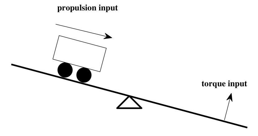
Figure 1: A vehicle, controlled by the propulsion $u_{1}$ and the torque $u_{2}$, moves on a uniform lever, where the centroid of the vehicle coincides with its center of gravity, while the pivot of the lever is at the center.

As shown in Figure 1, a vehicle, controlled by the propulsion force ${u}_{1}$ and the torque $u_{2}$, moves on a uniform lever. The centroid of the vehicle coincides with its center of gravity, while the pivot of the lever is at the center. A 4-dimensional state ${x}$ consists of the displacement from the lever’s center to the vehicle’s centroid along the lever direction, the counterclockwise deviation of the lever from the horizontal direction, and their corresponding velocities and angular velocities. In the simulation, the evolution of the state ${x}$ follows the following differential equation

$$\dot{{x}}=\begin{bmatrix}{x}_{3}\\ {x}_{4}\\ {u}_{1}/m_{1}-g\text{sin}({x}_{2})\\ 12({u}_{2}-m_{1}g\text{cos}({x}_{2}){x}_{1})/(m_{2}l^{2})\end{bmatrix}$$

where the gravitational acceleration $g$ is set to $9.8$. The mass $m_{1}$ of the vehicle is randomly generated following the uniform distribution over $[1,2]$, and the length $l$ of the lever is randomly generated following the uniform distribution over $[2,4]$, with its mass $m_{2}$ being set to the value $0.5l$.

It is stipulated that the control input ${u}$ remains constant between the sampling instants $k$ and $k+1$, determined according to the policy (2), where $A$ and $B$ are obtained by linearizing and discretizing the differential equation mentioned above. Specifically, the first-order Taylor expansion of trigonometric functions is taken around 0, with a sampling interval $0.2$ seconds.

The weight matrices $Q$ and $R$ are generated from $Q_{0},R_{0}\in\mathbb{R}^{2\times 2}$ drawn from a uniform distribution over $[0,1]$, defined as:

$$Q=\begin{bmatrix}Q_{0}Q_{0}^{\top}&\\ &0\end{bmatrix} R=R_{0}R_{0}^{\top}$$

The initial state ${x_{0}}$ and the target state $d$ are randomly selected to position the vehicle on the lever within $\pm 30$ degrees of the horizontal position.

In this simulation example, the number of trajectories is empirically set to $T=5$ and the length is set to $K=2n=8$. The zero pattern of Q is not considered during the identification process. The relative error $\|\Delta{\theta}\|/\|\theta\|$ is used for performance evaluation.

Both the baseline SDP method and the proposed method in this paper are employed for identification. Across 100 randomly generated simulation experiments, the proposed method exhibits superior efficiency and accuracy. The relative errors of both methods are depicted in Figure 2. It can be observed that the proposed method can yield more accurate IOC results with the relative errors being less than $10^{-8}$.

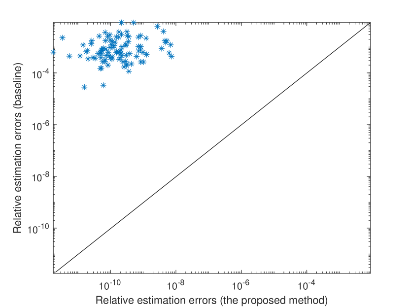
Figure 2: Scattering graph for the baseline SDP method and the proposed method in terms of the relative errors by 100 Monte-Carlo trials.

Besides, to execute 100 sets of simulation experiments, the baseline SDP method takes about 34.936 seconds, while the proposed method only takes 0.258 seconds. This notable difference in computation time stems from the proposed method’s reliance on linear estimation, while the baseline SDP method involves solving SDP optimization problems. In the simulation, the implementation of the baseline uses the Yalmip toolbox [18] and the MOSEK solver [1]. The simulation is carried out on Intel i7-8750H CPU @ 2.20GHz with 16GB RAM.

VI-C Multi-agent formation control example

The multi-agent LQT formation under fixed but unknown topology example in [32] will be tested, where the IOC problem is transformed into identifying the collective coordination patterns and intents of multi-agents, as considered in Section V. Specifically, suppose the dynamics of each agent is given by

$$\dot{{x}}_{j}={u}_{j}$$

with a control sampling interval of $0.01$ seconds. The weight matrices are taken as $Q=(L+I)\otimes I$ and $R=0.15I$, where

$$L=\begin{bmatrix}3&-1&-1&0&0&-1\\ -1&3&-1&0&-1&0\\ -1&-1&3&-1&0&0\\ 0&0&-1&1&0&0\\ 0&-1&0&0&1&0\\ -1&0&0&0&0&1\end{bmatrix}$$

and the target states $d^{j}$ are specified as follows:

$$d^{1}=\begin{bmatrix}0&0\end{bmatrix}^{\top} d^{2}=\begin{bmatrix}1&0\end{bmatrix}^{\top}\quad d^{3}=\begin{bmatrix}\frac{3}{2}&\frac{\sqrt{3}}{2}\end{bmatrix}^{\top}$$

$$d^{4}=\begin{bmatrix}1&\sqrt{3}\end{bmatrix}^{\top} d^{5}=\begin{bmatrix}0&\sqrt{3}\end{bmatrix}^{\top}\quad d^{6}=\begin{bmatrix}-\frac{1}{2}&\frac{\sqrt{3}}{2}\end{bmatrix}^{\top}$$

One typical formation trajectory is shown in Figure 3.

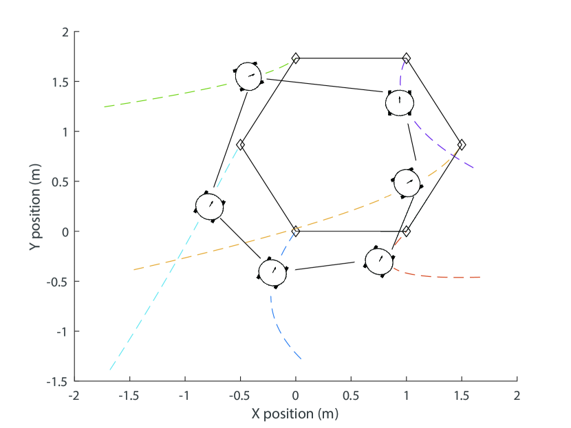
Figure 3: Trajectories of multi-agent LQT formation under a fixed topology on a two-dimensional plane.

For this simulation example, the data length is set to $K=2n$. The initial components are generated following a uniform distribution over $[-2,2]$. For each state $x_{k}$, a zero-mean normal random vector $\bar{w}_{k}$ with variance $0.1$ is added as process noise.

When only process noise exists and observation noises are absent, the number of trajectories is set to $T=n+1$. In this scenario, the relative error $\|\Delta{\theta}\|/\|\theta\|$ is less than $10^{-14}$, and the target state $d^{j}$ can be accurately recovered.

When observation noises are taken into account, the number of trajectories is set to $T=100(n+1)$, and the curve of the relative error $\|\Delta{\theta}\|/\|\theta\|$ with respect to the signal-to-noise ratio is shown in Figure 4. Figure 4 also displays its theoretical upper bound (44) against the SNR value. It can be observed that the relative estimation error is strictly smaller than the theoretical upper bound, and decays along with the SNR. This provides an experimental evidence that the proposed method can yield perfect results in the absence of observation noises.

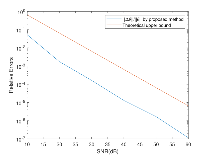
Figure 4: The variation of relative errors w.r.t. signal-to-noise ratio for $T=100$, where the blue line represents the relative error of of the proposed method, while the red line indicates its theoretical upper bound.

VII Conclusions

The inverse optimal control for a finite-horizon discrete-time LQT problem has been addressed in this paper, with the aim of jointly determining the state weight matrix, the input weight matrix and the target state according to the optimal input and state trajectories. A linearization algorithm has been proposed, which significantly outperforms the existing SDP-based methods in terms of efficiency and accuracy. In addition, theoretical guarantees have been provided for obtaining consistent estimates. Moreover, structural prior knowledge has been leveraged to reduce errors, demonstrating its potential in handling high-dimensional problems through topology identification in multi-agent systems.

One limitation of the method proposed in this paper is that it requires to observe both the optimal control input and the corresponding state trajectories. Future work might extend the current results to practical scenarios with partial state observations.

Appendix A Proof of Lemma 1

Proof:

Define the cumulative cost from the time index $k$ as

$$J_{k}=\mathbb{E}\left\{J_{k+1}+e_{k}^{\top}Qe_{k}+u_{k-1}^{\top}Ru_{k-1}\right\}$$

with $J_{K+2}=0$.

For sake of brevity, $\{u_{k},u_{k+1},\cdots,u_{K}\}$ is denoted as $u_{k:K}$ in remainder of the proof. In the following, it will be shown by induction that $\min_{u_{0:K}}J_{1}$ is reached if and only if the control input satisfies $u_{0:K}=\pi_{0:K}(Q,R,d,x_{k})$.

Let $\eta_{K+1}=q,P_{K+1}=Q$ and $\zeta_{K+1}=d^{\top}Qd$.

Firstly, with $q=-Qd$,

$$\min_{u_{K}}J_{K+1}=\min_{u_{K}}\mathbb{E}\left\{e_{K+1}^{\top}Qe_{K+1}+u_{K}^{\top}Ru_{K}\right\}$$

$$=\min_{u_{K}}\mathbb{E}\left\{x_{K+1}^{\top}Qx_{K+1}+2q^{\top}x_{K+1}+u_{K}^{\top}Ru_{K}\right\}+d^{\top}Qd$$

$$=\min_{u_{K}}\mathbb{E}\left\{x_{K+1}^{\top}P_{K+1}x_{K+1}+2\eta_{K+1}^{\top}x_{K+1}+u_{K}^{\top}Ru_{K}\right\}+\zeta_{K+1}$$

holds at $k=K$, where $\zeta_{K+1}$ is uncorrelated with $x_{K},u_{K}$.

Secondly, for any $k=0,1,\cdots,K$, if

$$\min_{u_{k:K}}J_{k+1}= \min_{u_{k}}\mathbb{E}\left\{x_{k+1}^{\top}P_{k+1}x_{k+1}+2\eta_{k+1}^{\top}x_{k+1}+u_{k}^{\top}Ru_{k}\right\}$$

$$+\zeta_{k+1}$$

holds at $k$, where $\zeta_{k+1}$ is uncorrelated with $x_{k},u_{k}$, then by substituting $x_{k+1}=Ax_{k}+Bu_{k}+w_{k}$, applying the assumptions on $w_{k}$, it can be obtained that

$$\min_{u_{k:K}}J_{k+1}= \min_{u_{k}}\left\{u_{k}^{\top}(R+B^{\top}P_{k+1}B)u_{k}\right.$$

$$\left.+2(B^{\top}P_{k+1}Ax_{k}+B^{\top}\eta_{k+1})^{\top}u_{k}\right\}$$

$$+x_{k}^{\top}A^{\top}P_{k+1}Ax_{k}+2\eta_{k+1}^{\top}Ax_{k}$$

$$+\mathbb{E}\{w_{k}^{\top}P_{k+1}w_{k}\}+\zeta_{k+1}$$

depending on a quadratic programming problem. Denote

$$\Psi_{k}(Q,R) =-(R+B^{\top}P_{k+1}B)^{-1}B^{\top}P_{k+1}A$$

$$\psi_{k}(Q,R,d) =-(R+B^{\top}P_{k+1}B)^{-1}B^{\top}\eta_{k+1}$$

then it can be obtained that

$$\min_{u_{k:K}}J_{k+1}= x_{k}^{\top}A^{\top}(P_{k+1}B\Psi_{k}+P_{k+1}A)x_{k}$$

$$+2[A^{\top}(P_{k+1}B\psi_{k}+\eta_{k+1})]^{\top}x_{k}$$

$$+\eta_{k+1}^{\top}B\psi_{k}+\mathbb{E}\{w_{k}^{\top}P_{k+1}w_{k}\}+\zeta_{k+1}$$

if and only if $u_{k}=\pi_{k}(Q,R,d,x_{k})$, where

$$\pi_{k}(Q,R,d,x_{k}) =\begin{bmatrix}\Psi_{k}(Q,R)&\psi_{k}(Q,R,d)\end{bmatrix}\begin{bmatrix}x_{k}\\ 1\end{bmatrix}$$

Moreover, let

$$\eta_{k} =q+A^{\top}(P_{k+1}B\psi_{k}+\eta_{k+1})$$

$$P_{k} =Q+A^{\top}(P_{k+1}B\Psi_{k}+P_{k+1}A)$$

$$\zeta_{k} =d^{\top}Qd+\eta_{k+1}^{\top}B\psi_{k}+\mathbb{E}\{w_{k}^{\top}P_{k+1}w_{k}\}+\zeta_{k+1}$$

it can be derived that

$$\min_{u_{k-1:K}}J_{k}= \min_{u_{k-1:K}}\mathbb{E}\left\{J_{k+1}+e_{k}^{\top}Qe_{k}+u_{k-1}^{\top}Ru_{k-1}\right\}$$

$$= \min_{u_{k-1}}\mathbb{E}\left\{x_{k}^{\top}P_{k}x_{k}+2\eta_{k}^{\top}x_{k}+u_{k-1}^{\top}Ru_{k-1}\right\}+\zeta_{k}$$

where $\zeta_{k}$ is uncorrelated with $x_{k-1},u_{k-1}$. By induction, the proof of the lemma is completed. ∎

References

• [1] Mosek ApS. Mosek optimization toolbox for matlab. User’s Guide and Reference Manual, Version, 4:1, 2019.
• [2] Kun Cao and Lihua Xie. Trust-region inverse reinforcement learning. IEEE Transactions on Automatic Control, 69(2):1037–1044, 2024.
• [3] Sheng Cao, Zhiwei Luo, and Changqin Quan. Online inverse optimal control for time-varying cost weights. Biomimetics, 9(2):84, 2024.
• [4] Sheng Cao, Zhiwei Luo, and Changqin Quan. Sequential inverse optimal control of discrete-time systems. IEEE/CAA Journal of Automatica Sinica, 11(3):1–14, 2024.
• [5] Shanelle G Clarke, Sooyung Byeon, and Inseok Hwang. A low complexity approach to model-free stochastic inverse linear quadratic control. IEEE Access, 10:9298–9308, 2022.
• [6] Wanxin Jin, Dana Kulić, Shaoshuai Mou, and Sandra Hirche. Inverse optimal control from incomplete trajectory observations. The International Journal of Robotics Research, 40(6-7):848–865, 2021.
• [7] Wanxin Jin and Shaoshuai Mou. Distributed inverse optimal control. Automatica, 129:109658, 2021.
• [8] Wanxin Jin, Todd D. Murphey, Dana Kulić, Neta Ezer, and Shaoshuai Mou. Learning from sparse demonstrations. IEEE Transactions on Robotics, 39(1):645–664, 2023.
• [9] Wanxin Jin, Todd D. Murphey, Zehui Lu, and Shaoshuai Mou. Learning from human directional corrections. IEEE Transactions on Robotics, 39(1):625–644, 2023.
• [10] Rudolf Emil Kalman. When is a linear control system optimal? 1964.
• [11] Yao Li and Chengpu Yu. Inverse stochastic optimal control for linear-quadratic tracking. In 2023 42nd Chinese Control Conference (CCC), pages 1430–1435. IEEE, 2023.
• [12] Yibei Li, Xiaoming Hu, Bo Wahlberg, and Lihua Xie. Inverse kalman filtering for systems with correlated noises. In 2023 62nd IEEE Conference on Decision and Control (CDC), pages 3626–3631, 2023.
• [13] Bosen Lian, Wenqian Xue, Frank L. Lewis, and Tianyou Chai. Inverse reinforcement learning for multi-player noncooperative apprentice games. Automatica, 145:110524, 2022.
• [14] Bosen Lian, Wenqian Xue, Frank L. Lewis, and Ali Davoudi. Inverse q-learning using input–output data. IEEE Transactions on Cybernetics, 54(2):728–738, 2024.
• [15] Bosen Lian, Wenqian Xue, Yijing Xie, Frank L. Lewis, and Ali Davoudi. Off-policy inverse q-learning for discrete-time antagonistic unknown systems. Automatica, 155:111171, 2023.
• [16] Jie Lin, Mi Wang, and Huai-Ning Wu. Composite adaptive online inverse optimal control approach to human behavior learning. Information Sciences, 638:118977, 2023.
• [17] Jin Lin, Yunjian Peng, Lei Zhang, and Jinze Li. An extended inverse reinforcement learning control for target-expert systems with different parameters. In 2023 IEEE International Symposium on Product Compliance Engineering - Asia (ISPCE-ASIA), pages 1–6, 2023.
• [18] J. Löfberg. Yalmip : A toolbox for modeling and optimization in matlab. In In Proceedings of the CACSD Conference, Taipei, Taiwan, 2004.
• [19] Jan R Magnus and Heinz Neudecker. Matrix differential calculus with applications in statistics and econometrics. John Wiley & Sons, 2019.
• [20] Marcel Menner, Peter Worsnop, and Melanie N Zeilinger. Constrained inverse optimal control with application to a human manipulation task. IEEE Transactions on Control Systems Technology, 29(2):826–834, 2019.
• [21] Timothy L Molloy, Jairo Inga Charaja, Sören Hohmann, and Tristan Perez. Inverse optimal control and inverse noncooperative dynamic game theory. Springer, 2022.
• [22] Timothy L Molloy, Jason J Ford, and Tristan Perez. Finite-horizon inverse optimal control for discrete-time nonlinear systems. Automatica, 87:442–446, 2018.
• [23] Timothy L. Molloy, Jason J. Ford, and Tristan Perez. Online inverse optimal control for control-constrained discrete-time systems on finite and infinite horizons. Automatica, 120:109109, 2020.
• [24] Anne-Sophie Puydupin-Jamin, Miles Johnson, and Timothy Bretl. A convex approach to inverse optimal control and its application to modeling human locomotion. In 2012 IEEE International Conference on Robotics and Automation, pages 531–536. IEEE, 2012.
• [25] Nikolaos Tsiantis, Eva Balsa-Canto, and Julio R Banga. Optimality and identification of dynamic models in systems biology: an inverse optimal control framework. Bioinformatics, 34(14):2433–2440, 2018.
• [26] Kevin Westermann, Jonathan Feng-Shun Lin, and Dana Kulić. Inverse optimal control with time-varying objectives: application to human jumping movement analysis. Scientific reports, 10(1):11174, 2020.
• [27] Huai-Ning Wu and Mi Wang. Distributed adaptive inverse differential game approach to leader’s behavior learning for multiple autonomous followers. IEEE Transactions on Artificial Intelligence, 4(6):1666–1678, 2023.
• [28] Huai-Ning Wu and Mi Wang. Human-in-the-loop behavior modeling via an integral concurrent adaptive inverse reinforcement learning. IEEE Transactions on Neural Networks and Learning Systems, pages 1–12, 2023.
• [29] Huai-Ning Wu and Mi Wang. Learning human behavior in shared control: Adaptive inverse differential game approach. IEEE Transactions on Cybernetics, pages 1–11, 2023.
• [30] Wenqian Xue, Patrik Kolaric, Jialu Fan, Bosen Lian, Tianyou Chai, and Frank L. Lewis. Inverse reinforcement learning in tracking control based on inverse optimal control. IEEE Transactions on Cybernetics, 52(10):10570–10581, 2022.
• [31] Wenqian Xue, Bosen Lian, Jialu Fan, Patrik Kolaric, Tianyou Chai, and Frank L. Lewis. Inverse reinforcement q-learning through expert imitation for discrete-time systems. IEEE Transactions on Neural Networks and Learning Systems, 34(5):2386–2399, 2023.
• [32] Chang-bin Yu, Yin-qiu Wang, and Jin-liang Shao. Optimization of formation for multi-agent systems based on lqr. Frontiers of Information Technology & Electronic Engineering, 17(2):96–109, 2016.
• [33] Chengpu Yu, Yao Li, Hao Fang, and Jie Chen. System identification approach for inverse optimal control of finite-horizon linear quadratic regulators. Automatica, 129:109636, 2021.
• [34] Chengpu Yu, Yao Li, Shukai Li, and Jie Chen. Inverse linear quadratic dynamic games using partial state observations. Automatica, 145:110534, 2022.
• [35] Han Zhang and Axel Ringh. Statistically consistent inverse optimal control for discrete-time indefinite linear-quadratic systems. arXiv preprint arXiv:2212.08426, 2022.
• [36] Han Zhang and Axel Ringh. Inverse linear-quadratic discrete-time finite-horizon optimal control for indistinguishable homogeneous agents: A convex optimization approach. Automatica, 148:110758, 2023.
• [37] Han Zhang and Axel Ringh. Inverse optimal control for averaged cost per stage linear quadratic regulators. Systems & Control Letters, 183:105658, 2024.
• [38] Han Zhang, Axel Ringh, Weihan Jiang, Shaoyuan Li, and Xiaoming Hu. Statistically consistent inverse optimal control for linear-quadratic tracking with random time horizon. In 2022 41st Chinese Control Conference (CCC), pages 1515–1522, 2022.
• [39] Zhenhua Zhang, Yao Li, and Chengpu Yu. Online inverse identification of noncooperative dynamic games. In 2021 IEEE International Conference on Unmanned Systems (ICUS), pages 408–413, 2021.
• [40] Mo Zhou. Valuing environmental amenities through inverse optimization: Theory and case study. Journal of Environmental Economics and Management, 83:217–230, 2017.