Stochastic Gradient Succeeds for Bandits
Abstract
We show that the stochastic gradient bandit algorithm converges to a globally optimal policy at an rate, even with a constant step size. Remarkably, global convergence of the stochastic gradient bandit algorithm has not been previously established, even though it is an old algorithm known to be applicable to bandits. The new result is achieved by establishing two novel technical findings: first, the noise of the stochastic updates in the gradient bandit algorithm satisfies a strong “growth condition” property, where the variance diminishes whenever progress becomes small, implying that additional noise control via diminishing step sizes is unnecessary; second, a form of “weak exploration” is automatically achieved through the stochastic gradient updates, since they prevent the action probabilities from decaying faster than , thus ensuring that every action is sampled infinitely often with probability . These two findings can be used to show that the stochastic gradient update is already “sufficient” for bandits in the sense that exploration versus exploitation is automatically balanced in a manner that ensures almost sure convergence to a global optimum. These novel theoretical findings are further verified by experimental results.
1 Introduction
Algorithms for multi-armed bandits (MABs) need to balance exploration and exploitation to achieve desirable performance properties (Lattimore & Szepesvári, 2020). Well known bandit algorithms generally introduce auxiliary mechanisms to control the exploration-exploitation trade-off. For example, the upper confidence bound strategies (UCB, Lai et al. (1985); Auer et al. (2002a)), manage exploration explicitly by designing auxiliary bonuses that induce optimism under uncertainty; Thompson sampling (Thompson, 1933; Agrawal & Goyal, 2012) maintains a posterior over rewards that has to be updated and sampled from tractably. The theoretical analysis of such algorithms typically focuses on bounding their regret, i.e., showing that the average reward obtained by the algorithm approaches that of the optimal action in hindsight, at a rate that is statistically optimal. However, managing exploration bonuses via uncertainty quantification is difficult in all but simple environments (Gawlikowski et al., 2021), while posterior updating and sampling can also be computationally difficult in practice, which make the UCB and Thompson sampling challenging to apply in real world scenarios.
Meanwhile, stochastic gradient-based techniques have witnessed widespread use across the breadth of machine learning. For bandit and reinforcement learning problems, stochastic gradient yields a particularly simple algorithm—the stochastic gradient bandit algorithm (Sutton & Barto, 2018, Section 2.8)—that omits any explicit control mechanism over exploration. This algorithm is naturally compatible with deep neural networks, in stark contrast to UCB and Thompson sampling, and has seen significant practical success (Schulman et al., 2015, 2017; Ouyang et al., 2022). Surprisingly, the theoretical understanding of this algorithm remains under-developed: the global convergence and regret properties of the stochastic gradient bandit algorithm is still open, which naturally raises the question:
Is the stochastic gradient bandit algorithm able to balance exploration vs. exploitation to identify an optimal action?
Such an understanding is paramount to further improving the underlying approach. In this paper, we take a step in this direction by studying the convergence properties of the canonical stochastic gradient bandit algorithm in the simplest setting of multi-armed bandits, and answer the question affirmatively: the distribution over the arms maintained by this algorithm almost surely concentrates asymptotically on a globally optimal action.
| Reference | Convergence rate | Learning rate | Remarks |
|---|---|---|---|
| Zhang et al. (2020a) | Log-barrier regularization | ||
| Ding et al. (2021) | Entropy regularization | ||
| Zhang et al. (2021) | Gradient truncation + variance reduction | ||
| Yuan et al. (2022) | ABC assumptions | ||
| Mei et al. (2022) | Oracle baseline, is initialization and problem dependent | ||
| This paper | is initialization and problem dependent | ||
Of course, the broader literature on the use of stochastic gradient techniques in reinforcement learning has a long tradition, dating back to stochastic approximation (Robbins & Monro, 1951) with likelihood ratios (“log trick”) (Glynn, 1990) and REINFORCE policy gradient estimation (Williams, 1992). It is well known that REINFORCE (Williams, 1992) with on-line Monte Carlo sampling provides an unbiased gradient estimator of bounded variance, which is sufficient to guarantee convergence to a stationary point if the learning rates are decayed appropriately (Robbins & Monro, 1951; Zhang et al., 2020b). However, convergence to a stationary point is an extremely weak guarantee for bandits, since any deterministic policy, whether optimal or sub-optimal, has a zero gradient and is therefore a stationary point. Convergence to a stationary point, on its own, is insufficient to ensure convergence to a globally optimal policy or even to establish regret bounds.
Recently, it has been shown that if true gradients are used, softmax policy gradient (PG) methods converge to a globally optimal policy asymptotically (Agarwal et al., 2021), with an rate (Mei et al., 2020b), albeit with initialization and problem dependent constants (Mei et al., 2020a; Li et al., 2021). However, these results do not apply to the gradient bandit algorithm as it uses stochastic gradients, and a key theoretical challenge is to account for the effects of stochasticity from on-policy sampling and reward noise.
More recent results on the global convergence of PG methods with stochastic updates have been established, as summarized in Table 1. In particular, Zhang et al. (2020b) showed that REINFORCE (Williams, 1992) with learning rates and log-barrier regularization has average regret. Ding et al. (2021) proved that softmax PG with learning rates and entropy regularization has sample complexity. Zhang et al. (2021) showed that with gradient truncation softmax PG gives sample complexity. Under extra assumptions, Yuan et al. (2022) obtained sample complexity with learning rates. Mei et al. (2022) analyzed on-policy natural PG with value baselines and learning rates and proved convergence rate. The results in these works are expressed in different metrics, such as average regret, sample complexity, or convergence rate, which can sometimes make comparisons difficult. However, for the bandit case, where only one example is used in each iteration, these metrics become comparable, such that sample complexity is equal to convergence rate, which is stronger than average regret, but not necessarily vice versa.111 It is worth noting that these works also contain results for general Markov decision processes (MDPs). We express their results for bandits here by treating this case as a single state MDP.
The two key shortcomings in these existing results are, first, they introduce decaying learning rates (or regularization and/or variance reduction) to explicitly control noise, and second, such auxiliary techniques generally incur additional computation and decelerate convergence to an or slower rate. The only exception to the latter is Mei et al. (2022), which considers an aggressive learning rate decay and still establishes convergence, but leverages an unrealistic baseline to achieve this.
In this paper, we provide a new global convergence analysis of stochastic gradient bandit algorithms with constant learning rates by establishing novel properties and techniques. There are two main benefits to the results presented.
-
•
By considering only constant learning rates, we show that auxiliary forms of noise control such as learning rate decay, regularization and variance reduction are unnecessary to achieve global convergence, which justifies the use of far simpler algorithms in practice.
-
•
Unlike previous work, we show that a practical and general algorithm can achieve an optimal convergence rate and regret asymptotically.
The remaining paper is organized as follows. Sections 2 and 3 introduce the gradient bandit algorithms and standard stochastic gradient analysis respectively. Section 4 presents our novel technical findings, characterizing the automatic noise cancellation effect and global landscape properties, which is then leveraged in Section 5 to establish novel global convergence results. Section 6 discusses the effect of using baselines. Section 7 presents a simulation study to verify the theoretical findings, and Section 8 provides further discussions. Section 9 briefly concludes this work.
2 Gradient Bandit Algorithms
A multi-armed bandit (MAB) problem is specified by an action set and random rewards with mean vector . For each action , the mean reward is the expectation of a bounded reward distribution,
| (1) |
where is a finite measure over , is a probability density function with respect to , and is the reward range. Since the sampled reward is bounded, we also have . We make the following assumption on .
Assumption 2.1 (True mean reward has no ties).
For all , if , then .
Remark 2.2.
2.1 is used in the proofs for Theorem 5.1. In particular, “convergence toward strict one-hot policies” above Theorem 5.1 is needed as a result of 2.1. We discuss intuition later for establishing the same result without 2.1.
According to Sutton & Barto (2018, Section 2.8), the gradient bandit algorithm maintains a softmax distribution over actions such that , where
| (2) |
and is the parameter vector to be updated.
It is obvious that Algorithm 1 is an instance of stochastic gradient ascent with an unbiased gradient estimator (Nemirovski et al., 2009), as shown below for completeness.
Proposition 2.3.
Algorithm 1 is equivalent to the following stochastic gradient ascent update on ,
| (3) | ||||
| (4) |
where , and is the Jacobian of , for all is the importance sampling (IS) estimator, and we set for all .
Based on Proposition 2.3, Sutton & Barto (2018, Section 2.8) assert that Algorithm 1 has “robust convergence properties” toward stationary points without rigorous justification. However, as mentioned in Section 1, convergence to stationary points is a very weak assertion in a MAB, since this does not guarantee sub-optimal local maxima are avoided. Hence this claim does not assure global convergence or sub-linear regret for the gradient bandit algorithm.
3 Preliminary Stochastic Gradient Analysis
In this section, we start with local convergence of stochastic gradient bandit algorithm. The understanding of the behavior of the algorithm involves assessing whether optimization progress is able to overcome the effects of the sampling noise. This trade-off reveals inability of the vanilla analysis and inspires our refined analysis.
To illustrate the basic ideas, we first recall some known results about the form of and the behavior of Algorithm 1 and make a preliminary attempt to establish convergence to a stationary point. First, is a -smooth function of (Mei et al., 2020b, Lemma 2), which implies that,
where the last equation follows from Eq. 3. Second, as is well known, the on-policy stochastic gradient is unbiased, and its variance / scale is uniformly bounded over all .
Proposition 3.1 (Unbiased stochastic gradient with bounded variance / scale).
Using Algorithm 1, we have, for all ,
where is on randomness from the on-policy sampling and reward sampling .
Therefore, according to Proposition 3.1, we have,
| (5) |
Since the goal is to maximize , we want the first term on the r.h.s. of Eq. 5 (“progress”) to overcome the second term (“noise”) to ensure that . Unfortunately, this is not achievable using a constant learning rate , since the “progress” contains a vanishing term of as while the “noise” term will remain at constant level. Therefore, based on this bound, it seems necessary to use a diminishing learning rate to control the effect of noise for local convergence. In fact, with appropriate learning rate control (Robbins & Monro, 1951; Ghadimi & Lan, 2013; Zhang et al., 2020b), it can be shown that minimum gradient norm converge to zero. From Eq. 5, by algebra and telescoping, we have,
Choosing , the r.h.s. of the above inequality is in , i.e., the minimum gradient norm approaches zero as (Ghadimi & Lan, 2013; Zhang et al., 2020b). However, the decaying learning rate will slow down the convergence as is seen. Next, we will present our novel technical characterization of the noise in stochastic gradient bandit that can allow us to avoid this choice.
4 New Analysis: Noise Vanishes Automatically
As discussed in Section 3, noise control is at the heart of standard stochastic gradient analysis, and different techniques (entropy or log-barrier regularization, learning rate schemes, momentum) are used to explicitly combat noise in stochastic updates. Here we take a different perspective by asking whether the sampling noise will automatically diminish in a way that there is no need to explicitly control it. In particular, we investigate whether the constant order of the second term in Eq. 5 (“noise”) is accurately characterizing the sampling noise, or whether this bound can be improved.
Note that the “noise” constant in Eq. 5 arises from two quantities: the standard smoothness constant of , and the variance upper bound of in Proposition 3.1. It turns out that both of these quantities can be improved.
4.1 Non-uniform Smoothness: Landscape Properties
The first key observation is a landscape property originally derived in (Mei et al., 2021b) for true policy gradient settings, which is also applicable for stochastic gradient update.
Lemma 4.1 (Non-uniform smoothness (NS), Lemma 2 in (Mei et al., 2021b)).
For all , and for all , the spectral radius of the Hessian matrix is upper bounded by , i.e., for all ,
| (6) |
It is useful to understand the intuition behind this lemma. Note that when the PG norm is small, the policy is close to a one-hot policy, and the objective has a flat local landscape; ultimately implying that the the Hessian magnitude is upper bounded by the gradient.
However, directly using Lemma 4.1 remains challenging: Consider two iterates and . Then in a Taylor expansion the PG norm of an intermediate point , , will appear, which is undesirable since is unknown. Therefore, we require an additional lemma to assert that for a sufficiently small learning rate, the PG norm of will be controlled by that of .
Lemma 4.2 (NS between iterates).
With the learning rate requirement, Lemma 4.2 is no longer only a landscape property, but also depends on updates. Using Lemma 4.2 rather than standard smoothness, in Eq. 5 can be replaced with , which implies that the “noise” is also vanishing since as . However, with simple constant upper bound of the variance of noise in Proposition 3.1, the progress term in Eq. 5 still decays faster than the noise term since . Unfortunately, this suggests that a decaying learning rate is still necessary to control the noise. Therefore, a further refined analysis of the noise variance is required.
4.2 Growth Conditions: Softmax Jacobian Behavior
Since only Lemmas 4.1 and 4.2 are still insufficient to guarantee progress without learning rate control, we need to develop a more refined variance bound of the noise that was previously unknown for gradient bandit algorithms. We first consider an example to intuitively explain why a tighter bound on the noise variance might be possible.
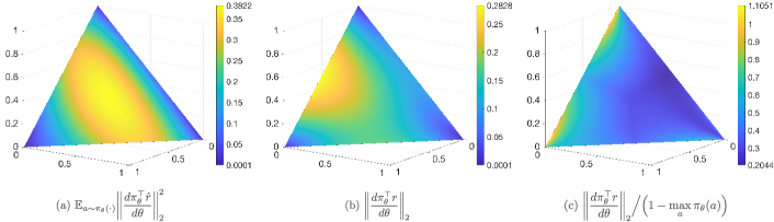
Illustration. Consider Figure 1(a), which depicts the probability simplex containing all policies over actions. Figure 1(a) shows the scale of the stochastic gradient , illustrating that when is close to any corner of the simplex, the stochastic gradient scale becomes close to . This suggests that the in Proposition 3.1 is quite loose and improvable. Figure 1(b) presents a similar visualization for the true gradient norm , demonstrating a similar behavior to the stochastic gradient scale.
We formalize this observation by proving that the stochastic gradient scale is controlled by the true gradient norm, significantly improving Proposition 3.1.
Lemma 4.3 (Strong growth condition; self-bounding noise property).
The proof sketch of Lemma 4.3 is as follows. For any , let denote the action with the largest probability, i.e.,
| (9) |
Note that characterizes how close is to any corner of the probability simplex. We first prove that,
| (10) |
which formalizes the observation in Figure 1(a). Additionally, Figure 1(c) shows that is larger than about , which suggests that the true gradient norm also characterizes a distance of from any corner of probability simplex since it has a “variance-like” structure (Eq. 14), which is formalized by proving that,
| (11) |
Combining Eqs. 10 and 11 allows one to establish Lemma 4.3, verifying the intuitive observation in Figure 1.
From this explanation, whenever the true PG norm is small and is close to a one-hot policy, the stochastic PG norm in Eq. 3 will also be small. A deeper explanation is that the softmax Jacobian is involved in the stochastic PG in Eq. 4, which cancels and annihilates the unbounded noise in reward estimator arising from the use of importance sampling.
Remark 4.4.
The “strong growth condition” was first proposed by Schmidt & Roux (2013) and later found to be satisfied in supervised learning with over-parameterized neural networks (NNs) (Allen-Zhu et al., 2019). There, given a dataset , the goal is to minimize a composite loss function,
| (12) |
Since over-parameterized NNs fit all the data points, i.e., for some , each individual loss is also since for all (e.g., squared loss and cross entropy). This guarantees that when the true gradient , the stochastic gradient for all . Hence the strong growth conditions are satisfied, and stochastic gradient descent (SGD) attains the same convergence speed as gradient descent (GD) with an over-parameterized NN (Allen-Zhu et al., 2019).
Remark 4.5.
Lemma 4.3 proves that such strong growth conditions are also satisfied in the stochastic gradient bandit algorithm, but for a different reason. For over-parameterized NNs, since the model fits every data point, zero gradient implies that the stochastic gradient is also zero. Here, in Lemma 4.3, the strong growth condition alternatively arises because of the landscape; that is, the presence of the softmax Jacobian in the stochastic gradient update annihilates the sampling noise and leads to the strong growth condition being satisfied.
4.3 No Learning Rate Decay
Finally, from Lemmas 4.2 and 4.3 we reach the result that expected progress can be guaranteed with a constant learning rate for the stochastic gradient bandit update.
Lemma 4.6 (Constant learning rates).
Using Algorithm 1 with , we have, for all ,
Lemma 4.2 indicates that is a sub-martingale. Since the reward is bounded , by Doob’s super-martingale convergence theorem we have that, almost surely, as .
Corollary 4.7.
Using Algorithm 1, we have, the sequence converges w.p. .
Therefore, from Lemmas 4.6 and 4.7 it follows that as almost surely, which implies that convergence to a stationary point is achieved without a decaying learning rate (Robbins & Monro, 1951). From Lemma 4.6, using telescoping we immediately have,
| (13) |
where . Comparing to Section 3, Eq. 13 is a stronger result of averaged gradient norm approaches zero, in terms of faster rate and constant learning rate. An interesting observation is that the average gradient convergence rate is independent with the initialization, which is different with the global convergence results in later sections. The key reason behind this outcome is that Lemmas 4.1 and 4.3 establish that the “noise” in Eq. 5 decays on the same order as the “progress” , so that a constant learning rate is sufficient for the “progress” term to overcome the “noise” term (Lemma 4.6).
5 New Global Convergence Results
Given the refined stochastic analysis from Section 4 we are now ready to establish new global convergence results for the stochastic gradient bandit in Algorithm 1.
5.1 Asymptotic Global Convergence
First, note that the true gradient norm takes the following “variance-like” expression,
| (14) |
According to as , we have that approaches a one-hot policy, i.e., for some as . Asymptotic global convergence is then proved by constructing contradictions against the assumption that the algorithm converges to a sub-optimal one-hot policy.
Theorem 5.1 (Asymptotic global convergence).
It is highly challenging to prove almost surely global convergence because (i) the iteration is a stochastic process, which it different with the true gradient settings (Agarwal et al., 2021), and (ii) the iteration is unbounded, which makes Doob’s super-martingale convergence results not applicable, unlike Corollary 4.7. The strategy and insights of Theorem 5.1 are as follows. According to Proposition 3.1, we have, for all ,
| (16) |
Now we suppose that using Algorithm 1, there exists a sub-optimal action , , such that,
| (17) |
which implies that,
| (18) |
Since , there exists a “good” action set,
| (19) |
By Eqs. 16, 18 and 19, for all large enough ,
| (20) |
which means a “good” action’s parameter is a sub-martingale. The major part of the proofs are devoted to the following key results. We have, almost surely,
| (21) | ||||
| (22) |
Eq. 21 is non-trivial since an unbounded sub-martingale is not necessarily lower bounded and could have positive probability of approaching negative infinity222Consider a random walk, , where with equal chance of . We have . However, we also have , and with positive probability, is not lower bounded., while Eq. 22 is non-trivial since the behavior of depends on different cases of how many times “good” actions are sampled as . With the above results, we have,
which is a contradiction with the assumption of Eq. 17. Therefore, the asymptotically convergent one-hot policy has to satisfy , proving Theorem 5.1. The detailed proof is provided in Section A.1.
Remark 5.2.
As mentioned in Remark 2.2, the arguments above Theorem 5.1, i.e., approaches a one-hot policy, is based on 2.1. With this result, Theorem 5.1 proves asymptotic global convergence by contradiction with the assumption of Eq. 17. In general, without 2.1, Eq. 14 approaches zero can only imply approaches a “generalized one-hot policy” (rather than a strict one-hot policy). The definition of generalized one-hot policies can be found in Eq. 147.
Remark 5.3.
It is true that Eq. 14 approaches zero is not enough for showing approaches a one-hot policy. However, Algorithm 1 is special that it is always making one action’s probability dominate others’ when there are ties. Consider with . If , then using the expected softmax PG update , we have,
which means that after one update will be even larger than . Therefore, we have,
| (23) |
for some , which implies that,
| (24) |
i.e., as . The above arguments illustrate the “self-reinforcing” nature of Algorithm 1, such that whenever two (or more) actions have the same mean reward, the update will make only one one of their probabilities larger and larger, until one eventually dominates the others as . Generalizing the arguments to stochastic updates will remove 2.1 in the proofs for Theorem 5.1.
5.2 Convergence Rate
Given Theorem 5.1, a convergence rate result can then be proved using the following inequality (Mei et al., 2020b).
Lemma 5.4 (Non-uniform Łojasiewicz (NŁ), Lemma 3 of Mei et al. (2020b)).
Assume has a unique maximizing action . Let . Then,
| (25) |
Theorem 5.5 (Convergence rate and regret).
In Theorem 5.5, the dependence on is optimal (Lai et al., 1985). However, the constant can be large, especially for a bad initialization. In short, the stochastic gradient algorithm inherits the initialization sensitivity and sub-optimal plateaus from the true policy gradient algorithm with softmax parameterization (Mei et al., 2020a). The detailed proof of Theorem 5.5 is elaborated in Section A.2.
Theorem 5.6.
There exists a problem, initialization , and a positive constant , such that, for all , we have
| (26) |
where is the reward gap of .
6 The Effect of Baselines
The original gradient bandit algorithm (Sutton & Barto, 2018) uses a baseline, which is a slightly modification of Algorithm 1. The difference is that in Algorithm 1 is replaced with , where is an action independent baseline, as shown in Algorithm 2 in Appendix B.
It is well known that action independent baselines do not introduce bias in the gradient estimate (Sutton & Barto, 2018). The utility of adding a baseline has typically been considered to be reducing the variance of the gradient estimates (Greensmith et al., 2004; Bhatnagar et al., 2007; Tucker et al., 2018; Mao et al., 2018; Wu et al., 2018). Here we show that a similar effect manifests itself through improvements in the strong growth condition.
Lemma 6.1 (Strong growth condition, Self-bounding noise property).
Note that denotes the range of after minus a baseline from sampled reward. Comparing Lemma 6.1 to Lemma 4.3 shows that the only difference is that a constant factor of is changed to . This indicates that a deeper reason for the variance reduction effect of adding a baseline is to reduce the effective reward range. The same improved constant will carry over to all the similar results, including larger constant learning rates, larger progress, and better constants in the global convergence results.
It is worth noting that the effect of baseline differs between algorithms. Here we see that without any baseline Algorithm 1 already achieves global convergence, while adding a baseline provides constant improvements. For a different natural policy gradient (NPG) method (Kakade, 2002; Agarwal et al., 2021), it is known that without using baselines, on-policy NPG can fail by converging to a sub-optimal deterministic policy (Chung et al., 2020; Mei et al., 2021a), while adding a value baseline restores a guarantee of global convergence by reducing the update aggressiveness.
7 Simulation Results
In this section, we conduct several simulations to empirically verify the theoretical findings of asymptotic global convergence and convergence rate.
7.1 Asymptotic Global Convergence
We first design experiments to justify the asymptotic global convergence. We run Algorithm 1 on stochastic bandit problems with actions. The mean reward is random generated in . For each sampled action , the observed reward is generated as , where is Gaussian noise. For the baseline in Algorithm 2, we use average reward as suggested in (Sutton & Barto, 2018), i.e., for all . The learning rate is . We use adversarial initialization, such that .
As shown in Figure 2, eventually, even if its initial value is very small, verifying the asymptotic global convergence in Theorem 5.1. On the other hand, the long plateaus observed in Figure 2 verify Theorem 5.6.
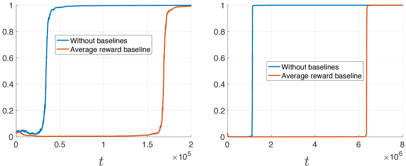
One unexpected observation in Figure 2 is that average reward baselines have worse performances, which is different with Sutton & Barto (2018). After checking numerical values, we found that since the initialization is bad, a sub-optimal action with will be pulled for most of the time, which results in . This implies that when is pulled, is increased less than without baselines, since the reward gap is also relatively small. Therefore, the average reward baseline might not be a baseline that is universally beneficial, which raises the question to design adaptive baseline, which is out of the scope of this paper, and we leave as our future work.
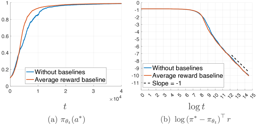
7.2 Convergence Rate
We further check the convergence rate empirically in the same problem settings. We use uniform initialization i.e., for all and the results are shown in Figure 3. Each curve is an average from independent runs, and the total iteration number is . As shown in Figure 3(b), the slope in scale is close to , which implies that . Equivalently, we have , verifying the convergence rate in Theorem 5.5.
7.3 Average Gradient Norm Convergence
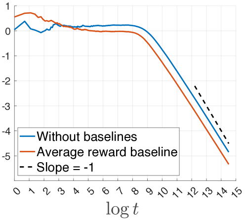
In this section, we empirically verify the finite-step convergence rate in terms of average gradient norm. We follow exactly the same experimental settings in Section 7.2, but evaluate the average gradient norm along the algorithm iterations. We illustrate the results in -scale in Figure 4. It obviously aligned well with our convergence rate in terms of average gradient norm in Eq. 13.
8 Boltzmann Exploration
The softmax parameterization used in gradient bandit algorithms is also called Boltzmann distribution (Sutton & Barto, 2018), based on which a classic algorithm EXP3 uses learning rate and achieves a rate (Auer et al., 2002b). The Botlzmann distribution has also been used in other policy gradient based algorithms. For example, Lan et al. (2022) show that mirror decent (MD) or NPG with strongly convex regularizers, increasing batch sizes and learning rates achieves a rate. The convergence in (Lan et al., 2022) heavily relies on batch observation for an accurate estimation of full gradient approximation, which is impossible in stochastic bandit setting, and thus not applicable.
There are also existing results revealing the weakness of Boltzmann distribution. Cesa-Bianchi et al. (2017) show that without count based bonuses, “Boltzmann exploration done wrong”. In particular, there exists a -armed stochastic bandit problem with rewards bounded in , when using , where
is the empirical mean estimator for , with for all , would incur linear regret . Instead of the aggressive update of parameters in softmax policy in (Cesa-Bianchi et al., 2017), the stochastic gradient bandit can be understood as a better way for parameter updates (with weights diminishing if the action is not selected) to ensure global convergence.
Cesa-Bianchi et al. (2017) also claim that the Boltzmann exploration is equivalent to the rule selecting
which is the widely used “Gumbel-Softmax” trick (Jang et al., 2016), where is a Gumbel random variable independent for all . Cesa-Bianchi et al. (2017) show a regret when replacing by , where is determined by count information . This inspires us that we may incorporate other techniques into gradient bandit algorithm and further improve it, especially for the poor initialization and problem dependent constant in Theorem 5.1 as also observed in Figure 2.
9 Conclusions
This work provides the first global convergence result for the gradient bandit algorithms (Sutton & Barto, 2018) using constant learning rates. The main technical finding is that the noise in stochastic gradient updates automatically vanishes such that noise control is unnecessary for global convergence. This work uncover a new understanding of stochastic gradient itself manages to achieve “weak exploraton” in the sense that the distribution over the arms almost surely concentrates asymptotically on a globally optimal action. One important future direction is to improve stochastic gradient to achieve “strong” exploration with finite-time optimal rates. Another direction of interest is to generalize the ideas and techniques to reinforcement learning.
Acknowledgements
The authors would like to thank anonymous reviewers for their valuable comments. Jincheng Mei would like to thank Ramki Gummadi for providing feedback on a draft of this manuscript. Csaba Szepesvári, Dale Schuurmans and Zixin Zhong gratefully acknowledge funding from the Canada CIFAR AI Chairs Program, Amii and NSERC.
References
- Agarwal et al. (2021) Agarwal, A., Kakade, S. M., Lee, J. D., and Mahajan, G. On the theory of policy gradient methods: Optimality, approximation, and distribution shift. J. Mach. Learn. Res., 22(98):1–76, 2021.
- Agrawal & Goyal (2012) Agrawal, S. and Goyal, N. Analysis of thompson sampling for the multi-armed bandit problem. In Conference on learning theory, pp. 39–1. JMLR Workshop and Conference Proceedings, 2012.
- Allen-Zhu et al. (2019) Allen-Zhu, Z., Li, Y., and Song, Z. A convergence theory for deep learning via over-parameterization. In International Conference on Machine Learning, pp. 242–252. PMLR, 2019.
- Auer et al. (2002a) Auer, P., Cesa-Bianchi, N., and Fischer, P. Finite-time analysis of the multiarmed bandit problem. Machine learning, 47(2):235–256, 2002a.
- Auer et al. (2002b) Auer, P., Cesa-Bianchi, N., Freund, Y., and Schapire, R. E. The nonstochastic multiarmed bandit problem. SIAM journal on computing, 32(1):48–77, 2002b.
- Bhatnagar et al. (2007) Bhatnagar, S., Ghavamzadeh, M., Lee, M., and Sutton, R. S. Incremental natural actor-critic algorithms. Advances in neural information processing systems, 20, 2007.
- Boucheron et al. (2009) Boucheron, S., Lugosi, G., and Massart, P. On concentration of self-bounding functions. Electronic Journal of Probability, 14:1884–1899, 2009.
- Breiman (1992) Breiman, L. Probability. SIAM, 1992.
- Cesa-bianchi & Gentile (2005) Cesa-bianchi, N. and Gentile, C. Improved risk tail bounds for on-line algorithms. In Weiss, Y., Schölkopf, B., and Platt, J. (eds.), Advances in Neural Information Processing Systems, volume 18. MIT Press, 2005. URL https://proceedings.neurips.cc/paper_files/paper/2005/file/5d75b942ab4bd730bc2e819df9c9a4b5-Paper.pdf.
- Cesa-Bianchi et al. (2017) Cesa-Bianchi, N., Gentile, C., Lugosi, G., and Neu, G. Boltzmann exploration done right. Advances in neural information processing systems, 30, 2017.
- Chung et al. (2020) Chung, W., Thomas, V., Machado, M. C., and Roux, N. L. Beyond variance reduction: Understanding the true impact of baselines on policy optimization. arXiv preprint arXiv:2008.13773, 2020.
- Ding et al. (2021) Ding, Y., Zhang, J., and Lavaei, J. Beyond exact gradients: Convergence of stochastic soft-max policy gradient methods with entropy regularization. arXiv preprint arXiv:2110.10117, 2021.
- Doob (2012) Doob, J. L. Measure theory, volume 143. Springer Science & Business Media, 2012.
- Freedman (1975) Freedman, D. A. On Tail Probabilities for Martingales. The Annals of Probability, 3(1):100 – 118, 1975. doi: 10.1214/aop/1176996452. URL https://doi.org/10.1214/aop/1176996452.
- Gawlikowski et al. (2021) Gawlikowski, J., Tassi, C. R. N., Ali, M., Lee, J., Humt, M., Feng, J., Kruspe, A., Triebel, R., Jung, P., Roscher, R., et al. A survey of uncertainty in deep neural networks. arXiv preprint arXiv:2107.03342, 2021.
- Ghadimi & Lan (2013) Ghadimi, S. and Lan, G. Stochastic first-and zeroth-order methods for nonconvex stochastic programming. SIAM Journal on Optimization, 23(4):2341–2368, 2013.
- Glynn (1990) Glynn, P. W. Likelihood ratio gradient estimation for stochastic systems. Communications of the ACM, 33(10):75–84, 1990.
- Greensmith et al. (2004) Greensmith, E., Bartlett, P. L., and Baxter, J. Variance reduction techniques for gradient estimates in reinforcement learning. Journal of Machine Learning Research, 5(9), 2004.
- Jang et al. (2016) Jang, E., Gu, S., and Poole, B. Categorical reparameterization with gumbel-softmax. arXiv preprint arXiv:1611.01144, 2016.
- Kakade (2002) Kakade, S. M. A natural policy gradient. In Advances in neural information processing systems, pp. 1531–1538, 2002.
- Lai et al. (1985) Lai, T. L., Robbins, H., et al. Asymptotically efficient adaptive allocation rules. Advances in applied mathematics, 6(1):4–22, 1985.
- Lan et al. (2022) Lan, G., Li, Y., and Zhao, T. Block policy mirror descent. arXiv preprint arXiv:2201.05756, 2022.
- Lattimore & Szepesvári (2020) Lattimore, T. and Szepesvári, C. Bandit algorithms. Cambridge University Press, 2020.
- Li et al. (2021) Li, G., Wei, Y., Chi, Y., Gu, Y., and Chen, Y. Softmax policy gradient methods can take exponential time to converge. In Conference on Learning Theory, pp. 3107–3110. PMLR, 2021.
- Mao et al. (2018) Mao, H., Venkatakrishnan, S. B., Schwarzkopf, M., and Alizadeh, M. Variance reduction for reinforcement learning in input-driven environments. arXiv preprint arXiv:1807.02264, 2018.
- McDiarmid & Reed (2006) McDiarmid, C. and Reed, B. Concentration for self-bounding functions and an inequality of talagrand. Random Structures & Algorithms, 29(4):549–557, 2006.
- Mei et al. (2020a) Mei, J., Xiao, C., Dai, B., Li, L., Szepesvári, C., and Schuurmans, D. Escaping the gravitational pull of softmax. Advances in Neural Information Processing Systems, 33:21130–21140, 2020a.
- Mei et al. (2020b) Mei, J., Xiao, C., Szepesvari, C., and Schuurmans, D. On the global convergence rates of softmax policy gradient methods. In International Conference on Machine Learning, pp. 6820–6829. PMLR, 2020b.
- Mei et al. (2021a) Mei, J., Dai, B., Xiao, C., Szepesvari, C., and Schuurmans, D. Understanding the effect of stochasticity in policy optimization. Advances in Neural Information Processing Systems, 34:19339–19351, 2021a.
- Mei et al. (2021b) Mei, J., Gao, Y., Dai, B., Szepesvari, C., and Schuurmans, D. Leveraging non-uniformity in first-order non-convex optimization. In International Conference on Machine Learning, pp. 7555–7564. PMLR, 2021b.
- Mei et al. (2022) Mei, J., Chung, W., Thomas, V., Dai, B., Szepesvari, C., and Schuurmans, D. The role of baselines in policy gradient optimization. Advances in Neural Information Processing Systems, 2022.
- Nemirovski et al. (2009) Nemirovski, A., Juditsky, A., Lan, G., and Shapiro, A. Robust stochastic approximation approach to stochastic programming. SIAM Journal on optimization, 19(4):1574–1609, 2009.
- Ouyang et al. (2022) Ouyang, L., Wu, J., Jiang, X., Almeida, D., Wainwright, C. L., Mishkin, P., Zhang, C., Agarwal, S., Slama, K., Ray, A., et al. Training language models to follow instructions with human feedback. arXiv preprint arXiv:2203.02155, 2022.
- Robbins & Monro (1951) Robbins, H. and Monro, S. A stochastic approximation method. The annals of mathematical statistics, pp. 400–407, 1951.
- Schmidt & Roux (2013) Schmidt, M. and Roux, N. L. Fast convergence of stochastic gradient descent under a strong growth condition. arXiv preprint arXiv:1308.6370, 2013.
- Schulman et al. (2015) Schulman, J., Levine, S., Abbeel, P., Jordan, M., and Moritz, P. Trust region policy optimization. In International conference on machine learning, pp. 1889–1897, 2015.
- Schulman et al. (2017) Schulman, J., Wolski, F., Dhariwal, P., Radford, A., and Klimov, O. Proximal policy optimization algorithms. arXiv preprint arXiv:1707.06347, 2017.
- Sutton & Barto (2018) Sutton, R. S. and Barto, A. G. Reinforcement Learning: An Introduction. MIT Press, 2018.
- Thompson (1933) Thompson, W. R. On the likelihood that one unknown probability exceeds another in view of the evidence of two samples. Biometrika, 25(3-4):285–294, 1933.
- Tucker et al. (2018) Tucker, G., Bhupatiraju, S., Gu, S., Turner, R., Ghahramani, Z., and Levine, S. The mirage of action-dependent baselines in reinforcement learning. In International conference on machine learning, pp. 5015–5024. PMLR, 2018.
- Williams (1992) Williams, R. J. Simple statistical gradient-following algorithms for connectionist reinforcement learning. Machine learning, 8(3):229–256, 1992.
- Wu et al. (2018) Wu, C., Rajeswaran, A., Duan, Y., Kumar, V., Bayen, A. M., Kakade, S., Mordatch, I., and Abbeel, P. Variance reduction for policy gradient with action-dependent factorized baselines. arXiv preprint arXiv:1803.07246, 2018.
- Yuan et al. (2022) Yuan, R., Gower, R. M., and Lazaric, A. A general sample complexity analysis of vanilla policy gradient. In International Conference on Artificial Intelligence and Statistics, pp. 3332–3380. PMLR, 2022.
- Zhang et al. (2020a) Zhang, J., Kim, J., O’Donoghue, B., and Boyd, S. Sample efficient reinforcement learning with reinforce. arXiv preprint arXiv:2010.11364, 2020a.
- Zhang et al. (2021) Zhang, J., Ni, C., Szepesvari, C., Wang, M., et al. On the convergence and sample efficiency of variance-reduced policy gradient method. Advances in Neural Information Processing Systems, 34:2228–2240, 2021.
- Zhang et al. (2020b) Zhang, K., Koppel, A., Zhu, H., and Basar, T. Global convergence of policy gradient methods to (almost) locally optimal policies. SIAM Journal on Control and Optimization, 58(6):3586–3612, 2020b.
Appendix A Proofs for Algorithm 1
Proposition 2.3. Algorithm 1 is equivalent to the following stochastic gradient ascent update,
| (27) | ||||
| (28) |
where , and is the Jacobian of , and for all is the importance sampling (IS) estimator, and we set for all .
Proof.
Using the definition of softmax Jacobian and , we have, for all ,
| (29) | ||||
| (30) | ||||
| (31) |
Proposition 3.1 (Unbiased stochastic gradient with bounded variance / scale). Using Algorithm 1, we have, for all ,
| (32) | ||||
| (33) |
where is on randomness from the on-policy sampling and reward sampling .
Proof.
First part, Eq. 32. For all action , the true softmax PG is,
| (34) |
For all , the stochastic softmax PG is,
| (35) | ||||
| (36) | ||||
| (37) |
For the sampled action , we have,
| (38) | ||||
| (39) | ||||
| (40) |
For any other not sampled action , we have,
| (41) | ||||
| (42) | ||||
| (43) |
Combing Eqs. 38 and 41, we have, for all ,
| (44) |
Taking expectation over , we have,
| (45) | ||||
| (46) | ||||
| (47) | ||||
| (48) |
Combining Eqs. 34 and 45, we have, for all ,
| (49) |
which implies Eq. 32 since is arbitrary.
Second part, Eq. 33. The squared stochastic PG norm is,
| (50) | ||||
| (51) | ||||
| (52) | ||||
| (53) | ||||
| (54) | ||||
| (55) |
Therefore, we have, for all , conditioning on ,
| (56) |
Taking expectation over , we have,
| (57) | ||||
| (58) | ||||
| (59) | ||||
| (60) |
Lemma 4.1 (Non-uniform smoothness (NS), Mei et al. (2021b, Lemma 2)). For all , the spectral radius of Hessian matrix is upper bounded by , i.e., for all ,
| (61) |
Proof.
See the proof in Mei et al. (2021b, Lemma 2). We include a proof for completeness.
Let be the second derivative of the map . Denote as the softmax Jacobian. By definition we have,
| (62) | ||||
| (63) | ||||
| (64) |
Continuing with our calculation fix . Then,
| (65) | ||||
| (66) | ||||
| (67) | ||||
| (68) |
where is the Kronecker’s -function defined as,
| (69) |
To show the bound on the spectral radius of , pick . Then,
| (70) | ||||
| (71) | ||||
| (72) | ||||
| (73) | ||||
| (74) | ||||
| (75) |
where is Hadamard (component-wise) product, and the last inequality uses , , , and . Therefore, we have,
| (76) | ||||
| (77) | ||||
| (78) |
Proof.
Denote with some . According to Taylor’s theorem, we have,
| (81) | ||||
| (82) |
Denote with some . We have,
| (83) | ||||
| (84) | ||||
| (85) | ||||
| (86) | ||||
| (87) |
where the second inequality is because of the Hessian is symmetric, and its operator norm is equal to its spectral radius. Therefore, we have,
| (88) | ||||
| (89) |
Denote with . Using similar calculation in Eq. 83, we have,
| (90) | ||||
| (91) |
Combining Eqs. 88 and 90, we have,
| (92) |
which, by recurring the above arguments, implies that,
| (93) |
Next, we have,
| (94) | ||||
| (95) | ||||
| (96) |
Combining Eqs. 93 and 94, we have,
| (97) | ||||
| (98) | ||||
| (99) |
Combining Eqs. 81 and 97, we have,
| (100) | ||||
| (101) |
Lemma 4.3 (Strong growth conditions / Self-bounding noise property). Using Algorithm 1, we have, for all ,
| (102) |
where .
Proof.
Given , denote as the action with largest probability, i.e., . We have,
| (103) |
According to Eq. 57, we have,
| (104) | ||||
| (105) | ||||
| (106) | ||||
| (107) | ||||
| (108) |
On the other hand, we have,
| (109) | ||||
| (110) | ||||
| (111) | ||||
| (112) | ||||
| (113) |
which implies that,
| (114) |
Using similar calculations in the proofs for Mei et al. (2021a, Lemma 2), we have,
| (115) | |||
| (116) | |||
| (117) | |||
| (118) | |||
| (119) | |||
| (120) |
which implies that,
| (121) | |||
| (122) | |||
| (123) | |||
| (124) |
where . Therefore, we have,
| (125) | ||||
| (126) | ||||
| (127) | ||||
| (128) |
Lemma 4.6 (Constant learning rates). Using Algorithm 1 with , we have, for all ,
| (129) |
Proof.
Using the learning rate,
| (130) | ||||
| (131) | ||||
| (132) | ||||
| (133) |
we have . According to Lemma 4.2, we have,
| (134) | |||
| (135) | |||
| (136) |
which implies that,
| (137) | ||||
| (138) |
where the last equation uses Algorithm 1. Taking expectation over and , we have,
| (139) | |||
| (140) | |||
| (141) | |||
| (142) | |||
| (143) |
Corollary 4.7. Using Algorithm 1, we have, the sequence converges w. p. .
Proof.
Setting , we have by Eq. 1. Define as the -algebra generated by . Note that is -measurable since is a deterministic function of . According to Lemma 4.6, using Algorithm 1, we have, for all , , which indicates that . Hence, the conditions of Doob’s super-martingale theorem (Theorem C.1) are satisfied and the result follows. ∎
A.1 Proof of Theorem 5.1
Theorem 5.1 (Asymptotic global convergence). Using Algorithm 1, we have, almost surely,
| (144) |
which implies that .
Proof.
According to Algorithm 1, for each , the update is,
| (145) |
Given , define the following set of “generalized one-hot policy”,
| (146) | ||||
| (147) |
We make the following two claims.
Claim 1.
Almost surely, approaches one “generalized one-hot policy”, i.e., there exists (a possibly random) , such that almost surely as .
Claim 2.
Almost surely, cannot approach any “sub-optimal generalized one-hot policies”, i.e., in the previous claim must be an optimal action.
From Claim 2, it follows that almost surely, as and thus the policy sequence obtained almost surely convergences to a globally optimal policy .
Proof of Claim 1. According to Corollary 4.7, we have that for some (possibly random) , almost surely,
| (148) |
Thanks to and by Lemma 4.6, we have that () satisfies the conditions of Corollary 3 in (Mei et al., 2022). Hence, by this result, almost surely,
| (149) |
which, combined with Eq. 148 also gives that almost surely. Hence,
| (150) |
According to Lemma 4.6, we have,
| (151) | ||||
| (152) |
Combining Eqs. 150 and 151, we have, with probability ,
| (153) |
which implies that, for all , almost surely,
| (154) |
We claim that , the almost sure limit of , is such that almost surely, for some (possibly random) , almost surely. We prove this by contradiction. Let . Hence, our goal is to show that . Clearly, this follows from , hence, we prove this. On , since , we also have
| (155) |
This, together with Eq. 154 gives that almost surely on ,
| (156) |
Hence, on , almost surely, for all , . This contradicts with that holds for all , and hence we must have that , finishing the proof that .
Now, let be the (possibly random) index of the action for which almost surely. Recall that contains all actions with (cf. Eq. 146). Clearly, it holds that for all ,
| (157) |
and we have, for all ,
| (158) |
which implies that,
| (159) |
Therefore, we have,
| (160) |
which means a.s. approaches the “generalized one-hot policy” in Eq. 147 as , finishing the proof of the first claim.
Proof of Claim 2. Recall that this claim stated that . The brief sketch of the proof is as follows: By Claim 1, there exists a (possibly random) such that almost surely, as . If almost surely, Claim 2 follows. Hence, it suffices to consider the event that and show that this event has zero probability mass. Hence, in the rest of the proof we assume that we are on the event when .
Since , there exists at least one “good” action such that . The two cases are as follows.
- 2a)
-
All “good” actions are sampled finitely many times as .
- 2b)
-
At least one “good” action is sampled infinitely many times as .
In both cases, we show that as (but for different reasons), which is a contradiction with the assumption of as , given that a “good” action’s parameter is almost surely lower bounded. Hence, almost surely does not happen, which means that almost surely . Let us now turn to the details of the proof. We start with some useful extra notation. For each action , for , we have the following decomposition,
| (161) |
while we also have,
| (162) |
where accounts for possible randomness in initialization of .
Define the following notations,
| (163) | ||||
| (164) | ||||
| (165) |
Recursing Eq. 161 gives,
| (166) |
Let
| (167) |
The update rule (cf. Algorithm 1) is,
| (168) |
where , and . Let be the -algebra generated by , , , , :
| (169) |
Note that are -measurable and is -measurable for all . Let denote the conditional expectation with respect to : . We have,
| (170) |
Using the above notations, we have,
| (171) | |||
| (172) | |||
| (173) |
which implies that,
| (174) | ||||
| (175) |
We also have,
| (176) |
We observe that , and,
| (177) | ||||
| (178) |
where the inequality is by . Next, we have,
| (179) | ||||
| (180) | ||||
| (181) |
and,
| (182) | ||||
| (183) | ||||
| (184) | ||||
| (185) |
Combining Eqs. 177, 179 and 182, we have,
| (186) | ||||
| (187) |
Let . Then we have, and . According to Theorem C.3, there exists event such that , and when holds,
| (188) |
which implies that,
| (189) | |||
| (190) |
where .
Recall that is the index of the (random) action with
| (191) |
As noted earlier we consider the event , where is the index of an optimal action and we will show that this event has zero probability. Since , it suffices to show that for any fixed index with , has zero probability. Hence, in what follows we fix such a suboptimal action’s index and consider the event .
Partition the action set into three parts using as follows,
| (192) | ||||
| (193) | ||||
| (194) |
Because was the index of a sub-optimal action, we have . According to Eq. 191, on , we have as because
| (195) |
Therefore, there exists such that almost surely on while we also have
| (196) |
for all , , where . Hence, for all , , , we have, , according to the definition of in Eq. 176. We have, for all , and for all ,
| (197) |
On the other hand, we have, for all , when ,
| (198) |
Hence, when holds, we have, for all ,
| (199) | ||||
| (200) | ||||
| (201) | ||||
| (202) | ||||
| (203) |
If , then is always finite and . If , we have goes to faster than , and also .
Now take any . Because as , we have that -almost surely for all there exists such that while Eq. 203 also holds for this . Take such a . By Eq. 203,
| (204) |
Hence, almost surely on ,
| (205) |
Furthermore,
| (206) |
Similarly, we can show that, almost surely on ,
| (207) |
First case. 2a). Consider the event,
| (208) |
i.e., any “good” action has finitely many updates as . Pick , such that . According to the extended Borel-Cantelli lemma (Lemma C.2), we have, almost surely,
| (209) |
Hence, taking complements, we have,
| (210) |
also holds almost surely. Next, we have,
| (211) | ||||
| (212) | ||||
| (213) | ||||
| (214) | ||||
| (215) | ||||
| (216) |
According to Eq. 209, for all . Since (from the above derivation)
| (217) |
we have that for all according to Eq. 210. Therefore, we have, , which indicates that for all , the first update in the following Eq. 218 will be conducted for infinitely many times, and the second update in Eq. 218 will be conducted for finitely many times.
| (218) |
According to 2.1, we have , and,
| (219) | ||||
| (220) |
where upper bounds the cumulative sum of the second update in Eq. 218, since every single update is bounded, and the second update in Eq. 218 is conducted for finitely many times. Hence, we have
| (221) |
Therefore, we have, for all ,
| (222) | ||||
| (223) | ||||
| (224) | ||||
| (225) | ||||
| (226) |
which is a contradiction with the assumption of Eq. 191, showing that .
Second case. 2b). Consider the complement of , where is by Eq. 208. indicates the event for at least one “good” action has infinitely many updates as .
We now show that also where .333Here, is redefined to minimize clutter; the previous definition is not used in this part of the proof. Let , and
| (227) |
Then it suffices to show that for any , , where . Hence, assume that .
Fix . Using a similar calculation to that of Eq. 203, there exists an event such that , and on , for all , for all ,
| (228) | ||||
| (229) | ||||
| (230) | ||||
| (231) |
On , , which indicates that according to Eq. 209. When , both and go to infinity while goes to infinity faster than . Hence, we have as .
Since as , with an argument parallel to that used in the previous analysis (cf. the argument after Eq. 203), we have, almost surely on ,
| (232) |
which implies that there exists such that on , we have almost surely that while we also have that for all , for all ,
| (233) |
where is from Eq. 207. For all , we have, . Note that,
| (234) |
Since , the first update in Eq. 234 will be conducted finitely many times as . On the other hand, the second update in Eq. 234 will be conducted for infinitely many times. According to and by Eq. 210, we have,
| (235) |
Recall in Eq. 207, we show that . Therefore, we have,
| (236) |
Fix any , since by Eq. 232, there exists such that when ,
| (237) | ||||
| (238) |
which implies that,
| (239) | ||||
| (240) | ||||
| (241) |
For any , we have,
| (242) | |||
| (243) | |||
| (244) | |||
| (245) |
On , we have, for , almost surely
| (246) | ||||
| (247) | ||||
| (248) | ||||
| (249) | ||||
| (250) |
Combining Eqs. 242 and 246, we have,
| (251) | ||||
| (252) | ||||
| (253) |
Therefore, by Eq. 176, on , we have, for all , for any , almost surely,
| (254) | ||||
| (255) |
According to 2.1, we have ,, and as . Therefore, there exists , such that for all , we have . Hence, when , we have,
| (256) |
Let . When , for , we have,
| (257) | ||||
| (258) | ||||
| (259) |
Hence, for , when holds (defined above Eq. 188), we have,
| (260) | ||||
| (261) | ||||
| (262) | ||||
| (263) | ||||
| (264) |
As , both and go to infinity. According to Eq. 259, we have, goes to infinity faster than . Therefore, we have .
Since as , with an argument parallel to that used in the previous analysis (cf. the argument after Eq. 203), we get that there exists a random constant , such that almost surely on , and . Denote . Then, almost surely on , and
| (265) |
According to Eq. 232, there exists , , such that almost surely on , while we also have
| (266) |
for all . Hence, on , almost surely for all ,
| (267) | ||||
| (268) | ||||
| (269) | ||||
| (270) | ||||
| (271) |
Hence, , finishing the proof. ∎
Lemma 5.4 (Non-uniform Łojasiewicz (NŁ), Mei et al. (2020b, Lemma 3)). Assume has a unique maximizing action . Let . Then,
| (272) |
Proof.
A.2 Proof of Theorem 5.5
Theorem 5.5 (Convergence rate and regret). Using Algorithm 1 with , we have, for all ,
| (275) | ||||
| (276) |
where , and is from Theorem 5.1.
Appendix B Proofs for Using Baselines
The following Algorithm 2 is same as the gradient bandit algorithm in Sutton & Barto (2018, Section 2.8).
Proposition B.1.
Algorithm 2 is equivalent to the following stochastic gradient ascent update on .
| (298) | ||||
| (299) |
where is the Jacobian of , and for all is the importance sampling (IS) estimator, and we set for all . The baseline is defined as for all .
Proof.
Using the definition of softmax Jacobian, and , we have, for all ,
| (300) | ||||
| (301) | ||||
| (302) |
Lemma B.2 (Unbiased stochastic gradient with bounded variance / scale).
Using Algorithm 2, we have, for all ,
| (303) | ||||
| (304) |
where is on randomness from the on-policy sampling and reward sampling , and is the range of reward minus baselines, i.e.,
| (305) |
Proof.
First part, Eq. 303. For all action , the true softmax PG is,
| (306) |
For all , the stochastic softmax PG is,
| (307) | ||||
| (308) | ||||
| (309) |
For the sampled action , we have,
| (310) | ||||
| (311) | ||||
| (312) |
For any other not sampled action , we have,
| (313) | ||||
| (314) | ||||
| (315) |
Combing Eqs. 310 and 313, we have, for all ,
| (316) |
Taking expectation over , we have,
| (317) | ||||
| (318) | ||||
| (319) | ||||
| (320) | ||||
| (321) |
Combining Eqs. 306 and 317, we have, for all ,
| (322) |
which implies Eq. 303 since is arbitrary.
Second part, Eq. 304. The squared stochastic PG norm is,
| (323) | ||||
| (324) | ||||
| (325) | ||||
| (326) | ||||
| (327) | ||||
| (328) |
Therefore, we have, for all , conditioning on ,
| (329) |
Taking expectation over , we have,
| (330) | ||||
| (331) | ||||
| (332) | ||||
| (333) |
Lemma B.3 (NS between iterates).
Proof.
In the proofs for Lemma 4.2, replacing with , and replacing with , we have the results. ∎
Lemma 6.1 (Strong growth conditions / Self-bounding noise property). Using Algorithm 2, we have, for all ,
| (336) |
where , and is from Eq. 305.
Proof.
Given , denote as the action with largest probability, i.e., . We have,
| (337) |
According to Eq. 330, we have,
| (338) | ||||
| (339) | ||||
| (340) | ||||
| (341) | ||||
| (342) |
Therefore, we have,
| (343) | ||||
| (344) | ||||
| (345) | ||||
| (346) |
Lemma B.4 (Constant learning rate).
Proof.
Using the learning rate,
| (348) | ||||
| (349) | ||||
| (350) | ||||
| (351) |
we have . According to Lemma B.3, we have,
| (352) | |||
| (353) | |||
| (354) |
which implies that,
| (355) | ||||
| (356) |
where the last equation uses Algorithm 2. Taking expectation over and , we have,
| (357) | |||
| (358) | |||
| (359) | |||
| (360) | |||
| (361) |
Theorem B.5.
Using Algorithm 2, we have, the sequence converges with probability one.
Proof.
As in the proof for Theorem 5.1, we set
| (362) | |||
| (363) | |||
| (364) |
which implies that,
| (365) | ||||
| (366) |
We also have,
| (367) |
In the remaining part of the proofs for Theorem 5.1, replacing with , we have the results. ∎
Appendix C Miscellaneous Extra Supporting Results
Recall that is a sub-martingale (super-martingale, martingale) if is adapted to the filtration and (, , respectively) holds almost surely for any . For brevity, let denote where the filtration should be clear from the context and we also extend this notation to such that .
Theorem C.1 (Doob’s supermartingale convergence theorem (Doob, 2012)).
If is an -adapted sequence such that and then almost surely converges (a.s.) and, in particular, a.s. as where is such that .
Lemma C.2 (Extended Borel-Cantelli Lemma, Corollary 5.29 of (Breiman, 1992)).
Let be a filtration, . Then, almost surely,
Theorem C.3.
Let be a sequence of random variables, such that for all , . Define
| (368) |
Then, for all ,
| (369) |
C.1 Proof of Theorem C.3
Proof.
Let with . We have
| (370) | |||
| (371) | |||
| (372) | |||
| (373) | |||
| (374) | |||
| (375) | |||
| (376) | |||
| (377) | |||
| (378) |
Plugging into Eq. 378, we have
| (379) |
Since for all , we have
| (380) | |||
| (381) | |||
| (382) | |||
| (383) |
Let for all , then
| (384) | |||
| (385) |
Since for all , indicating that is non-increasing with . Since , we have for all and hence is non-increasing with . Since , we have for all . Hence, we have
| (386) | |||
| (387) | |||
| (388) | |||
| (389) |
Since , we have
Lemma C.4.
Let be a sequence of random variables, such that for all , . Define the bounded martingale difference sequence and the associated martingale with conditional variance . Then, for all ,
| (390) |
LABEL:{lem:freedman_ineq} is known as Freedman’s inequality, which was originally from Freedman (1975). In detail, it is implied by Lemma 1 in Cesa-bianchi & Gentile (2005), which bounds for . For , we can apply Lemma 1 in Cesa-bianchi & Gentile (2005) with and individually to obtain Lemma C.4.
Lemma C.5.
If , then
| (391) |
Proof.
Let
| (392) |
then
| (393) | |||
| (394) | |||
| (395) | |||
| (396) |
We see that
-
•
: and increases with ;
-
•
: ;
-
•
: and decreases with .
Moreover, we have
| (397) |
Note that by assumption, we have , and then
| (398) |
Hence, when , for all , which completes the proof. ∎