Hybrid² Neural ODE Causal Modeling

Abstract

Hybrid models combine mechanistic ODE-based dynamics with flexible and expressive neural network components. Such models have grown rapidly in popularity, especially in scientific domains where such ODE-based modeling offers important interpretability and validated causal grounding (e.g., for counterfactual reasoning). The incorporation of mechanistic models also provides inductive bias in standard blackbox modeling approaches, critical when learning from small datasets or partially observed, complex systems. Unfortunately, as hybrid models become more flexible, the causal grounding provided by the mechanistic model can quickly be lost. We address this problem by leveraging another common source of domain knowledge: ranking of treatment effects for a set of interventions, even if the precise treatment effect is unknown. We encode this information in a causal loss that we combine with the standard predictive loss to arrive at a hybrid loss that biases our learning towards causally valid hybrid models. We demonstrate our ability to achieve a win-win — state-of-the-art predictive performance and causal validity — in the challenging task of modeling glucose dynamics during exercise.

1 Introduction

In many scientific and clinical domains, an influx of high resolution sensing data has brought the promise of more refined and informed scientific discovery and decision-making. The motivating example we consider in this paper is type 1 diabetes (T1D) management, where continuous glucose monitoring (CGM) and smart insulin pumps are revolutionizing care by offering near-real-time insights into physiological states (Tauschmann et al., 2022). To provide data-driven management strategies, there is a pressing need for interpretable models that not only make accurate predictions, but also grasp the causal mechanisms behind physiological responses (e.g., for counterfactual reasoning over various potential interventions). The target of causally-grounded, performant models is critical in many scientific disciplines ranging from astronomy to cell biology to neuroscience; in many of these settings, we are faced with only partial or indirect observations of a complex physiological or physical process we aim to reason about.

Blackbox sequence models have demonstrated extraordinary performance in numerous fields, including natural language processing, robotics, and demand forecasting. Popular methods include recurrent neural networks (RNNs), such as long short-term memory networks (LSTMs) (Hochreiter and Schmidhuber, 1997) and gated recurrent units (GRUs) (Chung et al., 2014); (temporal) convolutional neural networks (CNNs) (Lea et al., 2016; Bai et al., 2018; Shi et al., 2023); Transformer models, including Informer (Zhou et al., 2021) and Autoformer (Wu et al., 2021) variants; and state space sequence models such as S4 (Gu et al., 2021) and its diagonal approximation S4D (Gu et al., 2022). Despite their transformative role in many fields, the application of these models to various scientific domains has encountered challenges. An obvious hurdle is the limited size of some scientific datasets. But even in the presence of lots of data, these methods are still crippled by the incomplete nature of what can be measured. This problem is exacerbated by the fact that most data is observational: blackbox models are adept at identifying associations leading to good predictions, but may not learn causally coherent models. For example, in our T1D setting, insulin delivery frequently coincides with a planned meal or snack, which initially causes glucose to rise; so the model may incorrectly infer that insulin causes glucose to rise, when the reality is the opposite.

Sophisticated mechanistic models—specified via a set of ordinary differential equations (ODEs)—remain a preferred method in many scientific domains, as they capture lab-validated or otherwise known physical or physiological causal properties of the system. Examples include cardiac and renal modeling (Hilgemann and Noble, 1987; ten Tusscher et al., 2004; Marsh et al., 2005), immunology and viral kinetics (Perelson et al., 1996; Canini and Perelson, 2014; Passini et al., 2017), epidemiology (He et al., 2020), neural circuits (Hodgkin and Huxley, 1952; Ladenbauer et al., 2019), and pharmacokinetics (Holz and Fahr, 2001). The UVA/Padova simulator (Man et al., 2014) of insulin-glucose dynamics we consider in this paper has been FDA approved as a substitute for pre-clinical trials in the development of artificial pancreas algorithms. Of note, however, is that sophisticated mechanistic models tend to add states to capture more intricate, non-Markovian dynamics such as delays, while maintaining the tractability of linear ODEs, leading to over-parameterization, and as a result, nonidentifiability. The latest version of the UVA/Padova simulator has over 30 states. While highly parameterized, the solution space of these models fails to capture important dynamics observed in real-world data; moreover, their parameter inference is highly sensitive. Further limiting this class of models is the typical assumption of a fixed mechanistic structure with a static set of simulator parameters. In T1D, many unobserved or partially-observed time-varying factors affect glycemic responses, including stress, hormone cycles, sleep, and activity levels (cf., Wellen et al., 2005). Likewise, the causal mechanism governing glycemic responses can vary—e.g., during certain types of physical activity, multiple underlying processes (not modeled in UVA/Padova) are activated based on the available energy sources (McArdle et al., 2006).

Given these limitations, we focus on an alternative approach that hybridizes machine learning (ML) with domain knowledge encoded in mechanistic models. These hybrid models have gained traction across the natural and physical sciences (Willard et al., 2022), while being given different names and interpretations such as graybox modeling (Rico-Martinez et al., 1994), physics-informed machine learning (Karniadakis et al., 2021), universal differential equations (Rackauckas et al., 2020) and neural closure learning (Gupta and Lermusiaux, 2021). The core idea of hybrid modeling is to infuse domain inductive bias such that the trained model can gain the best of both worlds–mechanistic rigor with the flexibility and expressivity of deep learning. The hope is that hybrid methods not only allow one to solve complex modeling problems with improved precision and accuracy (Pathak et al., 2018; Willard et al., 2022), but also reduce the demand on data (Rackauckas et al., 2020), enhance reliability and robustness (Didona et al., 2015), and make the ML algorithms interpretable (Karniadakis et al., 2021; Du et al., 2019). Examples of successes of hybrid modeling in healthcare can be found in Qian et al. (2021); Sottile et al. (2021); Hussain et al. (2021).

Indeed, in Fig. 1, we see the important inductive bias such mechanistic models provide. On the one hand, the pure mechanistic model makes poor predictions due to its brittle nature while on the other hand, the flexible blackbox models are subject to overfitting. The hybrid models outperform either alternative in terms of prediction error.

Unfortunately, as we also see in Fig. 1, hybrid models can quickly lose their valid causal grounding as more and more flexible modeling components are deployed. When tasked with selecting the intervention with the largest treatment effect amongst a set of three counterfactual simulations (see Sec. 5), classification error for hybrid models gradually deteriorates as the model becomes more blackbox. Amongst the blackbox models themselves, we see that the majority of black-box models have a classification error rate above $67\%$, the error rate of random guessing.

To address these challenges, we leverage another common source of domain knowledge: rankings of various treatment effects. While domain knowledge is often insufficient to specify expected treatment effects under counterfactually-applied interventions, we are still often able to make quantitative claims about relative magnitudes of different treatment effects. For example, while we may not know the precise treatment effect of eating a small salad versus a whole birthday cake (all else held constant), we do know the sign and relative scale of treatment effect. As this prior knowledge is challenging to encode in the hybrid model itself, we introduce a causal loss function that encourages our learned model to perform well in these comparison tasks. Our hybrid loss is a convex combination of predictive loss and causal loss. When applied to training hybrid models, we refer to the overall method as hybrid² neural ODE causal modeling (H²NCM). In a real-world task of guiding individuals with T1D on the impact of interventions so they can safely exercise, we show that our H²NCMapproach achieves the best of both worlds: state-of-the-art predictive accuracy with causal validity.

Figure 1: Prediction RMSE and its standard error (left) vs. 10/50/90-th (lower/bar/upper) percentile classification error rate (right) for (1) UVA/Padova mechanistic model (UVA); (2) hybrid models: latent parameter dynamics (LP), latent parameter dynamics + state closure (LPSC), MNODE; and (3) blackbox models: neural ODE (BNODE), temporal convolutional network (TCN), LSTM, Transformer (Trans) and S4D, all trained on pure predictive loss ($\alpha=0$). The dashed gray line in the second figure corresponds to the causal classification error rate of random guessing ($2/3$).

2 The Hybrid Modeling Spectrum

In this section, we provide background on hybrid modeling. For this paper, it is useful to think of hybrid modeling as a spectrum from pure mechanistic whitebox models to fully blackbox approaches, as illustrated in Fig. 2. There are two important components to the hybrid modeling spectrum: the degree to which neural networks learn the state dynamics and the degree to which the dependencies between states encoded in the mechanistic model are maintained.

The notion of a hybrid spectrum is an oversimplification as the space of possible hybrid models involves any number of combinations of hybridizations that are not easily ordered along a single axis. However, this framework is helpful for pedagogical purposes. Further, the hybrid models we focus on in our experiments can be ordered in terms of increasing model flexibility, which helps illustrate the risk that hybrid models can lose causal validity as we walk along this spectrum (see Fig. 1).

Figure 2: Visualization of hybrid modeling spectrum for a simple mechanistic model of insulin-glucose dynamics. From left to right: (1) mechanistic model; (2) latent parameter dynamics; (3) MNODE; (4) neural ODE. Dependencies between states maintained until (4), with state dynamics increasingly flexible.

2.1 Mechanistic Models

On the far left hand side of our hybrid modeling spectrum in Fig. 2 is the pure mechanistic model specified via a set of ordinary differential equations (ODE),

$$\frac{ds}{dt}=m\bigl{(}s(t);\ \beta\bigr{)},$$ (1)

where $s$ is a vector representing the state, and $\beta$ is a vector representing the simulator parameters. In applications where interventions or other external controls represented by a vector $x$ are being applied to the observed dynamical system, we obtain a controlled ordinary differential equation (CDE),

$$\frac{ds}{dt}=m\bigl{(}s(t),x(t);\ \beta\bigr{)}.$$ (2)

For simplicity, we still refer to such systems as ODEs, just as controlled state space models are often simply called state space models. Our focus will be on this controlled setting since our interest is in causal hybrid modeling to produce (valid) counterfactual simulations for an intervention $x$. In Fig. 2, we introduce a cartoon version of such a (controlled) ODE for insulin-glucose dynamics.

2.2 Neural ODE

In the absence of mechanistic domain knowledge, neural ODEs (Rico-Martinez et al., 1992; Weinan, 2017; Haber and Ruthotto, 2017; Chen et al., 2018; Kidger, 2022) have been proposed as a blackbox approach to learning such a dynamical system:

$$\frac{ds}{dt}=f(s(t),x(t);\ \theta).$$ (3)

Here, $f$ denotes a neural network with parameters $\theta$. Neural ODEs represent the far right side of the hybrid modeling spectrum in Fig. 2. These methods have proven useful in many dynamical system modeling and simulation tasks, especially in the sciences where ODEs are a standard language for describing systems (Qian et al., 2021; Lu et al., 2021; Owoyele and Pal, 2022; Asikis et al., 2022; Li et al., 2022).

2.3 Hybrid Models

For our purposes, we introduce a general hybrid model that can be used to represent several different sub-methods:

$$\frac{ds}{dt} =c_{1}m\bigl{(}s(t),x(t);\ \beta(t)\bigr{)}+c_{2}f_{1}\bigl{(}s(t),x(t),c_{3}z(t);\ \theta\bigr{)}$$ (4)

$$\frac{dz}{dt} =f_{2}\bigl{(}x(t),z(t);\ \theta\bigr{)}$$

$$\beta(t) =\beta+c_{4}f_{3}\bigl{(}x(t),z(t);\ \theta\bigr{)}.$$

This class of hybrid models can improve upon the nominal mechanistic model in Eq. (2) by introducing (i) time-varying parameters $\beta(t)$; (ii) a flexible correction term to the mechanistic ODE given by $f_{1}$; and (iii) a time-dependent latent state vector $z(t)$. We introduce constants $c_{1},c_{2},c_{3},c_{4}\in\{0,1\}$ to “switch” between different sub-methods. If $c_{1}=1$ and $c_{2}=c_{3}=c_{4}=0$, we recover a fully mechanistic model. On the other hand, if $c_{2}=1$ and $c_{1}=c_{3}=c_{4}=0$, we obtain a blackbox neural ODE.

For other choices of these constants, we obtain various previous hybrid methods. When $c_{1}=c_{4}=1$ and $c_{2}=c_{3}=0$, we have a method that addresses infidelities of the mechanistic model solely via time-dependent parameters governed by latent dynamics $z$; we refer to this hybrid approach as latent parameter dynamics. In the context of glycemic modeling, Miller et al. (2020) use a deep state space model to capture time- and context-dependence of the simulator parameters. When $c_{1}=c_{2}=1$, we learn a flexible correction $f_{1}$ to the mechanistic model in Eq. (2). We refer to this hybrid approach as state closure. If we also have $c_{3}=1$, we learn a correction $f_{1}$ that is additionally dependent on latent states $z(t)$. If instead we have $c_{3}=c_{4}=0$, we learn a simple closure model $f_{1}$ which only depends on the mechanistic states $s(t)$ (Rico-Martinez et al., 1994).

Levine and Stuart (2022) and Karniadakis et al. (2021) provide related frameworks for defining the space of hybrid models. The above schemes, and those further described in Levine and Stuart (2022); Karniadakis et al. (2021), are not mutually exclusive and are often combined (Qian et al., 2021; Wu et al., 2022; Wang et al., 2022).

Another important component of the mechanistic model that has been ignored to this point is the set of dependencies between states encoded by the mechanistic model. To make these dependencies explicit, and to explore hybrid models that—at a dynamical modeling level—maintain the same dependencies, we introduce the notion of connectivity of the state dynamics via a set of adjacency matrices $A_{s},A_{x}$:

$$\frac{ds}{dt} =c_{1}m\bigl{(}s(t),x(t);\ A_{s},A_{x},\beta(t)\bigr{)}$$ (5)

$$\ \ +c_{2}f_{1}\bigl{(}s(t),x(t),c_{3}z(t);\ A_{s},A_{x},\theta\bigr{)}$$

$$\frac{dz}{dt} =f_{2}\bigl{(}x(t),z(t);\ \theta\bigr{)}$$

$$\beta(t) =\beta+c_{4}f_{3}\bigl{(}x(t),z(t);\ \theta\bigr{)}.$$

Here the $(i,j)$ entry of $A_{s}$ is 1 if $ds_{i}/dt$ is allowed to depend on $s_{j}(t)$, and similarly for $A_{x}$. In this way, the adjacency matrices $A_{s},A_{x}$ encode a structural equation model that constrains which state variables in $s,x$ are allowed to influence each component of $\frac{ds}{dt}$. When $c_{1}=c_{2}=1$, in contrast to the state closure model of Eq. (4), here the additive neural network correction is also forced to respect the dependencies between states.

Note that in Eq. (5), when $c_{1}=0$ but $c_{2}=1$, we maintain the dependencies between states (specified via $A_{s}$ and $A_{x}$), but allow the resulting state dynamics to be fully learned via neural networks. We refer to this model as a mechanistic neural ODE (MNODE). MNODE represents the third illustrated model in the hybrid spectrum of Fig. 2.

3 Hybrid² Modeling

Hybrid models offer significant promise in many scientific domains where ODE-based mechanistic models are commonly deployed: they can provide important inductive bias, interpretability, and causal grounding as compared to their black-box alternatives; and, compared to pure mechanistic modeling, hybrid models can reduce bias through the flexibility of neural network components. However, as one walks along the hybrid modeling spectrum—from pure mechanistic to pure blackbox—these touted advantages can quickly disappear, as illustrated in Fig. 1. In particular, there is nothing constraining a hybrid model—trained on a predictive performance objective—to maintain the causal structure and interpretability of the original mechanistic model.

We address this challenge in Sec. 3.2 by introducing a hybrid loss that mixes predictive performance with causal validity. For the latter, we again lean on domain knowledge (as we did in our use of a mechanistic model), but this time cast as knowledge about the direction of treatment effects. In other words, we presume that we know in advance that applying, e.g., $2x$ instead of $x$ to the system will increase (or decrease) the value of a target evaluation metric that depends on the observed dynamic (counterfactual) response. Encoding this information in the loss function helps us achieve a win-win of increased modeling flexibility while biasing the learning towards solutions that match our causal knowledge.

3.1 Limitations of Hybrid Models

To illustrate the potential for hybrid models to lose causal validity, take the MNODE model of Eq. (5) where $c_{1}=0$. Relying solely on the dependency graph between states while learning state dynamics can fail to distinguish parameters leading to correct directions of treatment effects. Consider data generated by a mechanistic ODE $ds/dt=-as+bx+c$, where $a,b,c$ are positive. Here the rate of change of $s$ is monotonically increasing with respect to $x$ and therefore an intervention that increases $x$ should have a positive treatment effect on $s$. However, after turning these dynamics into MNODE, we instead have $ds/dt=f(s,x;\theta);$ here, we lose the monotonicity with respect to $x$, unless a monotone neural network is intentionally used—which would severely constrain the flexibility of MNODE, the original motivation for adopting this modeling approach.

One might argue that while not explicitly encoded in the architecture, neural networks should be able to learn relatively simple signals like monotonicity from the data. Unfortunately, this is not the case when learning from noisy, observational datasets. For example, in T1D, the dosing of bolus insulin (negative effect on glucose) frequently occurs in close succession with a planned meal (positive effect). Due to the confounding effect of insulin, the hybrid model may incorrectly infer that if an individual consumes carbohydrates, glucose drops; see Fig. 3. The resulting dilemma is, while we do not want to make simplifying assumptions like linearity and monotonicity, we want to encourage our hybrid models to learn dynamics and interactions consistent with known signs of treatment effects.

Figure 3: Counterfactual simulations of 3 levels of carbohydrate intake: none (blue), 50g (orange), 100g (green), comparing MNODE trained using predictive loss ($\alpha=0$) and a hybrid loss ($\alpha=0.1$). For $\alpha=0$, MNODE incorrectly selects “none” as the intervention causing the largest resulting average blood glucose, because it incorrectly infers that carb intake decreases glucose. The model using $\alpha=0.1$ correctly selects “100g”, consistent with causally valid domain knowledge ($\mathcal{I}^{*}=\hat{\mathcal{I}}$).

3.2 The Hybrid Objective

Motivated by the preceding discussion, we encode causally relevant domain knowledge in hybrid models through the loss function itself, with the goal of biasing the learning towards causally valid models.

Preliminaries

Let $X(\mathcal{T})=\left\{x(t);t\in\mathcal{T}\right\}$ be the set of control inputs at times in $\mathcal{T}$, $\mathcal{T}\subset\mathbb{R}$. In our diabetes example, $x$ can represent interventions such as carbohydrate intake or insulin dosing for a single patient. In our preceding development, we describe models for evolution of the full state $[s(t);z(t)]$. Here we assume we have a partial observation of that state; for example, in our diabetes example, we observe glucose measurements via CGM. We denote this partial state observation by $y(t)$, and we assume without loss of generality that $y(t)=H[s(t);z(t)]$ for some projection matrix $H$ (which can be the identity matrix, $I$, if we have complete observations). We then define $Y(\mathcal{T})=\left\{y(t);t\in\mathcal{T}\right\}$ to be the corresponding set of (partial) observations over $\mathcal{T}$.

We assume we have some context window $\mathcal{T}_{\mathrm{context}}$ of controls and observations, $(X(\mathcal{T}_{\mathrm{context}}),\allowbreak Y(\mathcal{T}_{\mathrm{context}}))$. We are interested in the behavior of $y$ over a prediction window $\mathcal{T}_{\mathrm{pred}}$, represented by $Y(\mathcal{T}_{\mathrm{pred}})$, given future controls $X(\mathcal{T}_{\mathrm{pred}})$. A model $M$ takes as input $(X(\mathcal{T}_{\mathrm{context}}),Y(\mathcal{T}_{\mathrm{context}})$, $X(\mathcal{T}_{\mathrm{pred}}))$ and produces an output trajectory of $y$ over the prediction window. Below we use $M^{\dagger}$ to represent the unknown ground truth model; this is the model that generated the observations $Y(\mathcal{T}_{\mathrm{pred}})$. We use $\hat{M}$ to denote a fitted model. Throughout we use $\hat{Y}(\mathcal{T}_{\mathrm{pred}})=\left\{\hat{y}(t);t\in\mathcal{T}_{\mathrm{pred}}\right\}$ to denote our predicted output from such a fitted model.

Predictive Loss

We evaluate the predictive loss of an estimated model using mean squared error:

$$L_{\mathrm{pred}}(\hat{M})=\sum_{t\in\mathcal{T}_{\mathrm{pred}}}\Big{\|}y(t)-\hat{y}(t)\Big{\|}_{2}^{2}.$$ (6)

In practice, we have a collection of observed sequences (e.g., one per patient) and compute the loss summing over all sequences. We then normalize our loss by the total number of observed time points aggregated over the sequences.

Causal Loss

In many settings, we have a value function of our observed trajectory $u(Y(\mathcal{T}_{\mathrm{pred}}))$, that computes a meaningful scalar-valued output from a sequence input. For example, in diabetes, this value might correspond to the average glucose level over $\mathcal{T}_{\mathrm{pred}}$. For fixed context $X(\mathcal{T}_{\mathrm{context}}),Y(\mathcal{T}_{\mathrm{context}})$, we consider a range of interventions $X^{(i)}(\mathcal{T}_{\mathrm{pred}})$, $i=1,\ldots,K$, that differ from the observed $X(\mathcal{T}_{\mathrm{pred}})$. The ground truth model would produce observations $Y^{(i)}(\mathcal{T}_{\mathrm{pred}})=M^{\dagger}(X(\mathcal{T}_{\mathrm{context}}),Y(\mathcal{T}_{\mathrm{context}}),X^{(i)}(\mathcal{T}_{\mathrm{pred}}))$ for the $i$’th intervention. If we could observe these counterfactuals, then we could compute the causal effect of each intervention:

$$\tau^{(i)}=u(Y^{(i)}(\mathcal{T}_{\mathrm{pred}}))-u(Y(\mathcal{T}_{\mathrm{pred}})).$$

Domain knowledge provides valuable qualitative guidance on the direction and ordering of these treatment effects: for example, we know that holding other context constant, increasing insulin dosing should lower glucose levels, and more insulin leads to greater reductions. Unfortunately, often these causal effects cannot be precisely quantitatively estimated. For example, in managing diabetes, exact estimation of glucose levels is exceedingly challenging even in highly controlled settings.

Instead, in our causal loss, we evaluate whether the model can identify the intervention with the maximum value, rather than precise estimation of causal effects. We define:

$$\mathcal{I}^{*}=\text{argmax}_{i}\tau^{(i)}=\text{argmax}_{i}u(Y^{(i)}(\mathcal{T}_{\mathrm{pred}})).$$

In principle, we can compare this intervention to an estimated maximum value intervention under the trained model $\hat{M}$, i.e.,

$$\hat{\mathcal{I}}=\text{argmax}_{i}u(\hat{Y}^{(i)}(\mathcal{T}_{\mathrm{pred}})),$$

where $\hat{Y}^{(i)}(\mathcal{T}_{\mathrm{pred}})=\hat{M}(X(\mathcal{T}_{\mathrm{context}}),Y(\mathcal{T}_{\mathrm{context}}),$ $X^{(i)}(\mathcal{T}_{\mathrm{pred}}))$ for the $i$’th intervention.

Of course, to enable model training, we need a loss function that admits a gradient. Accordingly, rather than computing the exact maximum value intervention under the estimated model, we compute the softmax vector:

$$\hat{Q}=\sigma\Big{(}\phi u\big{(}\hat{Y}^{(1)}(\mathcal{T}_{\mathrm{pred}})\big{)}\ ,\ \ldots\ ,\ \phi u\big{(}\hat{Y}^{(K)}(\mathcal{T}_{\mathrm{pred}})\big{)}\Big{)}.$$

Here $\sigma$ is the softmax function and $\phi>0$ is a scalar “temperature” parameter: the larger $\phi$ is, the closer $\hat{Q}$ is to approximating a one-hot encoding of the true argmax. In practice we choose $\phi$ as large as possible while maintaining stable training. We compute the cross entropy (CE) loss between $\hat{Q}$ and a one-hot encoding of the true argmax $\mathcal{I}^{*}$, denoted $CE(\hat{Q},\mathcal{I}^{*})$. We refer to this as our causal loss:

$$L_{\mathrm{causal}}(\hat{M})=CE(\hat{Q},\mathcal{I}^{*}).$$ (7)

Again, in practice, we average over all observed sequences, as well as all intervention scenarios under consideration.

If one instead wants to evaluate a loss that considers the entire ranking over interventions, then we can in principle evaluate the CE loss in Eq. (7) for every possible subset of interventions. Of course, this rapidly becomes intractable with increasing $K$; in future work we plan to directly consider a loss function on the estimated ranking from $\hat{M}$.

Hybrid loss

For a given $\alpha\in[0,1]$, we define our hybrid loss as:

$$L_{\mathrm{hybrid}}(\hat{M})=(1-\alpha)L_{\mathrm{pred}}(\hat{M})+\alpha L_{\mathrm{causal}}(\hat{M}),$$ (8)

where we have overloaded notation to interpret $L_{\mathrm{pred}}$ and $L_{\mathrm{causal}}$ as the average predictive and causal losses respectively over all sequences and scenarios. Note that when $\alpha=0$, model fitting focuses entirely on prediction; when $\alpha=1$, model fitting focuses entirely on causal validity.

Model Fitting: The H²NCMApproach

A critical question in fitting hybrid ODE models is the initial condition $(s_{0}=s(t_{0}),z_{0}=z(t_{0}))$, where $t_{0}$ is the beginning of our prediction window. Two primary approaches exist for performing initial state estimation jointly with hybrid ODE parameter learning: (1) statistical state estimation methods (Chen et al., 2022; Brajard et al., 2021; Ribera et al., 2022; Levine and Stuart, 2022) and (2) blackbox encoder models (Chen et al., 2018). We take the latter approach, viewing initial state estimation through the lens of sequence-to-sequence (seq2seq) modeling.

In particular, we produce the predicted sequence $\hat{Y}(\mathcal{T}_{\mathrm{pred}})$ using $X(\mathcal{T}_{\mathrm{pred}})$ and the initial condition $(s_{0},z_{0})$ encoded from the context data $(X(\mathcal{T}_{\mathrm{context}}),Y(\mathcal{T}_{\mathrm{context}}))$. We consider a general blackbox encoder for the initial conditions:

$$(s_{0},z_{0})=M_{\mathrm{context}}\big{(}X(\mathcal{T}_{\mathrm{context}}),Y(\mathcal{T}_{\mathrm{context}});\theta_{\mathrm{context}}\big{)},$$ (9)

where $\theta_{\mathrm{context}}$ are the parameters of the encoder.

We take the decoder, $M_{\mathrm{pred}}$, to be a hybrid ODE that takes as input the initial condition $(s_{0},z_{0})$, controls $X(\mathcal{T}_{\mathrm{pred}})$, and parameters $\theta_{\mathrm{pred}}=\{\beta,\theta\}$, where $\beta$ are the simulator parameters and $\theta$ the neural network parameters. We assume the hybrid model indicator variables $c_{1},\dots,c_{4}$ and adjacency matrices $A_{s},A_{x}$ are specified. The predicted values are produced as the output of numerical integration of this hybrid ODE decoder over the window $\mathcal{T}_{\mathrm{pred}}$:

$$\hat{y}\big{(}t_{k}\big{)}=H\cdot\mbox{Integrate}(M_{\mathrm{pred}},\mathcal{T}_{\mathrm{pred}};X(\mathcal{T}_{\mathrm{pred}}),s_{0},z_{0},\theta_{\mathrm{pred}}).$$ (10)

The parameters $\theta_{\mathrm{context}}$ and $\theta_{\mathrm{pred}}$ are jointly optimized to obtain a fitted model $\hat{M}$ that minimizes the hybrid loss of Eq. (8). We refer to this approach of training such a model by optimization of hybrid loss as H²NCM.

4 Related Work

Neural Causal Models (NCMs)

NCMs use feed-forward neural networks to extend the flexibility of structural equation models (SEM) (Pearl, 1998). Note that both NCM and MNODE face the flexibility-causality dilemma in observational data settings where causal inference is challenging. Similar to the role of SEM in NCM, MNODE replaces system equations–here, dynamical systems defining mechanistic ODEs—with neural networks, while retaining the original state-connectivity graph encoding specific causal relationships. Xia et al. (2021) highlighted NCM’s limitations in treatment effect estimation without strong assumptions, while we empirically show MNODE’s inability to learn the ordering of treatment effects without causal constraints. For MNODE and related hybrid modeling approaches, we address this challenge through introducing a causal loss; in contrast, Xia et al. (2022) rely on strong distributional assumptions to maintain causality. Similarities between our work may suggest that our hybrid loss can be applied to improve causal alignment of general NCMs.

Physics-informed Neural Networks (PINNs)

PINNs, introduced by Raissi et al. (2019), use neural networks for solving partial differential equations (PDEs) by approximating solutions that conform to known differential equations. In contrast to the hybrid models of this work, PINNs: 1) typically focus on learning solutions to PDEs (rather than a governing vector field), and 2) do so via regularization in which a physics-based loss encourages the learned solution to comply with known physical laws. This method is advantageous when the system’s underlying physics are well-understood, but computationally intensive or costly to simulate directly. Related is the systems-biology-informed deep learning approach by Yazdani et al. (2020), which constrains the learned models to exhibit properties similar to pre-specified mechanistic ODEs.

Graph Network Simulator (GNS)

GNS applies the message passing architecture of graph convolution networks (GCN) to physical system simulation (Sanchez-Gonzalez et al., 2018, 2020; Pfaff et al., 2020; Wu et al., 2022; Allen et al., 2023). Poli et al. (2019) connect GNS with blackbox neural ODEs (GNODE) (see also Jin et al., 2022; Bishnoi et al., 2022; Wu et al., 2022; Allen et al., 2023; Li et al., 2022). MNODE focuses on causal relationships between features across time, rather than between spatial interactions; as such, we use directed rather than undirected graphs.

5 Experiments

5.1 Motivation: Safely Managing Exercise in T1D

Type 1 Diabetes (T1D) is an autoimmune condition characterized by the destruction of insulin producing beta-cells. To manage glucose concentrations and prevent diabetes-related complications, intensive insulin therapy through externally delivered sources (e.g., insulin pumps) is required. Regular physical activity and exercise lead to numerous health benefits such as increased insulin sensitivity, weight management, and improved psychosocial well-being. However, for individuals with T1D, due to the inability to rapidly decrease circulating insulin concentrations, exercise can also increase the risk of hypoglycemia. Despite technological advancements such as continuous glucose monitoring (CGM) and automated insulin delivery (AID) systems, individuals with T1D still face significant challenges with managing glucose concentrations around exercise. Many adults with T1D are not meeting current exercise recommendations of at least 30-minutes of moderate-to-vigorous physical activity (MVPA) per day (Riddell et al., 2017), with fear of exercise-related hypoglycemia a leading barrier (Brazeau et al., 2008). To address these challenges, there is a pressing demand for precise, reliable models that can predict individualized glycemic responses during exercise and encourage safe physical activity for all individuals with T1D.

Past efforts on modeling glycemic response to physical activity have focused on developing more intricate mechanistic models (Dalla Man et al., 2009; Liu et al., 2018; Deichmann et al., 2023), rather than devising a performant predictive model. Although glucose prediction using ML and, more recently, deep learning methods has received significant attention, a dearth of papers consider exercise periods of exercise (Oviedo et al., 2017) and the few that do do not perform well (Hobbs et al., 2019; Xie and Wang, 2020; Tyler et al., 2022). We aim to leverage hybrid modeling to predict glucose concentrations of an individual with T1D during the first 30 minutes of a planned physical activity, given historical context and expected future covariates. We chose a 30-minute prediction window because most recorded exercises in our dataset (see Sec. 5.2) last for around 30 minutes. Modeling exercise-period glucose levels is already a challenging problem and we want to distinguish this task from the (even harder) task of the post-exercise period.

5.2 Data Preparation

Our data come from the Type 1 Diabetes Exercise Initiative (T1DEXI) (Riddell et al., 2023), which can be requested via https://doi.org/10.25934/PR00008428. This is a real-world study of exercise effects on 497 adults with T1D. Participants in the study were randomly assigned to one of three types of study-specific exercise videos: aerobic, resistance, or interval for a total of six sessions over four weeks. Participants were asked to self-report their food intake and exercise habits, while their insulin dosage and relevant physiological responses were recorded by corresponding wearable devices such as insulin pumps, CGM devices, and smart watches.

We select participants on open-loop pumps, which enables real-time recording of insulin dosing with levels not proactively adjusted (and thus correlated with proximal CGM readings). We also limit our cohort to participants under 40 years old and with BMI below 30 because these participants tend to exercise more regularly and thus represent the general physically-active T1D population better.

For selected participants, we first filter out exercises shorter than 30 minutes. Then, for each exercise instance, we extract the participant’s metabolic history (basal/bolus insulin delivery, carbohydrate intake, heart rate, step count, and CGM readings) 4 hours before the start of exercise to 30 minutes after to form a 5-dimensional time series. The 4-hour context window was chosen because the effect of most bolus insulin (fast-acting insulin) lasts for around 4 hours. It is common within the T1D community to consider this time range when historical context is relevant in decision making. Finally, we filter out exercise instances with missing values. We end up with 94 exercise instances from 32 participants. See the Appendix for further data preprocessing details.

Counterfactual Simulation Sets

For each exercise instance, we form three copies to modify with one of the following sets of interventions, selected uniformly at random: (1) adding 0/50/100 grams (g) of carbohydrate at the beginning of exercise; (2) adding 0/2.5/5.0 units of insulin uniformly throughout the first 30 minutes of exercise; (3) no-change/50g carbs/10.0 units of insulin at the beginning of exercise; (4) replacing the real exercise heart rate trajectory with a prototypical trajectory seen in aerobic/resistance/interval training. These intervention sets capture the most integral pieces of well-understood and well-researched domain knowledge, allowing us to compute a reliable true ranking. In particular, increasing levels of carbohydrates progressively increase mean glucose, increasing levels of insulin progressively decrease mean glucose, and increasing exercise intensity (as measured by heart rate) leads to progressively increasing mean glucose during the short exercise period being considered (Riddell et al., 2017).

5.3 Key Implementation Details

Discretization

There are currently two mainstream methods to obtain approximate solutions to hybrid ODE variants: differentiate-then-discretize and discretize-then-differentiate (Ayed et al., 2019). We choose the latter for its simplicity and adaptability. This method approximates the hybrid ODE system with stacks of residual networks (He et al., 2016) via a forward-Euler discretization scheme

$$s_{t+1}=s_{t}+ \Delta t\big{[}c_{1}m(s_{t},x_{t};\ A_{s},A_{x},\beta_{t})$$ (11)

$$+c_{2}f_{1}(s_{t},x_{t},c_{3}z_{t};\ A_{s},A_{x},\theta)\big{]}$$

$$z_{t+1}=z_{t}+ \Delta tf_{2}(s_{t},x_{t};\ \theta)$$

$$\beta_{t+1}=\beta+ c_{4}f_{3}(x_{t+1},z_{t+1};\ \theta),$$

and then computes the gradient via backpropagation.

In the above equation we use subscript instead of parenthesis to indicate the transition from the continuous time domain to discrete time steps. In our implementation, we set $\Delta t$ to be 5 minutes, which is sampling rate of CGM readings in the T1DEXI data.

Model Reduction

Instead of the full UVA/Padova S2013 model (Man et al., 2014), which suffers from over-parameterization and redundancy, our hybrid models build upon a reduced model with the aim of reducing variance and improving generalization performance. We applied a data-driven reduction method to reduce the full UVA/Padova mechanistic model and its causal graph. See the Appendix.

Model Variants and Evaluation Procedure

We consider 3 hybrid models in the form of Eq. (5) with increasing amounts of flexibility: (1) latent parameter dynamics (LP) defined via $c_{1}=c_{4}=1,c_{2}=c_{3}=0$; (2) latent parameter dynamics plus state closure (LPSC) defined via $c_{1}=c_{2}=c_{4}=1,c_{3}=0$; and (3) mechanistic neural ODE (MNODE) defined via $c_{2}=1,c_{1}=c_{3}=c_{4}=0$. In all of these cases, the adjacency matrices $A_{s}$ and $A_{x}$ are specified based on our reduced UVA/Padova mechanistic model. We also consider the blackbox neural ODE model (BNODE) defined as in MNODE via $c_{2}=1,c_{1}=c_{3}=c_{4}=0$, but with full adjacency matrices $A_{s}=A_{x}=\mathbf{1}$ to allow arbitrary causal relationships to be learned. Finally, we provide a set of non-ODE-based blackbox sequence models: the LSTM, Transformer (Trans), temporal convolutional network (TCN), and diagonal approximation to S4 (S4D). For our mechanistic model baseline, we consider the full (not reduced) UVA-Padova S2013 simulator (UVA). We limit all models to have fewer than 25,000 parameters for fair comparison. For all of our ODE-based models, we use a multi-stack LSTM for our initial-condition encoder; the non-ODE baseline models also take the historical context as input, with model-specific encoding choices. See the Appendix for further model implementation details.

To tune our models and compute test error, due to the small dataset size, we use repeated nested cross validation with 3 repeats, 6 outer folds and 4 inner folds. The inner folds are used to tune hyperparameters and outer folds to estimate generalization error; results are averaged over three runs for which the sequences are randomly shuffled. For more details of the evaluation procedure, see the Appendix.

5.4 Results

In Fig. 4, we show prediction root mean squared error (RMSE) and classification error, calculated using the nested cross validation procedure described above, for each of the considered models as a function of $\alpha$. Here, the classification task is to correctly predict the intervention that yields the highest average glucose among a given set of 3 choices. As we vary $\alpha$, the amount we emphasize the causal loss component of our hybrid loss, we see increasing predictive RMSE for all models; however, the mechanistic and hybrid ODE models are stable across a wide range of $\alpha$ values. On the other hand, for all hybrid and blackbox models, classification error decreases with increasing $\alpha$. Note that the UVA/Padova mechanistic model does not achieve 0 classification error because the mechanistic model does not include all mechanistic components relevant to exercise. For our hybrid ODEs, we see that for $\alpha\in\{0.01,0.1\}$, we achieve very low classification error while maintaining low prediction RMSE. Thus, our hybrid loss provides a win-win for hybrid ODEs: predictive performance exceeding pure mechanistic or blackbox approaches while also having extremely low classification error, again outperforming both the mechanistic and blackbox baselines.

Recall, predicting glucose trajectories during exercise is a very challenging task. Arriving at a highly performant predictive model that also enables valid counterfactual reasoning is thus an important step towards better guiding individuals with T1D to exercise safely.

Figure 4: Predictive loss (RMSE) with its standard error and 10/50/90-th(upper/bar/lower) percentile causal classification error rate for all models, across different values of $\alpha$ (hybrid loss parameter). Within each bar group for a single model (UVA, LP, LPSC, MNODE, BNODE, TCN, LSTM, Tran, S4D), the parameter $\alpha$ increases from left to right as color changes from dark to light, taking the values $\{0,1\mathrm{e}{-4},1\mathrm{e}{-3},1\mathrm{e}{-2},1\mathrm{e}{-1},1\}$ successively. The dashed line in the bottom figure corresponds to the causal classification error of random guessing ($2/3$).

6 Discussion

We presented H²NCM, a method for integrating domain knowledge not only through a hybrid model, but also through a hybrid loss that encourages causal validity. Our experiments in the challenging real-world setting of predicting glucose responses during exercise in individuals with T1D demonstrate the importance of our H²NCMapproach. We see a win-win where—across a wide range of settings of $\alpha$—our state-of-the-art predictive performance does not drop while the causal validity dramatically improves. In theory, models that can do both tasks well should align better with the true underlying system $M^{\dagger}$ and thus generalize better to unseen data, especially in the presence of distribution shifts, noise, and incompleteness, all frequent situations in health datasets. Our proposed hybrid loss may aid other modeling frameworks as well, an area of future exploration.

7 Acknowledgements

This work was supported in part by AFOSR Grant FA9550-21-1-0397, ONR Grant N00014-22-1-2110, NSF Grant 2205084, the Stanford Institute for Human-Centered Artificial Intelligence (HAI), the Helmsley Charitable Trust, and the Eric and Wendy Schmidt Center at the Broad Institute of MIT and Harvard. EBF is a Chan Zuckerberg Biohub – San Francisco Investigator. This publication is based on research using data from Jaeb Center for Health Research Foundation that has been made available through Vivli, Inc. Vivli has not contributed to or approved, and is not in any way responsible for, the contents of this publication.

Appendix A UVA-Padova Simulator S2013

Here we provide the exact full UVA-Padova S2013 model equations. Variables that are not given meaningful interpretations are model parameters.

A.1 Summary Diagram

At a high level, UVA-Padova can be summarized by the diagram in Figure 5, which is taken from Figure 1 in Man et al. (2014). It divides the complex physiological system into 10 subsystems, which are linked by key causal states such as Rate of Appearance, Endogenous Glucose Production and Utilization. Next, we will introduce each subsystem one by one and also explain the physiological meanings behind state variables.

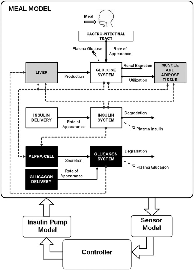
Figure 5: UVA/Padova Simulator S2013, taken from Figure 1 of Man et al. (2014)

A.2 Glucose Subsystem

$$\dot{G}_{p}=EGP+Ra-U_{ii}-E-k_{1}G_{p}+k_{2}G_{t}$$ (12)

$$\dot{G}_{t}=-U_{id}+k_{1}G_{p}-k_{2}G_{t}$$ (13)

$$G=G_{p}/V_{G}$$ (14)

$G_{p}$: Plasma Glucose, $G_{t}$ Tissue Glucose, $EGP$: Endogenous Glucose Production Rate, $Ra$ Rate of Glucose Appearance, $U_{ii}$: Insulin-independent Utilization Rate, $U_{id}$: Insulin-dependent Utilization Rate, $E$ Excretion Rate, $V_{G}$ Volume Parameter, $G$ Plasma Glucose Concentration

A.3 Insulin Subsystem

$$\dot{I}_{p}=-(m_{2}+m_{4})I_{p}+m_{1}I_{l}+Rai$$ (15)

$$\dot{I}_{t}=-(m_{1}+m_{3})I_{t}+m_{2}I_{p}$$ (16)

$$I=I_{p}/V_{I}$$ (17)

$I_{p}$ Plasma Insulin, $I_{l}$ Liver Insulin, $Rai$ Rate of Insulin Appearance, $V_{l}$ Volume Parameter, $I$ Plasma Insulin Concentration

A.4 Glucose Rate of Appearance

$$Q_{sto}=Q_{sto1}+Q_{sto2}$$ (18)

$$\dot{Q}_{sto1}=-k_{gri}Q_{sto1}+D\cdot\delta$$ (19)

$$\dot{Q}_{sto2}=-k_{empt}(Q_{sto})\cdot Q_{sto2}+k_{gri}Q_{sto1}$$ (20)

$$\dot{Q}_{gut}=-k_{abs}Q_{gut}+k_{empt}(Q_{sto})\cdot Q_{sto2}$$ (21)

$$Ra=fk_{abs}Q_{gut}/(BW)$$ (22)

$$k_{empt}(Q_{sto})=k_{min}+(k_{max}-k_{min})(\tanh{}(\alpha Q_{sto}-\alpha bD)-\tanh{}(\beta Q_{sto}-\beta cD)+2)/2$$ (23)

$Q_{sto1}$: First Stomach Compartment, $Q_{sto2}$: Second Stomach Compartment, $Q_{gut}$: Gut Compartment, $\delta$ Carbohydrate Ingestion Rate

A.5 Endogenous Glucose Production

$$EGP=k_{p1}-k_{p2}G_{p}-k_{p3}X^{L}+\xi X^{H}$$ (24)

$$\dot{X}^{L}=-k_{i}(X^{L}-I_{r}]$$ (25)

$$\dot{I}_{r}=-k_{i}(I_{r}-I)$$ (26)

$$\dot{X}^{H}=-k_{H}X^{H}+k_{H}\max(H-H_{b})$$ (27)

$X^{L}$: Remote Insulin Action on EGP, $X^{H}$: Glucagon Action on EGP, $I_{r}$ Remote Insulin Concentration, $H$ Plasma Glucagon Concentration, $H_{b}$: Basal Glucagon Concentration Parameter

A.6 Glucose Utilization

$$U_{ii}=F_{cns}$$ (28)

$$U_{id}=\frac{(V_{m0}+V_{mx}X(1+r_{1}\cdot risk))G_{t}}{K_{m0}+G_{t}}$$ (29)

$$\dot{X}=-p_{2U}X+p_{2U}(I-I_{b})$$ (30)

$$risk=\begin{cases}0&G_{b}\leq G\\ 10(\log(G)-\log(G_{b}))^{2r_{2}}&G_{th}\leq G<G_{b}\\ 10(\log(G_{th})-\log(G_{b}))^{2r_{2}}&G<G_{th}\\ \end{cases}$$ (31)

$F_{cns}$: Glucose Independent Utilization Constant, $X$: Insulin Action on Glucose Utilization, $I_{b}$ Basal Insulin Concentration Constant, $risk$ Hypoglycemia Risk Factor, $G_{b}$ Basal Glucose Concentration Parameter, $G_{th}$ Hypoglycemia Glucose Concentration Threshold.

A.7 Renal Excretion

$$\dot{E}=k_{e1}\max(G_{p}-k_{e2},0)$$ (32)

A.8 Subcutaneous Insulin Kinetics

$$Rai=k_{a1}I_{sc1}+k_{a2}I_{sc2}$$ (33)

$$\dot{I}_{sc1}=-(k_{d}+k_{a1})I_{sc1}+IIR$$ (34)

$$\dot{I}_{sc2}=k_{d}I_{sc1}-k_{a2}I_{sc2}$$ (35)

$I_{sc1}$: First Subcutaneous Insulin Compartment, $I_{sc2}$: Second Subcutaneous Insulin Compartment, $IIR$ Exogenous Insulin Delivery Rate

A.9 Subcutaneous Glucose Kinetics

$$\dot{G}_{s}=-T_{s}G_{s}+T_{s}G$$ (36)

$G_{s}$: Subcutaneous Glucose Concentration

A.10 Glucagon Secretion and Kinetics

$$\dot{H}=-nH+SR_{H}+Ra_{H}$$ (37)

$$SR_{H}=SR^{s}_{H}+SR^{d}_{H}$$ (38)

$$\dot{SR}^{s}_{H}=\begin{cases}-\rho\left[SR_{H}^{s}-\max\left(\sigma_{2}(G_{th}-G)+SR_{H}^{b},0\right)\right]&\quad G\geq G_{b}\\ -\rho\left[SR_{H}^{s}-\max\left(\frac{\sigma(G_{th}-G)}{I+1}+SR_{H}^{b},0\right)\right]&\quad G<G_{b}\end{cases}$$ (39)

$$\dot{SR}^{d}_{H}=\eta\max(-\dot{G},0)$$ (40)

$SR_{H}^{s}$: First Glucagon Secretion Compartment, $SR_{H}^{d}$: Second Glucagon Secretion Compartment, $SR_{H}^{b}$: Basal Glucagon Secretion Parameter, $Ra_{H}$: Rate of Glucagon Appearance

A.11 Subcutaneous Glucagon Kinetics

$$\dot{H}_{sc1}=-(k_{h1}+k_{h2})H_{sc1}+H_{inf}$$ (41)

$$\dot{H}_{sc2}=k_{h1}H_{sc1}-k_{h3}H_{sc2}$$ (42)

$$Ra_{H}=k_{h3}H_{sc2}$$ (43)

$H_{sc1}$: First Subcutaneous Glucagon Compartment, $H_{sc2}$: Second Subcutaneous Glucagon Compartment, $H_{inf}$ Subcutaneous Glucagon Infusion Rate.

Appendix B Reduced UVA-Padova for DTDSim2

We used the a reduced version of UVA-Padova S2013 in the implementation of Latent Parameter Model and Latent Parameter with State Closure Model. It comprises the following equations:

$$\dot{G}_{p}=EGP+Ra-U_{ii}-E-k_{1}G_{p}+k_{2}G_{t}$$ (44)

$$\dot{G}_{t}=-U_{id}+k_{1}G_{p}-k_{2}G_{t}$$ (45)

$$\dot{I}_{p}=-(m_{2}+m_{4})I_{p}+m_{1}I_{l}+IIR$$ (46)

$$\dot{I}_{t}=-(m_{1}+m_{3})I_{t}+m_{2}I_{p}$$ (47)

$$Q_{sto}=Q_{sto1}+Q_{sto2}$$ (48)

$$\dot{Q}_{sto1}=-k_{gri}Q_{sto1}+D\cdot\delta$$ (49)

$$\dot{Q}_{sto2}=-k_{empt}(Q_{sto})\cdot Q_{sto2}+k_{gri}Q_{sto1}$$ (50)

$$\dot{Q}_{gut}=-k_{abs}Q_{gut}+k_{empt}(Q_{sto})\cdot Q_{sto2}$$ (51)

$$Ra=fk_{abs}Q_{gut}/(BW)$$ (52)

$$k_{empt}(Q_{sto})=k_{min}+(k_{max}-k_{min})(\tanh{}(\alpha Q_{sto}-\alpha bD)-\tanh{}(\beta Q_{sto}-\beta cD)+2)/2$$ (53)

$$EGP=k_{p1}-k_{p2}G_{p}-k_{p3}X^{L}$$ (54)

$$\dot{X}^{L}=-k_{i}(X^{L}-I_{p})$$ (55)

$$U_{ii}=F_{cns}$$ (56)

$$U_{id}=\frac{(V_{m0}+V_{mx}X)G_{t}}{K_{m0}+G_{t}}$$ (57)

$$\dot{X}=-p_{2U}X+p_{2U}I_{p}$$ (58)

Comparing to the full model, we performed the following:

1. We replaced states $G,I$ with $G_{p},I_{p}$ as they only differ by a constant.

2. We removed the whole glucagon system to reduce model variance because most T1D patients do not have exogenous glucagon delivery, and their body’s own glucagon regulation system is often impaired, a common symptom of T1D (Bisgaard Bengtsen and Møller, 2021).

3. We removed the renal excretion system, as renal excretion of glucose only takes place during episodes of severe hyperglycemia, which does not happen very often to patients on insulin pumps.

4. We removed the subcutaneous glucose/insulin kinetics systems/the remote insulin state they are solely meant to introduce delays, which already exist in the data (CGM readings are only taken every 5 minutes).

5. We removed the hypoglycemia risk factor $risk$ as it is used to model a relatively uncommon phenomenon.

We verified these reduction changes on a validation set that was taken out of the training set to make sure they do not break our models.

Appendix C MNODE Graph Reduction Heuristic

We start with the full UVA/Padova causal graph as shown in Figure 6, this graph is obtained by adding the physical activity model graph from Dalla Man et al. (2009) to the UVA/Padova S2013 (Man et al., 2014) causal graph. Note that in the illustration, the node HR actually refers to both heart rate and step count, as we consider these two features both crucial indicators of physical activity intensity.

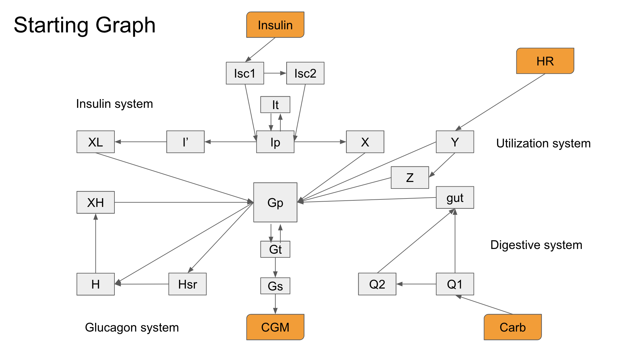
Figure 6: The Starting Graph for MNODE Graph Reduction Heuristic

1. Step 1: For each Strongly Connected Component in the graph (indicated in Figure 7(a)), try collapsing it into a single node and evaluate MNODE’s performance with the resulting graph on the validation set. Adopt the change that (1) has the least loss among all trials and (2) has loss that is within 10 percent increase of the best loss ever achieved so far. The second condition is to make sure we are not picking among a set of bad choices and at the same time to encourage exploration (i.e. can proceed as long as loss does not increase too much). The metric we use is the hybrid loss with $\alpha=0.6$ (we picked an $\alpha$ that is not used in the actual experiments to avoid bias).

2. Step 2: Repeat step 1 until no change satisfy both criteria. Figure 7 shows an illustrative summary of step 1 and step 2.

   

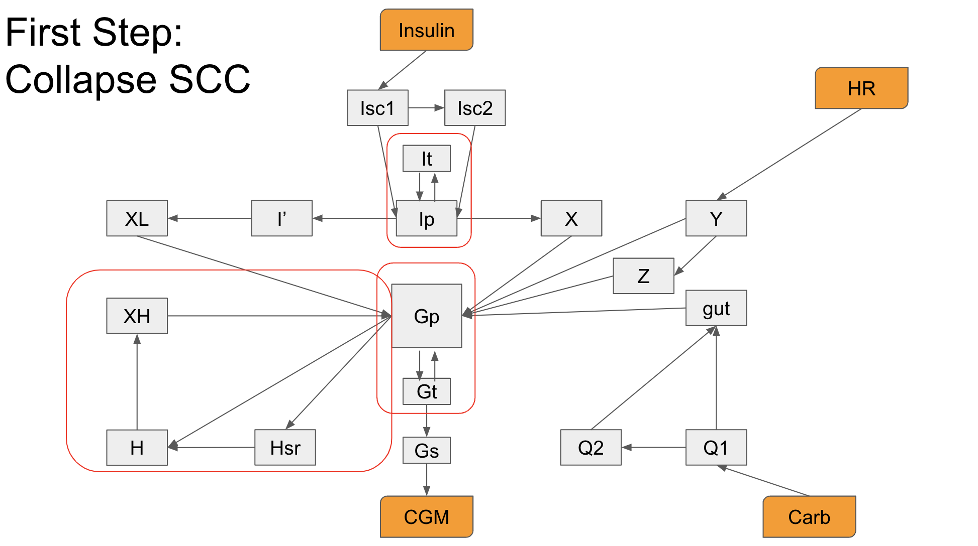
   (a) SCCs in the Starting Graph

   

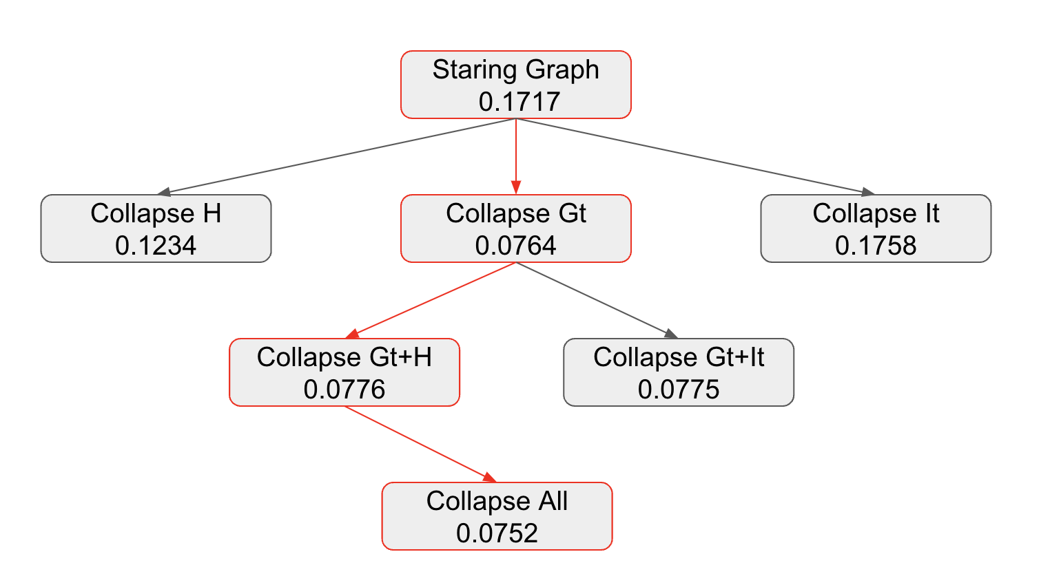
   (b) Reduction Tree of the SCCs

   

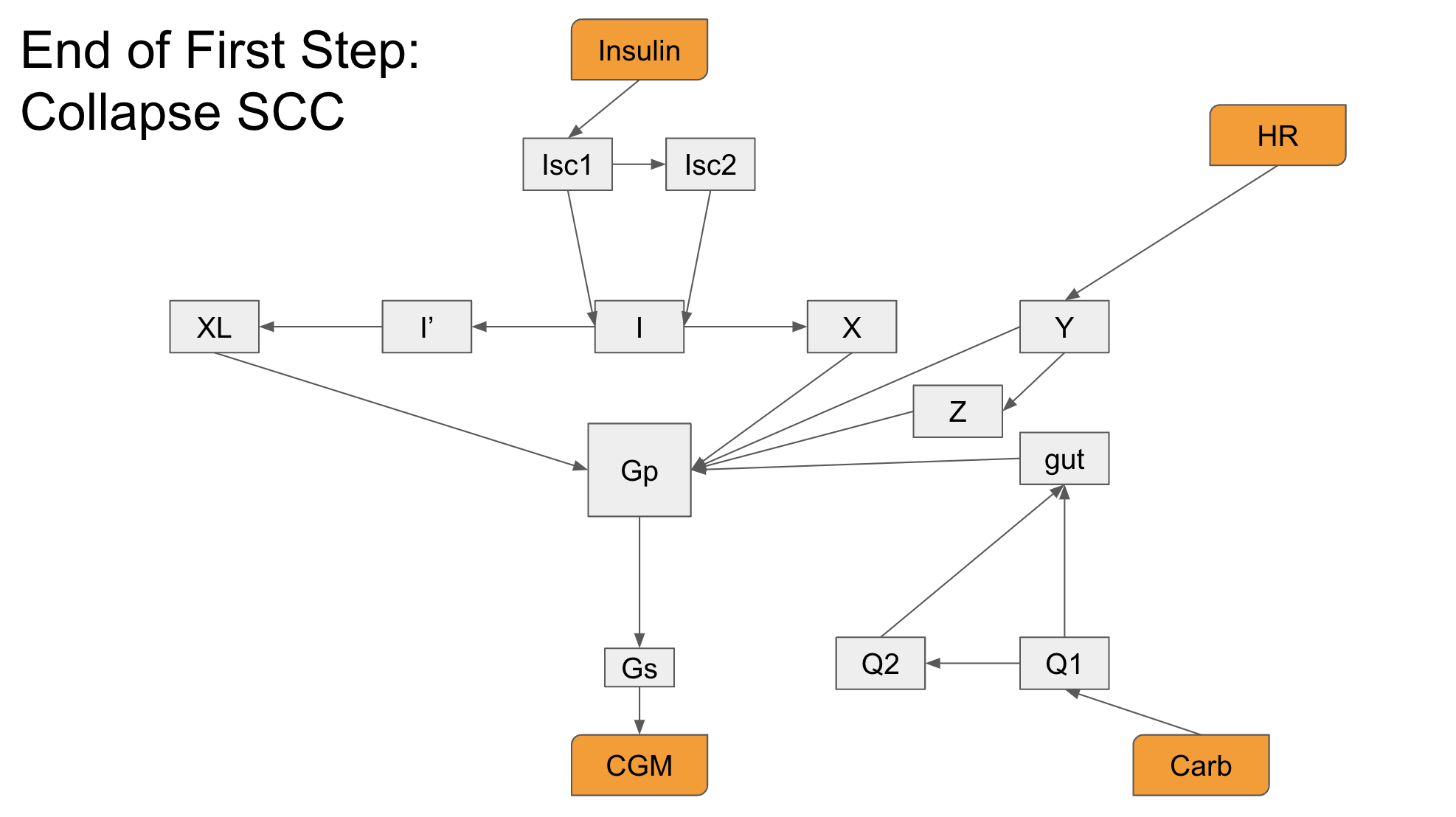
   (c) End Graph of the SCC Step

   Figure 7: Illustration of the Collapsing SCC Step of Our Heuristic

3. Step 3: For each group of non-overlapping paths with same source and destination nodes, try merge them by keeping only the path of greatest length and evaluate MNODE’s performance with the resulting graph on the validation set. Adopt the change with the same criteria as in step 1.

4. Step 4: Repeat step 3 until no change satisfy both criteria. Figure Figure 8 shows an illustrative summary of step 3 and step 4.

   

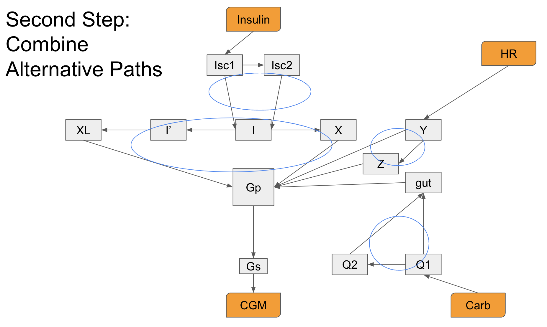
   (a) Non-overlapping Path Groups in the Starting Graph

   

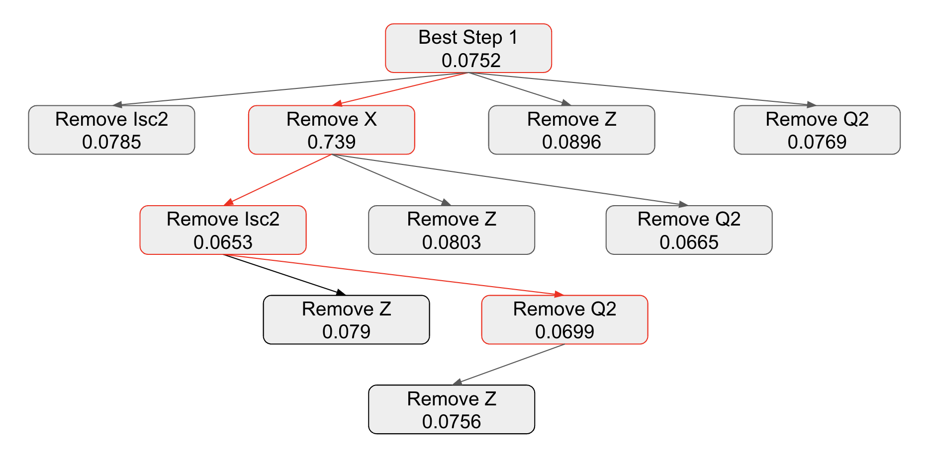
   (b) Reduction Tree of the Non-overlapping Paths

   

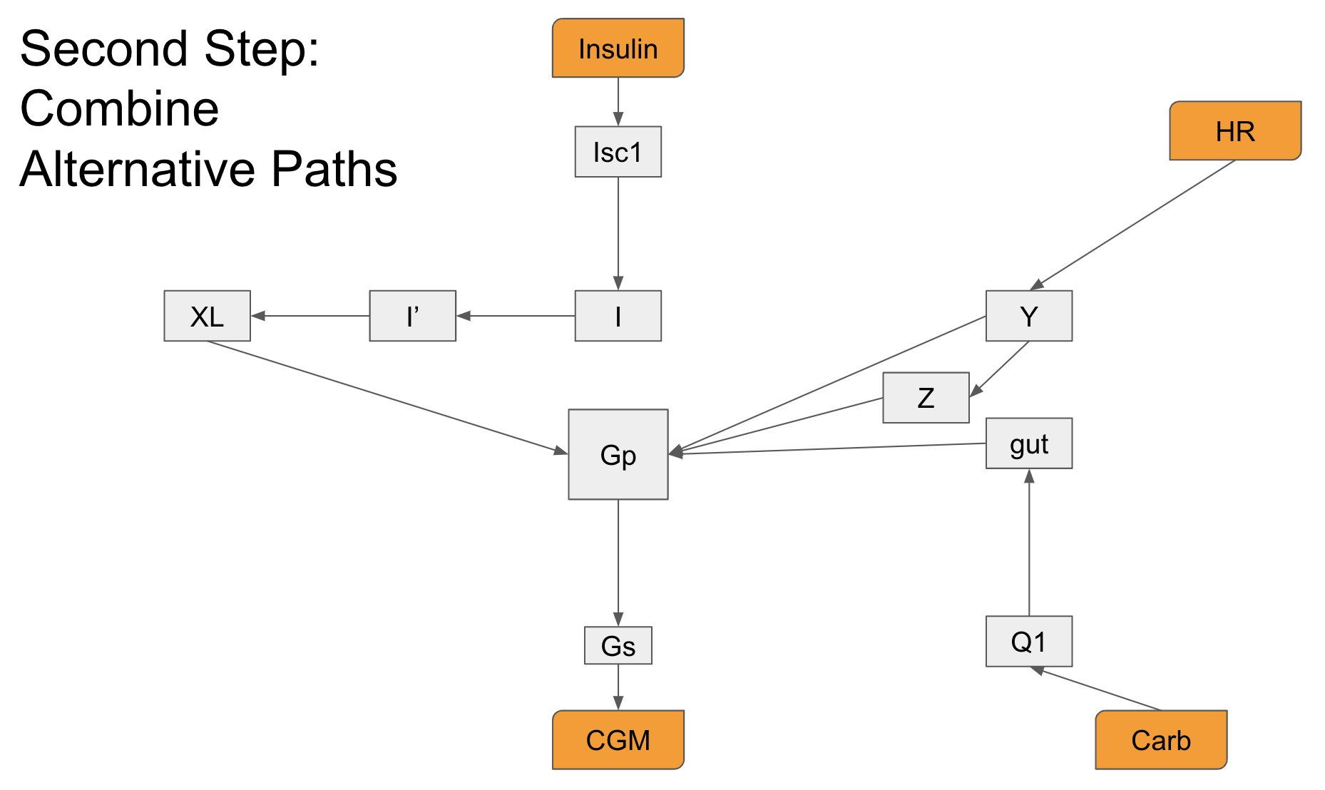
   (c) End Graph of the Path Combine Step

   Figure 8: Illustration of the Combining Non-overlapping Paths Step of Our Heuristic

5. Step 5: For each path between an input node and the output node (at this point they should all be disjoint), try reducing its length by 1 via removing one intermediate node and evaluate MNODE’s performance with the resulting graph on the validation set. Adopt the change with the same criteria as in step 1.

6. Step 6: Repeat step 5 until no change satisfy both criteria. Figure Figure 9 shows an illustrative summary of step 3 and step 4. Figure is the final graph we used in MNODE.

   

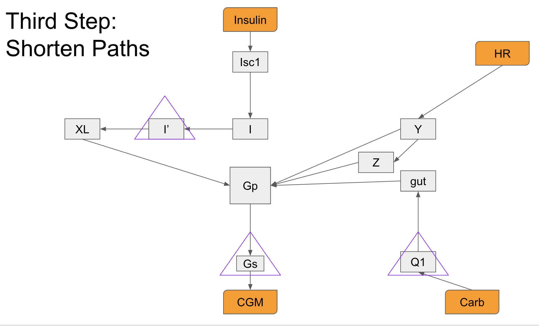
   (a) Paths to be Shortened in the Starting Graph

   

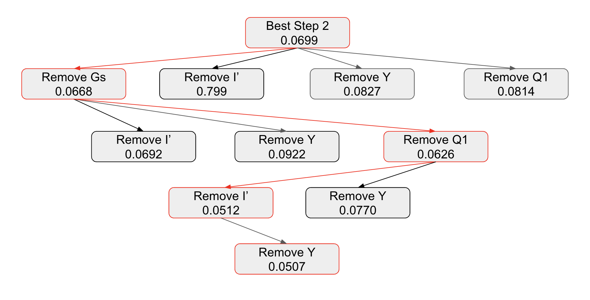
   (b) Reduction Tree of the Path Shortening Step

   

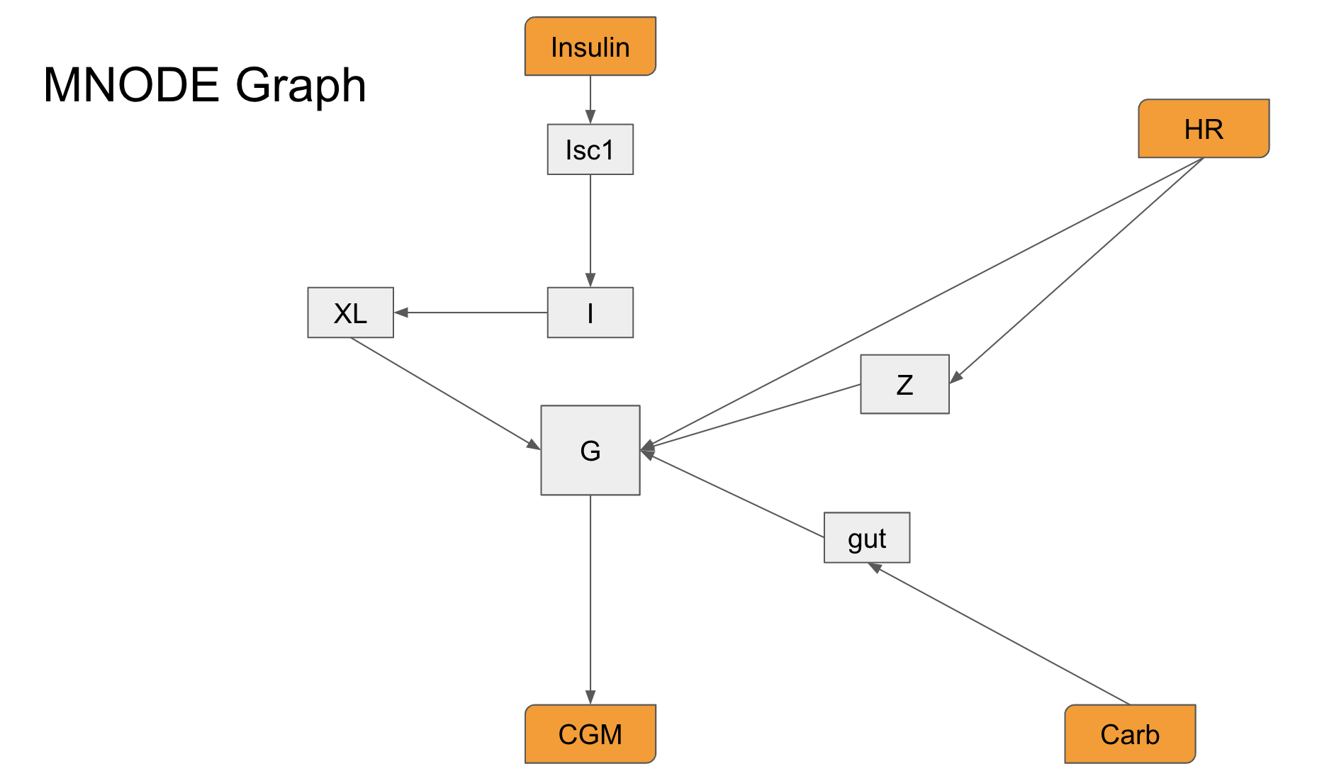
   (c) End Graph of the Path Shortening Step

   Figure 9: Illustration of the Combining Non-overlapping Paths Step of Our Heuristic

   The final graph we use for MNODE is therefore Figure 10, we showed it again with larger size for better readability.

   

   Figure 10: Final Graph used by MNODE

Appendix D Detailed Data Preparation Procedure

Here we provide a step-by-step procedure of how we pre-processed the T1DEXI

We select patients on open-loop pumps with age under 40 and body mass index (BMI) less than 30. And among the selected patient, we keep exercises that lasted for at least 30 minutes.

For each selected exercise instance, we focus on the time window from 4 hours before the beginning of exercise to 30 minutes after the beginning of exercise. As CGM readings are taken every 5 minutes for all patients in T1DEXI, this 270-minute window should correspond to 54 entries (5 minutes apart) in CGM data. These 54 entries will form the first feature of the time series representation of this exercise and the time stamps of these 54 entries will be the time stamps of the time series. Next we move to extract insulin and meal data. For each time stamp of the time series, we scan the insulin injection/carbohydrate consumption data files and if the patient had injected insulin/consumed carbohydrate between this time stamp and the next, we add the recorded amount to the 2nd/3rd feature of the time series at this time stamp. Note that for insulin we consider both basal insulin and bolus insulin injections. Next, we scan the heart rate/step count file, and set the 4th/5th feature of time series to be the average heart rate/step count recorded between the corresponding time stamp and the next. After this step, one should end up with a time series of 54 time steps and 5 features for each selected exercise instance.

The next major step is to prepare the intervention sets. For each exercise time series, we first create an intervention set containing three copies of the original time series. And then we uniformly randomly (simulated by a numpy default random number generator with seed 2024) apply one of the four following intervention sets to it:

1. Add 0/50/100 grams of carbohydrate to the three copies at the beginning of exercise (the 7th last time step),

2. Add 0/2.5/5 units of insulin to the three copies throughout exercise (the last 7 time steps),

3. Add nothing/50 grams of carb/10 units of insulin to the three copies at the beginning of exercise,

4. Change the recorded heart rate in the last 7 time steps to typical medium intensity aerobic (80,90,100,110,120,130,120)/ typical interval (80,170,80,170,80,170,80)/typical high intensity resistance (160,170,180,170,160,180,160).

To make sure the labels are not always the same for the same type of intervention, we then switch the 2nd and the 3rd copy with probability 0.5 (again simulated with the same numpy random number generator). Finally we compute the corresponding class label of the intervention set and add it to the causal task solution data set. At the end of this step, for each exercise instance, one should end up with a 4-stack time series of shape (4,54,5).

Next, we perform a round of data cleaning. We removed exercise instances with 0 or nan in heart rate feature, and replaced nan in other features with 0. After this step, we ended up with 94 exercise instances, forming a data set of size (94,4,54,5) and a causal task solution set of size (94,3).

Appendix E Model Implementations and Hyperparameters

Set-up

For each model mentioned in the experiment section, here we offer a detailed description of its computation equations and the hyperparameters used. Throughout this section we are given an exercise time series of 54 time steps (corresponding to 54 5-min intervals that made up the time window starting from 4 hours before exercise and ending at 30 minutes after the onset of exercise) and 5 features (corresponding to CGM reading, insulin, carbohydrate, heart rate and step count in order). We will denote the first feature (CGM reading) as $y$ and the rest 4 features as $x$. We will use subscript to indicate discrete time steps and superscript to indicate feature indices. For example, $x_{1}^{2}$ is the 2nd feature of $x$ (carbohydrate) at discrete time step $t=1$. To better indicate past and future, we set the 7th last entry to be $t=0$ and define 1 step of time to be 5 minutes. Our goal is to predict the CGM trace during the first 30 minutes of exercise corresponding to the expected output $y_{1:6}\in\mathbb{R}^{6}$ and therefore we set the number of prediction steps $q$ to be 6 for all models. We further split the given time series into historical context $p=(y,x)_{-47:-1}\in\mathbb{R}^{47\times 5}$, starting glucose $y_{0}\in\mathbb{R}$, inputs during exercise $x_{0:5}\in\mathbb{R}^{6\times 4}$ (six inputs that are recorded 1 time step ahead of the expected outputs). We use $\hat{y}\in\mathbb{R}^{6}$ to indicate the CGM trace predicted by models, $s$ for modeled states and $z$ for latent states. $h,c$ for the final hidden state and cell state of the LSTM initial condition learner. For ease of computation and without loss of generality, we set the $\Delta t$ term in forward-Euler style discretization to be $1$ for all relevant models, and thus we omit it in the equations.

Learning Rate, Training Epochs and Optimizer

Also for all models, we set the default learning rate to be $2\cdot 10^{-3}$ and use the Adam optimizer (Kingma and Ba, 2014). Unless otherwise specified in the model description, we train for 100 epochs and pick the best epoch with a validation set. For each model we tested this learning rate and training epoch on an initial try-it-out run and found them to be robust for all the models (in most cases training error converges within first 50 epochs). While we understand that the best practice is to always tune learning rates, here we made the decision not to tune it in an attempt to reduce the dimension of the hyperparameter search space, which is already very large for some models. Since Adam already adjusts learning rate for each parameter in the model, we did not see significant variation in model performance with other learning rates.

Dropout

One may notice that for the hybrid models, we place 0 dropout rate on the MLPs. This is because we are already doing regularization via epoch selection based on validation set, and our trial runs indicate that there is no need for additional regularization (adding any non-zero dropout for hybrid models worsens performance). This is not true for black-box models, for which we still tune the dropout rate.

Hyperparameter Search

We use grid search to tune hyperparameters. When choosing the grid, we restrict the search space to areas where the models have less than 25000 parameters and we also try to limit the number of grid points to around 10. This is to make sure the computational cost of the experiments is capped at a reasonable level for small data sets and individual users.

E.1 UVA

UVA is our baseline mechanisitc model, whose description is given in Appendix A. The computation equation for the UVA model is given in Algorithm 1.

Algorithm 1 UVA Padova Model

  Input: number of prediction steps $q=6$, historical context $p$, starting glucose $y_{0}$, exogenous inputs $x_{0:5}$, the original UVA mechanistic ODEs $m_{\text{UVA}}$, $\Delta t=1$

  $h,c=\text{LSTM}(p)$

  $h^{1}=y_{0}$

  $s_{0}=h$

  for $i=0:q-1$ do

     $s_{i+1}=s_{i}+\Delta t\cdot m_{\text{UVA}}(s_{i},x_{i};\beta)$

     $\hat{y}_{i+1}=s_{t+1}^{1}$

  end for

  Output: $\hat{y}_{1:q}$

Inside the algorithm, the LSTM network has 2 layers and 21 hidden dimensions (same as the UVA/Padova model), and we set the first state of the estimated initial condition (represented by hidden state $h$) to be the true initial value of CGM $y_{0}$ to keep consistency with the assumption that $s^{1}$ represents glucose. The UVA/Padova Simulator has 52 trainable parameters $\beta\in\mathbb{R}^{52}$. We do not tune hyperparameters for the UVA model as there are not meaningful hyperparameters to tune.

E.2 Reduced UVA Latent Parameter Learning

The Reduced UVA Latent Parameter Learning model uses a lower-fidelity, reduced version of UVA/Padova defined in Appendix B, and applies the idea of latent parameter learning to it. The computation equations are given in Algorithm 2

Algorithm 2 Reduced UVA Latent Parameter Learning Model

  Input: number of prediction steps $q$, historical context $p$, starting glucose $y_{0}$, exogenous inputs $x$, the reduced UVA mechanistic ODEs $m_{\text{RUVA}}$, $\Delta t=1$

  $h,c=\text{LSTM}(p)$

  $s_{0}=\text{concatenate}(y0,\text{MLP1}(h))$

  $z_{0}=c$

  for $i=0:q-1$ do

     $s_{i+1}=s_{i}+\Delta t\cdot m_{\text{RUVA}}(s_{i},x_{i};\beta_{i}=\text{MLP2}(z_{i}))$

     $z_{i+1}=Az_{i}+Bx_{i}^{3\sim 4}$

     $\hat{y}_{i+1}=s_{t+1}^{1}$

  end for

  Output: $\hat{y}_{1:q}$

Note in the above implementation, the latent dynamics of $z$ only depends on itself and inputs that are not used by the UVA S2013 model (the 3rd and 4th feature, which correspond to heart rate and step count). We made this choice to keep consistency with the implementation in Miller et al. (2020). The LSTM has 2 layers and $d$ hidden dimension (since this time the cell states are used to initialize latent state $z$, whose dimension needs to be tuned) and MLP2 serves to map $d$ dimensional $h_{0}$ to a 8-dimensional initial condition vector. All MLPs have $n$ hidden layers and $m$ hidden units with dropout $0$ and activation ReLu, we tune these hyperpameters with grid search on the following grid:

$$n=\{2,3,4\}\times m=\{16,32,48\}\times d=\{8,12,16\}$$

E.3 Reduced UVA Latent Parameter and State Closure Learning

The Reduced UVA Latent Parameter and State Closure Learning model uses the same reduced UVA/Padova defined in Appendix B, and applies both the idea of latent parameter learning and state closure learning to it. The computation equations are given in Algorithm 3

Algorithm 3 Reduced UVA Latent Parameter and State Closure Learning Model

  Input: number of prediction steps $q=6$, historical context $p$, starting glucose $y_{0}$, exogenous inputs $x_{0:5}$, the reduced UVA mechanistic ODEs $m_{\text{RUVA}}$ the adjacency matrices (as defined in Section 3) of reduced UVA: $A_{s},A_{x}$, closure switch constant $c$, $\Delta t=1$

  $h,c=\text{LSTM}(p)$

  $s_{0}=\text{concatenate}(y_{0},\text{MLP1}(h))$

  $z_{0}=c$

  for $i=0:q-1$ do

     $s_{i+1}=s_{i}+\Delta t\cdot m_{\text{RUVA}}(s_{i},x_{i};\beta_{i}=\text{MLP2}(z_{i}))+c\cdot\text{MLPs}(s_{i},x_{i};A_{s},A_{x})$

     $z_{i+1}=Az_{i}+Bx_{i}^{3\sim 4}$

     $\hat{y}_{i+1}=s_{t+1}^{1}$

  end for

  Output: $\hat{y}_{1:q}$

The LSTM has 2 layers and $d$ hidden dimension (since this time the cell states are used to initialize latent state $z$, whose dimension needs to be tuned). MLP1 and MLP2 have $n$ hidden layers and $m$ hidden units with dropout $0$ and activation ReLu, while MLPs that form the closure learning network have $2$ hidden layers and $m$ hidden units with dropout $0$ and activation ReLu. We tune these hyperpameters with grid search on the following grid:

$$n=\{2,3\}\times m=\{16,24,32\}\times d=\{8,16\}$$

Note that our search space is smaller as the introduction of extra MLPs significantly increases the total number of parameters.

The training routine of models adopting state closure is more complicated. We first set $c=0$ and just train the reduced UVA latent parameter model and the initial condition learner LSTM for 100 epochs (the closure part is masked out by $c$). Then we freeze the weights of the reduced UVA latent parameter model and the LSTM, set $c=1$ and train the closure neural network on the residuals for 50 more epochs. This trick makes sure the closure network is truly learning the residuals as intended and not subsuming the mechanistic model.

E.4 Mechanistic Neural ODE

The MNODE model no longer relies on the functional forms of UVA models, and therefore does not require any ODE equations $m$. Instead, it uses the adjacency matrices of a reduced version of the UVA/Padova graph. We obtain this reduced graph with the reduction heuristic described in Appendix C. We provide its computation equations in Algorithm 4.

Algorithm 4 Mechanistic Neural ODE Model

  Input: number of prediction steps $q=6$, historical context $p$,starting glucose $y_{0}$, exogenous inputs $x_{0:5}$, the adjacency matrices (as defined in Section 3) of the reduced UVA graph $A_{s},A_{x}$, $\Delta t=1$

  $h,c=\text{LSTM}(p)$

  $h^{1}=y_{0}$

  $s_{0}=h$

  for $i=0:q-1$ do

     $s_{i+1}=s_{i}+\Delta t\cdot\text{MLPs}(s_{i},x_{i};A_{s},A_{x})$

     $\hat{y}_{i+1}=s_{t+1}^{1}$

  end for

  Output: $\hat{y}_{1:q}$

The LSTM has 2 layers and $5$ hidden dimension (this corresponds to the number of states in the reduced graph) and for the same reason we set the 1st features of the initial condition state vector to be $y_{0}$. All MLPs have $n$ hidden layers and $m$ hidden units with dropout $0$ and activation ReLu, we tune these hyperpameters with grid search on the following grid:

$$n=\{2,3\}\times m=\{16,24,32\}.$$

E.5 BNODE

For BNODE and the subsequent black-box models, we do not provide design rationales behind them as it is better to refer to their original author for such details. Instead, we simply describe our how we implemented them.

Algorithm 5 Black-box Neural ODE Model

  Input: number of prediction steps $q=6$, historical context $p$, starting glucose $y_{0}$, exogenous inputs $x_{0:5}$, $\Delta t=1$

  $h,c=\text{LSTM}(p)$

  $h^{1}=y_{0}$

  $s_{0}=h$

  for $i=0:q-1$ do

     $s_{i+1}=s_{i}+\Delta t\cdot\text{MLPs}(s_{i},x_{i})$

     $\hat{y}_{i+1}=s_{t+1}^{1}$

  end for

  Output: $\hat{y}_{1:q}$

The LSTM has 2 layers and $d$ hidden dimension. Note that here the hidden dimension of LSTM also determines the state dimension of the neural ODE, which is a tunable hyperparameter. All MLPs have $n$ hidden layers and $m$ hidden units with dropout $a$ and activation ReLu, we tune these hyperpameters with grid search on the following grid:

$$d=\{4,5,6\}\times n=\{2,3\}\times m=\{32,48,60\}\times a=\{0,0.1,0.2\}.$$

E.6 TCN

Algorithm 6 Temporal Convolutional Network Model

  Input: number of prediction steps $q=6$, historical context $p$, starting glucose $y_{0}$, exogenous inputs $x_{0:5}$

  $\tilde{x}=\mathbf{0}\in\mathbb{R}^{q}$

  $\tilde{x}_{0}=y_{0}$

  $x^{\prime}=\text{concatenate}(\tilde{x},x,\text{dim}=-1)$

  $seq_{in}=\text{concatenate}(p,x^{\prime},\text{dim}=0)$

  $seq_{out}=\text{TCN}(seq_{i}n)$

  $\hat{y}=\text{Linear}(seq_{out})$

  Output: $\hat{y}$

The TCN model is taken directly from the code repository posted on https://github.com/locuslab/TCN/blob/master/TCN/tcn.py, with input size set to 5, output size set to 6, number of channels set to a list of $n$ copies of $m$, kernel size set to $l$ and dropout set to $a$. We tune these hyperpameters with grid search on the following grid:

$$n=\{2,3\}\times m=\{16,24,32\}\times l=\{2,3,4\}\times a=\{0,0.1,0.2\}.$$

E.7 LSTM

Algorithm 7 Long Short Term Memory Model

  Input: number of prediction steps $q=6$, historical context $p$, starting glucose $y_{0}$, exogenous inputs $x_{0:5}$

  $h,c=\text{Encoder LSTM}(p)$

  Set initial hidden state and cell state of Decoder LSTM to $h,c$ respectively

  $seq_{out}h_{q},c_{q}=\text{Decoder LSTM}(x_{0:5})$

  $\hat{y}=\text{Linear}(seq_{out})$

  Output: $\hat{y}$

Both Encoder and Decoder LSTM have $n$ layers and $d$ hidden states with dropout set to $a$. We tune these hyperpameters with grid search on the following grid:

$$n=\{2,3.4\}\times m=\{8,12,16\}\times a=\{0,0.1,0.2\}.$$

E.8 Transformer

Algorithm 8 Transformer Model

  Input: number of prediction steps $q=6$, historical context $p$, starting glucose $y_{0}$, exogenous inputs $x_{0:5}$, true output $y_{1:5}$ (needed during training)

  $\tilde{x}=\mathbf{0}\in\mathbb{R}^{q}$

  $\tilde{x}_{0}=y_{0}$

  $x^{\prime}=\text{concatenate}(\tilde{x},x,\text{dim}=-1)$

  $\text{encoder\_in}=\text{concatenate}(p,x^{\prime},\text{dim}=0)$ (concatenating all inputs to form a masked context)

  if Model in Training Mode then

     $\text{decoder\_in}=\text{concatenate}(y_{0},y_{1:5})$ (expected output shifted to the right)

     $\text{decode\_out}=\text{Transformer}(\text{encoder\_in},\text{decoder\_in},\text{decoder\_causal\_mask})$

  end if

  if Model in Evaluation Mode then

     $\text{decoder\_in}=\text{concatenate}(y_{0},\mathbf{0}\in\mathbb{R}^{q-1})$

     for $i=1:q-1$ do

        $\text{decode\_out}=\text{Transformer}(\text{encoder\_in},\text{decoder\_in},\text{decoder\_causal\_mask})$

        $\text{decoder\_in}_{i+1}=\text{decode\_out}_{i}$

     end for

     $\text{decode\_out}=\text{Transformer}(\text{encoder\_in},\text{decoder\_in},\text{decoder\_causal\_mask})$

  end if

  $y=\text{Linear}(\text{decode\_out})$

  Output: $y$

We use the transformer model provided by the pytorch nn class, and its hyperparameters are set as follows: d_model set to $n$, number of encoder layers and number of decoder layers are both set to 3, the dim_feedforward is set to $m$ and dropout is set to $a$. We tune the hyperparameters with the following grid:

$$n=\{8,16\}\times m=\{32,64\}\times a=\{0,0.1,0.2\}$$

E.9 S4D

Algorithm 9 S4 Diagonal Model

  Input: number of prediction steps $q=6$, historical context $p$, starting glucose $y_{0}$, exogenous inputs $x_{0:5}$

  $\tilde{x}=\mathbf{0}\in\mathbb{R}^{q}$

  $\tilde{x}_{0}=y_{0}$

  $x^{\prime}=\text{concatenate}(\tilde{x},x_{0:5},\text{dim}=-1)$

  $seq_{in}=\text{concatenate}(p,x^{\prime},\text{dim}=0)$

  $seq_{out}=\text{S4D}(seq_{i}n)$

  $\hat{y}=\text{Linear}(seq_{out})_{-6:}$

  Output: $\hat{y}$

We take the S4D model directly from the following github repository https://github.com/thjashin/multires-conv/blob/main/layers/s4d.py, and its hyperparameters are set as: d_model set to $53$, d_state set to $m$, dropout set to $a$.We tune the hyperparameters with the following grid:

$$m=\{32,64,128\}\times a=\{0,0.1,0.2\}$$

Appendix F Repeated Nested Cross Validation

We use the following algorithm to evaluate both predictive and causal generalization errors of our models.

Algorithm 10 Repeated Nested Cross Validation

  Input: Data $D$, Model $M$, Hybrid Loss Function $l_{h}$, Alpha for Hybrid Loss $\alpha$, List of Hyperparameter Settings $\Lambda$,Number of Repeats $R=3$, Number of Outer Fold $N=6$, Number of Inner Fold $M=4$, Random Seed $s=2024$

  Generate $R$ different permutations of $[1,\dots,\text{length}(D)]$: $P_{1},\dots,P_{R}$ with numpy default random number generator and seed $s$

  Initialize Error Lists $e_{\text{pred}},e_{\text{causal}}$

  for $r=1:R$ do

     Permute $D$ with permutation $P_{r}$, save the resulting data as $D_{r}$

     Split $D_{r}$ into $N$ folds $D_{r}^{1},\dots D_{r}^{N}$

     for $i=1:N$ do

        Form the outer training set as $D_{\text{tout}}=D_{r}\setminus D_{r}^{i}$, and set the test set as $D_{\text{test}}=D_{r}^{i}$

        Split $D_{\text{tout}}$ into M folds $D_{\text{tout}}^{1},\dots,D_{\text{tout}}^{M}$

        for $j=1:M$ do

           Form the training set as $D_{\text{train}}=D_{\text{tout}}\setminus D_{\text{tout}}^{j}$

           Form the validation set as $D_{\text{val}}=D_{\text{tout}}^{j}$

           if $j<M$ then

              for each $\lambda\in\Lambda$ do

                 Set pytorch seed to $s-1=2023$

                 Standardize $D_{\text{train}},D_{\text{val}},D_{\text{test}}$ with sample mean and standard deviation of $D_{\text{train}}$

                 Train $M$ on $D_{\text{train}}$ with hyperparameter setting $\lambda$, add the best validation hybrid loss $l_{h}(\cdot,D_{\text{val}};\alpha)$ achieved during training to the score of $\lambda$

              end for

           end if

           if $j=M$ then

              Select $\lambda^{*}$ from $\Lambda$ with the lowest score

              Set pytorch seed to $s-1=2023$

              Standardize $D_{\text{train}},D_{\text{val}},D_{\text{test}}$ with sample mean and standard deviation of $D_{\text{train}}$

              Train $M$ on $D_{\text{train}}$ with hyperparameter setting $\lambda^{*}$, select the epoch $M^{*}$ with best validation hybrid loss $l_{h}(\cdot,D_{\text{val}};\alpha)$.

              Add $l_{h}(M^{*},D_{\text{test}};\alpha=0)$ to $e_{\text{pred}}$

              Add $l_{h}(M^{*},D_{\text{test}};\alpha=1)$ to $e_{\text{causal}}$

           end if

        end for

     end for

  end for

  Output: $e_{\text{pred}},e_{\text{causal}}$

References

- Allen et al. (2023) Kelsey R Allen, Tatiana Lopez Guevara, Yulia Rubanova, Kim Stachenfeld, Alvaro Sanchez-Gonzalez, Peter Battaglia, and Tobias Pfaff. Graph network simulators can learn discontinuous, rigid contact dynamics. In Conference on Robot Learning, pages 1157–1167. PMLR, 2023.
- Asikis et al. (2022) Thomas Asikis, Lucas Böttcher, and Nino Antulov-Fantulin. Neural ordinary differential equation control of dynamics on graphs. Physical Review Research, 4(1):013221, 2022.
- Ayed et al. (2019) Ibrahim Ayed, Emmanuel de Bézenac, Arthur Pajot, Julien Brajard, and Patrick Gallinari. Learning dynamical systems from partial observations. arXiv preprint arXiv:1902.11136, 2019.
- Bai et al. (2018) Shaojie Bai, J Zico Kolter, and Vladlen Koltun. An empirical evaluation of generic convolutional and recurrent networks for sequence modeling. arXiv preprint arXiv:1803.01271, 2018.
- Bisgaard Bengtsen and Møller (2021) Mads Bisgaard Bengtsen and Niels Møller. Mini-review: Glucagon responses in type 1 diabetes–a matter of complexity. Physiological Reports, 9(16):e15009, 2021.
- Bishnoi et al. (2022) Suresh Bishnoi, Ravinder Bhattoo, Sayan Ranu, and NM Krishnan. Enhancing the inductive biases of graph neural ode for modeling dynamical systems. arXiv preprint arXiv:2209.10740, 2022.
- Brajard et al. (2021) Julien Brajard, Alberto Carrassi, Marc Bocquet, and Laurent Bertino. Combining data assimilation and machine learning to infer unresolved scale parametrization. Philosophical Transactions of the Royal Society A, 379(2194):20200086, 2021.
- Brazeau et al. (2008) Anne-Sophie Brazeau, Rémi Rabasa-Lhoret, Irene Strychar, and Hortensia Mircescu. Barriers to physical activity among patients with type 1 diabetes. Diabetes care, 31(11):2108–2109, 2008.
- Canini and Perelson (2014) Laetitia Canini and Alan S Perelson. Viral kinetic modeling: state of the art. Journal of pharmacokinetics and pharmacodynamics, 41:431–443, 2014.
- Chen et al. (2018) Ricky TQ Chen, Yulia Rubanova, Jesse Bettencourt, and David K Duvenaud. Neural ordinary differential equations. Advances in neural information processing systems, 31, 2018.
- Chen et al. (2022) Yuming Chen, Daniel Sanz-Alonso, and Rebecca Willett. Autodifferentiable ensemble kalman filters. SIAM Journal on Mathematics of Data Science, 4(2):801–833, 2022.
- Chung et al. (2014) Junyoung Chung, Caglar Gulcehre, KyungHyun Cho, and Yoshua Bengio. Empirical evaluation of gated recurrent neural networks on sequence modeling. arXiv preprint arXiv:1412.3555, 2014.
- Dalla Man et al. (2009) Chiara Dalla Man, Marc D Breton, and Claudio Cobelli. Physical activity into the meal glucose—insulin model of type 1 diabetes: In silico studies, 2009.
- Deichmann et al. (2023) Julia Deichmann, Sara Bachmann, Marie-Anne Burckhardt, Marc Pfister, Gabor Szinnai, and Hans-Michael Kaltenbach. New model of glucose-insulin regulation characterizes effects of physical activity and facilitates personalized treatment evaluation in children and adults with type 1 diabetes. PLOS Computational Biology, 19(2):e1010289, 2023.
- Didona et al. (2015) Diego Didona, Francesco Quaglia, Paolo Romano, and Ennio Torre. Enhancing performance prediction robustness by combining analytical modeling and machine learning. In Proceedings of the 6th ACM/SPEC international conference on performance engineering, pages 145–156, 2015.
- Du et al. (2019) Mengnan Du, Ninghao Liu, and Xia Hu. Techniques for interpretable machine learning. Communications of the ACM, 63(1):68–77, 2019.
- Gu et al. (2021) Albert Gu, Karan Goel, and Christopher Ré. Efficiently modeling long sequences with structured state spaces. arXiv preprint arXiv:2111.00396, 2021.
- Gu et al. (2022) Albert Gu, Karan Goel, Ankit Gupta, and Christopher Ré. On the parameterization and initialization of diagonal state space models. Advances in Neural Information Processing Systems, 35:35971–35983, 2022.
- Gupta and Lermusiaux (2021) Abhinav Gupta and Pierre FJ Lermusiaux. Neural closure models for dynamical systems. Proceedings of the Royal Society A, 477(2252):20201004, 2021.
- Haber and Ruthotto (2017) Eldad Haber and Lars Ruthotto. Stable architectures for deep neural networks. Inverse problems, 34(1):014004, 2017.
- He et al. (2016) Kaiming He, Xiangyu Zhang, Shaoqing Ren, and Jian Sun. Deep residual learning for image recognition. In Proceedings of the IEEE conference on computer vision and pattern recognition, pages 770–778, 2016.
- He et al. (2020) Shaobo He, Yuexi Peng, and Kehui Sun. Seir modeling of the covid-19 and its dynamics. Nonlinear dynamics, 101:1667–1680, 2020.
- Hilgemann and Noble (1987) DW Hilgemann and Denis Noble. Excitation-contraction coupling and extracellular calcium transients in rabbit atrium: reconstruction of basic cellular mechanisms. Proceedings of the Royal society of London. Series B. Biological sciences, 230(1259):163–205, 1987.
- Hobbs et al. (2019) Nicole Hobbs, Iman Hajizadeh, Mudassir Rashid, Kamuran Turksoy, Marc Breton, and Ali Cinar. Improving glucose prediction accuracy in physically active adolescents with type 1 diabetes. Journal of diabetes science and technology, 13(4):718–727, 2019.
- Hochreiter and Schmidhuber (1997) Sepp Hochreiter and Jürgen Schmidhuber. Long short-term memory. Neural computation, 9(8):1735–1780, 1997.
- Hodgkin and Huxley (1952) Alan L Hodgkin and Andrew F Huxley. A quantitative description of membrane current and its application to conduction and excitation in nerve. The Journal of physiology, 117(4):500, 1952.
- Holz and Fahr (2001) Martin Holz and Alfred Fahr. Compartment modeling. Advanced Drug Delivery Reviews, 48(2-3):249–264, 2001.
- Hussain et al. (2021) Zeshan M Hussain, Rahul G Krishnan, and David Sontag. Neural pharmacodynamic state space modeling. In International Conference on Machine Learning, pages 4500–4510. PMLR, 2021.
- Jin et al. (2022) Ming Jin, Yu Zheng, Yuan-Fang Li, Siheng Chen, Bin Yang, and Shirui Pan. Multivariate time series forecasting with dynamic graph neural odes. IEEE Transactions on Knowledge and Data Engineering, 2022.
- Karniadakis et al. (2021) George Em Karniadakis, Ioannis G Kevrekidis, Lu Lu, Paris Perdikaris, Sifan Wang, and Liu Yang. Physics-informed machine learning. Nature Reviews Physics, 3(6):422–440, 2021.
- Kidger (2022) Patrick Kidger. On neural differential equations, 2022.
- Kingma and Ba (2014) Diederik P Kingma and Jimmy Ba. Adam: A method for stochastic optimization. arXiv preprint arXiv:1412.6980, 2014.
- Ladenbauer et al. (2019) Josef Ladenbauer, Sam McKenzie, Daniel Fine English, Olivier Hagens, and Srdjan Ostojic. Inferring and validating mechanistic models of neural microcircuits based on spike-train data. Nature communications, 10(1):4933, 2019.
- Lea et al. (2016) Colin Lea, Rene Vidal, Austin Reiter, and Gregory D Hager. Temporal convolutional networks: A unified approach to action segmentation. In Computer Vision–ECCV 2016 Workshops: Amsterdam, The Netherlands, October 8-10 and 15-16, 2016, Proceedings, Part III 14, pages 47–54. Springer, 2016.
- Levine and Stuart (2022) Matthew Levine and Andrew Stuart. A framework for machine learning of model error in dynamical systems. Communications of the American Mathematical Society, 2(07):283–344, 2022.
- Li et al. (2022) Zijie Li, Kazem Meidani, Prakarsh Yadav, and Amir Barati Farimani. Graph neural networks accelerated molecular dynamics. The Journal of Chemical Physics, 156(14), 2022.
- Liu et al. (2018) Chengyuan Liu, Josep Vehi, Nick Oliver, Pantelis Georgiou, and Pau Herrero. Enhancing blood glucose prediction with meal absorption and physical exercise information. arXiv preprint arXiv:1901.07467, 2018.
- Lu et al. (2021) James Lu, Kaiwen Deng, Xinyuan Zhang, Gengbo Liu, and Yuanfang Guan. Neural-ode for pharmacokinetics modeling and its advantage to alternative machine learning models in predicting new dosing regimens. Iscience, 24(7), 2021.
- Man et al. (2014) Chiara Dalla Man, Francesco Micheletto, Dayu Lv, Marc Breton, Boris Kovatchev, and Claudio Cobelli. The uva/padova type 1 diabetes simulator: new features. Journal of diabetes science and technology, 8(1):26–34, 2014.
- Marsh et al. (2005) Donald J Marsh, Olga V Sosnovtseva, Ki H Chon, and Niels-Henrik Holstein-Rathlou. Nonlinear interactions in renal blood flow regulation. American Journal of Physiology-Regulatory, Integrative and Comparative Physiology, 288(5):R1143–R1159, 2005.
- McArdle et al. (2006) William D McArdle, Frank I Katch, and Victor L Katch. Essentials of exercise physiology. Lippincott Williams & Wilkins, 2006.
- Miller et al. (2020) Andrew C Miller, Nicholas J Foti, and Emily Fox. Learning insulin-glucose dynamics in the wild. In Machine Learning for Healthcare Conference, pages 172–197. PMLR, 2020.
- Oviedo et al. (2017) Silvia Oviedo, Josep Vehí, Remei Calm, and Joaquim Armengol. A review of personalized blood glucose prediction strategies for t1dm patients. International journal for numerical methods in biomedical engineering, 33(6):e2833, 2017.
- Owoyele and Pal (2022) Opeoluwa Owoyele and Pinaki Pal. Chemnode: A neural ordinary differential equations framework for efficient chemical kinetic solvers. Energy and AI, 7:100118, 2022.
- Passini et al. (2017) Elisa Passini, Oliver J Britton, Hua Rong Lu, Jutta Rohrbacher, An N Hermans, David J Gallacher, Robert JH Greig, Alfonso Bueno-Orovio, and Blanca Rodriguez. Human in silico drug trials demonstrate higher accuracy than animal models in predicting clinical pro-arrhythmic cardiotoxicity. Frontiers in physiology, 8:668, 2017.
- Pathak et al. (2018) Jaideep Pathak, Alexander Wikner, Rebeckah Fussell, Sarthak Chandra, Brian R Hunt, Michelle Girvan, and Edward Ott. Hybrid forecasting of chaotic processes: Using machine learning in conjunction with a knowledge-based model. Chaos: An Interdisciplinary Journal of Nonlinear Science, 28(4):041101, 2018.
- Pearl (1998) Judea Pearl. Graphs, causality, and structural equation models. Sociological Methods & Research, 27(2):226–284, 1998.
- Perelson et al. (1996) Alan S Perelson, Avidan U Neumann, Martin Markowitz, John M Leonard, and David D Ho. Hiv-1 dynamics in vivo: virion clearance rate, infected cell life-span, and viral generation time. Science, 271(5255):1582–1586, 1996.
- Pfaff et al. (2020) Tobias Pfaff, Meire Fortunato, Alvaro Sanchez-Gonzalez, and Peter W Battaglia. Learning mesh-based simulation with graph networks. arXiv preprint arXiv:2010.03409, 2020.
- Poli et al. (2019) Michael Poli, Stefano Massaroli, Junyoung Park, Atsushi Yamashita, Hajime Asama, and Jinkyoo Park. Graph neural ordinary differential equations. arXiv preprint arXiv:1911.07532, 2019.
- Qian et al. (2021) Zhaozhi Qian, William Zame, Lucas Fleuren, Paul Elbers, and Mihaela van der Schaar. Integrating expert odes into neural odes: pharmacology and disease progression. Advances in Neural Information Processing Systems, 34:11364–11383, 2021.
- Rackauckas et al. (2020) Christopher Rackauckas, Yingbo Ma, Julius Martensen, Collin Warner, Kirill Zubov, Rohit Supekar, Dominic Skinner, Ali Ramadhan, and Alan Edelman. Universal differential equations for scientific machine learning. arXiv preprint arXiv:2001.04385, 2020.
- Raissi et al. (2019) Maziar Raissi, Paris Perdikaris, and George E Karniadakis. Physics-informed neural networks: A deep learning framework for solving forward and inverse problems involving nonlinear partial differential equations. Journal of Computational physics, 378:686–707, 2019.
- Ribera et al. (2022) H. Ribera, S. Shirman, A. V. Nguyen, and N. M. Mangan. Model selection of chaotic systems from data with hidden variables using sparse data assimilation. Chaos: An Interdisciplinary Journal of Nonlinear Science, 32(6), June 2022. ISSN 1089-7682. doi: 10.1063/5.0066066. URL http://dx.doi.org/10.1063/5.0066066.
- Rico-Martinez et al. (1994) R Rico-Martinez, JS Anderson, and IG Kevrekidis. Continuous-time nonlinear signal processing: a neural network based approach for gray box identification. In Proceedings of IEEE Workshop on Neural Networks for Signal Processing, pages 596–605. IEEE, 1994.
- Rico-Martinez et al. (1992) Ramiro Rico-Martinez, K Krischer, IG Kevrekidis, MC Kube, and JL Hudson. Discrete-vs. continuous-time nonlinear signal processing of cu electrodissolution data. Chemical Engineering Communications, 118(1):25–48, 1992.
- Riddell et al. (2017) Michael C Riddell, Ian W Gallen, Carmel E Smart, Craig E Taplin, Peter Adolfsson, Alistair N Lumb, Aaron Kowalski, Remi Rabasa-Lhoret, Rory J McCrimmon, Carin Hume, et al. Exercise management in type 1 diabetes: a consensus statement. The lancet Diabetes & endocrinology, 5(5):377–390, 2017.
- Riddell et al. (2023) Michael C Riddell, Zoey Li, Robin L Gal, Peter Calhoun, Peter G Jacobs, Mark A Clements, Corby K Martin, Francis J Doyle III, Susana R Patton, Jessica R Castle, et al. Examining the acute glycemic effects of different types of structured exercise sessions in type 1 diabetes in a real-world setting: The type 1 diabetes and exercise initiative (t1dexi). Diabetes care, 46(4):704–713, 2023.
- Sanchez-Gonzalez et al. (2018) Alvaro Sanchez-Gonzalez, Nicolas Heess, Jost Tobias Springenberg, Josh Merel, Martin Riedmiller, Raia Hadsell, and Peter Battaglia. Graph networks as learnable physics engines for inference and control. In International Conference on Machine Learning, pages 4470–4479. PMLR, 2018.
- Sanchez-Gonzalez et al. (2020) Alvaro Sanchez-Gonzalez, Jonathan Godwin, Tobias Pfaff, Rex Ying, Jure Leskovec, and Peter Battaglia. Learning to simulate complex physics with graph networks. In International conference on machine learning, pages 8459–8468. PMLR, 2020.
- Shi et al. (2023) Jiaxin Shi, Ke Alexander Wang, and Emily Fox. Sequence modeling with multiresolution convolutional memory. In International Conference on Machine Learning, pages 31312–31327. PMLR, 2023.
- Sottile et al. (2021) Peter D Sottile, David Albers, Peter E DeWitt, Seth Russell, JN Stroh, David P Kao, Bonnie Adrian, Matthew E Levine, Ryan Mooney, Lenny Larchick, et al. Real-time electronic health record mortality prediction during the covid-19 pandemic: a prospective cohort study. Journal of the American Medical Informatics Association, 28(11):2354–2365, 2021.
- Tauschmann et al. (2022) Martin Tauschmann, Gregory Forlenza, Korey Hood, Roque Cardona-Hernandez, Elisa Giani, Christel Hendrieckx, Daniel J DeSalvo, Lori M Laffel, Banshi Saboo, Benjamin J Wheeler, et al. Ispad clinical practice consensus guidelines 2022: diabetes technologies: glucose monitoring. Pediatric Diabetes, 23(8):1390–1405, 2022.
- ten Tusscher et al. (2004) Kirsten HWJ ten Tusscher, Denis Noble, Peter-John Noble, and Alexander V Panfilov. A model for human ventricular tissue. American Journal of Physiology-Heart and Circulatory Physiology, 286(4):H1573–H1589, 2004.
- Tyler et al. (2022) Nichole S Tyler, Clara Mosquera-Lopez, Gavin M Young, Joseph El Youssef, Jessica R Castle, and Peter G Jacobs. Quantifying the impact of physical activity on future glucose trends using machine learning. Iscience, 25(3):103888, 2022.
- Wang et al. (2022) Lijing Wang, Aniruddha Adiga, Jiangzhuo Chen, Adam Sadilek, Srinivasan Venkatramanan, and Madhav Marathe. Causalgnn: Causal-based graph neural networks for spatio-temporal epidemic forecasting. In Proceedings of the AAAI conference on artificial intelligence, volume 36, pages 12191–12199, 2022.
- Weinan (2017) Ee Weinan. A proposal on machine learning via dynamical systems. Communications in Mathematics and Statistics, 1(5):1–11, 2017.
- Wellen et al. (2005) Kathryn E Wellen, Gökhan S Hotamisligil, et al. Inflammation, stress, and diabetes. The Journal of clinical investigation, 115(5):1111–1119, 2005.
- Willard et al. (2022) Jared Willard, Xiaowei Jia, Shaoming Xu, Michael Steinbach, and Vipin Kumar. Integrating scientific knowledge with machine learning for engineering and environmental systems. ACM Computing Surveys, 55(4):1–37, 2022.
- Wu et al. (2021) Haixu Wu, Jiehui Xu, Jianmin Wang, and Mingsheng Long. Autoformer: Decomposition transformers with auto-correlation for long-term series forecasting. Advances in Neural Information Processing Systems, 34:22419–22430, 2021.
- Wu et al. (2022) Tailin Wu, Qinchen Wang, Yinan Zhang, Rex Ying, Kaidi Cao, Rok Sosic, Ridwan Jalali, Hassan Hamam, Marko Maucec, and Jure Leskovec. Learning large-scale subsurface simulations with a hybrid graph network simulator. In Proceedings of the 28th ACM SIGKDD Conference on Knowledge Discovery and Data Mining, pages 4184–4194, 2022.
- Xia et al. (2021) Kevin Xia, Kai-Zhan Lee, Yoshua Bengio, and Elias Bareinboim. The causal-neural connection: Expressiveness, learnability, and inference. Advances in Neural Information Processing Systems, 34:10823–10836, 2021.
- Xia et al. (2022) Kevin Xia, Yushu Pan, and Elias Bareinboim. Neural causal models for counterfactual identification and estimation. arXiv preprint arXiv:2210.00035, 2022.
- Xie and Wang (2020) Jinyu Xie and Qian Wang. Benchmarking machine learning algorithms on blood glucose prediction for type i diabetes in comparison with classical time-series models. IEEE Transactions on Biomedical Engineering, 67(11):3101–3124, 2020.
- Yazdani et al. (2020) Alireza Yazdani, Lu Lu, Maziar Raissi, and George Em Karniadakis. Systems biology informed deep learning for inferring parameters and hidden dynamics. PLoS computational biology, 16(11):e1007575, 2020.
- Zhou et al. (2021) Haoyi Zhou, Shanghang Zhang, Jieqi Peng, Shuai Zhang, Jianxin Li, Hui Xiong, and Wancai Zhang. Informer: Beyond efficient transformer for long sequence time-series forecasting. In Proceedings of the AAAI conference on artificial intelligence, volume 35, pages 11106–11115, 2021.