Multidimensional unstructured sparse recovery via eigenmatrix
Abstract.
This note considers the multidimensional unstructured sparse recovery problems. Examples include Fourier inversion and sparse deconvolution. The eigenmatrix is a data-driven construction with desired approximate eigenvalues and eigenvectors proposed for the one-dimensional problems. This note extends the eigenmatrix approach to multidimensional problems. Numerical results are provided to demonstrate the performance of the proposed method.
Key words and phrases:
Sparse recovery, Prony’s method, ESPRIT, eigenmatrix.2010 Mathematics Subject Classification:
30B40, 65R32.1. Introduction
This note considers the multidimensional unstructured sparse recovery problems of a general form. Let be the parameter space, typically a subset of or , and be the sampling space. is a kernel function defined for and , and is assumed to be analytic in . Suppose that
| (1) |
is the unknown multidimensional sparse signal, where are the spikes and are the weights. The observable of the problem is
| (2) |
for .
Let be a set of unstructured samples in and be the exact values. Suppose that we are only given the noisy observations , where are independently identically distributed (i.i.d.) random variables with zero mean and unit variance, and is the noise magnitude. The task is to recover the spikes and weights from .
This note focuses on the case since most applications fit into this real case. Two important examples are listed as follows.
-
•
Sparse deconvolution. For example, or , is a bounded domain, and are samples outside in .
-
•
Fourier inversion. For example , for example, and are samples in .
The primary challenges of the current setup come from three sources. First, the kernel can be quite general. Second, the samples are unstructured, which excludes the existing algorithms that exploit the Cartesian structure. Third, the sample values are noisy, which raises stability issues when the recovery problem is quite ill-posed.
1.1. Contribution
The recent paper [ying2023eigenmatrix] introduces the eigenmatrix for one-dimensional unstructured sparse recovery problems. This is a data-driven object that depends on , , and the samples . Constructed to have desired eigenvalues and eigenvectors, it turns the unstructured sparse recovery problem into an algebraic problem (such as a rootfinding or eigenvalue problem). The main features of the eigenmatrix are
-
•
It assumes no special structure of the samples .
-
•
It offers a rather unified approach to these sparse recovery problems.
This note extends this approach to the multidimensional cases.
1.2. Related work
There has been a long list of works devoted to the sparse recovery problems mentioned above. We refer to the paper [ying2023eigenmatrix] for the related work on the one-dimensional case. For the multidimensional Fourier inversion or superresolution, one well-studied approach is based on convex relaxation or -minimization; we refer to [poon2019multidimensional] and the references therein. There is a long list of works on the Cartesian samples based on Prony’s method and the ESPRIT algorithm [andersson2018esprit, andersson2010nonlinear, cuyt2011sparse, harmouch2018structured, kunis2016multivariate, peter2015prony, potts2013parameter, rouquette2001estimation, sacchini1993two, sahnoun2017multidimensional, sauer2017prony, vanpoucke1994efficient]. A closely related problem is the sparse moment problem. Among the references on this topic, [fan2023efficient] is also closely related to our method for the 2D case.
The rest of the note is organized as follows. Section 2 reviews the eigenmatrix for one-dimensional problems in the setting of the ESPRIT algorithm. Section 3 describes the extension to multidimensional problems. Section 4 presents several numerical experiments. Section 5 concludes with a discussion for future work.
2. Eigenmatrix with ESPRIT
This section provides a short review of the eigenmatrix approach. It was proposed in [ying2023eigenmatrix] for both Prony’s method [prony1795essai] and the ESPRIT algorithm [roy1989esprit]. The presentation here focuses on ESPRIT since it will be used for multidimensional problems.
Complex analytic case. To simplify the discussion, assume that is the unit disc . Define for each the vector . The first step is to construct such that for . Numerically, it is more robust to use the normalized vector since the norm of can vary significantly depending on . The condition then becomes
We enforce this condition on a uniform grid of size on the boundary of the unit disk
Define the matrix with as columns and also the diagonal matrix . The above condition can be written in a matrix form as
is chosen so that the columns of are numerically linearly independent (in practice, the condition number of is bounded below ). When the columns of are numerically linearly independent, we define the eigenmatrix as
| (3) |
where the pseudoinverse is computed by thresholding the singular values of . In practice, the thresholding value is chosen so that the norm of is bounded by a small constant.
Real analytic case. To simplify the discussion, assume that is the interval . For each , again . The first step is to construct such that for . Moving to the normalized vector , we instead aim for
This condition is enforced on a Chebyshev grid of size on the interval :
Introduce the matrix with columns as well as the diagonal matrix . The condition now reads
When the columns of are numerically linearly independent, we define the eigenmatrix for the real analytic case as
where the pseudoinverse is computed by thresholding the singular values of .
Combined with ESPRIT. Define the vector , where are the noisy observations. Consider the matrix with , obtained from applying repeatitively. Since and ,
Let be the rank- truncated SVD of this left-hand side. The matrix satisfies
where is an unknown non-degenerate matrix. Let and be the submatrices obtained by excluding the first column and the last column, respectively, i.e.,
By forming
one obtains the estimates for by computing the eigenvalues of .
With available, the least square solve
gives the estimators for .
3. Multidimensional case
This section extends the eigenmatrix approach to the multidimensional case. We start with the 2D case and then move on to the higher dimensions. The main reason is that the 2D real case can be addressed with complex variables.
3.1. 2D case
The key idea is to reduce the 2D real case to the 1D complex case (see for example [fan2023efficient]). To simplify the discussion, assume first that is . Define for each the vector and . The first step is to construct such that for . Numerically, it is more robust to use the normalized vector . The condition then becomes
We enforce this condition on a two-dimensional Chebyshev grid of size (i.e., with points in each dimension) on the square,
Define the matrix with as columns and also the diagonal matrix . The above condition can be written as
When the columns of are numerically linearly independent, this suggests
where the pseudoinverse is computed by thresholding the singular values of .
Remark 1.
We claim that, for real analytic kernels , enforcing the condition at the Chebyshev grid is sufficient. To see this,
where is the Chebyshev quadrature for associated with grid . Here, the first and third approximations use the convergence property of the Chebyshev quadrature for the analytic functions and , and the second approximation directly comes from .
Let and form the following matrix by applying repeatitively to
with . From the SVD, one can get estimates for . Their real and imaginary parts give the approximate spikes . Finally, the least square solve
gives the estimators for .
Remark 2.
Having the columns of to be numerically linearly independent is essential. For example, the method fails on the kernels such as , which is Green’s function of the Laplace equation and violates the linear independence due to the mean value theorem. The following argument explains why. Suppose for now that for any , . Since satisfies the Laplace equation in , the mean value theorem states that
where the averaged integral is taken over a finite circle centered at . Applying to both sides leads to
| (4) |
However, the real and imaginary parts of , i.e., and , are not harmonic functions in . Therefore, (4) cannot hold for without introducing a finite error. Therefore, it is not possible to construct such that holds for all . This argument also works for any kernel that is the Green’s functions of any linear elliptic PDE.
3.2. 3D case
To simplify the discussion, assume that is . Define for each the vector . The first step is to construct three eigenmatrices such that for .
Introducing a product Chebyshev grid of size , i.e., with points per dimension, we enforce the condition on this Chebyshev grid
Define the matrix with as columns and also diagonal matrices , , and . The above condition can be written in a matrix form as
When the columns of are numerically linearly independent, this suggests the following choice of the eigenmatrix,
where the pseudoinverse is computed by thresholding the singular values of .
Remark 3.
The matrices , , and approximately commute since they share the same set of approximate eigenvalues and eigenvectors. Therefore, any product formed from them is approximately independent of the order.
Remark 4.
Enforcing the condition at the Chebyshev grid is again sufficient, i.e., implies for all .
where is the Chebyshev quadrature for associated with grid . Here, the first and third approximations use the convergence property of the Chebyshev quadrature for analytic functions and , and the second approximation directly comes from . The same derivation holds for and .
With the eigenmatrices available, the rest of the algorithm follows the work in [andersson2018esprit]. For any triple , we define and . Since , , and approximately commute, the definition of is approximately independent of the order. Consider the matrix
with columns, ordered in the lexicographical order. We have the following approximation
Notice that one never needs to form the matrices explicitly. The columns can be computed effectively by progressively applying only the matrices , , and .
Let be the rank- truncated SVD of this matrix. The matrix satisfies
where is an unknown non-degenerate matrix.
For the first dimension, let be the submatrix that excludes the columns with and be the submatrix that excludes the columns with . Then
Introduce
For the second dimension, let be the submatrix that excludes the columns with and be the submatrix that excludes the columns with . Then
Introduce
For the third dimension, let be the submatrix that excludes the columns with and be the submatrix that excludes the columns with . Then
Introduce
The definitions of , , and suggest that their eigenvalues approximate the three components of , respectively. In order to avoid matching these components, it is more convenient to recover first. However, when , , or have degenerate eigenvalues, the individual eigenvalue decompositions might give incorrect answers. To robustly recover , we choose three random unit complex numbers and define
With high probability, these eigenvalues are well-separated from each other. Therefore, computing the eigenvectors of gives . From and , we can approximate from , from , and from , respectively. Combining them gives the approximation to . Finally, the least square solve
leads to the estimators for .
3.3. Higher dimensional real and complex cases
For the -dimensional real case, assume that the domain is . We can choose a product Chebyshev grid to construct the eigenmatrices , each responsible for
A general multi-index power for is defined in the same way
From the matrix
with columns, we compute and for each dimension . From the matrices and , we can approximate the spikes .
The higher dimensional complex case is also similar, where the only difference is to replace the product Chebyshev grid with a product uniform grid over the circles.
4. Numerical results
This section applies the eigenmatrix approach to the multidimensional unstructured sparse recovery problems mentioned above.
4.1. 2D case
In the examples, the Chebyshev grid is , i.e., . The spike weights are set to be and the noises are Gaussian. In each plot, blue, green, and red stand for the exact solution, the result before postprocessing, and the one after postprocessing, respectively.
Example 1 (Sparse deconvolution).
The problem setup is
-
•
.
-
•
.
-
•
are random points in outside .
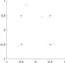
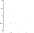
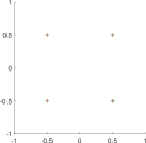
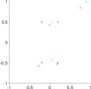
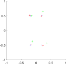
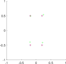
Figure 1 summarizes the experimental results. The three columns correspond to noise levels equal to , , and . Two tests are performed. In the first one (top row), are well-separated from each other. The plots show accurate recovery of the spikes from all values. In the second one (bottom row), the spikes form two nearby pairs. The reconstruction at shows a noticeable error, while the results for and are accurate.
Example 2 (Fourier inversion).
The problem setup is
-
•
.
-
•
.
-
•
are randomly chosen points in .
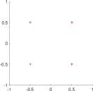
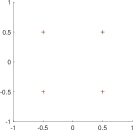

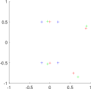
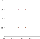
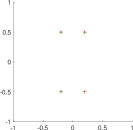
Figure 2 summarizes the experimental results. The three columns correspond to equal to , , and . Two tests are performed. In the first one (top row), are well-separated, and the reconstructions are accurate for all values. In the second one (bottom row), the spikes form two nearby pairs. The reconstruction at shows a noticeable error, but the ones for lower noises are accurate.
4.2. 3D case
In the 3D examples, the Chebyshev grid is , i.e., . The spike weights are set to be and the noises are still Gaussian.
Example 3 (Sparse deconvolution).
The problem setup is
-
•
.
-
•
.
-
•
are random points in outside .

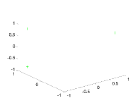

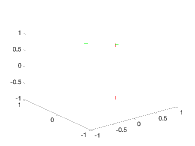
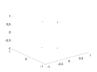
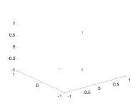
Figure 3 summarizes the experimental results. The three columns correspond to noise levels equal to , , and . Two tests are performed. In the first one (top row), are well-separated from each other. In the second one (bottom row), the spikes form two nearby pairs. The plots show accurate recovery of the spikes from all values in both cases.
Example 4 (Fourier inversion).
The problem setup is
-
•
.
-
•
.
-
•
are randomly chosen points in .
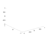


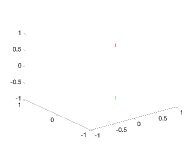

Figure 4 summarizes the experimental results. The three columns correspond to equal to , , and . Two tests are performed. In the first one (top row), and are well-separated from each other. In the second one (bottom row), the spikes again form two nearby pairs. The reconstructions are accurate for all values.
5. Discussions
This note extends the eigenmatrix approach to multidimensional unstructured sparse recovery problems. As a data-driven approach, it assumes no structure on the samples and offers a rather unified framework for such recovery problems. There are several directions for future work.
-
•
A better understanding of the relationship between the size of the Chebyshev grid and the distribution of .
-
•
Also how does the accuracy of the eigenmatrix depend on and the singular value threshold?
-
•
Providing the error estimates for the recovery problems mentioned in Section 1.
-
•
The recovery algorithm presented above follows the ESPRIT algorithm and [andersson2018esprit]. An immediate question is whether other methods (such as the MUSIC and the matrix pencil method) can be extended and combined with the eigenmatrix approach.