A computational method for angle-resolved photoemission spectra from repeated-slab band structure calculations

Abstract

A versatile method for angle-resolved photoemission spectra (ARPES) calculations is reported within the one-step model of photoemission. The initial states are obtained from a repeated-slab calculation using the projector-augmented wave (PAW) method. ARPES final states are constructed by matching the repeated-slab eigenstates of positive energy with free electron states that satisfy the time-reversed low-energy electron diffraction boundary conditions. Nonphysical solutions of the matching equations, which do not respect the flux conservation, are discarded. The method is applied to surface-normal photoemission from graphene as a function of photon energy from threshold up to 100 eV. The results are compared with independently performed multiple scattering calculations and very good agreement is obtained, provided that the photoemission matrix elements are computed with all-electron waves reconstructed from the PAW pseudo-waves. However, if the pseudo-waves are used directly, the relative intensity between $\sigma$- and $\pi$-band emission is wrong by an order of magnitude. The graphene ARPES intensity has a strong photon energy dependence including resonances. The normal emission spectrum from the $\pi$-band shows a hitherto unreported, sharp resonance at a photon energy of 31 eV. The resonance is due to a 2$D$ interband transitions and highlights the importance of matrix element effects beyond the final state plane-wave approximation.

I Introduction

Angle-resolved photoemission spectroscopy (ARPES) is the major experimental method for determining the electronic structure of surfaces and low-dimensional systems, including thin crystalline films and oriented molecules [1]. For two-dimensional systems, the electronic band dispersion $E({\bm{k}}_{\parallel})$ can be fully resolved, where $E$ is the energy and ${\bm{k}}_{\parallel}$ is the 2$D$ crystal momentum. From the ARPES intensity distribution, the wave functions can in principle be reconstructed with the orbital tomography method [2]. In recent years, tremendous progress has been achieved in instrumentation and data acquisition [3], but this is not matched on the theoretical side, where a reliable and flexible calculation method is still missing. To date, accurate ARPES spectra are mostly computed with the multiple scattering method, especially in the layered KKR implementation [4, 5, 6]. While the layered KKR method is efficient and accurate for dense, inorganic matter, applications to open structures such as organic materials have been severely hampered by technical difficulties of full-potential multiple scattering theory [7, 8].

The ground state electronic structure of most materials is well described by density functional theory (DFT) in conjunction with the projector-augmented wave (PAW) method for the solution of the Kohn-Sham equations [9]. In this scheme, surfaces and two-dimensional systems are modeled in the repeated-slab geometry (RSG), i.e. by using periodic boundary conditions in all three dimensions, where adjacent slabs are separated by a sufficient amount of vacuum. While the RSG is being used extensively for the ground state properties of low-dimensional materials, photoemission spectra cannot be obtained directly in this approach, because the periodic boundary conditions of the RSG are incompatible with the photoemission final state, which must evolve into a free electron wave in the asymptotic limit. Therefore the wave functions obtained in RSG must be matched in some way to the far-field solutions which respect the proper boundary conditions. Previously, Kraskovskii et al. [10, 11] have developed an ARPES method based on the RSG and a linearized augmented plane-wave (LAPW) calculation. The method is very accurate for inorganic surfaces with small unit cells, but has not been applied to more complex structures, possibly because of numerical limitations of the LAPW approach [12]. Kobayashi [13] has proposed an ARPES method based on the RSG and PAW method [14], and applied it to low energy spectra of a Bi surface. The approach presented here is conceptually similar to that of Kobayashi [13], but we use a different matching procedure [15] and we go beyond the pseudo-potential level of PAW, by computing the ARPES matrix elements from PAW-reconstructed all-electron wave functions. Moreover, we apply our method to a two-dimensional material and study the photon energy dependence of the spectra, while Ref. [13] was devoted to spin-resolved ARPES from a metallic surface at low photon energy. Let us note that all the approaches above, including the present one, use the one-step model of photoemission which is based on Fermi’s golden rule and a stationary state description of the photoemission final state [4]. ARPES may also be calculated using time-dependent wave-propagation techniques [16, 17]. While such a dynamical approach is mandatory for time-dependent effects observed in ultrafast pumb-probe experiments [18], it appears as an unnecessarily heavy numerical technique for the calculation of time-independent ARPES spectra.

In this paper, we present a theoretical method for ARPES of 2$D$ systems, based on a PAW band structure calculation in RSG. The photoemission final states are obtained by matching the band states above the vacuum level, to free electron waves with the proper, time-reversed LEED boundary conditions. The basic idea of the present matching method was anticipated by Ono and Krüger [15], who studied a one-dimensional toy model. Here we formulate the general theory, develop the computational method and apply it to the prototype 2$D$ material graphene. We focus on the normal-emission ARPES, excited with $p$-polarized light, as a function of photon energy from threshold up to about 100 eV. We find that the ARPES intensity has a strong photon energy dependence including resonances, in agreement with recent experiments [17]. We compare the results with independently performed multiple-scattering calculations and find very good agreement over the whole photon energy range, validating the accuracy of the present approach. The popular final-state plane-wave approximation, in contrast, fails to reproduce the overall energy dependence and misses the resonance effects. We examine the possibility of replacing the all-electron wave functions by PAW pseudo-waves in the calculation of photoemission matrix elements. We conclude that pseudo-waves must not be used, because the intensity ratio between bands of different orbital character (here C-2$s$ and C-2$p_{z}$) can be wrong by one order of magnitude. For normal emission from the graphene $\pi$-band, we predict a sharp Fano-resonance at a photon energy of 31 eV, which has, to the best of our knowledge not been reported before. We show that the resonance is due to the coupling of an evanescent $\sigma$-type 2$D$ band-state with the free-electron continuum.

II General Method

Unless stated otherwise, we use atomic units where $\hbar$=$m_{e}$=$e$=1. We employ the one-step model of photoemission which is based on stationary scattering theory. The photoemission intensity is given by [19]

$$I(\epsilon_{f},\omega,\hat{\bm{p}})\propto\frac{1}{\omega}\sum_{i}\left|\braket{\psi_{f}^{-}}{{\bm{\varepsilon}}\cdot{\hat{\bm{P}}}}{\psi_{i}}\right|^{2}\delta(\epsilon_{i}+\omega-\epsilon_{f})$$ (1)

Here, $\omega$ is the photon energy, $\bm{\varepsilon}$ is the light polarization vector, $\hat{\bm{p}}$ is the direction vector of emitted photoelectron and $\hat{\bm{P}}$ is the electron momentum operator. $\psi_{i}$ is the initial state with energy $\epsilon_{i}$. $\psi_{f}^{-}$ is the photoemission final state with energy $\epsilon_{f}$ where the subscript indicates the time-reversed LEED boundary conditions [19]. For simplicity we disregard the photoelectron spin and assume that there is no absorption. Then the time-reversed LEED state for a photoelectron with momentum ${\bm{p}}$ is the complex conjugate of the LEED state with reversed momentum, i.e.

$$\psi_{f}^{-}=\psi_{-{\bm{p}}}^{*}$$ (2)

Let us consider free-electron eigenstates with momentum ${\bm{p}}=({\bm{p}}_{\parallel},p_{z})$. Their energy is $\epsilon_{\bm{p}}=p^{2}/2$ and the surface parallel crystal momentum is ${\bm{k}}_{\parallel}={\bm{p}}_{\parallel}-{\bm{G}}_{\parallel}$. Here ${\bm{k}}_{\parallel}$ lies in the first surface Brillouin zone and ${\bm{G}}_{\parallel}$ is a surface reciprocal lattice vector. We have $p_{z}=\pm q$ where

$$q\equiv q({\bm{G}}_{\parallel})\equiv\sqrt{p^{2}-\left|{\bm{k}}_{\parallel}+{\bm{G}}_{\parallel}\right|^{2}}$$ (3)

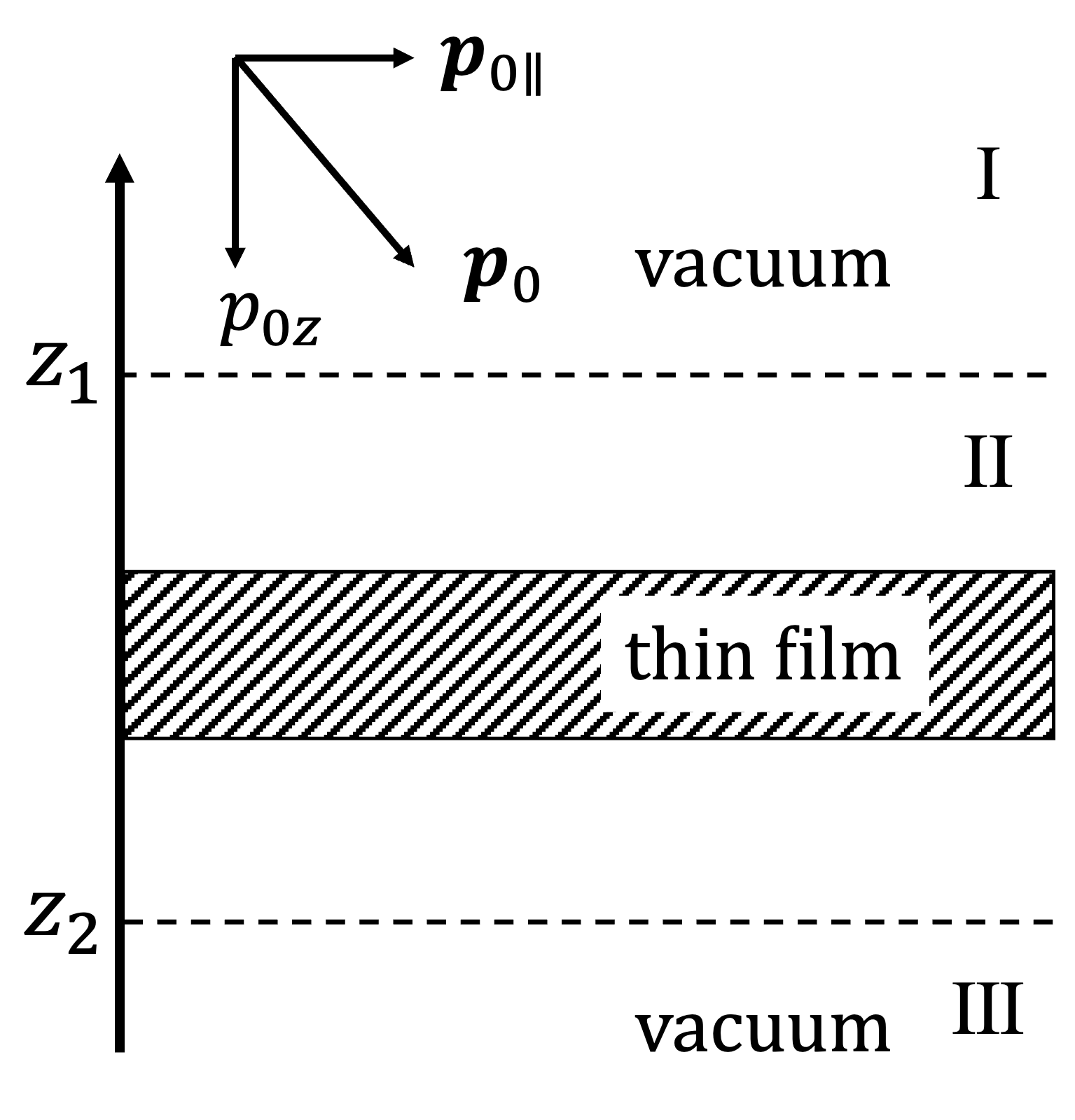
Figure 1: Calculation geometry of LEED state $\psi_{{\bm{p}}_{0}}$.

We divide space in three regions, see Fig.1. Regions I ($z>z_{1}$) and III ($z<z_{2})$ contain only vacuum, while region II ($z_{2}<z<z_{1}$) contains the slab and will be modeled using a supercell of height $c=|z_{2}-z_{1}|$.

We consider a LEED state $\psi_{{\bm{p}}_{0}}$ where an electron with momentum ${\bm{p}}_{0}$ is incident from above (region I in Fig. 1). We have ${\bm{p}}_{0}=({\bm{k}}_{\parallel}+{\bm{G}}_{0\parallel},-q_{0})$, where $q_{0}\equiv q({\bm{G}}_{0\parallel})$. Since the energy and ${\bm{k}}_{\parallel}$ are conserved, the wave function in the vacuum regions can be written as a linear combination of plane waves with momentum ${\bm{p}}=({\bm{k}}_{\parallel}+{\bm{G}}_{\parallel},\pm q)$, where $+q$ and $-q$ correspond to regions I and III, respectively and $p=p_{0}$ is fixed. Thus we can write the LEED wave as

$$\psi_{\rm I}({\bm{r}})=e^{i{\bm{k}}_{\parallel}\cdot{\bm{r}}_{\parallel}}\left(e^{i{\bm{G}}_{0\parallel}\cdot{\bm{r}}_{\parallel}-iq_{0}z}+\sum_{{\bm{G}}_{\parallel}}R_{{\bm{G}}_{\parallel}}e^{i{\bm{G}}_{\parallel}\cdot{\bm{r}}_{\parallel}+iqz}\right)$$ (4)

$$\psi_{\rm I\!I\!I}({\bm{r}})=e^{i{\bm{k}}_{\parallel}\cdot{\bm{r}}_{\parallel}}\sum_{{\bm{G}}_{\parallel}}T_{{\bm{G}}_{\parallel}}e^{i{\bm{G}}_{\parallel}\cdot{\bm{r}}_{\parallel}-iqz}$$ (5)

Here the sums over ${\bm{G}}_{\parallel}$ are restricted by $|{\bm{k}}_{\parallel}+{\bm{G}}_{\parallel}|\leq p_{0}$, and $R_{{\bm{G}}_{\parallel}}$, $T_{{\bm{G}}_{\parallel}}$ are complex coefficients. In region II we develop the LEED wave over eigenstates of the RSG calculation, i.e. Bloch waves $\varphi_{n{\bm{k}}}$ with energy $\epsilon_{n{\bm{k}}}$, where ${\bm{k}}=({\bm{k}}_{\parallel},k_{z})$ and $n$ is a band index. The states $\varphi_{n{\bm{k}}}$ are taken to be normalized in the supercell volume. Upon introducing the 3$D$-cell periodic functions,

$$u_{n{\bm{k}}}({\bm{r}})=\varphi_{n{\bm{k}}}({\bm{r}})e^{-i{\bm{k}}\cdot{\bm{r}}}$$ (6)

we may write

$$\psi_{\rm I\!I}({\bm{r}})=e^{i{\bm{k}}_{\parallel}\cdot{\bm{r}}_{\parallel}}\sum_{n,k_{z}}^{\prime}c_{nk_{z}}u_{n{\bm{k}}}({\bm{r}})e^{ik_{z}z}$$ (7)

Here $c_{nk_{z}}$ are complex coefficients and the primed sum means that we include only eigenstates that approximately respect energy conservation, i.e. $\epsilon_{n{\bm{k}}}\approx\epsilon_{{\bm{p}}_{0}}$. The coefficients $c_{nk_{z}}$, $R_{{\bm{G}}_{\parallel}}$ and $T_{{\bm{G}}_{\parallel}}$ are determined by the condition that the wave function and its gradient be continuous at the boundary surfaces, i.e. at all points (${\bm{r}}_{\parallel},z_{1})$ and $({\bm{r}}_{\parallel},z_{2})$. These conditions are more conveniently applied in reciprocal space. For a 2$D$-cell periodic functions $f({\bm{r}}_{\parallel})$, we define the lattice Fourier transform as

$$f({\bm{r}}_{\parallel}) = \sum_{{\bm{G}}_{\parallel}}{\bar{f}}_{{\bm{G}}_{\parallel}}e^{i{\bm{G}}_{\parallel}\cdot{\bm{r}}_{\parallel}}$$ (8)

$${\bar{f}}_{{\bm{G}}_{\parallel}} = \frac{1}{A}\iint_{A}d{\bm{r}}_{\parallel}f({\bm{r}}_{\parallel})e^{-i{\bm{G}}_{\parallel}\cdot{\bm{r}}_{\parallel}}$$ (9)

where the integral is over the 2$D$ unit cell with area $A$. We have

$$u_{n{\bm{k}}}({\bm{r}}_{\parallel},z)=\sum_{{\bm{G}}_{\parallel}}{\bar{u}}_{n{\bm{k}};{\bm{G}}_{\parallel}}(z)e^{i{\bm{G}}_{\parallel}\cdot{\bm{r}}_{\parallel}}$$ (10)

From Eqs (4)(5)(7) together with the orthogonality of the functions $e^{i{\bm{G}}_{\parallel}\cdot{\bm{r}}_{\parallel}}$, it is easy to see that the continuity of $\psi$ across the region boundaries requires that

$$R_{{\bm{G}}_{\parallel}}e^{iqz_{1}} + \delta_{{\bm{G}}_{\parallel},{\bm{G}}_{0\parallel}}e^{-iq_{0}z_{1}}$$ (11)

$$= \sum_{n,k_{z}}^{\prime}c_{nk_{z}}{\bar{u}}_{n{\bm{k}};{\bm{G}}_{\parallel}}(z_{1})e^{ik_{z}z_{1}}$$

$$T_{{\bm{G}}_{\parallel}}e^{-iqz_{2}} = \sum_{n,k_{z}}^{\prime}c_{nk_{z}}{\bar{u}}_{n{\bm{k}};{\bm{G}}_{\parallel}}(z_{2})e^{ik_{z}z_{2}}$$ (12)

where $q=q({\bm{G}}_{\parallel})$ is given by Eq. (3). From the continuity of $\partial\psi/\partial z$ we obtain

$$R_{{\bm{G}}_{\parallel}}qe^{iqz_{1}} - \delta_{{\bm{G}}_{\parallel},{\bm{G}}_{0\parallel}}qe^{-iq_{0}z_{1}}$$ (13)

$$= \sum_{n,k_{z}}^{\prime}c_{nk_{z}}{\bar{u}}_{n{\bm{k}};{\bm{G}}_{\parallel}}(z_{1})k_{z}e^{ik_{z}z_{1}}$$

$$-T_{{\bm{G}}_{\parallel}}qe^{-iqz_{2}} = \sum_{n,k_{z}}^{\prime}c_{nk_{z}}{\bar{u}}_{n{\bm{k}};{\bm{G}}_{\parallel}}(z_{2})k_{z}e^{ik_{z}z_{2}}$$ (14)

We refer to Eqs (11–14) as the matching equations. Note that $R_{{\bm{G}}_{\parallel}}=T_{{\bm{G}}_{\parallel}}=0$ for all ${\bm{G}}_{\parallel}$ with $|{\bm{k}}_{\parallel}+{\bm{G}}_{\parallel}|>p_{0}$. For exact matching, these equations must hold simultaneously for all ${\bm{G}}_{\parallel}$, which leads to an over-determined, infinite dimensional linear problem for the unknown coefficients, namely the $c_{nk_{z}}$, and the $T_{{\bm{G}}_{\parallel}}$, $R_{{\bm{G}}_{\parallel}}$ for $|{\bm{k}}_{\parallel}+{\bm{G}}_{\parallel}|<p_{0}$. In practice, we retain a finite number of equations for ${\bm{G}}_{\parallel}$ vectors below some cut-off kinetic energy and find the least squares solution of the over-determined system. When a plane wave basis set is used for the RSG calculation, we have $u_{n{\bm{k}}}({\bm{r}})=\sum_{\bm{G}}C^{n{\bm{k}}}_{\bm{G}}e^{i{\bm{G}}\cdot{\bm{r}}}$ and ${\bar{u}}_{n{\bm{k}};{\bm{G}}_{\parallel}}(z)=\sum_{G_{z}}C^{n{\bm{k}}}_{\bm{G}}e^{iG_{z}z}$ where $C^{n{\bm{k}}}_{\bm{G}}$ are the usual plane wave coefficients. The matrix elements in Eq. (1) are evaluated with all-electron wave functions $\varphi_{n{\bm{k}}}({\bm{r}})$ or, for comparison, with pseudo wave functions $\tilde{\varphi}_{n{\bm{k}}}({\bm{r}})$, see the S.M. for details [20]. We use the Vienna ab initio simulation package (VASP) [21] for the RSG calculation and the VaspUnfolding program [22] for the reconstruction of the all-electron functions from the PAW pseudo functions [14]. Note that for the matching problem, Eqs.(11)–(14), all-electron functions are not needed, since the matching is done at $z=z_{1,2}$, outside any PAW augmentation sphere, where $\tilde{\varphi}_{n{\bm{k}}}({\bm{r}})=\varphi_{n{\bm{k}}}({\bm{r}})$.

III Application to graphene

In this section, we apply the method to photoemission from an isolated graphene sheet, and we study the normal photoemission intensity as function of photon energy for different initial bands. First, we calculate the LEED state $\psi_{{\bm{p}}_{0}}$ with ${\bm{p}}_{0}=(0,0,p_{0z})$ for $p_{0z}=-\sqrt{2\epsilon_{f}}$ and then the photoemission matrix element Eq. (1) with the time-reversed LEED state Eq. (2).

III.1 Density functional theory calculation

We compute the photoemission initial states $\psi_{i}$ and the high energy band states $\varphi_{n{\bm{k}}}$ of Eq. (6) in RSG using the PAW code VASP [21]. The supercell lattice parameters are $a=2.44$ Å, $c=20$ Å. We use a plane-wave cut-off energy of $400$ eV and a 9$\times$9 $k_{\parallel}$-mesh for the 2$D$ Brillouin zone sampling. Theses are typical settings for a DFT ground state calculation. What differs from a usual RSG ground state calculation, is that we use a fine $k_{z}$ point mesh with 120 points and need to compute enough bands up to the wanted photoemission energy. For the matching equations (11)-(14), 400 ${\bm{G}}_{\parallel}$ points are used. Figure 2 shows the band structure along $k_{z}$ at ${\bm{k}}_{\parallel}$=(0,0). Here and in the following $E$ denotes the electron energy measured from the vacuum level. The computed work function is 4.21 eV.

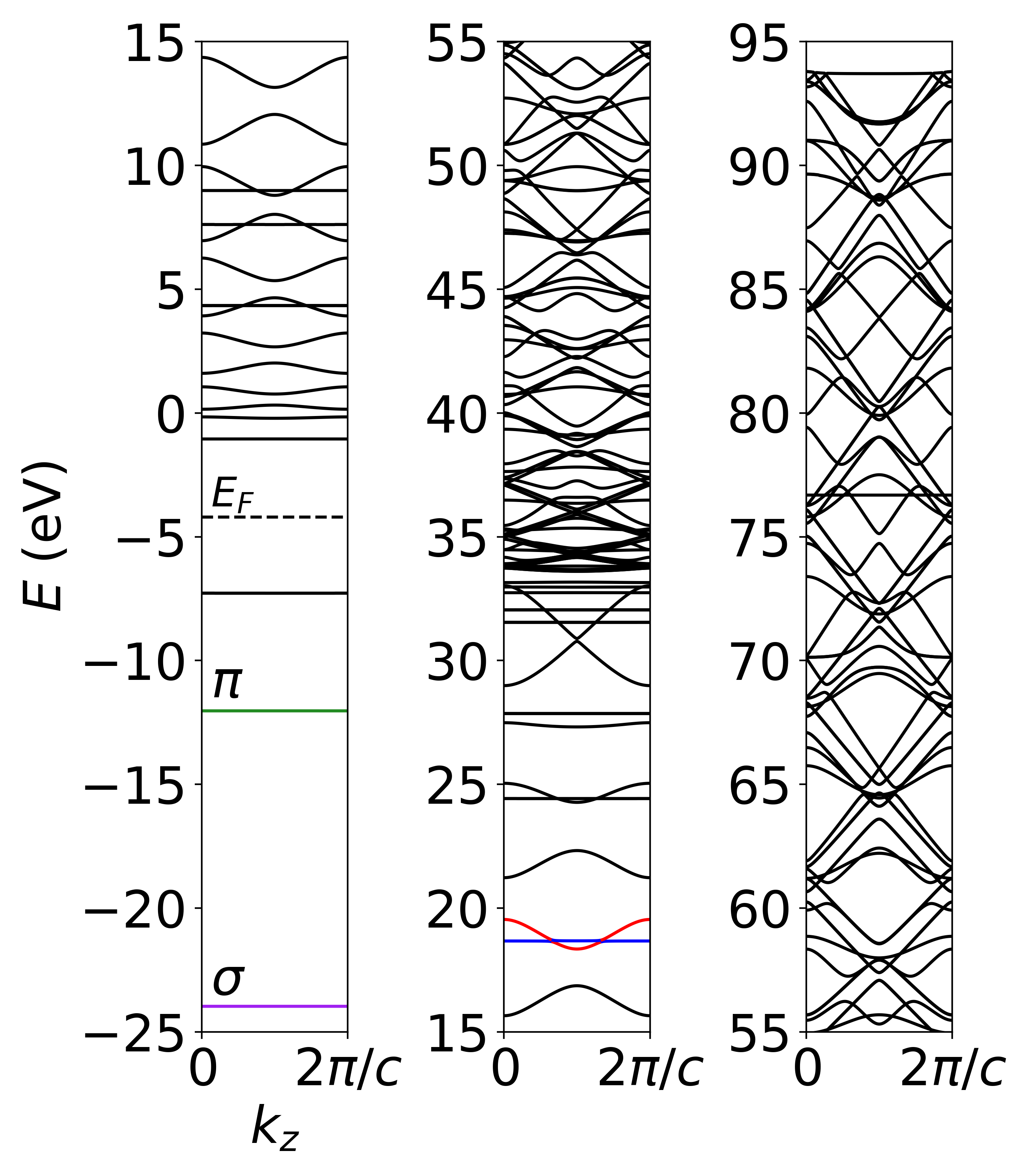
Figure 2: $k_{z}$ band dispersion for ${\bm{k}}_{\parallel}=(0,0)$. $E$ is the energy measured from the vacuum level. $c$ is the supercell dimension (20 Å). The black dashed line indicates Fermi energy ($E_{F}$). $\sigma$ and $\pi$ bands are colored purple and green, respectively. Flat and dispersive energy bands around 19 eV are colored blue and red, respectively.

III.2 Construction of LEED states

In a calculation using RSG, some eigenstates $\varphi_{n{\bm{k}}}$ with positive energy are evanescent and do not propagate along $z$. Such states do not contribute to the photoemission process and must be discarded [13]. To identify these states, we compute the probability current along $z$, which is given by

$$J_{z,m}=\iint_{A}d{\bm{r}}_{\parallel}\operatorname{Im}\left[{\varphi}_{m}^{*}\frac{\partial}{\partial z}{\varphi}_{m}\right]$$ (15)

where $m=n{\bm{k}}$ and $\varphi_{m}({\bm{r}})$ is evaluated at $z=z_{1}$. Details of the flux calculation are given in section II of the S.M. [20]. We keep only states $\varphi_{n{\bm{k}}}$ whose flux exceeds some numerical threshold. Here we take $|J_{z,m}|>3\times 10^{-5}$ [a.u.]. For constructing a photoemission final state of energy $\epsilon_{f}$ one would ideally use only band states with exactly the same energy, $\epsilon_{n{\bm{k}}}=\epsilon_{f}$. However, for numerical reasons, such as the discretization of $k_{z}$ space, we need to slightly relax this constraint and solve the matching equations with band states $\varphi_{n{\bm{k}}_{\parallel}}$ in a small interval around the exact energy $\epsilon_{f}$. Here we use $|\epsilon_{n{\bm{k}}}-\epsilon_{f}|<0.01$ eV.

Some numerical solutions of the matching equations do not correspond to physical scattering states. Acceptable LEED states satisfy the probability conservation

$${\cal T}+{\cal R}=1,$$ (16)

where ${\cal T}$ and ${\cal R}$ are the total transmission and reflection coefficients, respectively. Solutions that do not satisfy Eq. (16) are discarded. For the 2$D$ system we have

$${\cal T} = {\cal T}_{0}+{\cal T}_{\neq 0},$$

$${\cal T}_{0} = |T_{{\bm{G}}_{0\parallel}}|^{2},\quad{\cal T}_{\neq 0}=\sum_{{\bm{G}}_{\parallel}(\neq{\bm{G}}_{0\parallel})}\frac{q({\bm{G}}_{\parallel})}{q_{0}}|T_{{\bm{G}}_{\parallel}}|^{2},$$

$${\cal R} = {\cal R}_{0}+{\cal R}_{\neq 0},$$

$${\cal R}_{0} = |R_{{\bm{G}}_{0\parallel}}|^{2},\quad{\cal R}_{0}=\sum_{{\bm{G}}_{\parallel}(\neq{\bm{G}}_{0\parallel})}\frac{q({\bm{G}}_{\parallel})}{q_{0}}|R_{{\bm{G}}_{\parallel}}|^{2}.$$ (17)

with $q({\bm{G}}_{\parallel})$ defined in Eq. (3) and $q_{0}\equiv q({\bm{G}}_{0\parallel})$. To enforce the probability conservation numerically, we exclude all states with $|{\cal T}+{\cal R}-1|>\eta$, where $\eta=0.05$ in the present case. For larger supercell sizes, smaller $\eta$ values can be used as we have checked.

The transmission and reflection coefficients are shown in Fig. 3, where the ${\bm{G}}_{\parallel}=0$ components and the ${\bm{G}}_{\parallel}\neq 0$ components are plotted separately in order to illustrate the effect of umklapp scattering (${\bm{G}}\neq 0$). Umklapp scattering is possible for $E>{\bm{b}}_{1}^{2}/2=8\pi^{2}/3a^{2}=33.7$ eV, indicated by a dotted line in Fig. 3. Above this energy, direct and umklapp components of the reflectivity are of about equal intensity, while in transmission, umklapp scattering strongly dominates for energies around 80 eV. The energy dependence of the total transmission coefficient agrees well with Ref. [23].

For some energies, acceptable LEED states cannot be found. As a result, the plots in Fig. 3 are not continuous, i.e. there are small gaps in the energy mesh. The main reason for this is that the band structure $\epsilon(k_{z})$ (Fig. 2) has gaps which are due to the artificial periodicity in the RSG along the $c$ axis. If the photoelectron energy falls into a gap, the ARPES result can be obtained by interpolating between two nearby energy points. If interpolation is deemed not accurate enough, then one should perform a new RSG calculation with a somewhat different supercell lattice constant $c^{\prime}$. As it is well known from the Kronig-Penney model [24], a change in lattice constant shifts the energy gaps in the band structure, and $c^{\prime}$ can be tuned to obtain a solution for the desired energy. This is shown in the S.M. [20] where results for a twice larger supercell ($c^{\prime}=40$ Å) are presented.

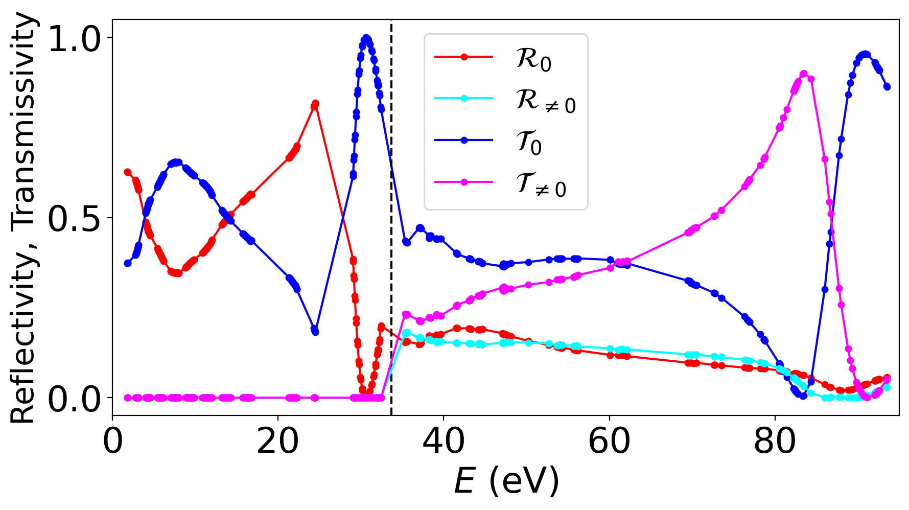
Figure 3: Reflection and transmission coefficients of the calculated LEED states, decomposed into ${\bm{G}}_{\parallel}={\bm{G}}_{0\parallel}$ and ${\bm{G}}_{\parallel}\neq{\bm{G}}_{0\parallel}$ components (umklapp scattering). The dashed line indicates the theoretical onset of umklapp scattering ($E=33.7$ eV). The curves are ${\cal R}_{0}$ (red), ${\cal R}_{\neq 0}$ (cyan), ${\cal T}_{0}$ (blue) and ${\cal T}_{\neq 0}$ (magenta).

As an example of the LEED wave functions obtained with the present method, Fig. 4(a) shows the all-electron wave $\psi_{{\bm{p}}_{0}}$ and the corresponding pseudo wave $\tilde{\psi}_{{\bm{p}}_{0}}$ for $\epsilon_{f}=14$ eV. Matching was performed at $z_{1}=10$ Å and $z_{2}=-10$ Å (black dashed line). The obtained wave functions are smooth at these points. From the behavior of the wave function in Fig. 4(a) it is clear that the precise choice of the matching points is not important. Smooth matching can be achieved for wide range of values, typically $|z_{1,2}|>5$ Å.

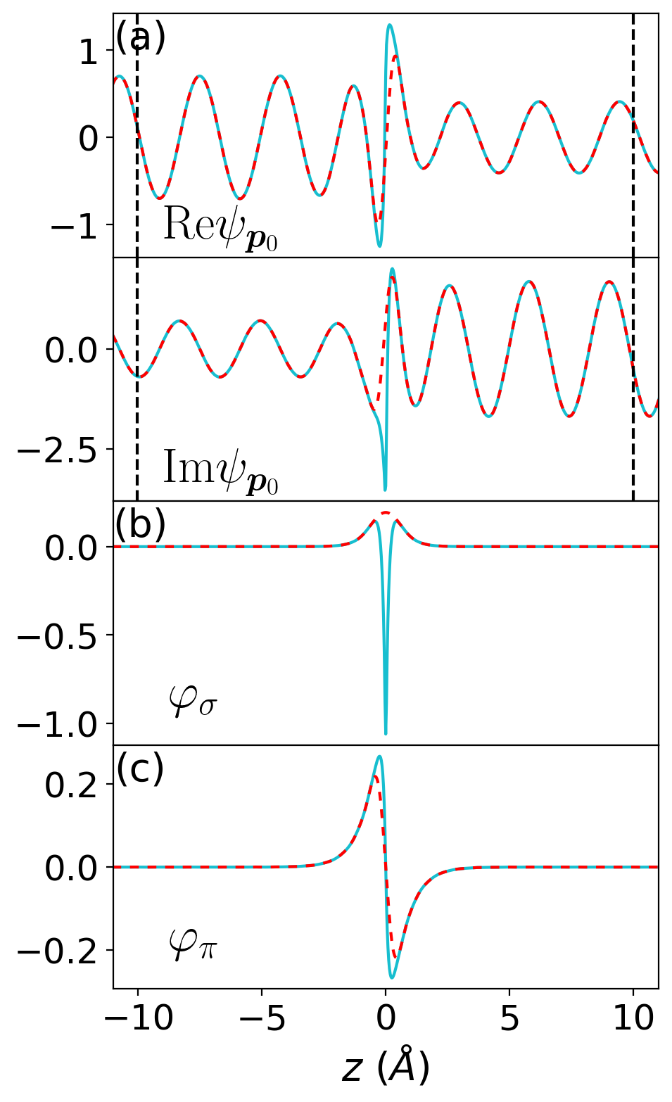
Figure 4: Wave function line plots. The lines are along $z$ and cross the center of a C atom at $z=0$. All-electron waves are shown as cyan solid lines and pseudo waves as red dashed lines. (a) LEED state at kinetic energy $E=14$ eV, (b) $\sigma$ initial state and (c) $\pi$ initial state. The wave amplitudes are given in units of 1 in (a) and in a.u. in (b,c).

III.3 Photoemission intensity calculation

We have calculated the energy dependence of the normal photoemission intensity emitted from graphene with linear $z$-polarized light, i.e. using Eq. (1) with ${\bm{A}}={\hat{\bm{e}}}_{z}$. Because of ${\bm{k}}_{\parallel}$ conservation, we only probe the $\Gamma$ point in the 2$D$ Brillouin zone. Among the four valence bands of graphene [25], only two have non-zero normal emission intensity for this polarization, namely the lowest $\sigma$ band of C-2$s$ orbital character and the $\pi$-band of C-2$p_{z}$ character, which we refer to as $\sigma$ and $\pi$ in the following. Their energy levels are indicated by purple and green lines in Fig. 2 and wave function plots are displayed in Fig. 4(b,c).

Figure 5(a) shows the photoemission intensity for the $\sigma$ and $\pi$ initial states, as a function of photoelectron kinetic energy $E$. In both cases, the photoemission intensity has a pronounced energy dependence including resonances. For the $\sigma$ initial state, the photoemission intensity grows slowly with energy from threshold to 85 eV, except for some oscillations between 24 eV and 35 eV. Since the photoemission final state has time-reversed LEED boundary conditions, peculiar features of the LEED energy dependence may also show up in the photoemission spectrum. We observe that the $\sigma$ photoemission spectral shape resembles the reflectivity for energies below the on-set of umklapp scattering (33.7 eV) and the transmissivity for higher energies, see Fig. 3. The peak-dip structures in the LEED reflectivity, around 24–32 eV and 33–35 eV, were explained by Nazarov et al. [23] as being caused by resonances in the graphene band structure and the onset of the umklapp scattering.

The $\pi$ initial state has a very different energy dependence than the $\sigma$ state. After a rise at threshold, the intensity mostly decreases from 6 eV to 87 eV. Interestingly there is a very sharp resonance at $E=19$ eV (i.e. at photon energy $31$ eV) which has, to the best of our knowledge, not been reported so far. The resonance is unrelated to the reflectivity (Fig. 3). We have analyzed the final state waves in the RSG calculation at the 2$D$ $\Gamma$-point. The 19 eV resonance corresponds to the lowest energy ${\bm{k}}_{\parallel}=0$ state that is both evanescent and dipole-transition allowed from the $\pi$ initial state. The energy level of this state is marked in blue in Fig. 2. The wave function is evanescent as seen by the absence of $k_{z}$ dispersion. It has the same point symmetry as the $\sigma$ initial state (fully symmetric $a_{1g}$) with a large amplitude inside the C₆ rings, rather than on the C-atoms, see the S.M. [20]. A plane-wave-like state propagating in $+z$-direction of the same energy (the red band in Fig. 2) has a small overlap with the evanescent state. This leads a wave function mixing and, as we have checked, to an avoided crossing of the two bands. (The gap opening is so small that it cannot be seen on the scale of Fig. 2.) The weak coupling between the evanescent state and the free-electron-like continuum states produces the sharp Fano-like resonance in the $\pi$-band photoemission, seen in Fig. 5(a) at $E=19$ eV.

In Fig. 5(b) we compare the ARPES intensity of the $\sigma$ state obtained with the present (“matching”) method with two independent theoretical methods, namely real-space multiple scattering (MS) [26, 25] and the final state plane-wave (FSPW) approximation. We note that the real-space MS has been shown to be a reliable method for ARPES calculations of various system, including oriented molecules [27], metal surfaces [26] and graphite [25]. The energy dependence of “matching” and “MS” is very similar, which proves the validity of the present matching approach. The MS calculation shows small differences, namely a generally more smooth energy dependence and the absence of a peak at 33.7 eV (dashed vertical line). Both differences can be attributed to approximations used in the real-space MS method [26], namely the finite-cluster approximation which broadens the band features, and the simple model used for the surface barrier, which fails to reproduce the “purely structural” LEED resonance at the on-set of umklapp scattering [23]. Apart from these details, the overall agreement between “matching” and “MS” is very good and it is even better for the $\pi$ initial state [Fig. 5(c)]. Note that in Fig. 5(b) and 5(c), we used the same intensity scaling for “matching” and “MS”. It follows that not only the spectral shapes but also the relative intensity between $\sigma$ and $\pi$ agrees between “matching” and “MS”. The FSPW on the other hand, gives very poor results, see blue curves in Fig. 5(b) and 5(c). For the $\sigma$-band, the energy dependence is totally wrong. For the $\pi$ band, the overall dependence is better, but the resonance at 19 eV and the minimum at 85 eV are missing. We conclude that the FSPW approximation is unreliable for the photon energy dependence of ARPES, confirming other recent literature [15, 17, 16].

III.4 Comparison of pseudo and all-electron wave function

In the calculation of Fig. 5(a), we used all-electron wave functions for both initial and final states in the photoemission intensity calculations. Here, we discuss the question whether we all-electron wave functions can be replaced with pseudo wave functions.

In Figure 6(a,b), we compare four types of calculation by choosing either the all-electron (“ae”) or the pseudo (“ps”) wave function for the initial and the final state. The overall energy dependence is similar between the four calculation schemes but there are also important differences. This is particularly true for the $\sigma$ initial state, Fig. 6(a). When replacing the all-electron wave with a pseudo-wave in the final state, the photoemission intensity may change by up to 30%. When the pseudo wave is used in for the initial state, then the intensity is reduced by one order of magnitude as compared to the all-electron calculation (note the scaling factor $\times 15$ used in the plot). Moreover, the energy dependence is very different for $E<20$ eV.

The differences are smaller for the $\pi$ initial state, Fig. 6(b). Replacing the all-electron initial state wave by the pseudo wave hardly changes the intensity for $E<60$ eV, although some changes are seen for higher energy. If the all-electron functions are replaced by pseudo functions in the final state, the photoemission intensity is reduced by about 20% for $E<80$ eV and strongly increased for $E>85$ eV. The reason why the choice between all-electron and pseudo function has a much larger effect for the $\sigma$ band than for the $\pi$ band, is obvious when looking at the wave function plots in Fig. 4(b,c). The $\sigma$ pseudo wave has no node, while the all-electron wave has the node of the C-2$s$ atomic wave.

Looking at the similar spectral shapes of Fig6(a,b) one might think that using pseudo wave functions can be an acceptable approximation when total intensities are not relevant. However, this is misleading because here we have considered only the $\Gamma$-point, where C-$2s$ and C-$2p$ orbitals cannot mix by symmetry. For a general ${\bm{k}}_{\parallel}$-point, the $\sigma$ band contains C-$2s$ and C-$2p_{xy}$ components. Since the $2s$ pseudo-wave leads to a dramatic decrease of intensity but the $2p$ pseudo-wave does not, there is no way to rescale the pseudo-wave intensity to match the correct all-electron intensity. We conclude that, in general, all-electron wave functions must be used for a reliable photoemission intensity calculation. A possible exception might be the $\pi$-states of graphene and flat organic molecules [2], as these states are of purely C-$p$ character.

(a)

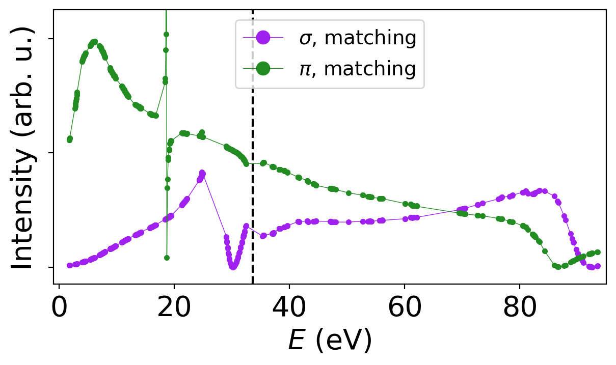
(b)

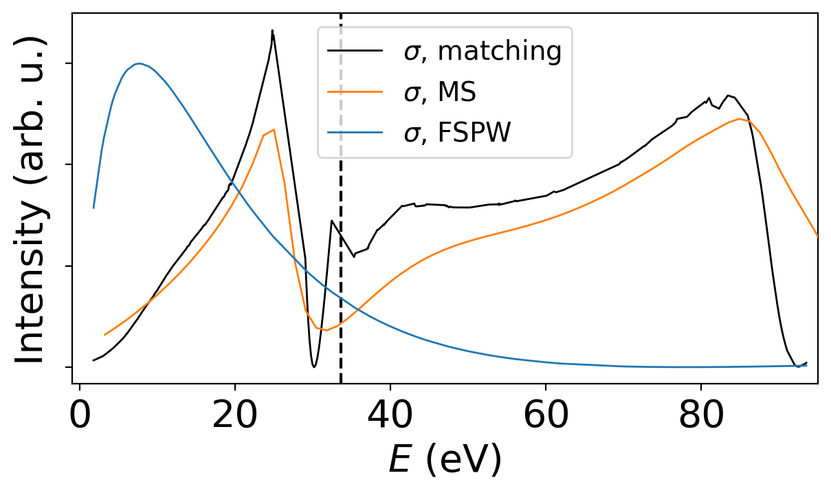
(c)

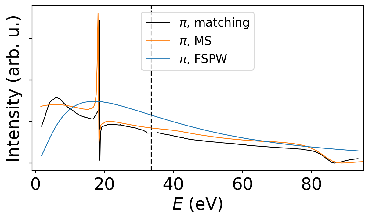
Figure 5: (a) Normal emission intensity from the graphene $\sigma$ and $\pi$ bands obtained with the present “matching” method as a function of kinetic energy $E$. (b,c) Comparison with a multiple scattering calculation (MS), and the final state plane wave approximation (FSPW). In (b) and (c), the calculated intensities are arbitrarily scaled keeping the ratio of $\sigma$ and $\pi$ intensities within each method.

(a)

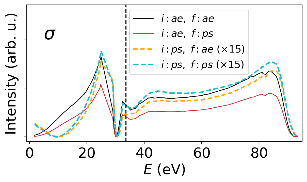
(b)

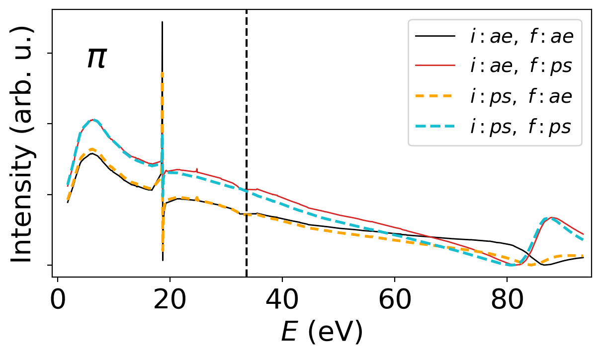
Figure 6: Comparison between all-electron (ae) and pseudo (ps) wave functions for initial (i) and final (f) states, in the matching method calculation of normal photoemission from graphene. (a) $\sigma$ initial state. (b) $\pi$ initial state. Note that the intensity of the (i:ps) spectra in (a) are multiplied by a factor 15.

IV Conclusions

In summary, we have developed a flexible and accurate computational method for ARPES from 2$D$ systems. The photoemission final states are obtained by matching Bloch waves of a DFT calculation in repeated-slab-geometry with free waves having the proper time-reversed LEED boundary conditions. The DFT calculation is performed in the PAW method with a standard code. The method has been applied to ARPES from a graphene monolayer. The results were compared with independently performed multiple scattering calculations [25] and very good agreement was obtained in all cases. The closely related LEED reflectivity spectrum was also checked against the theoretical literature [10]. In the PAW method, transition matrix elements can be calculated either with PAW pseudo-waves or with reconstructed all-electron waves. The comparison shows that all-electron waves must be used for obtaining reliable ARPES intensities. We have studied the energy dependence of the normal emission intensity from the graphene $\sigma$ and $\pi$ bands in the kinetic energy range 0–95 eV. For both bands, we find a pronounced energy dependence with resonances. We predict a sharp Fano resonance for $\pi$-band normal emission at a kinetic energy around 19 eV, due to a strong 2$D$ interband transition which is weakly coupled to a free-electron-like final state.

References

- Damascelli et al. [2003] A. Damascelli, Z. Hussain, and Z.-X. Shen, Angle-resolved photoemission studies of the cuprate superconductors, Rev. Mod. Phys. 75, 473 (2003).
- Puschnig et al. [2009] P. Puschnig, S. Berkebile, A. J. Fleming, G. Koller, K. Emtsev, T. Seyller, J. D. Riley, C. Ambrosch-Draxl, F. P. Netzer, and M. G. Ramsey, Reconstruction of Molecular Orbital Densities from Photoemission Data, Science 326, 702 (2009).
- Tusche et al. [2019] C. Tusche, Y.-J. Chen, C. M. Schneider, and J. Kirschner, Imaging properties of hemispherical electrostatic energy analyzers for high resolution momentum microscopy, Ultramicroscopy 206, 112815 (2019).
- Pendry [1976] J. Pendry, Theory of photoemission, Surface Science 57, 679 (1976).
- Braun [1996] J. Braun, The theory of angle-resolved ultraviolet photoemission and its applications to ordered materials, Reports on Progress in Physics 59, 1267 (1996).
- Ono et al. [2021] R. Ono, A. Marmodoro, J. Schusser, Y. Nakata, E. F. Schwier, J. Braun, H. Ebert, J. Minár, K. Sakamoto, and P. Krüger, Surface band characters of the weyl semimetal candidate material revealed by one-step angle-resolved photoemission theory, Phys. Rev. B 103, 125139 (2021).
- Antonios Gonis [2000] W. H. B. Antonios Gonis, Multiple Scattering in Solids, 1st ed., Graduate Texts in Contemporary Physics (Springer-Verlag, New York, 2000).
- Hatada et al. [2007] K. Hatada, K. Hayakawa, M. Benfatto, and C. R. Natoli, Full-potential multiple scattering for x-ray spectroscopies, Phys. Rev. B 76, 060102 (2007).
- Blöchl [1994] P. E. Blöchl, Projector augmented-wave method, Phys. Rev. B 50, 17953 (1994).
- Krasovskii [2004] E. E. Krasovskii, Augmented-plane-wave approach to scattering of Bloch electrons by an interface, Phys. Rev. B 70, 245322 (2004).
- Krasovskii [2021] E. Krasovskii, Ab Initio Theory of Photoemission from Graphene, Nanomaterials 11, 10.3390/nano11051212 (2021).
- Krasovskii [2020] E. E. Krasovskii, Character of the outgoing wave in soft x-ray photoemission, Phys. Rev. B 102, 245139 (2020).
- Kobayashi [2020] K. Kobayashi, Method of forming time-reversed LEED states from repeated-slab calculations, Journal of Physics: Condensed Matter 32, 495002 (2020).
- Kresse and Joubert [1999] G. Kresse and D. Joubert, From ultrasoft pseudopotentials to the projector augmented-wave method, Phys. Rev. B 59, 1758 (1999).
- Ono and Krüger [2018] R. Ono and P. Krüger, A One-Dimensional Model for Photoemission Calculations from Plane-Wave Band Structure Codes, e-Journal of Surface Science and Nanotechnology 16, 49 (2018).
- Dauth et al. [2016] M. Dauth, M. Graus, I. Schelter, M. Wießner, A. Schöll, F. Reinert, and S. Kümmel, Perpendicular Emission, Dichroism, and Energy Dependence in Angle-Resolved Photoemission: The Importance of The Final State, Phys. Rev. Lett. 117, 183001 (2016).
- Kern et al. [2023] C. S. Kern, A. Haags, L. Egger, X. Yang, H. Kirschner, S. Wolff, T. Seyller, A. Gottwald, M. Richter, U. De Giovannini, A. Rubio, M. G. Ramsey, F. m. c. C. Bocquet, S. Soubatch, F. S. Tautz, P. Puschnig, and S. Moser, Simple extension of the plane-wave final state in photoemission: Bringing understanding to the photon-energy dependence of two-dimensional materials, Phys. Rev. Res. 5, 033075 (2023).
- Kasmi et al. [2017] L. Kasmi, M. Lucchini, L. Castiglioni, P. Kliuiev, J. Osterwalder, M. Hengsberger, L. Gallmann, P. Krüger, and U. Keller, Effective mass effect in attosecond electron transport, Optica 4, 1492 (2017).
- Brown et al. [1980] E. R. Brown, S. L. Carter, and H. P. Kelly, Photoionization cross section and resonance structure of ClI, Phys. Rev. A 21, 1237 (1980).
- [20] See Supplemental Material at …for details about (I) the calculation of the photoemission matrix elements, (II) the probability current , (III) results obtained with a larger supercell size Å and (IV) the wave function character at the resonance energy eV.
- Kresse and Furthmüller [1996] G. Kresse and J. Furthmüller, Efficient iterative schemes for ab initio total-energy calculations using a plane-wave basis set, Phys. Rev. B 54, 11169 (1996).
- [22] https://github.com/QijingZheng/VaspBandUnfolding.
- Nazarov et al. [2013] V. U. Nazarov, E. E. Krasovskii, and V. M. Silkin, Scattering resonances in two-dimensional crystals with application to graphene, Phys. Rev. B 87, 041405 (2013).
- Ashcroft and Mermin [1976] N. W. Ashcroft and N. D. Mermin, Solid State Physics (Saunders College, Philadelphia, 1976).
- Krüger and Matsui [2022] P. Krüger and F. Matsui, Observation and theory of strong circular dichroism in angle-revolved photoemission from graphite, Journal of Electron Spectroscopy and Related Phenomena 258, 147219 (2022).
- Krüger et al. [2011] P. Krüger, F. Da Pieve, and J. Osterwalder, Real-space multiple scattering method for angle-resolved photoemission and valence-band photoelectron diffraction and its application to Cu(111), Phys. Rev. B 83, 115437 (2011).
- Krüger [2018] P. Krüger, Photoelectron Diffraction from Valence States of Oriented Molecules, Journal of the Physical Society of Japan 87, 061007 (2018).