DeepDRK: Deep Dependency Regularized Knockoff for Feature Selection
Abstract
Model-X knockoff, among various feature selection methods, received much attention recently due to its guarantee on false discovery rate (FDR) control. Subsequent to its introduction in parametric design, knockoff is advanced to handle arbitrary data distributions using deep learning-based generative modeling. However, we observed that current implementations of the deep Model-X knockoff framework exhibit limitations. Notably, the “swap property" that knockoffs necessitate frequently encounter challenges on sample level, leading to a diminished selection power. To overcome, we develop “Deep Dependency Regularized Knockoff (DeepDRK) 111The “DeepDRK” term is pronounced as “Deep Dark” and is inspired by the underground cave biome prevalent in the world of Minecraft, whereas the proposed feature selection model acts as the guiding beacon amidst the darkness of unknown.", a distribution-free deep learning method that strikes a balance between FDR and power. In DeepDRK, a generative model grounded in a transformer architecture is introduced to better achieve the “swap property". Novel efficient regularization techniques are also proposed to reach higher power. Our model outperforms other benchmarks in synthetic, semi-synthetic, and real-world data, especially when sample size is small and data distribution is complex.
Keywords Feature Selection, Deep Learning, Model-X Knockoff, FDR Control
1 Introduction
Feature selection (FS) has drawn tremendous attention over the past decades, due to rapidly increasing data dimension [22]. Still, perfectly locating informative features is deemed mission impossible [56]. It is hence necessary to devise algorithms to select features with controlled error rates.
Targeting this goal, Model-X knockoffs, a novel framework, is proposed in [5, 12] to select relevant features while controlling the false discovery rate (FDR). In contrast to the classical setup, where assumptions on the correlations between input features and the response are imposed [7, 19], the Model-X knockoff framework only requires a linear relationship between the response and the features. With a strong finite-sample FDR guarantee, Model-X knockoff saw broad applications in domains such as biology, neuroscience, and medicine, where the size of data is limited [56].
There have been considerable developments of knockoffs since its debut. In scenarios where feature distributions are complex, various deep learning methods have been proposed. However, we observe major limitations despite improved performance. First, the performances of existing methods vary across different data distributions. Second, selection quality deteriorates when observation number is relatively small. Third, the training is often difficult, due to competing losses in the training objective. We elaborate on the drawbacks in sections 2.2 and 3.2.
In this paper, we remedy the issues by proposing the Deep Dependency Regularized Knockoff (DeepDRK), a deep learning-based pipeline that utilizes the Vision Transformer [16] as the backbone model to generate knockoffs for feature selection. DeepDRK is designed to achieve the so-called “swap property" [5] and to reduce “recontructabililty" [55], which in turn controls FDR and boosts selection power. We propose a “multi-swapper" adversarial training procedure to enforce the swap property, while a sliced-Wasserstein-based [33] dependency regularization together with a novel perturbation technique are introduced to reduce reconstructability. We then carry out experiments on real, synthetic, and semi-synthetic datasets to show that our pipeline achieves better performance in different scenarios comparing to existing ones.
2 Background and Related Works
2.1 Model-X Knockoffs for FDR control
The Model-X knockoffs framework consists of two main components. Given the explanatory variables and the response variable ( continuous for regression and categorical for classification), the framework requires: 1. a knockoff that “fakes" ; 2. the knockoff statistics for that assess the importance of each feature . The knockoff is required to be independent of conditioning on , and must satisfy the swap property:
| (1) |
Here exchanges the positions of any variable , , with its knockoff . The knockoff statistic for , must satisfy the flip-sign property:
| (4) |
The functions have many candidates, for example , where and are the corresponding regression coefficient of and with the regression function .
When the two knockoff conditions (i.e. Eq. (1) and (4)) are met, one can select features by , where
| (5) |
To assess the feature selection quality, FDR (see Appendix A for precise definition) is commonly used as an average Type I error of selected features [5]. The control of FDR is guaranteed by the following theorem from [12]:
Theorem 1.
Given knockoff copy and knockoff statistic satisfying the aforementioned property, and , we have .
2.2 Related Works
Model-X knockoff is first studied under Gaussian design. Namely, the original variable with and known. Since Gaussian design does not naturally generalize to complex data distributions, a number of methods are proposed to weaken the assumption. Among them, model-specific ones such as AEknockoff [34] Hidden Markov Model (HMM) knockoff [52], and MASS [20] all propose parametric alternatives to Gaussian design. These methods are able to better learn the data distribution, while keeping the sampling process relatively simple. Nevertheless, they pose assumptions to the design distribution, which can be problematic if actual data does not coincide. To gain further flexibility, various deep-learning-based models are developed to generate knockoffs from distributions beyond parametric setup. DDLK [56] and sRMMD [38] utilize different metrics to measure the distances between the original and the knockoff covariates. They apply different regularization terms to impose the “swap property". [24] proposes a KnockoffScreen procedure to generate multiple knockoffs to improve the stability by minimizing the variance during knockoff construction. KnockoffGAN [27] and Deep Knockoff [48] take advantage of the deep learning structures to create likelihood-free generative models for the knockoff generation.
Despite flexibility to learn the data distribution, deep-learning-based models suffer from major drawbacks. Knockoff generations based on distribution-free sampling methods such as generative adversarial networks (GAN) [21, 4] tend to overfit, namely to learn the data exactly. The reason is that the notion of swap property for continuous distributions is ill-defined on sample level. To satisfy swap property, one needs to independently sample from the conditional law , where denotes the vector . On sample level, each realization of is almost surely different and only associates to one corresponding sample , causing the conditional law to degenerate to sum of Diracs. As a result, any effort to minimize the distance between and will push towards and introduce high collinearity that makes the feature selection powerless. To tackle the issue, DDLK [56] suggests an entropic regularization. Yet it still lacks power and is computationally expensive.
2.3 Boost Power by reducing reconstructability
The issue of lacking power in the knockoff selection is solved in the Gaussian case. Assuming the knowledge of both mean and covariance of , the swap property is easily satisfied by setting and , for , . [5] originally propose to minimize for all using semi-definite programming (SDP), to prevent to be highly correlated with . However, [55] observed that the SDP knockoff still lacks feature selection power, as merely decorrelating and is not enough, and can still be (almost) linearly dependent in various cases. This is referred to as high reconstructability in their paper, which can be considered as a population counterpart of collinearity (see Appendix B for more details). To tackle the problem, [55] proposed to maximize the expected conditional variance , which admits close-form solution whenever is Gaussian.
3 Method
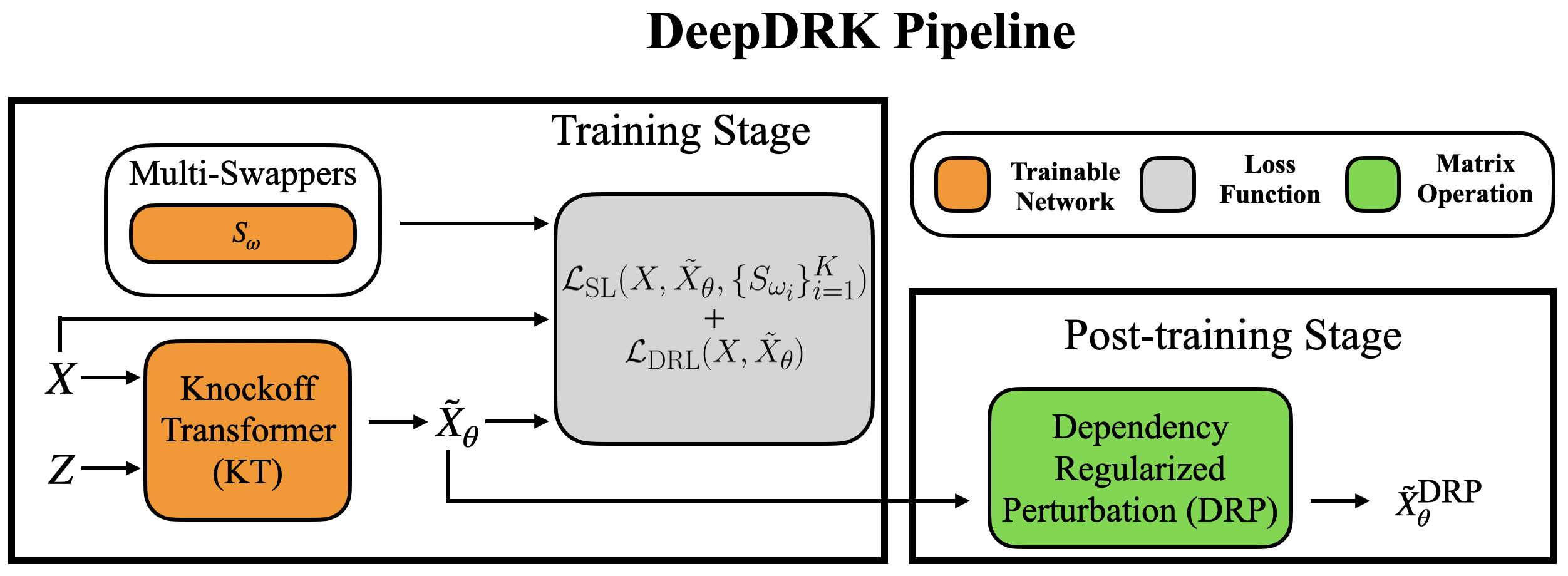
DeepDRK provides a novel way to generate knockoffs while reducing the reconstructability (see Section 2.3) between the generated knockoff and the input for data with complex distributions. Note that in this section we slightly abuse the notation such that and denote the corresponding data matrices. The generated knockoff can then be used to perform FDR-controlled feature selection following the Model-X knockoff framework (see Section 2.1). Overall, DeepDRK is a pipeline of two components. It first trains a transformer-based deep learning model, denoted as Knockoff Transformer (KT), to obtain swap property as well as reduce recontructability for the generated knockoff, with the help of adversarial attacks via multi-swappers. Second, a dependency regularized perturbation technique (DRP) is developed to further reduce the reconstructability for post training. In the following subsections, we discuss two components in detail in the following two subsections.
3.1 Training with Knockoff Transformer and Swappers
The KT (i.e. ), shown in Fig. 1, is trained to generate knockoffs by minimizing a swap loss (SL) and a dependency regularization loss (DRL) to achieve swap property and boost power. Swappers (i.e. ), on the other hand, are trained to generate adversarial swaps to enforce swap property. The total training objective is defined as
| (6) |
Note that we use and interchangeably, whereas the former is to emphasize that the knockoff depends on the model weights for KT. We detail the design of KT and swappers in Appendix C. In the following subsections, we breakdown each loss function.
3.1.1 Swap Loss
The swap loss is designed to enforce the swap property and is defined as follow:
| (7) |
where and are hyperparameters.
The first term in Eq. (3.1.1)—“SWD"—measures the distance between two corresponding distributions. In our case, they are the laws of the joint distributions and . Here is the sliced-Wasserstein distance (see Appendix D), is the -th swapper with model parameters , and is the total number of swappers. The swapper, introduced in [56], is a neural network for generating adversarial swaps (i.e. attacks). Training against such attacks enforces the swap property (see Appendix C for a detailed description). We adopt the same idea and extend it to a “multi-swapper" setup that jointly optimizes multiple independent swappers to better achieve swap property. In comparison with the likelihood-based loss in [56], which requires a normalizing flow (NF) [45] to fit, SWD is adopted to compare distributions, as it not only demonstrates high performance on complex structures such as multi-modal data, but also fast to implement since it is likelihood-free [28, 14, 15, 42].
The second term in Eq. (3.1.1)—“REx"—stands for risk extrapolation [30] and is defined here as for , which is a variant of the invariant risk minimization (IRM) [3] loss. This term is commonly used to add robustness against adversarial attacks in generative modeling, which in our case, guarantees that the generated knockoffs are robust to multiple swap attacks simultaneously. Since swappers may have the same effect (identical adversarial attacks) if they share the same weights , it is important to distinguish them by enforcing different pairs of weights via the third term in Eq. (3.1.1):
| (8) |
where , and is the cosine similarity function.
3.1.2 Dependency Regularization Loss
As discussed in Section 2.2, pursuing the swap property on sample level often leads to severe overfitting of (i.e., pushing towards ), which results in high collinearity in feature selection. To remedy, the DRL is introduced to reduce the reconstructability between and :
| (9) |
where is a hyperparameter. The SWC term in Eq. (9) refers to the sliced-Wasserstein correltaion [33], which quantitatively measures the dependency between two random vectors in the same space. More specifically, let and be two -dimensional random vectors. indicates that and are independent, while suggests a linear relationship between each other (see Appendix E for more details of SWC). In DeepDRK, we minimize SWC to reduce the reconstructability, a procedure similar to [55]. The intuition is as follows. If the joint distribution of is known, then for each , the knockoff should be independently sampled from . In such case the swap property is ensured, and collinearity is avoided due to independence. As we do not have access to the joint law, we want the variables to be less dependent. Since collinearity exists with in , merely decorrelate and is not enough. Thus we minimize SWC so that and are less dependent. We refer readers to Appendix B for further discussion.
3.2 Dependency Regularization Perturbation
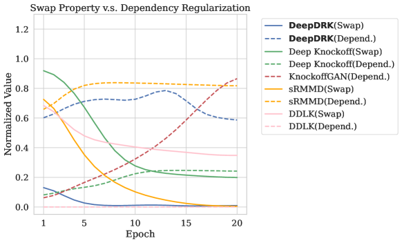
Empirically we observe a competition between and in Eq. (6), which adds difficulty to the training procedure. Specifically, the is dominating and the increases quickly after a short decreasing period. The phenomenon is also observed in all deep-learning based knockoff generation models when one tries to gain power [48, 56, 38, 27]. We inlcude the experimental evidence in Appendix F. We speculate the reasons as follows: minimizing the swap loss, which corresponds to FDR control, is the same as controlling Type I error. Similarly, minimizing the dependency loss is to control Type II error. With a fixed number of observations, it is well known that Type I error and Type II error can not decrease at the same time after reaching a certain threshold. In the framework of model-X knockoff, we aim to boost as much power as possible given the FDR is controlled at a certain level, a similar idea as the uniformly most powerful (UMP) test [13]. For this reason, we propose DRP as a post-training technique to further boost power.
DRP is a sample-level perturbation that further eliminates dependency between and and the knockoff. More specifically, DRP perturbs the generated with the row-permuted version of , denoted as . After applying DRP, the final knockoff becomes:
| (10) |
where is a preset perturbation weight. In this way has a smaller SWC with , since is independent of . Apparently by the perturbation, swap loss increases. We show in Appendix I and J.1 the effect of the perturbation on the swap property, FDR, and power.
4 Experiment
We compare the performance of our proposed DeepDRK with a set of benchmarking models from three different perspectives. Namely, we focus on: 1. the fully synthetic setup that both input variables and the response variable have pre-defined distributions; 2. the semi-synthetic setup where input variables are rooted in real-world datasets and the response variable is created according to some known relationships with the input; 3. FS with a real-world dataset. Overall, the experiments are designed to cover various datasets with different ratios and different distributions of , aiming to evaluate the model performance comprehensively. In the following, we first introduce the model and training setups for DeepDRK and the benchmarking models. Next we discuss the configuration of the feature selection. Finally, we describe the dataset setups, and the associated results are presented. Additionally, we consider the ablation study to illustrate the benefits obtained by having the following proposed terms: REx, , the multi-swapper setup, and the dependency regularization perturbation. Empirically, these terms improve power and enforce the swap property for a lower FDR. Due to space limitation, we defer details to Appendix J.2 and J.3.
4.1 Model Training & Configuration
To fit models, we first split datasets of into two parts, with an 8:2 training and validation ratios. The training sets are then used for model optimization, and validation sets are used for stopping the model training with an early stop rule on the validation loss with the patient period equals 6. Since knockoffs are not unique [12], there is no need of the testing sets. To evaluate the model performance of DeepDRK, we compare it with 4 state-of-the-art (SOTA) deep-learning-based knockoff generation models as we focus on non-parametric data in this paper. Namely, we consider Deep Knockoff [48] 222https://github.com/msesia/deepknockoffs, DDLK [56] 333https://github.com/rajesh-lab/ddlk, KnockoffGAN [27] 444https://github.com/vanderschaarlab/mlforhealthlabpub/tree/main/alg/knockoffgan and sRMMD [38] 555https://github.com/ShoaibBinMasud/soft-rank-energy-and-applications, with links of the code implementation listed in the footnote. We follow all the recommended hyperparameter settings for training and evaluation in their associated code repositories. The only difference is the total number of training epochs. To maintain consistency, we set this number to 200 for all models (including DeepDRK).
We follow the model configuration (see Appendix G) to optimize DeepDRK. The architecture of the swappers is adopted from [56]. Optimizers for training both swappers and are AdamW [36]. We interchangeably optimize for and swappers during training (see Eq. (6)). For every three times of updates for weights , the weights are updated once. The training scheme is similar to the training of GAN [21], except the absence of discriminators. We also apply early stopping criteria to prevent overfitting. A pseudo code for the optimization can be found in Appendix H. To conduct experiments, we set universally for the dependency regularization coefficient as it leads to consistent performance across all experiments. A discussion on the effect of is detailed in Appendix I.
Once models are trained, we generate the knockoff given the data of . The generated are then combined with for feature selection. We run each experiment on a single NVIDIA V100 16GB GPU. DeepDRK is implemented by PyTorch [46] 666The implementation of DeepDRK can be found in https://github.com/nowonder2000/DeepDRK..
4.2 Feature Selection Configuration
Once the knockoff is obtained, feature selection is performed following three steps. First, concatenate to form a design matrix . Second, fit a regression model to obtain estimation coefficients . We use Ridge regression as it generally results in higher power. Third, compute knockoff statistics (for ), and select features according to Eq. (5). We consider as the FDR threshold due to its wide application in the analysis by other knockoff-based feature selection papers [48, 38]. Each experiment is repeat 600 times, and the following results with synthetic and semi-synthetic datasets are provided with the average power and FDR of the 600 repeats.
4.3 The Synthetic Experiments
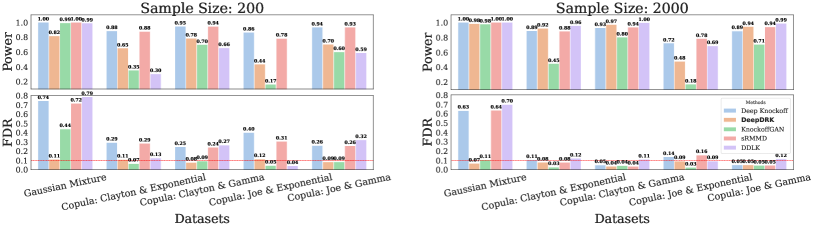
To properly evaluate the performance, we follow a well-designed experimental setup by [56, 38] to generate different sets of -samples of . Here is the collection dependent variables that follows pre-defined distributions. is the response variable that is modeled as . The underlying true is the -dimensional coefficient which is set to follow . Compared to [56] and [38], which consider as the scalar for the Rademacher, we downscale the scale of by the factors of 15. This is because we find that in the original setup, the scale is too large such that the feature selection enjoys high powers and low FDRs for all models. To compare the performance of the knockoff generation methods on various data, we consider the following distributions for :
Mixture of Gaussians: Following [56], we consider a Gaussian mixture model , where is the proportion of the -th Gaussian with . denotes the mean of the -th Gaussian with , where is the -dimensional vector that has universal value 1 for all entries. is the covariance matrices whose -th entry taking the value , where and . Besides this experiment, we further test with Mixture of Gaussian data of various to study the feature selection performance with highly correlated features. Namely, we consider additional .
Copulas [50]: we further use copula to model complex correlations within . To our knowledge, this is a first attempt to consider complicated distributions other than the mixture Gaussian in the knockoff framework. Specifically, we consider two copula families: Clayton, Joe with the consistent copula parameter of 2 in both cases. For each family, two candidates of the marginal distributions are considered: uniform (i.e. identity conversion function) and the exponential distribution with rate equals 1. We implement copulas according to PyCop 777https://github.com/maximenc/pycop/.
We consider the following setups in the form of tuples: (200, 100) and (2000, 100). This is in contrast to existing works, which considers only the (2000, 100) case for small value [56, 38, 48]. Our goal is to demonstrate a consistent performance by the proposed DeepDRK on different ratios, especially when it is small.
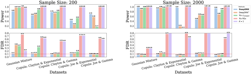
Results: Figure 2 compare FDRs and Powers for all models across the previously introduced datasets with two different setups for , respectively. It is observed in Figure 2 that DeepDRK is capable of controlling FDR consistently compared to other benchmarking models across different data distributions and different ratios except for a few FDR-inflated cases (i.e. above the 0.1 threshold) in the low sample size setup. Other models, though being able to reach higher power, comes at a cost of sacrificing FDR, which contradicts to the UMP philosophy (see Section 3.2). Additionally, we consider a comparison between the Mixture of Gaussian data with growing values of , which indicates the increased correlation between the input variables. Note that the Gaussian mixture in Figure 2 has . The results for are presented in Figure 3. Compared to other benchmarking models, DeepDRK maintain the lowerest FDRs while generating competitive powers on all setups suggesting its capacity to fight against correlation in data . Overall, the results demonstrate the ability of DeepDRK in consistently performing FS with controlled FDR compared to other models across a range of different datasets, ratios, and feature correlations in .
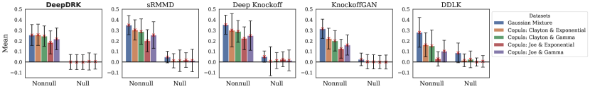
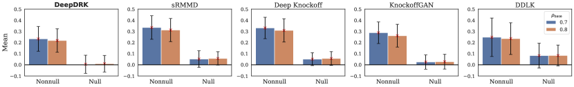
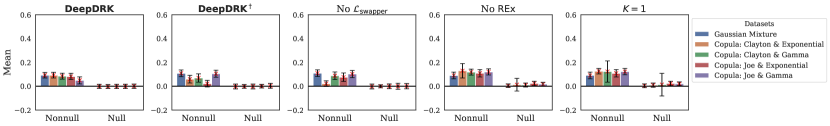
To properly justify why DeepDRK outperforms other benchmarking models, we consider measuring the distribution of the knockoff statistics (i.e. ) for both nonnull and null features of . Both fan2023ark [17] and candes2018panning [12] point out that a good knockoff requires the corresponding knockoff statistics to concentrate symmetrically around zero for the null features and to maintain high positive values for the nonnulls. However, theoretical analysis on the goodness of FDR or power requires access to the true knockoff [17], to compare the distribution of ’s with the ground truth, which is infeasible for complex distributions in practice. Nevertheless, we can still investigate the distribution of the knockoff statistics as a surrogate to analyze the performance of models in FDR or power given the aforementioned properties required by the knockoff statistics [17, 12].
We present the empirical measurement of the distribution for the knockoff statistics ’s in Figure 4. The figure includes the distribution (e.g. both mean and standard deviation) for both null and nonnull variables across different dataets and models. Clearly, compared to other benchmarks, DeepDRK maintains high ’s for the nonnulls and relatively symmetric values around zero for the nulls. All other models experience positive shifts to the null statistics to some extent. The reason positive shifts lead to a degeneracy in performance is that the rule of choosing the threshold for FS is based on the negative values of ’s (see Eq. (5)). A positive shift for the null statistics has two negative impacts on the threshold and its subsequent FS process. First, the shift makes the threshold to be close to zero as fewer null statistics remain on the negative side. Second, after a sign flip, this threshold is used for selecting features in the knockoff framework. However, since the sign flip maintains the distance between the threshold and zero, a positive shift of the null statistics indicates more values of the null statistics will exceed this close-to-zero threshold, resulting more false positives. By Figure 2, since DeepDRK achieves good FDR controllability and high power, it is expectedly to believe its knockoff statistics are around zero for the nulls, in contrast to the nonnulls that have large positive values. And this is empirically verified in Figure 4. Due to space limit, we defer the sample-size-2000 case and the comparison of ’s for the Gaussian correlation setup (i.e. Figure 3) in Appendix J.3.
4.4 The Semi-synthetic Experiments
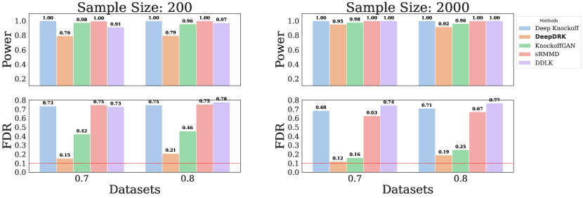
Following [23] and [56], we consider a semi-synthetic study with design drawn from two real-world datasets, and use to simulate response . The details of which are as follows:
The first dataset contains single-cell RNA sequencing (scRNA-seq) data from 10x Genomics 888https://kb.10xgenomics.com/hc/en-us. Each entry in represents the observed gene expression of gene in cell . We refer readers to [23] and [1] for further background. Following the same preprocessing in [23], we obtain the final dataset of is of size 10000 and dimension 100 999The data processing code is adopted from this repo: https://github.com/dereklhansen/flowselect/tree/master/data. The preprocessing of and the synthesis of are deferred in Appendix L.
The second publicly available101010https://www.metabolomicsworkbench.org/ under the project DOI: 10.21228/M82T15. dataset originates from a real case study entitled “Longitudinal Metabolomics of the Human Microbiome in Inflammatory Bowel Disease (IBD)” [35]. The study seeks to identify important metabolites of two representative diseases of the inflammatory bowel disease (IBD): ulcerative colitis (UC) and Crohn’s disease (CD). Specifically, we use the C18 Reverse-Phase Negative Mode dataset that has 546 samples, each of which has 91 metabolites (i.e. ). To mitigate the effects of missing values, we preprocess the dataset following a common procedure to remove metabolites that have over 20% missing values, resulting in 80 metabolites, which are then normalized to have zero mean and unit variance after a log transform and an imputation via the k nearest neighbor algorithm following the same procedure in [38]. Finally, we synthesize the response with the real dataset of via , where follows entry-wise Unif(0, 1), , and Rademacher(0.5) distributions.
Model DeepDRK Deep Knockoff sRMMD KnockoffGAN DDLK Referenced / Identified 19/23 15/20 5/5 12/14 17/25
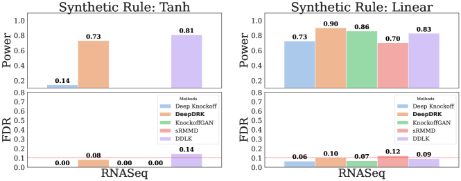
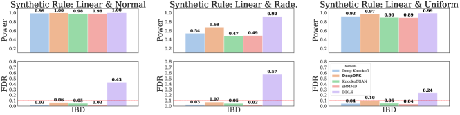
Results: Figure 5 and 6 compare the feature selection performance on the RNA data and the IBD data respectively. In Figure 5, we observe that all but DDLK are bounded by the nominal 0.1 FDR threshold in the “Tanh" case. However, KnockoffGAN and sRMMD have almost zero power. The power for Deep Knockoff is also very low compared to that of DeepDRK. Although DDLK provides high power, the associated FDR is undesirable. In the “Linear" case, almost all models have well controlled FDR, among which DeepDRK provides the highest power. Similar observations can be found in Figure 6. For the IBD data under the aforementioned three different data synthesis rules, it is clear all models but DDLK achieve well-controlled FDR. Apart from DDLK, DeepDRK universally achieves the highest powers. The results further demonstrate the potential of DeepDRK on real data applications.
4.5 A Case Study
Besides (semi-)synthetic setups, we follow [56, 48] and carry out a case study with real data for both design and response , in order to qualitatively evaluate the selection performance of DeepDRK. In this subsection, we consider the full IBD dataset (i.e. with both and from the dataset [35]). The response variable is categorical: equals 1 if a given sample is associated with UC/CD and 0 otherwise. The covariates is identical to the second semi-synthetic setup considered in Section 4.4. To properly evaluate results with no ground truth available, we investigate literature with different sources, searching for the evidence of the IBD-associated metabolites. Namely, we curate three sources: 1. metabolites that are explicitly documented to have associations with IBD, UC, or CD in the PubChem database 111111https://pubchem.ncbi.nlm.nih.gov/; 2. metabolites that are reported in the existing peer-reviewed publications; 3. metabolites that are reported in pre-prints. To our knowledge, we are the first to carry out a comprehensive metabolite investigation for the IBD dataset. All referenced metabolites are included in Table 6 in Appendix M. In all, we identify 47 metabolites that are reported to have association with IBD.
To evaluate model performance, we first consider the same setup (see Table 2 in Appendix G) to train the model and generate knockoffs using the DeepDRK pipeline. During the FS step, however, we use 0.2 as the FDR threshold instead of 0.1, and apply a different algorithm—DeepPINK [37] that is included in the knockpy 121212https://amspector100.github.io/knockpy/ library—to generate knockoff statistics . The values are subsequently used to identify metabolites. We choose DeepPINK—a neural-network-based model–over the previously considered ridge regression due to the nonlinear relationships between metabolites (i.e. ) and labels (i.e. ) in this case study. Likewise, to generate knockoff for the benchmarking models, we follow their default setup. During FS, same changes are applied as in DeepDRK.
We compare the FS results with the 47 metabolites and report the number of selections in Table 1. A detailed list of selected features for each model can be found in Table 7 in Appendix M. From Table 1, we clearly observe that compared to the benchmarking models, DeepDRK identifies the most number of referenced metabolites while limiting the discovered metabolites that are not yet documented in the literature (see Table 6 in Appendix M). KnockoffGAN and sRMMD behave preferably in limiting the number of discoveries given the fewer number of identified undocumented metabolites. The performance of Deep Knockoff and DDLK is intermediate, meaning a relatively higher number of discovered metabolites that are referenced, compared to KnockoffGAN and sRMMD, and a relatively lower number of discovered undocumented metabolites. Nevertheless, since there is no ground truth available, the comparison is only qualitative.
5 Conclusion
In this paper, we first discover a competing relationship between the “swap property" and the feature selection power on sample levels. This, to our knowledge, has never been reported before. As a remedy, we introduce DeepDRK, a deep learning-based knockoff generation pipeline that consists of two steps. It first trains a Knockoff Transformer with multi-swappers to obtain swap property as well as reduce reconstructability. Second, the dependency regularized perturbation is applied to further boost power after training. DeepDRK is shown to achieve both low FDR and high power across various data distributions, with different ratios. Additionally, we provide interpretation on the distribution of knockoff statistics that further reveals the reason of DeepDRK’s consistent performance. Overall, results suggest an outperformance of DeepDRK over all considered deep-learning-based benchmarking models. Experiments with real and semi-synthetic data further demonstrate the potential of DeepDRK in feature selection tasks with complex data structures.
References
- [1] Divyansh Agarwal, Jingshu Wang, and Nancy R Zhang. Data denoising and post-denoising corrections in single cell rna sequencing. 2020.
- [2] Ashwin N Ananthakrishnan, Chengwei Luo, Vijay Yajnik, Hamed Khalili, John J Garber, Betsy W Stevens, Thomas Cleland, and Ramnik J Xavier. Gut microbiome function predicts response to anti-integrin biologic therapy in inflammatory bowel diseases. Cell host & microbe, 21(5):603–610, 2017.
- [3] Martin Arjovsky, Léon Bottou, Ishaan Gulrajani, and David Lopez-Paz. Invariant risk minimization. arXiv preprint arXiv:1907.02893, 2019.
- [4] Martin Arjovsky, Soumith Chintala, and Léon Bottou. Wasserstein generative adversarial networks. In International conference on machine learning, pages 214–223. PMLR, 2017.
- [5] Rina Foygel Barber and Emmanuel J Candès. Controlling the false discovery rate via knockoffs. 2015.
- [6] Cristina Bauset, Laura Gisbert-Ferrándiz, and Jesús Cosín-Roger. Metabolomics as a promising resource identifying potential biomarkers for inflammatory bowel disease. Journal of Clinical Medicine, 10(4):622, 2021.
- [7] Yoav Benjamini and Yosef Hochberg. Controlling the false discovery rate: a practical and powerful approach to multiple testing. Journal of the Royal statistical society: series B (Methodological), 57(1):289–300, 1995.
- [8] Shoaib Bin Masud, Conor Jenkins, Erika Hussey, Seth Elkin-Frankston, Phillip Mach, Elizabeth Dhummakupt, and Shuchin Aeron. Utilizing machine learning with knockoff filtering to extract significant metabolites in crohn’s disease with a publicly available untargeted metabolomics dataset. Plos one, 16(7):e0255240, 2021.
- [9] PA Blaker, M Arenas-Hernandez, MA Smith, EA Shobowale-Bakre, L Fairbanks, PM Irving, JD Sanderson, and AM Marinaki. Mechanism of allopurinol induced tpmt inhibition. Biochemical pharmacology, 86(4):539–547, 2013.
- [10] Nicolas Bonneel, Julien Rabin, Gabriel Peyré, and Hanspeter Pfister. Sliced and radon wasserstein barycenters of measures. Journal of Mathematical Imaging and Vision, 51:22–45, 2015.
- [11] Nicolas Bonnotte. Unidimensional and evolution methods for optimal transportation. PhD thesis, Université Paris Sud-Paris XI; Scuola normale superiore (Pise, Italie), 2013.
- [12] Emmanuel Candes, Yingying Fan, Lucas Janson, and Jinchi Lv. Panning for gold:‘model-x’knockoffs for high dimensional controlled variable selection. Journal of the Royal Statistical Society: Series B (Statistical Methodology), 80(3):551–577, 2018.
- [13] George Casella and Roger L Berger. Statistical inference. Cengage Learning, 2021.
- [14] Ishan Deshpande, Yuan-Ting Hu, Ruoyu Sun, Ayis Pyrros, Nasir Siddiqui, Sanmi Koyejo, Zhizhen Zhao, David Forsyth, and Alexander G Schwing. Max-sliced wasserstein distance and its use for gans. In Proceedings of the IEEE/CVF Conference on Computer Vision and Pattern Recognition, pages 10648–10656, 2019.
- [15] Ishan Deshpande, Ziyu Zhang, and Alexander G Schwing. Generative modeling using the sliced wasserstein distance. In Proceedings of the IEEE conference on computer vision and pattern recognition, pages 3483–3491, 2018.
- [16] Alexey Dosovitskiy, Lucas Beyer, Alexander Kolesnikov, Dirk Weissenborn, Xiaohua Zhai, Thomas Unterthiner, Mostafa Dehghani, Matthias Minderer, Georg Heigold, Sylvain Gelly, et al. An image is worth 16x16 words: Transformers for image recognition at scale. arXiv preprint arXiv:2010.11929, 2020.
- [17] Yingying Fan, Lan Gao, and Jinchi Lv. Ark: Robust knockoffs inference with coupling. arXiv preprint arXiv:2307.04400, 2023.
- [18] DJ Fretland, DL Widomski, S Levin, and TS Gaginella. Colonic inflammation in the rabbit induced by phorbol-12-myristate-13-acetate. Inflammation, 14(2):143–150, 1990.
- [19] Yulia Gavrilov, Yoav Benjamini, and Sanat K Sarkar. An adaptive step-down procedure with proven fdr control under independence. The Annals of Statistics, 37(2):619–629, 2009.
- [20] Jaime Roquero Gimenez, Amirata Ghorbani, and James Zou. Knockoffs for the mass: new feature importance statistics with false discovery guarantees. In The 22nd international conference on artificial intelligence and statistics, pages 2125–2133. PMLR, 2019.
- [21] Ian Goodfellow, Jean Pouget-Abadie, Mehdi Mirza, Bing Xu, David Warde-Farley, Sherjil Ozair, Aaron Courville, and Yoshua Bengio. Generative adversarial networks. Communications of the ACM, 63(11):139–144, 2020.
- [22] Isabelle Guyon and André Elisseeff. An introduction to variable and feature selection. Journal of machine learning research, 3(Mar):1157–1182, 2003.
- [23] Derek Hansen, Brian Manzo, and Jeffrey Regier. Normalizing flows for knockoff-free controlled feature selection. Advances in Neural Information Processing Systems, 35:16125–16137, 2022.
- [24] Zihuai He, Linxi Liu, Chen Wang, Yann Le Guen, Justin Lee, Stephanie Gogarten, Fred Lu, Stephen Montgomery, Hua Tang, Edwin K Silverman, et al. Identification of putative causal loci in whole-genome sequencing data via knockoff statistics. Nature communications, 12(1):1–18, 2021.
- [25] Marian Hristache, Anatoli Juditsky, and Vladimir Spokoiny. Direct estimation of the index coefficient in a single-index model. Annals of Statistics, pages 595–623, 2001.
- [26] Eric Jang, Shixiang Gu, and Ben Poole. Categorical reparameterization with gumbel-softmax. In 5th International Conference on Learning Representations, ICLR 2017, Toulon, France, April 24-26, 2017, Conference Track Proceedings. OpenReview.net, 2017.
- [27] James Jordon, Jinsung Yoon, and Mihaela van der Schaar. Knockoffgan: Generating knockoffs for feature selection using generative adversarial networks. In International Conference on Learning Representations, 2018.
- [28] Soheil Kolouri, Kimia Nadjahi, Umut Simsekli, Roland Badeau, and Gustavo Rohde. Generalized sliced wasserstein distances. Advances in neural information processing systems, 32, 2019.
- [29] Hon Wai Koon. A novel orally active metabolite reverses crohn’s disease-associated intestinal fibrosis. Inflammatory Bowel Diseases, 28(Supplement_1):S61–S62, 2022.
- [30] David Krueger, Ethan Caballero, Joern-Henrik Jacobsen, Amy Zhang, Jonathan Binas, Dinghuai Zhang, Remi Le Priol, and Aaron Courville. Out-of-distribution generalization via risk extrapolation (rex). In International Conference on Machine Learning, pages 5815–5826. PMLR, 2021.
- [31] Aonghus Lavelle and Harry Sokol. Gut microbiota-derived metabolites as key actors in inflammatory bowel disease. Nature reviews Gastroenterology & hepatology, 17(4):223–237, 2020.
- [32] Thomas Lee, Thomas Clavel, Kirill Smirnov, Annemarie Schmidt, Ilias Lagkouvardos, Alesia Walker, Marianna Lucio, Bernhard Michalke, Philippe Schmitt-Kopplin, Richard Fedorak, et al. Oral versus intravenous iron replacement therapy distinctly alters the gut microbiota and metabolome in patients with ibd. Gut, 66(5):863–871, 2017.
- [33] Tao Li, Jun Yu, and Cheng Meng. Scalable model-free feature screening via sliced-wasserstein dependency. Journal of Computational and Graphical Statistics, pages 1–11, 2023.
- [34] Ying Liu and Cheng Zheng. Auto-encoding knockoff generator for fdr controlled variable selection. arXiv preprint arXiv:1809.10765, 2018.
- [35] Jason Lloyd-Price, Cesar Arze, Ashwin N Ananthakrishnan, Melanie Schirmer, Julian Avila-Pacheco, Tiffany W Poon, Elizabeth Andrews, Nadim J Ajami, Kevin S Bonham, Colin J Brislawn, et al. Multi-omics of the gut microbial ecosystem in inflammatory bowel diseases. Nature, 569(7758):655–662, 2019.
- [36] Ilya Loshchilov and Frank Hutter. Decoupled weight decay regularization. arXiv preprint arXiv:1711.05101, 2017.
- [37] Yang Lu, Yingying Fan, Jinchi Lv, and William Stafford Noble. Deeppink: reproducible feature selection in deep neural networks. Advances in neural information processing systems, 31, 2018.
- [38] Shoaib Bin Masud, Matthew Werenski, James M Murphy, and Shuchin Aeron. Multivariate rank via entropic optimal transport: sample efficiency and generative modeling. arXiv preprint arXiv:2111.00043, 2021.
- [39] Rishi S Mehta, Zachary L Taylor, Lisa J Martin, Michael J Rosen, and Laura B Ramsey. Slco1b1* 15 allele is associated with methotrexate-induced nausea in pediatric patients with inflammatory bowel disease. Clinical and translational science, 15(1):63–69, 2022.
- [40] Itta M Minderhoud, Bas Oldenburg, Marguerite EI Schipper, Jose JM Ter Linde, and Melvin Samsom. Serotonin synthesis and uptake in symptomatic patients with crohn’s disease in remission. Clinical Gastroenterology and Hepatology, 5(6):714–720, 2007.
- [41] Rajagopalan Lakshmi Narasimhan, Allison A Throm, Jesvin Joy Koshy, Keith Metelo Raul Saldanha, Harikrishnan Chandranpillai, Rahul Deva Lal, Mausam Kumravat, Ajaya Kumar KM, Aneesh Batra, Fei Zhong, et al. Inferring intestinal mucosal immune cell associated microbiome species and microbiota-derived metabolites in inflammatory bowel disease. bioRxiv, 2020.
- [42] Khai Nguyen, Tongzheng Ren, Huy Nguyen, Litu Rout, Tan Nguyen, and Nhat Ho. Hierarchical sliced wasserstein distance. arXiv preprint arXiv:2209.13570, 2022.
- [43] Thomas Giacomo Nies, Thomas Staudt, and Axel Munk. Transport dependency: Optimal transport based dependency measures. arXiv preprint arXiv:2105.02073, 2021.
- [44] Andrea Nuzzo, Somdutta Saha, Ellen Berg, Channa Jayawickreme, Joel Tocker, and James R Brown. Expanding the drug discovery space with predicted metabolite–target interactions. Communications biology, 4(1):1–11, 2021.
- [45] George Papamakarios, Eric Nalisnick, Danilo Jimenez Rezende, Shakir Mohamed, and Balaji Lakshminarayanan. Normalizing flows for probabilistic modeling and inference. The Journal of Machine Learning Research, 22(1):2617–2680, 2021.
- [46] Adam Paszke, Sam Gross, Francisco Massa, Adam Lerer, James Bradbury, Gregory Chanan, Trevor Killeen, Zeming Lin, Natalia Gimelshein, Luca Antiga, et al. Pytorch: An imperative style, high-performance deep learning library. Advances in neural information processing systems, 32, 2019.
- [47] Xiaofa Qin. Etiology of inflammatory bowel disease: a unified hypothesis. World journal of gastroenterology: WJG, 18(15):1708, 2012.
- [48] Yaniv Romano, Matteo Sesia, and Emmanuel Candès. Deep knockoffs. Journal of the American Statistical Association, 115(532):1861–1872, 2020.
- [49] Sameh Saber, Rania M Khalil, Walied S Abdo, Doaa Nassif, and Eman El-Ahwany. Olmesartan ameliorates chemically-induced ulcerative colitis in rats via modulating nfb and nrf-2/ho-1 signaling crosstalk. Toxicology and applied pharmacology, 364:120–132, 2019.
- [50] Thorsten Schmidt. Coping with copulas. Copulas-From theory to application in finance, 3:1–34, 2007.
- [51] Elizabeth A Scoville, Margaret M Allaman, Caroline T Brown, Amy K Motley, Sara N Horst, Christopher S Williams, Tatsuki Koyama, Zhiguo Zhao, Dawn W Adams, Dawn B Beaulieu, et al. Alterations in lipid, amino acid, and energy metabolism distinguish crohn’s disease from ulcerative colitis and control subjects by serum metabolomic profiling. Metabolomics, 14(1):1–12, 2018.
- [52] Matteo Sesia, Chiara Sabatti, and Emmanuel J Candès. Gene hunting with knockoffs for hidden markov models. arXiv preprint arXiv:1706.04677, 2017.
- [53] Johan D Söderholm, Gunnar Olaison, KH Peterson, LE Franzen, T Lindmark, Mikael Wirén, Christer Tagesson, and Rune Sjödahl. Augmented increase in tight junction permeability by luminal stimuli in the non-inflamed ileum of crohn’s disease. Gut, 50(3):307–313, 2002.
- [54] Johan D Soderholm, Hans Oman, Lars Blomquist, Joggem Veen, Tuulikki Lindmark, and Gunnar Olaison. Reversible increase in tight junction permeability to macromolecules in rat ileal mucosa in vitro by sodium caprate, a constituent of milk fat. Digestive diseases and sciences, 43(7):1547–1552, 1998.
- [55] Asher Spector and Lucas Janson. Powerful knockoffs via minimizing reconstructability. The Annals of Statistics, 50(1):252–276, 2022.
- [56] Mukund Sudarshan, Wesley Tansey, and Rajesh Ranganath. Deep direct likelihood knockoffs. Advances in neural information processing systems, 33:5036–5046, 2020.
- [57] Karsten Suhre, So-Youn Shin, Ann-Kristin Petersen, Robert P Mohney, David Meredith, Brigitte Wägele, Elisabeth Altmaier, Panos Deloukas, Jeanette Erdmann, Elin Grundberg, et al. Human metabolic individuality in biomedical and pharmaceutical research. Nature, 477(7362):54–60, 2011.
- [58] Kan Uchiyama, Shunichi Odahara, Makoto Nakamura, Shigeo Koido, Kiyohiko Katahira, Hiromi Shiraishi, Toshifumi Ohkusa, Kiyotaka Fujise, and Hisao Tajiri. The fatty acid profile of the erythrocyte membrane in initial-onset inflammatory bowel disease patients. Digestive diseases and sciences, 58(5):1235–1243, 2013.
- [59] Victor Uko, Suraj Thangada, and Kadakkal Radhakrishnan. Liver disorders in inflammatory bowel disease. Gastroenterology research and practice, 2012, 2012.
- [60] Ashish Vaswani, Noam Shazeer, Niki Parmar, Jakob Uszkoreit, Llion Jones, Aidan N Gomez, Łukasz Kaiser, and Illia Polosukhin. Attention is all you need. Advances in neural information processing systems, 30, 2017.
- [61] Cédric Villani et al. Optimal transport: old and new, volume 338. Springer, 2009.
- [62] Johannes CW Wiesel. Measuring association with wasserstein distances. Bernoulli, 28(4):2816–2832, 2022.
Appendix
Appendix A FDR definition
The definition of FDR is a follows. Let be any selected indices and be the underlying true regression coefficients. The FDR for selection is
| (11) |
Appendix B Reconstructability and Selection Power
The notion of reconstructability is introduced by [55] as a population level counterpart of what is usually referred to as collinearity in linear regression. Under Gaussian design where , reconstructability is high if is not of fill rank, so that s.t. is a.s. a linear combination of . More generally, if there exists more than one representation of the response using the explanatory variable , we qualitatively say that the recontructability is high. As high collinearity often causes trouble, reconstructability also hurts power in feature selection. To better illustrate, we state a linear version of Theorem 2.3 in [55], which is originally a more general single-index model [25].
Theorem 2.
Let , where , and is a centered Gaussian noise. Equivalently it means . Suppose there exists a such that a.s., then denoting , we have
| (12) |
Furthermore in the knockoff framework [5], let and , then for all ,
| (13) |
Equation 13 implies a no free lunch situation for selection power when there is exact reconstructability.
To fix the recontructability issue, [55] proposed two methods in Guassian design. The first is the minimal variance-based reconstructability (MVR) knockoff, in which knockoff is sampled to minimize the loss
| (14) |
Note that is equivalent to maximize for all . Another way to achieve it is the maximum entropy (ME) knockoff, where is sampled from maximizing
| (15) |
Fortunately under Gaussian design, the above two optimizations have closed-form solutions. Since is Guassian, must be joint Gaussian to satisfy the swap property. To optimize, one first calculates the covariance matrix using the SDP method in [5], which gives a diagonal matrix . Then both MVR and ME boils down to an optimization on :
| (16) |
Though it is shown that both methods obtain high power for feature selection, however, neither MVR nor ME could be directly extended to arbitrary distributions, due to the fact that the conditional variance and the likelihood is intractable.
In DeepDRK, we consider regularizing with a sliced-Wasserstein-based dependency correlation, which can be deemed a stronger dependency regularization than entropy. A post-training perturbation is also applied to further reduce collinearity. However, theoretical understanding of how they affect swap property and power remains to be studied.
Appendix C The Design of Knockoff Transformer and Swappers
DeepDRK’s knockoff Transformer (KT) model is designed based on the popular Vision Transformer (ViT) [16]. The difference being the dimension of the input is 1D, not 2D, for . We do not consider patches as the input. Instead, we consider all entries of to consider correlations of each pair of entries in the knockoff . This is structurally similar to the original Transformer [60]. Nonetheless, we keep all the remaining components from ViT, such as patch embedding, PreNorm and 1D-positional encoding [16]. Since knockoff generation essentially requires a distribution. To enable this, we consider feeding and a uniformly distributed random variable of the same dimension as , to encode randomness.
The swapper module is first introduced in DDLK [56], to produce the index subset for the adversarial swap attack. Optimizing knockoff against these adversarial swaps enforces the swap property. Specifically, the swapper consists of a matrix of shape (i.e. trainable model weights), where is the dimension of . This matrix controls the Gumbel-softmax distribution [26] for all entries. Each entry is characterized by a binary Gumbel-softmax random variable (e.g. can only take values of 0 or 1). To generate the subset , we consider drawing samples of from the corresponding -th Gumbel-softmax random variable, and the subset is defined as . During optimization, we maximize Eq. (6) w.r.t. to the weights of the swapper such that the sampled indices, with which the swap is applied, lead to a higher SWD in the objective (Eq. (6)). Minimizing this objective w.r.t. requires the knockoff to fight against the adversarial swaps. Therefore, the swap property is enforced. Compared to DDLK, the proposed DeepDRK utilizes multiple independent swappers.
Appendix D From Wasserstein to Sliced-Wasserstein Distance
Wasserstein distance has become popular in both mathematics and machine learning due to its ability to compare different kinds of distributions [61] and almost everywhere differentiability [4]. Here we provide its definition. Let be two random vectors following distributions with finite -th moment. The Wasserstein- distance between and is:
| (17) |
where denotes the set of all joint distributions such that their marginals are and . When in particular, the Wasserstein distance between two one-dimensional distributions can be written as:
| (18) | ||||
where and are the cumulative distribution functions (CDF) of and respectively. Moreover, if as well, the Wasserstein distance can be further simplified as
| (19) |
From the above it is easy to notice that the Wasserstein distance is easy to compute, which leads to the development of sliced-Wasserstein distance (SWD) [10]. To exploit the computational advantage on , one first projects both distributions uniformly on a direction and computes the Wasserstein- distance between the two projected distributions. SWD is then calculated by taking the expectation of the random direction. More specifically, let denote a projection directions, the following push-forward distribution [61] denotes the law of . Let be dimensional spherical uniform, the -sliced-Wasserstein distance between and reads:
| (20) |
| (21) |
In spite of faster computations, the convergence of SWD is shown to be equivalent to the convergence of Wasserstein distance under mild condtions [11]. In practice, the expectation on is approximated by a finite summation over a number of projection directions uniformly chosen from .
Parameter Value Parameter Value # of 2 Temperature 0.2 Learning Rate Learning Rate Dropout Rate 0.1 # of Epochs 200 Batch Size 64 30.0 1.0 20.0 Early Stop Tolerance 6 # of Layers 8 # of heads in 8 Hidden Dim 512 0.5
Appendix E Sliced-Wasserstein Correlation
The idea of metricizing independence is recently advanced using the Wasserstein distance [62, 43]. Given a joint distribution and its marginal distributions , the Wasserstein Dependency (WD) between and is defined by . A trivial observation is that implies that and are independent. Due to the high computational cost of Wasserstein distance, sliced-Wasserstein dependency (SWDep) [33] is developed using sliced-Wasserstein distance (see Appendix D for SWD details). The SW dependency between and is defined as , and a SW dependency still indicates independence. Since the dependency metric is not bounded from above, sliced-Wasserstein correlation (SWC) is introduced to normalize SW dependency. More specifically, the SWC between and is defined as
| (22) |
where and are the joint distributions of and respectively. It is shown that and when has a linear relationship with [33].
In terms of computing SWC, we follow [33] and consider both laws of and to be sums of Diracs, i.e. both variables are empirical distributions with data . Define and , where . Because data is i.i.d., and are independent. We further introduce the following notation:
Then the empirical SWC can be computed by:
| (23) |
Appendix F Competing losses
In Figure 7, we include scaled curves and curves for each considered model. For comparison purposes, the curves that describe the changes of the corresponding losses are shown after normalizing the values to be within 0 and 1. We consider the first 20 epochs as the DRL would flatten out in latter epochs without dropping. The competition can be clearly observed as when drops, increases, indicating difficulty to maintain low reconstructability.
Appendix G Model Training Configuration
In Table 2, we include configuration details on the KT and swappers.
Appendix H Training Algorithm
Appendix I Effect of in
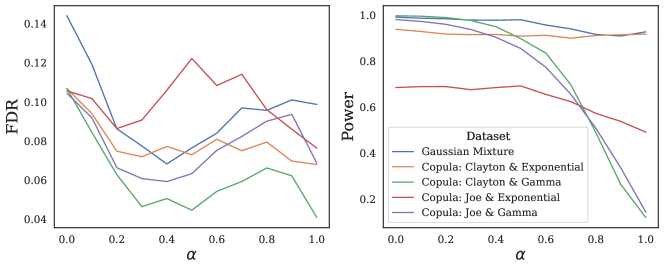
As discussed in section 3.2, empirically it is difficult to obtain swap property while maintaining low reconstructability at sample level. To leverage this issue, dependency regularization perturbation (DRP) is introduced. In this section, we evaluate the effect of in (e.g. Eq. (10)) to the feature selection performance. Results are summarized in Figure 8, concerning 5 synthetic datasets. When is decreased, we observe an increment in power. However, the FDR follows a bowel-shaped pattern. This is consistent with the statement in spector2022powerful [55], as introducing the permuted will decrease reconstructability for higher power. However, a dominating breaks the swap property for higher FDRs. Based on our hyperparameter search and the results in Figure 8, we suggest choosing within the range between 0.4 and 0.5.
Dataset MMD(Linear) SWD1 SWD2 DDLK J+G 2.68 0.18 0.08 C+G 2.49 0.18 0.07 C+E 1.80 0.15 0.05 J+E 2.29 0.15 0.06 MG 306.49 2.15 9.99 KnockoffGAN J+G 7.01 0.15 0.08 C+G 5.11 0.16 0.04 C+E 0.52 0.06 0.01 J+E 1.24 0.08 0.02 MG 1.08 3.28 26.09 Deep Knockoff J+G 13.09 0.21 0.11 C+G 19.04 0.27 0.14 C+E 6.65 0.18 0.07 J+E 6.78 0.19 0.13 MG 2770.00 8.98 196.54 DeepDRK (Ours) J+G 0.47 0.13 0.06 C+G 0.71 0.14 0.05 C+E 0.23 0.09 0.02 J+E 0.14 0.10 0.04 MG 380 6.13 84.37 sRMMD J+G 130.02 0.68 0.71 C+G 175.74 0.73 0.96 C+E 49.09 0.41 0.35 J+E 33.24 0.35 0.29 MG 3040 8.51 142.99
| Abbreviation | Full Name |
|---|---|
| J+G | Copula: Joe & Gamma |
| C+G | Copula: Clayton & Gamma |
| C+E | Copula: Clayton & Exponential |
| J+E | Copula: Joe & Exponential |
| MG | Mixture of Gaussians |
Appendix J Additional Results
In this section, we include all results that are deferred from the main paper.
J.1 Swap Property Measurement
We use different metrics to empirically evaluate the swap property on the generated knockoff and the original data (i.e. Eq. (1)). In this paper, three metrics are considered: mean discrepancy distance with linear kernel, or “MMD(Linear)" for short; sliced wasserstein 1 distance (SWD1); and sliced wasserstein 2 distance (SWD2). We measure the sample level distance with the three metrics between the joint vector that concatenates and (e.g. ) and the joint vector after randomly swapping the entries (e.g. ). To avoid repetition, please refer to section 2.1 and Eq. (1) for the definition of notation. Empirically, it is time consuming to evaluate all subsets of the index set . As a result, we alternatively define a swap ratio . The swap ratio controls the amount of uniformly sampled indices (i.e. the cardinality ) in a subset of . For any and from the same experiment, 5 different subsets are formed according to 5 different swap ratios. And we report average value over the swap ratio to represent the empirical measurement on the swap property. Results can be found in Table 3.
Clearly, compared to other models, the proposed DeepDRK achieves the smallest values in almost every entry across the three metrics and the first 4 datasets (i.e. J+G, C+G, C+E and J+E in Table 3). This explains why DeepDRK has lower FDRs as DeepDRK maintains the swap property relatively better than the benchmarking models (see results in Figure 2). Similarly, we observe that KnockoffGAN also achieves relatively small values, which leads to well-controlled FDRs compared to other benchmarking models. Overall, this verifies the argument in candes2018panning [12] that the swap property is important in guaranteeing FDR during feature selection.
Nevertheless, we also identify a discrepancy, which is the case with mixture of Gaussian distributions. The proposed DeepDRK achieves the best performance in FDR control and power (see results in Figure 2), yet its swap property measured on the three proposed metrics in Table 3 is not the lowest. Despite this counter-intuitive observation, we want to highlight that it does not conflict with the argument in candes2018panning [12]. Rather, it supports our statement that the low reconstructability and the swap property cannot be achieved at the sample level (e.g. the free lunch dilemma in practice). Low measurements can potentially overfit the knockoff to be close to the original data , resulting in high FDR. After all, the swap property is not the only factor that decides FDR and power during feature selection.
J.2 Ablation Study
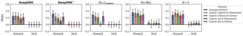
In this section, we perform ablation study on different terms introduced in Section 3.1.1, to show the necessity of designing these terms during the optimization for knockoffs. We consider the fully synthetic setup described in Section 4.3, and consider 200 and 2000 different sample sizes. The distribution for is . Overall, we consider the following terms and provide results in the associated tables: 1. REx; 2. the number of swappers ; 3. ; 4. the dependency regularized perturbation (denoted as ). Five synthetic datasets are considered as before and we report “FDR/power" values for each setup. We present results in Figure 9.
From Figure 9, we clearly observe that the defect of applying only one swapper or applying multiple swappers without considering or REx. They fail to control the FDR on all cases. The REx term is also crucial as it guarantees the adversarial environment created by different swappers are simultaneously resolved. In the figure, the importance is reflected by the increased FDR in the "No REx" case. is also a contributing term as essentially it guarantees the adversarial environments are not repetitive. Without this term we observe increment in FDR as compared to DeepDRK or . The comparison between DeepDRK and are subtle as has already obtained the knockoff of high quality. However, we empirically observe that adding the perturbation further increases the power for some datasets without sacrificing the FDR controllability. And for the case of mixture of Gaussian, it further helps to decorrelate features for a lower FDR. To interpret these observations, we follow a similar procedure in Section 4.3 to study the distribution of the knockoff statistics. Results are included in Section J.3 for consistency.
DeepDRK Deep Knockoff sRMMD KnockoffGAN DDLK
Overall, we verify that all terms are necessary components to achieve higher powers and controlled FDRs through this ablation study.
J.3 Analysis on the distribution of knockoff statistics
We present results of the distributions for both null and nonnull statistics on various experimental setups that are deferred from the main paper.
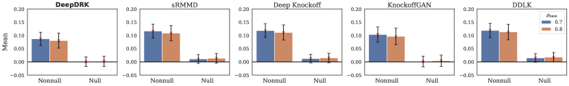
First, we present the distribution plot for the comparison on different benchmarking models and datasets in Figure 10. This complements the FDR-power figure (Figure 2) and the 200-sample-size figure (Figure 4) in the main paper. We notice that all models have concentrated null features around zero and relatively high values for the nonnull statistics for the case with 2000 samples. This corresponds to consistently well-performed FS results across all models and datasets, as shown in Figure 2.

Second, we present the distribution plot for the mixture of Gaussian data with increased correlation on the input features in both Figure 11 and Figure 12 for 200 and 2000 sample sizes, respectively. The figures complement to the FDR-power result in Figure 3. It is clear for both 200 and 2000 cases, all models experience increment in FDR and decrement in power. This phenomenon can be reflected by the increased positive shifts for the null features in Figure 11 and Figure 12. However, DeepDRK, in comparison, greatly controls the shift, achieving the best result with the lowest FDRs and comparative powers.
Lastly, we compare the distribution of the knockoff statistics on the ablation study. This complement the study in Section J.2. The results for both 200 and 2000 sample size setups are in Figure 13 and Figure 14. In the figures, Although the null statistics for DeepDRK, and “No " models concentrate symmetrically around zero, the heights of the nonnull statistics for DeepDRK are the highest, resulting higher power. And because some nonnull statistics have small values for the and “No " cases, we also expect them to have larger FDRs (see Figure 9). On the other hand, compared to DeepDRK, the models of “No REx" and “" experience clear positive shifts for the null statistics, leading to higher FDRs during FS (see Figure 9).
Appendix K Model Runtime
We consider evaluating and comparing model training runtime in Table 5 with the (2000, 100) setup, as it is common in existing literature. Although DeepDRK is not the fastest among the compared models, the time cost—7.35 minutes—is still short, especially when the performance is taken into account.
Appendix L Preparation of the RNA Data
We first normalize the raw data to value range and then standardize it to have zero mean and unit variance. is synthesized according to . We consider two different ways of synthesizing . The first is similar to the previous setup in the full synthetic case with and . For the second, the response is generated following the expression:
| (29) |
where follows the standard normal distribution and the 20 covariates are sampled uniformly.
Appendix M Real Case Study
Here we provide the supplementary information for the experiments described in Section 4.5. In Table 6, we provide all the 47 referenced metabolites based on our comprehensive literature review. In Table 7, we provide the list of identified metabolites by each of the considered models. This table corresponds to Table 1 in the main paper that only include metabolites counts due to space limitation.
Reference Type Metabolite Source Meatbolite Source PubChem palmitate CID: 985 taurocholate CID: 6675 cholate CID: 221493 p-hydroxyphenylacetate CID: 127 linoleate CID: 5280450 deoxycholate CID: 222528 taurochenodeoxycholate CID: 387316 Publications 12.13-diHOME [8] dodecanedioate [8] arachidonate [8] eicosatrienoate [8, 6] eicosadienoate [8] docosapentaenoate [8, 6] taurolithocholate [8] salicylate [8] saccharin [8] 1.2.3.4-tetrahydro-beta-carboline-1.3-dicarboxylate [8] oleate [6] arachidate [6] glycocholate [6] chenodeoxycholate [6] phenyllactate [38, 31] glycolithocholate [6] urobilin [38, 47] caproate [38, 32] hydrocinnamate [38, 29] myristate [38, 18] adrenate [38, 35] olmesartan [38, 49] tetradecanedioate [57, 39] hexadecanedioate [57, 39] oxypurinol [9] porphobilinogen [40] caprate [54, 53] undecanedionate [32, 59] stearate [2, 6] oleanate [44] glycochenodeoxycholate [51] sebacate [32] nervonic acid [58] lithocholate [6] Preprints alpha-muricholate [41] tauro-alpha-muricholate/tauro-beta-muricholate [41] 17-methylstearate [41] myristoleate [41] taurodeoxycholate [41] ketodeoxycholate [41]
Metabolite DeepDRK Deep Knockoff sRMMD KnockoffGAN DDLK 12.13-diHOME 9.10-diHOME caproate hydrocinnamate mandelate 3-hydroxyoctanoate caprate indoleacetate 3-hydroxydecanoate dodecanoate undecanedionate myristoleate myristate dodecanedioate pentadecanoate hydroxymyristate palmitoleate palmitate tetradecanedioate 10-heptadecenoate 2-hydroxyhexadecanoate alpha-linolenate linoleate oleate stearate hexadecanedioate 10-nonadecenoate nonadecanoate 17-methylstearate eicosapentaenoate arachidonate eicosatrienoate eicosadienoate eicosenoate arachidate phytanate docosahexaenoate docosapentaenoate adrenate 13-docosenoate eicosanedioate oleanate masilinate lithocholate chenodeoxycholate deoxycholate hyodeoxycholate/ursodeoxycholate ketodeoxycholate alpha-muricholate cholate glycolithocholate glycochenodeoxycholate glycodeoxycholate glycoursodeoxycholate glycocholate taurolithocholate taurochenodeoxycholate taurodeoxycholate taurohyodeoxycholate/tauroursodeoxycholate tauro-alpha-muricholate/tauro-beta-muricholate taurocholate salicylate saccharin azelate sebacate carboxyibuprofen olmesartan 1.2.3.4-tetrahydro-beta-carboline-1.3-dicarboxylate 4-hydroxystyrene acetytyrosine alpha-CEHC carnosol oxypurinol palmitoylethanolamide phenyllactate p-hydroxyphenylacetate porphobilinogen urobilin nervonic acid oxymetazoline