Globally Convergent Distributed Sequential Quadratic Programming with Overlapping Decomposition and Exact Augmented Lagrangian Merit Function

Abstract

In this paper, we address the problem of solving large-scale graph-structured nonlinear programs (gsNLPs) in a scalable manner. GsNLPs are problems in which the objective and constraint functions are associated with a graph node, and they depend only on the variables of adjacent nodes. This graph-structured formulation encompasses various specific instances, such as dynamic optimization, PDE-constrained optimization, multi-stage stochastic optimization, and optimization over networks. We propose a globally convergent overlapping graph decomposition method for solving large-scale gsNLPs under the standard regularity assumptions and mild conditions on the graph topology. At each iteration step, we use an overlapping graph decomposition to compute an approximate Newton step direction using parallel computations. We then select a suitable step size and update the primal-dual iterates by performing backtracking line search with the exact augmented Lagrangian merit function. By exploiting the exponential decay of sensitivity of gsNLPs, we show that the approximate Newton direction is a descent direction of the augmented Lagrangian merit function, which leads to global convergence and fast local convergence. In particular, global convergence is achieved for sufficiently large overlaps, and the local linear convergence rate improves exponentially in terms of the overlap size. This result matches existing results for dynamic programs. We validate our theory with an elliptic PDE-constrained problem.

1 Introduction

We consider graph-structured nonlinear programs (gsNLPs) [27]:

(1a) $$\min_{\{\boldsymbol{x}_{i}\in\mathbb{R}^{r_{i}}\}_{i\in\mathcal{V}}}\quad \sum_{i\in\mathcal{V}}f_{i}(\{\boldsymbol{x}_{j}\}_{j\in N_{\mathcal{G}}[i]}),$$

(1b) s.t. $$\boldsymbol{c}_{i}(\{\boldsymbol{x}_{j}\}_{j\in N_{\mathcal{G}}[i]})=\textbf{0},\;\;i\in\mathcal{\mathcal{V}},(\boldsymbol{\lambda}_{i}).$$

Here, $\mathcal{G}=(\mathcal{V},\mathcal{E})$ is an undirected graph; $\mathcal{V}$ is a strictly ordered node set; $\mathcal{E}\subseteq\{\{i,j\}\subseteq\mathcal{V}:i\neq j\}$ is the edge set; $N_{\mathcal{G}}[i]:=\{j\in\mathcal{V}:\{i,j\}\in\mathcal{E}\}\cup\{i\}$ is the closed neighborhood of $i\in\mathcal{V}$ on $\mathcal{G}$; $\boldsymbol{x}_{i}\in\mathbb{R}^{r_{i}}$ is the primal variable of node $i$; $f_{i}:\Pi_{j\in N_{\mathcal{G}}[i]}\mathbb{R}^{r_{j}}\rightarrow\mathbb{R}$ is the objective function of node $i$; $\boldsymbol{c}_{i}:\Pi_{j\in N_{\mathcal{G}}[i]}\mathbb{R}^{r_{j}}\rightarrow\mathbb{R}^{m_{i}}$ is the equality constraint function of node $i$; and $\boldsymbol{\lambda}_{i}\in\mathbb{R}^{m_{i}}$ are the variables of node $i$. These problems arise in various applications, including optimal control [4, 5], multi-stage stochastic optimization problems [18, 24], partial differential equations (PDEs) constrained problems [6], and network optimization [33].

In this paper, we study a scalable solution method for the large-scale instances of Eq. 1. The complexity of these problems arises from the large size of graph, which can render centralized solution methods intractable. To mitigate this, decomposition methods are employed. In these methods, the intractable full problem is decomposed into a set of smaller subproblems. These subproblems are designed to be individually tractable, and decomposition algorithms employ an iterative scheme that facilitates the convergence of the iterates towards the full solution. The convergence can be achieved through the exchange of solution information across the subproblems in each iteration step. Examples of decomposition algorithms include temporal decomposition [15, 31], Lagrangian decomposition [15, 2], Jacobi/Gauss-Seidel methods [32], and alternating direction method of multipliers (ADMM) [13]. Decomposition algorithms offer several advantages over centralized methods, including computational scalability and flexibility in implementation.

However, it is worth noting that decomposition algorithms are known to exhibit slower convergence rates compared to centralized methods [16]. This slower convergence can be attributed to the iterative nature of decomposition schemes and limited amount of information being shared across the subproblems. As demonstrated in the benchmark study [16], the practically observed convergence rate of conventional decomposition schemes is often too slow to be practically useful. Such limitations of the existing decomposition algorithms motivate the study of new decomposition algorithms that can overcome the slow convergence issue of conventional decomposition methods, while preserving its desired scalability.

In the recent line of work on overlapping decomposition [29, 26, 21, 22], the overlap has been exploited to improve the convergence behavior of decomposition algorithms. This method decomposes the original problem into a set of overlapping subproblems, and these subproblems are iteratively solved to promote the convergence to the full solution. The overlapping Schwarz method is one of the algorithms that utilize this type of overlapping decomposition strategy. The origin of this method traces back to the classical domain decomposition methods, which were originally developed for solving second-order elliptic partial differential equations [11, 10]. Recently, this scheme was adapted for structured optimization problems, and its convergence properties have been studied in different settings, including convex unconstrained quadratic programs [29], constrained quadratic programs [26], nonlinear optimal control [22], and general nonlinear optimization problems [25]. In these works, authors have established not only the convergence of these algorithms, but also the relationship between the convergence rate and the size of overlap. Specifically, they have shown that the (local) convergence rate improves exponentially with respect to the size of overlap, meaning that one can address the slow convergence issue of the decomposition methods by slightly increasing the subproblem complexity.

While the Schwarz scheme resolves the main issue of the conventional decomposition schemes, the Schwarz method does not employ sophisticated globalization strategies, such as merit function or filter, to enforce the global convergence. In particular, the previous works on the Schwarz schemes only guarantee the local convergence, meaning that it occurs with certainty only when the initial guess is sufficiently close to the local solutions. This limitation motivates the design of an enhanced algorithm, equipped with a globalization strategy to enforce the global convergence, while preserving the desired fast local convergence of the Schwarz schemes with overlap. This has motivated applying the overlapping decomposition within a well-established nonlinear optimization algorithm, in particular, within the sequential quadratic programming (SQP) method. In a recent work [21], authors have designed a so-called fast overlapping temporal decomposition (FOTD) procedure for the nonlinear equality-constrained dynamic problems (NLDPs). This method embeds the decomposition procedure into the sequential quadratic programming (SQP) framework and employes exact augmented Lagrangian merit function, which is defined as the summation of the Lagrangian function and the quadratic regularizations of primal and dual residuals to the stationarity conditions [19]. They have shown that this algorithm enjoys global convergence while preserving the desired fast local convergence of the Schwarz schemes.

Given the promising results of FOTD for dynamic programs, we aim to extend this result to a more general class of nonlinear programs. In particular, we design an algorithm that can handle the gsNLPs in the form of Eq. 1. To achieve global convergence, we employ the SQP-based strategy used in [21]. Specifically, we apply SQP with the exact augmented Lagrangian merit function to select the step size. To compute the SQP search direction, which is the computational bottleneck in the SQP method, we use the overlapping graph decomposition (OGD) strategy to solve the Newton system in a decomposed manner. Our main technical contribution is on showing the local and global convergence for the FOGD algorithm. To the best of our knowledge, our method is the first overlapping decomposition paradigm that can solve gsNLPs with a global convergence guarantee.

The remainder of this paper is organized as follows: In Section 2, we introduce SQP and OGD, and propose the FOGD procedure. In Section 3, we establish bounds to the error of the approximated Newton direction. In Section 4, we prove the global convergence of FOGD. In Section 5, we prove the local linear convergence of FOGD and establish the relationship between the convergence rate and size of overlap. In Section 6, we perform numerical experiments to demonstrate our theoretical findings. In Section 7, we conclude with some potential directions for future work. Some of the proofs are presented in the appendix to facilitate the reading.

Notations

For any integer $n$, $[n]:=\{1,\cdots,n\}$. Any vector $\boldsymbol{x}_{j}$ is assumed to be a column vector and we define $\{\boldsymbol{x}_{j}\}_{j\in\mathcal{J}}=(\boldsymbol{x}_{j_{1}},\cdots,\boldsymbol{x}_{j_{|\mathcal{J}|}})=[\boldsymbol{x}_{j_{1}}^{T},\cdots,\boldsymbol{x}_{j_{|\mathcal{J}|}}^{T}]^{T}$ where $\mathcal{J}=\{j_{1},j_{2},\cdots,j_{|\mathcal{J}|}\}$ with $j_{1}<j_{2}<\cdots<j_{|\mathcal{J}|}$. For matrices $M$, $M^{*}:=M[\mathcal{I}][\mathcal{J}]$ represents that $M^{*}$ is the submatrix of $M$ where ${M^{*}}_{i^{\prime},j^{\prime}}=M_{i_{i^{\prime}},j_{j^{\prime}}}$, $1\leq i^{\prime}\leq|\mathcal{I}|$, $1\leq j^{\prime}\leq|\mathcal{J}|$, $\mathcal{I}=\{i_{1},i_{2},\cdots,i_{|\mathcal{I}|}\}$ with $i_{1}<i_{2}<\cdots<i_{|\mathcal{I}|}$, and $\mathcal{J}=\{j_{1},j_{2},\cdots,j_{|\mathcal{J}|}\}$ with $j_{1}<j_{2}<\cdots<j_{|\mathcal{J}|}$. For any set $E$, we denote $|E|$ as the number of elements in $E$. For any two sets $E_{1}$ and $E_{2}$, $E_{1}\setminus E_{2}:=\{i:i\in E_{1},\;i\notin E_{2}\}$. Given the undirected graph $\mathcal{G}=(\mathcal{V},\mathcal{E})$ and node $i\in\mathcal{V}$, $N_{\mathcal{G}}(i):=N_{\mathcal{G}}[i]\setminus i$, and $N^{b}_{\mathcal{G}}[\mathcal{W}]:=\{j\in\mathcal{V}:d_{\mathcal{G}}(j,\mathcal{W})\leq b\}$ is the $b$-hop neighborhood of $\mathcal{W}\subseteq\mathcal{V}$ on $\mathcal{G}$ where we omit the superscript $b$ when $b=1$ e.g. $N_{\mathcal{G}}[\mathcal{W}]=N^{1}_{\mathcal{G}}[\mathcal{W}]$.

2 FOGD Algorithm Description

We present the FOGD algorithm in three steps: (1) Describe the Newton system required at every SQP iteration. (2) Explain how to apply OGD to solve the Newton system in step 1. (3) Introduce the merit function for selecting the step size and updating the iterate. (4) Summarize the full algorithm in Algorithm 1.

Step 1: Newton system of each SQP iteration

The Newton system in SQP is derived from the KKT condition of the Lagrangian function of Eq. 1. We define the Lagrangian function of Eq. 1 as $\mathcal{L}(\boldsymbol{x},\boldsymbol{\lambda})=f(\boldsymbol{x})+\boldsymbol{\lambda}^{T}\boldsymbol{c}(\boldsymbol{x})$ where $f(\boldsymbol{x})=\underset{i\in\mathcal{V}}{\sum}f_{i}(\{\boldsymbol{x}_{j}\}_{j\in N_{\mathcal{G}}[i]})$, $\boldsymbol{c}(\boldsymbol{x})=\{\boldsymbol{c}_{i}(\{\boldsymbol{x}_{j}\}_{j\in N_{\mathcal{G}}[i]})\}_{i\in\mathcal{V}}$, and $N$ represents the number of nodes in $\mathcal{V}$. We apply Newton’s method to the KKT conditions $\nabla_{\boldsymbol{x}}\mathcal{L}(\boldsymbol{x^{*}},\boldsymbol{\lambda^{*}})=\boldsymbol{0}$ and $\nabla_{\boldsymbol{\lambda}}\mathcal{L}(\boldsymbol{x^{*}},\boldsymbol{\lambda^{*}})=\boldsymbol{0}$ . The search direction $(\Delta\boldsymbol{x}^{\tau},\Delta\boldsymbol{\lambda}^{\tau})$ at the $\tau$-th iteration is obtained by solving the following Newton-KKT system

(2) $$\begin{pmatrix}\hat{H}^{\tau}&(G^{\tau})^{T}\\ G^{\tau}&\boldsymbol{0}\\ \end{pmatrix}\begin{pmatrix}\Delta\boldsymbol{x}^{\tau}\\ \Delta\boldsymbol{\lambda}^{\tau}\\ \end{pmatrix}=-\begin{pmatrix}\nabla_{\boldsymbol{x}}\mathcal{L}^{\tau}\\ \nabla_{\boldsymbol{\lambda}}\mathcal{L}^{\tau}\\ \end{pmatrix},$$

where $\nabla_{\boldsymbol{x}}\mathcal{L}^{\tau}=\nabla_{\boldsymbol{x}}\mathcal{L}(\boldsymbol{x}^{\tau},\boldsymbol{\lambda}^{\tau})$, $\nabla_{\boldsymbol{\lambda}}\mathcal{L}^{\tau}=\nabla_{\boldsymbol{\lambda}}\mathcal{L}(\boldsymbol{x}^{\tau},\boldsymbol{\lambda}^{\tau})$, $\hat{H}^{\tau}$ is a modified Hessian, and $G^{\tau}=\nabla_{\boldsymbol{x}}\boldsymbol{c}(\boldsymbol{x}^{\tau})$.

Note that Eq. 2 is the KKT condition of the following quadratic program:

(3) $$\min_{\boldsymbol{\omega}}\;\; \frac{1}{2}\boldsymbol{\omega}^{T}\hat{H}^{\tau}\boldsymbol{\omega}+\boldsymbol{\omega}^{T}\nabla_{\boldsymbol{x}}\mathcal{L}^{\tau},\quad\text{s.t.}\;\; G^{\tau}\boldsymbol{\omega}+\boldsymbol{c}^{\tau}=\boldsymbol{0},\,(\boldsymbol{\zeta}).$$

where $\boldsymbol{c}^{\tau}=(\boldsymbol{c}^{\tau}_{1},\cdots,\boldsymbol{c}^{\tau}_{N})$ and $\boldsymbol{c}^{\tau}_{j}=\boldsymbol{c}_{j}(\boldsymbol{x}^{\tau})$ for $\forall j\in[N]$. Since Jacobian $G$ in Eq. 3 has full row rank in any iteration and $(Z^{\tau})^{T}\hat{H}^{\tau}(Z^{\tau})$ is positive definite, the solution of Eq. 2 is the unique global solution of Eq. 3 [23, Lemma 16.1]. Therefore, to obtain the solution of Eq. 2, we can solve Eq. 3 instead. For Eq. 3, we denote $\boldsymbol{\omega}$ and $\boldsymbol{\zeta}$ as the primal and dual variables respectively, $(\boldsymbol{\omega^{*}},\boldsymbol{\zeta^{*}})$ as the global solutions, and $(\Delta\boldsymbol{x},\Delta\boldsymbol{\lambda})=(\boldsymbol{\omega^{*}},\boldsymbol{\zeta^{*}})$.

Step 2: Apply OGD to solve the Newton System Eq. 2 approximately

Since we consider large-scale gsNLPs, solving Eq. 2 exactly can be computationally intractable. To overcome this issue, we apply OGD to Eq. 3 to compute an approximate solution of Eq. 2 at reduced computational cost. The OGD procedure can be summarized as follows. First, we consider a set of overlapping subdomains that jointly covers the entire problem domain $\mathcal{V}$. Over each subdomain we consider the associated objective and constraints to formulate a subproblem. Then, these subproblems are solved to optimality, and the internal solutions in each subdomain are concatenated to obtain the approximate search direction.

First, we explain how the set of overlapping subgraphs can be constructed. We first consider a partition $\{\mathcal{V}_{i}\}_{i\in[M]}$ of $\mathcal{V}$; i.e., $\bigcup_{i\in[M]}\mathcal{V}_{i}=\mathcal{V}$ and $\{\mathcal{V}_{i}\}_{i\in[M]}$ are nonempty, disjoint with each other. Then, we expand each $\mathcal{V}_{i}$ by a user-defined parameter $b\geq 1$ (called the size of overlap); that is, we choose $\{\mathcal{W}_{i}\subseteq\mathcal{V}\}_{i\in[M]}$ so that $N^{b}_{\mathcal{G}}[\mathcal{V}_{i}]\subseteq\mathcal{W}_{i},\;\forall i\in[M]$. In the simplest case, one may choose $\mathcal{W}_{i}=N^{b}_{\mathcal{G}}[\mathcal{V}_{i}]$.

We are ready to state subproblems $\mathcal{L}\mathcal{P}_{i}^{\mu}$ defined on each overlapping subdomain $\mathcal{W}_{i}$:

$$\min_{\boldsymbol{\tilde{\omega}}_{i}}\;\; \left(\nabla_{\boldsymbol{\widetilde{x}}_{i}}\mathcal{L}^{\tau}\right)^{T}\boldsymbol{\tilde{\omega}}_{i}+\frac{1}{2}\boldsymbol{\tilde{\omega}}_{i}^{T}\hat{H}^{\tau}[\mathcal{W}_{i}][\mathcal{W}_{i}]\boldsymbol{\tilde{\omega}}_{i}+\frac{\mu}{2}\bigg{\|}\nabla_{\boldsymbol{\widetilde{x}}_{i}}\boldsymbol{c}^{\tau}_{\hat{\mathcal{W}_{i}}}\boldsymbol{\tilde{\omega}}_{i}+\boldsymbol{c}^{\tau}_{\hat{\mathcal{W}_{i}}}\bigg{\|}^{2},$$

(4a) s.t. $$G^{\tau}[\mathcal{W}_{i}\setminus\tilde{\mathcal{W}}_{i}][\mathcal{W}_{i}]\boldsymbol{\tilde{\omega}}_{i}+\boldsymbol{c}^{\tau}[\mathcal{W}_{i}\setminus\tilde{\mathcal{W}}_{i}]=0,\quad(\boldsymbol{\tilde{\zeta}}_{i}).$$

where $\tilde{\mathcal{W}}_{i}$ is defined as $\tilde{\mathcal{W}}_{i}:={N_{\mathcal{G}}\left(N_{\mathcal{G}}(\mathcal{W}_{i})\right)}\cap\mathcal{W}_{i}$ (the internal boundary of $\mathcal{W}_{i}$), $\hat{\mathcal{W}_{i}}$ is defined as $\hat{\mathcal{W}_{i}}:=N_{\mathcal{G}}(\mathcal{W}_{i})\cup\tilde{\mathcal{W}}_{i}$ (the internal and external boundary of $\mathcal{W}_{i}$) , $\boldsymbol{\widetilde{x}}_{i}=\{\boldsymbol{x}_{j}\}_{j\in\mathcal{W}_{i}}$, $\boldsymbol{\tilde{\omega}}_{i}=\{\boldsymbol{\tilde{\omega}}_{i,j}\}_{j\in\mathcal{W}_{i}}$, and $\boldsymbol{\tilde{\zeta}}_{i}=\{\boldsymbol{\tilde{\zeta}}_{i,j}\}_{j\in\mathcal{W}_{i}\setminus\tilde{\mathcal{W}}_{i}}$. The perturbed version of Eq. 4 is established in Section 3, and the illustration of $\mathcal{V}_{i}$, $\mathcal{W}_{i}$, $\tilde{\mathcal{W}_{i}}$, $N_{\mathcal{G}}(\mathcal{W}_{i})$, and $\hat{\mathcal{W}_{i}}$ is given in Fig. 1. We denote $(\boldsymbol{\tilde{\omega}}_{i},\boldsymbol{\tilde{\zeta}}_{i})$ as primal and dual variables of $\mathcal{L}\mathcal{P}_{i}^{\mu}$, and $(\boldsymbol{\tilde{\omega}}_{i}^{*},\boldsymbol{\tilde{\zeta}}_{i}^{*})$ as the solution of $\mathcal{L}\mathcal{P}_{i}^{\mu}$.

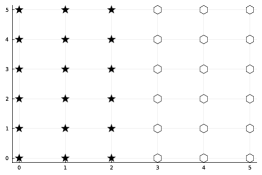
(a) $\mathcal{V}_{1}$, $\mathcal{V}_{2}$, and $\mathcal{V}$

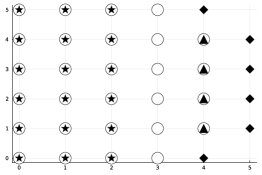
(b) $\mathcal{V}_{1}$, $\mathcal{W}_{1}$, $\tilde{\mathcal{W}_{1}}$, $N_{\mathcal{G}}(\mathcal{W}_{1})$, and $\hat{\mathcal{W}_{1}}$

Figure 1: The illustration of $\mathcal{V}_{i}$, $\mathcal{W}_{i}$, $\tilde{\mathcal{W}_{i}}$, $N_{\mathcal{G}}(\mathcal{W}_{i})$, and $\hat{\mathcal{W}_{i}}$. We consider a simple two-dimensional graph which is divided into two subgraphs with the size of overlap 2. In Fig. 1(a), star markers represent $\mathcal{V}_{1}$, hexagon markers represent $\mathcal{V}_{2}$, and $\mathcal{V}=\mathcal{V}_{1}\cup\mathcal{V}_{2}$. In Fig. 1(b), star markers represents $\mathcal{V}_{1}$, circle markers represent $\mathcal{W}_{1}$, triangle markers represent $\tilde{\mathcal{W}_{1}}$, diamond markers represent $N_{\mathcal{G}}(\mathcal{W}_{i})$, and circle, diamond markers represent $\hat{\mathcal{W}_{i}}$.

Note that in Eq. 4, only the internal constraints—the constraints that are only dependent on the variables in $\mathcal{W}_{i}$— are enforced as the constraints in the subproblem. The coupling constraints—the constraints that depend on the variables that are not associated with $\mathcal{W}_{i}$— are incorporated as augmented Lagrangain-like regularization terms. Later, we will see that such a treatment of the constraints allows for the subproblems to inherit the desired regularity conditions (uniform SOSC and LICQ conditions) from the full problem.

Based on the subproblem formulation in Eq. 4, one can apply the OGD to approximately solve Eq. 2 at every iteration. At $\tau$-th iteration, we first evaluate the Hessian matrix $\hat{H}^{\tau}$, Jacobian matrix $G^{\tau}$, the derivative of Lagrangian function $\nabla\mathcal{L}^{\tau}$, and the constraint vector $\boldsymbol{c}^{\tau}$ with the primal-dual variables $\boldsymbol{x}^{\tau}$ and $\boldsymbol{\lambda}^{\tau}$. The submatrix/subvector of these quantities can be later used for formulating the subproblems. Then, we specify the boundary parameters of each subproblem as zero vectors and solve the subproblem $\mathcal{L}\mathcal{P}_{i}^{\mu}$ defined in Eq. 4 to the optimality. Finally, for every subproblem $\mathcal{L}\mathcal{P}_{i}^{\mu}$, we only keep $\{\boldsymbol{\tilde{\omega}}^{\tau}_{j,k}\}_{k\in\mathcal{V}_{i}}$ and $\{\boldsymbol{\tilde{\zeta}}^{\tau}_{j,k}\}_{k\in\mathcal{V}_{i}}$ in the disjoint set $\mathcal{V}_{i}$ and concatenate them to obtain the approximated Newton search direction $(\tilde{\Delta}\boldsymbol{x}^{\tau},\tilde{\Delta}\boldsymbol{\lambda}^{\tau})$ at $\tau$-th iteration.

Step 3: Merit function, step size selection, and iterate update

After obtaining the approximated Newton search direction, it is necessary to choose an appropriate merit function to select step size and update iterates before entering the next iteration. We first introduce the definition of concatenation and decomposition, where we adapt the definition in [21] to our case and rewrite them as follows.

Definition 2.1.

(concatenation and decomposition). Given the $i$-th subproblem variables $\{(\boldsymbol{\tilde{\omega}}_{i},\boldsymbol{\tilde{\zeta}}_{i})\}_{i=1}^{M}$, we define the concatenation operator $\mathcal{C}$ as $\mathcal{C}(\{(\boldsymbol{\tilde{\omega}}_{i},\boldsymbol{\tilde{\zeta}}_{i})\}_{i=1}^{M})=(\boldsymbol{\omega},\boldsymbol{\zeta})$, where $(\boldsymbol{\omega}_{k},\boldsymbol{\zeta}_{k})=(\boldsymbol{\tilde{\omega}}_{i,k},\boldsymbol{\tilde{\zeta}}_{i,k})$ if $k\in\mathcal{V}_{i}$. Conversely, given a full-domain variable $(\boldsymbol{\omega},\boldsymbol{\zeta})$, we define the decomposition operator $\mathcal{C}^{-1}$ as

(5) $$\mathcal{C}^{-1}(\boldsymbol{\omega},\boldsymbol{\zeta})=\{\mathcal{C}^{-1}_{i}(\boldsymbol{\omega},\boldsymbol{\zeta})\}_{i=1}^{M},\quad\mathcal{C}^{-1}_{i}(\boldsymbol{\omega},\boldsymbol{\zeta})=(\boldsymbol{\tilde{\omega}}_{i},\boldsymbol{\tilde{\zeta}}_{i}).$$

At $\tau$-th iteration, we concatenate the solution of subproblems $\mathcal{L}\mathcal{P}^{\mu}_{i}$ to obtain an approximated Newton’s direction $(\tilde{\Delta}\boldsymbol{x}^{\tau},\tilde{\Delta}\boldsymbol{\lambda}^{\tau})=\mathcal{C}(\{(\boldsymbol{\tilde{\omega}}_{i}^{*},\boldsymbol{\tilde{\zeta}}_{i}^{*})\}_{i=1}^{M})$. With $(\tilde{\Delta}\boldsymbol{x}^{\tau},\tilde{\Delta}\boldsymbol{\lambda}^{\tau})$, we update the primal-dual variables of the full problem Eq. 1 with

(6) $$\begin{pmatrix}\boldsymbol{x}^{\tau+1}\\ \boldsymbol{\lambda}^{\tau+1}\end{pmatrix}=\begin{pmatrix}\boldsymbol{x}^{\tau}\\ \boldsymbol{\lambda}^{\tau}\end{pmatrix}+\alpha^{\tau}\begin{pmatrix}\tilde{\Delta}\boldsymbol{x}^{\tau}\\ \tilde{\Delta}\boldsymbol{\lambda}^{\tau}\end{pmatrix},$$

where the choice of the stepsize $\alpha^{\tau}$ is based on the Armijo condition and the following differentiable exact augmented Lagrangian merit function

(7) $$\mathcal{L}_{\eta}(\boldsymbol{x},\boldsymbol{\lambda})=\mathcal{L}(\boldsymbol{x},\boldsymbol{\lambda})+\frac{\eta_{1}}{2}\|\nabla_{\boldsymbol{\lambda}}\mathcal{L}(\boldsymbol{x},\boldsymbol{\lambda})\|^{2}+\frac{\eta_{2}}{2}\|\nabla_{\boldsymbol{x}}\mathcal{L}(\boldsymbol{x},\boldsymbol{\lambda})\|^{2},$$

with penalty parameters $\eta=(\eta_{1},\eta_{2})$ where $\eta_{1}$ and $\eta_{2}$ penalize the error of feasibility and optimality respectively. We can show that solving the unconstrained problem $\underset{\boldsymbol{x},\boldsymbol{\lambda}}{\min}\;\mathcal{L}_{\eta}(\boldsymbol{x},\boldsymbol{\lambda})$ with large enough $\eta_{1}$ and small enough $\eta_{2}$ is equivalent to solving Eq. 1, by [3, Proposition 4.15]. While many choices of merit functions exist for the SQP-based algorithms, the exact augmented Lagrangian function Eq. 7 fits our algorithm and analysis better for the following reasons. First, we require the merit function to undergo the perturbation of dual variables of Eq. 1, since the formulation of the subproblem $\mathcal{L}\mathcal{P}_{i}^{\mu}$ depends on these dual variables through the Lagrangian. This requirement excludes the merit functions that solely include the primal variables of Eq. 1. Second, the differentiability of Eq. 7 allows us to use a simple backtracking line search without facing the Maratos effect. More discussion of Eq. 7 will come later.

With the merit function Eq. 7, we choose the stepsize $\alpha_{\tau}>0$ according to the Armijo condition as follows

(8) $$\mathcal{L}_{\eta}^{\tau+1}\leq\mathcal{L}_{\eta}^{\tau}+\beta_{1}\,\alpha_{\tau}\,\begin{pmatrix}\nabla_{\boldsymbol{x}}\mathcal{L}_{\eta}^{\tau}\\ \nabla_{\boldsymbol{\lambda}}\mathcal{L}_{\eta}^{\tau}\end{pmatrix}^{T}\begin{pmatrix}\tilde{\Delta}\boldsymbol{x}^{\tau}\\ \tilde{\Delta}\boldsymbol{\lambda}^{\tau}\end{pmatrix},$$

where the predetermined parameter $\beta_{1}\in(0,\frac{1}{2})$, $\mathcal{L}_{\eta}^{\tau}=\mathcal{L}_{\eta}(\boldsymbol{x}^{\tau},\boldsymbol{\lambda}^{\tau})$ (similar definitions hold for $\mathcal{L}_{\eta}^{\tau+1}$ and $\nabla\mathcal{L}_{\eta}^{\tau}$), and

(9) $$\begin{pmatrix}\nabla_{\boldsymbol{x}}\mathcal{L}_{\eta}(\boldsymbol{x},\boldsymbol{\lambda})\\ \nabla_{\boldsymbol{\lambda}}\mathcal{L}_{\eta}(\boldsymbol{x},\boldsymbol{\lambda})\end{pmatrix}=\begin{pmatrix}(I+\eta_{2}H(\boldsymbol{x},\boldsymbol{\lambda}))\nabla_{\boldsymbol{x}}\mathcal{L}(\boldsymbol{x},\boldsymbol{\lambda})+\eta_{1}G^{T}(\boldsymbol{x})\nabla_{\boldsymbol{\lambda}}\mathcal{L}(\boldsymbol{x},\boldsymbol{\lambda})\\ \eta_{2}G(\boldsymbol{x})\nabla_{\boldsymbol{x}}\mathcal{L}(\boldsymbol{x},\boldsymbol{\lambda})+\nabla_{\boldsymbol{\lambda}}\mathcal{L}(\boldsymbol{x},\boldsymbol{\lambda})\end{pmatrix}.$$

A standard backtracking line search procedure (e.g., halving the candidate step size until the conditions Eq. 8 and Eq. 9 are satisfied) can be applied to find such $\alpha_{\tau}$.

We now summarize the complete FOGD algorithm in Algorithm 1 where $M$ represents the number of subproblems. In the next section, we will study the difference between the approximated Newton direction $(\tilde{\Delta}\boldsymbol{x}^{\tau},\tilde{\Delta}\boldsymbol{\lambda}^{\tau})$ and the exact Newton direction $(\Delta\boldsymbol{x}^{\tau},\Delta\boldsymbol{\lambda}^{\tau})$.

Algorithm 1 A Fast Overlapping Graph Decomposition Procedure

1:Input : initial iterate $(\boldsymbol{x}^{0},\boldsymbol{\lambda}^{0})$, scalars $\mu,\,\eta_{1},\,\eta_{2}>0,\,\beta_{1}\in(0,1/2)$;

2:for $\tau=0,1,2,\cdots$ do

3:     Compute $\hat{H}^{\tau},G^{\tau},$ and $\nabla\mathcal{L}^{\tau}$;

4:     for $i=0,1,\cdots,M-1\cdots$ (in parallel) do

5:         Solve $\mathcal{L}\mathcal{P}_{i}^{\mu}$ in Eq. 4 to obtain solution $(\boldsymbol{\tilde{\omega}}_{i}^{*},\boldsymbol{\tilde{\zeta}}_{i}^{*})$;

6:     end for

7:     Let $(\tilde{\Delta}\boldsymbol{x}^{\tau},\tilde{\Delta}\boldsymbol{\lambda}^{\tau})=\mathcal{C}(\{(\boldsymbol{\tilde{\omega}}_{i}^{*},\boldsymbol{\tilde{\zeta}}_{i}^{*})\}_{i=1}^{M})$;

8:     Select $\alpha_{\tau}$ by Eq. 8 and update iterate by Eq. 6;

9:end for

3 Error Analysis of OGD

In the previous section, we have described how to approximate the Newton direction by OGD for every SQP iteration. A natural question here is how well the approximated search direction estimates the exact search direction. In this section, we will answer it by giving an upper bound for $(\tilde{\Delta}\boldsymbol{x}^{\tau}-\Delta\boldsymbol{x}^{\tau},\tilde{\Delta}\boldsymbol{\lambda}^{\tau}-\Delta\boldsymbol{\lambda}^{\tau})$ where $(\tilde{\Delta}\boldsymbol{x}^{\tau},\tilde{\Delta}\boldsymbol{\lambda}^{\tau})$ is the approximated Newton direction obtained by OGD and $(\Delta\boldsymbol{x}^{\tau},\Delta\boldsymbol{\lambda}^{\tau})$ is the exact Newton direction.

We first introduce the perturbed version of Eq. 4 where $\boldsymbol{d}_{i}$ is the boundary parameter of $\mathcal{L}\mathcal{P}_{i}^{\mu}(\boldsymbol{d}_{i})$ and $\boldsymbol{d}_{i}$ might not be a zero vector. Recall, the variables $\boldsymbol{\tilde{\omega}}_{i}$ are attached to the overlapping domain $\mathcal{W}_{i}$.

(10a) $$\min_{\boldsymbol{\tilde{\omega}}_{i}}\;\; \left(\nabla_{\boldsymbol{\widetilde{x}}_{i}}\mathcal{L}^{\tau}\right)^{T}\boldsymbol{\tilde{\omega}}_{i}+\frac{1}{2}\hat{\boldsymbol{\omega}}^{T}\hat{H}^{\tau}\hat{\boldsymbol{\omega}}+{\color[rgb]{1,.5,0}\boldsymbol{\bar{\zeta}}_{\hat{\mathcal{W}_{i}}}}^{T}\nabla_{\boldsymbol{\widetilde{x}}_{i}}\boldsymbol{c}^{\tau}_{\hat{\mathcal{W}_{i}}}\boldsymbol{\tilde{\omega}}_{i}+\frac{\mu}{2}\bigg{\|}\left(\nabla_{\boldsymbol{x}}\boldsymbol{c}^{\tau}\hat{\boldsymbol{\omega}}+\boldsymbol{c}^{\tau}\right)_{\hat{\mathcal{W}_{i}}}\bigg{\|}^{2},$$

(10b) s.t. $$G^{\tau}[\mathcal{W}_{i}\setminus\tilde{\mathcal{W}}_{i}][\mathcal{W}_{i}]\boldsymbol{\tilde{\omega}}_{i}+\boldsymbol{c}^{\tau}[\mathcal{W}_{i}\setminus\tilde{\mathcal{W}}_{i}]=0,\quad(\boldsymbol{\tilde{\zeta}}_{i}).$$

where the boundary variable $\boldsymbol{d}_{i}$ is given as $\boldsymbol{d}_{i}=\left((\boldsymbol{\bar{\omega}}_{j})_{j\in\mathcal{W}_{p_{i}}},(\boldsymbol{\bar{\zeta}}_{j})_{j\in\hat{\mathcal{W}_{i}}}\right)$, $\mathcal{W}_{p_{i}}=N_{\mathcal{G}}(\mathcal{W}_{i})\cup N_{\mathcal{G}}\left(N_{\mathcal{G}}[\mathcal{W}_{i}]\right)$ (the external boundary of depth two of $\mathcal{W}_{i}$), $\hat{\boldsymbol{\omega}}=\{\boldsymbol{\tilde{\omega}}_{i,j}\}_{j\in\mathcal{W}_{i}}\cup\{\boldsymbol{\bar{\omega}}_{j}\}_{j\in\mathcal{V}\setminus\mathcal{W}_{i}}$, and $\boldsymbol{\bar{\omega}}$, $\boldsymbol{\bar{\zeta}}$ are specified by the boundary variable $\boldsymbol{d}_{i}$. We denote $\boldsymbol{\tilde{\omega}}_{i}(\boldsymbol{d}_{i})=\{\boldsymbol{\tilde{\omega}}_{i,j}\}_{j\in\mathcal{W}_{i}}$, $\boldsymbol{\tilde{\zeta}}_{i}(\boldsymbol{d}_{i})=\{\boldsymbol{\tilde{\zeta}}_{i,j}\}_{j\in\mathcal{W}_{i}\setminus\tilde{\mathcal{W}}_{i}}$ as primal and dual variables of $\mathcal{L}\mathcal{P}_{i}^{\mu}(\boldsymbol{d}_{i})$, and $(\boldsymbol{\tilde{\omega}}_{i}^{*}(\boldsymbol{d}_{i}),\boldsymbol{\tilde{\zeta}}_{i}^{*}(\boldsymbol{d}_{i}))$ as the solution of $\mathcal{L}\mathcal{P}_{i}^{\mu}(\boldsymbol{d}_{i})$. Note that $\mathcal{L}\mathcal{P}_{i}^{\mu}(\boldsymbol{0})$ reduces to $\mathcal{L}\mathcal{P}_{i}^{\mu}$.

Then, we introduce several assumptions. Note that these assumptions explicitly introduce the constants that will be used for the subsequent error analysis. We emphasize that these parameters are assumed to be independent of other problem parameters, such as the size of graph $N$. [lower bound on the reduced Hessian] For any iteration $\tau\geq 0$, we let $Z^{\tau}$ be a matrix whose columns are orthonormal vectors that span the null space of $\{\omega:G^{\tau}\omega=0\}$. We assume that there exists a constant $\gamma_{RH}>0$ such that for all $\tau$,

(11) $$(Z^{\tau})^{T}\,\hat{H}^{\tau}(Z^{\tau})\succeq\gamma_{RH}I,$$

Note that the matrix on the left-hand side is called the reduced Hessian. [linear independence constraint qualification] There exists $\beta>0$ such that for all $\tau$, $G^{\tau}(G^{\tau})^{T}\succeq\beta I$. [L-uniformly bounded Lagrangian Hessian] There exists $L\geq 0$ such that $\max\left(\|\nabla_{\boldsymbol{q}\boldsymbol{q}}\tilde{\mathcal{L}}^{\tau}(\boldsymbol{x},\boldsymbol{\lambda})\|,\|\nabla_{\boldsymbol{q}\boldsymbol{\tilde{q}}}\tilde{\mathcal{L}}^{\tau}(\boldsymbol{x},\boldsymbol{\lambda})\|,\|H^{\tau}\|,\max_{k\in\mathcal{V},l\in[m_{k}]}\left(\|\nabla_{\boldsymbol{x},\boldsymbol{x}}c_{k,l}\|\right)\right)\leq L$, where $\boldsymbol{q}$ and $\boldsymbol{\tilde{q}}$ are primal-dual variables and data of Eq. 3, and $\tilde{\mathcal{L}}$ is the Lagrange function of Eq. 3. There exist polynomial functions $C^{*}(\cdot)$ and $e(\cdot)$ such that

(12a) $$d_{\mathcal{G}}(k,j) \leq C^{*}(b),\quad\forall k,j\in\mathcal{W}_{i},\;i\in[M]$$

(12b) $$|\{j\in\mathcal{V}:d_{\mathcal{G}}(i,j)\leq d\}| \leq e(d),\quad\forall i\in\mathcal{V}.$$

We require Assumptions 3-11 to hold for Eq. 3 to guarantee that there exists a unique solution of Eq. 3. Also, they play important roles in establishing lemmas and theorem in Section 3 and they are standard assumptions in SQP literature [14, 8, 17]. Assumption 11 is useful when proving that the reduced Hessian matrices of the subproblems $\{\mathcal{L}\mathcal{P}_{i}^{\mu}\}_{i\in[M]}$ are positive definite. Assumption 3 introduces mild conditions on the graph topology, which is designed to help establish the uniform bound in Theorem 3.9. In particular, (12a) ensures that the diameter of each overlapping subdomain is bounded by a polynomial of the size of overlap, and (12b) ensures that the graph is growing polynomially. With the fixed graph size $N$, it is clear that Assumption 11 holds since the objective function $f_{i}$ and constraint function $\boldsymbol{c}_{i}$ are twice continuously differentiable. Assumption 3 is adapted from [28, Assumption 3.4]. Given the above assumptions, we are able to establish the existence and uniqueness of the solution to subproblems $\mathcal{L}\mathcal{P}_{i}^{\mu}(\boldsymbol{d}_{i})$ in the following lemma.

Lemma 3.1.

Suppose Assumptions 3-3 hold for Problem Eq. 3. Then, for all subproblems $\{\mathcal{L}\mathcal{P}_{i}^{\mu}(\boldsymbol{d}_{i})\}_{i\in[M]}$ in Eq. 10 with any boundary variables $\boldsymbol{d}_{i}$ and $\mu\geq\bar{\mu}:=(2L^{2}/\gamma_{RH}+\gamma_{RH}+L)/\beta$, LICQ holds and its reduced Hessian matrix is lower bounded by $(\gamma_{RH}/2)I$ at any iteration $\tau\geq 0$. This implies that $\mathcal{L}\mathcal{P}_{i}^{\mu}(\boldsymbol{d}_{i})$ has a unique global solution.

Proof 3.2.

See Section A.1.

Lemma 3.1 shows that the LICQ and SSOSC hold for $\mathcal{L}\mathcal{P}_{i}^{\mu}(\boldsymbol{d}_{i})$ for any boundary variables $\boldsymbol{d}_{i}$ and $\mu\geq\bar{\mu}$. It also implies that the uniqueness and existence of the solution to $\mathcal{L}\mathcal{P}_{i}^{\mu}(\boldsymbol{d}_{i})$ does not depend on $\boldsymbol{d}_{i}$. Also, it shows that subproblems enjoy similar properties as the full problems and enables us to prove the exponential decay property of the KKT inverse matrix of subproblems, which is our main tool when analyzing the approximation error of search directions. The next lemma aims to establish the exponential decay property of the inverse of the KKT matrix, which plays a key role in proving Lemma 3.7. We note that [20, Lemma 2] established the decay result for optimal control problems (i.e., linear graphs), while we consider here a more general graph. We first introduce the definition of the inverse of the KKT matrix.

We define the KKT matrix for $\mathcal{L}\mathcal{P}_{i}^{\mu}$ evaluated at $(\boldsymbol{x},\boldsymbol{\lambda})$ by

(13) $$K_{i}(\boldsymbol{x},\boldsymbol{\lambda})=\begin{bmatrix}\hat{H}^{\mu}_{i}&(G_{i})^{T}\\ G_{i}&\boldsymbol{0}\\ \end{bmatrix}$$

Its inverse is partitioned as

(14) $$K_{i}^{-1}(\boldsymbol{x},\boldsymbol{\lambda})=\begin{bmatrix}K_{i,{\color[rgb]{0,0,0}\{(k,j)\}},1}^{-1}&K_{i,{\color[rgb]{0,0,0}\{(k,j_{1})\}},2}^{-1}\\ K_{i,{\color[rgb]{0,0,0}\{(k,j_{1})\}},2}^{-1\quad T}&K_{i,{\color[rgb]{0,0,0}\{(k_{1},j_{1})\}},3}^{-1}\\ \end{bmatrix}$$

where $\forall k,j\in\mathcal{W}_{i}$, $\forall k_{1},j_{1}\in\mathcal{W}_{i}\setminus\tilde{\mathcal{W}}_{i}$, $G_{i}=G[\mathcal{W}_{i}\setminus\tilde{\mathcal{W}}_{i}][\mathcal{W}_{i}]$, $\hat{H}^{\mu}_{i}$ represents the Hessian matrix of Eq. 10, $K_{i,(k,j),1}^{-1}\in\mathbb{R}^{r_{k}\times r_{j}}$ is the block corresponding to node $k$ in the row and node $j$ in the column. Similarly, $K_{i,(k,j_{1}),2}^{-1}\in\mathbb{R}^{r_{k}\times m_{j_{1}}}$, and $K_{i,(k_{1},j_{1}),3}^{-1}\in\mathbb{R}^{m_{k_{1}}\times m_{j_{1}}}$.

We now characterize the structure of $K_{i}^{-1}$.

Lemma 3.3 (Structure of KKT inverse).

For any point $(\boldsymbol{x},\boldsymbol{\lambda})$ such that Assumptions 3-3 hold for the full problem Eq. 3, we have

(15a) $$\|K_{i,(k,j),1}^{-1}\| \leq\hat{\gamma}\rho^{d_{\mathcal{G}}(k,j)} \quad k,j\in\mathcal{W}_{i}$$

(15b) $$\|K_{i,(k,j_{1}),2}^{-1}\| \leq\hat{\gamma}\rho^{d_{\mathcal{G}}(k,j_{1})} \quad k\in\mathcal{W}_{i},j_{1}\in\mathcal{W}_{i}\setminus\tilde{\mathcal{W}}_{i}$$

(15c) $$\|K_{i,(k_{1},j_{1}),3}^{-1}\| \leq\hat{\gamma}\rho^{d_{\mathcal{G}}(k_{1},j_{1})} \quad k_{1},j_{1}\in\mathcal{W}_{i}\setminus\tilde{\mathcal{W}}_{i}$$

where $\gamma_{H}=\left(\frac{4}{\gamma_{RH}}+\left(1+\frac{8L}{\gamma_{RH}}+\frac{16L^{2}}{\gamma_{RH}^{2}}\right)\frac{L(1+\mu^{*}L)}{\beta}+\mu^{*}\right)^{-1}$, $\mu^{*}=\frac{8L^{2}/\gamma_{RH}+\gamma_{RH}+2L}{2\beta}$, $\rho=\left(\frac{L^{2}-\gamma_{H}^{2}}{L^{2}+\gamma_{H}^{2}}\right)^{\frac{1}{2}}$, $\hat{\gamma}=\frac{L}{\gamma_{H}^{2}\rho}$.

Proof 3.4.

The lemma can be obtained directly from Lemma 3.1, [27,  Theorem 3.6], and [28,  Theorem A.3].

In Lemma 3.3, the block elements of subproblems’ KKT inverse matrices exhibit the exponential decay property. The norm of its $(i,j)$-th block decreases exponentially with the increase of $d_{\mathcal{G}}(i,j)$. This property will be useful for the proof of Lemma 3.7. Before introducing Lemma 3.7 to give an upper bound of $\|(\boldsymbol{\tilde{\omega}}^{*}_{i}(\boldsymbol{d}_{i}),\boldsymbol{\tilde{\zeta}}^{*}_{i}(\boldsymbol{d}_{i}))-(\boldsymbol{\tilde{\omega}}^{*}_{i}(\boldsymbol{d^{\prime}}_{i}),\boldsymbol{\tilde{\zeta}^{*}}_{i}(\boldsymbol{d^{\prime}}_{i}))\|$, we still need a helper lemma which shows that the local solution of Eq. 3 is also a local solution of Eq. 10 when choosing appropriate boundary variables of subproblems. Then we can analyze the approximation error by applying Lemma 3.3 to subproblems.

In the next lemma, we show that the subproblem in Problem Eq. 3 is consistent. That is, if the perturbation $\boldsymbol{d}$ is set to an optimal solution, each of the subproblems recovers the corresponding part of the full solution (i.e., the exact Newton’s step direction).

Lemma 3.5.

Suppose Assumptions 3-3 hold for Problem Eq. 3. For any scalar $\mu\geq\bar{\mu}$, if $(\boldsymbol{\omega^{*}},\boldsymbol{\zeta^{*}})$ is a KKT point of Eq. 3, then $\mathcal{C}^{-1}_{i}(\boldsymbol{\omega^{*}},\boldsymbol{\zeta^{*}})$ is a KKT point of $\mathcal{L}\mathcal{P}_{i}^{\mu}(\boldsymbol{d}_{i}^{*})$ in Eq. 10 where $\boldsymbol{d}_{i}^{*}$ is defined as $\boldsymbol{d}_{i}^{*}=\left((\Delta\boldsymbol{x}_{j})_{j\in\mathcal{W}_{p_{i}}},(\Delta\boldsymbol{\lambda}_{j})_{j\in\hat{\mathcal{W}_{i}}}\right)$ and $(\Delta\boldsymbol{x},\Delta\boldsymbol{\lambda})=(\boldsymbol{\omega^{*}},\boldsymbol{\zeta^{*}})$.

Proof 3.6.

By Lemma 3.1, it is clear that LICQ and SSOSC hold for $\mathcal{L}\mathcal{P}_{i}^{\mu}(\boldsymbol{d}_{i}^{*})$. Then, we only need to show that $\mathcal{C}^{-1}_{i}(\boldsymbol{\omega^{*}},\boldsymbol{\zeta^{*}})$ satisfies the KKT conditions of $\mathcal{L}\mathcal{P}_{i}^{\mu}(\boldsymbol{d}_{i}^{*})$. First, we observe that the KKT systems for Problem Eq. 3 is Eq. 2. Then, the KKT equations of subproblem $\mathcal{L}\mathcal{P}_{i}^{\mu}(\boldsymbol{d}_{i}^{*})$ aree given as follows

(16) $$\begin{cases}\mu\left(\nabla_{\boldsymbol{\tilde{x}}_{i}}\boldsymbol{c}^{\tau}_{\hat{\mathcal{W}_{i}}}\right)^{T}\left(\nabla_{\boldsymbol{x}}\boldsymbol{c}^{\tau}_{\hat{\mathcal{W}_{i}}}\hat{\boldsymbol{\omega}}+\boldsymbol{c}^{\tau}_{\hat{\mathcal{W}_{i}}}\right)+\left(\hat{H}^{\tau}\hat{\boldsymbol{\omega}}\right)[\mathcal{W}_{i}]+\sum_{j\in\hat{\mathcal{W}_{i}}}\left(\nabla_{\boldsymbol{\widetilde{x}}_{i}}\boldsymbol{c}^{\tau}_{j}\right)^{T}{\color[rgb]{1,.5,0}\boldsymbol{\bar{\zeta}}_{j}}\\ +\sum_{j\in\mathcal{W}_{i}\setminus\tilde{\mathcal{W}}_{i}}\left(\nabla_{\boldsymbol{\widetilde{x}}_{i}}\boldsymbol{c}^{\tau}_{j}\right)^{T}\boldsymbol{\tilde{\zeta}}_{i,j}=-\nabla_{\boldsymbol{\widetilde{x}}_{i}}\mathcal{L}^{\tau}\\ G^{\tau}[\mathcal{W}_{i}\setminus\tilde{\mathcal{W}}_{i}][\mathcal{W}_{i}]\boldsymbol{\tilde{\omega}}_{i}=-\boldsymbol{c}^{\tau}[\mathcal{W}_{i}\setminus\tilde{\mathcal{W}}_{i}]\end{cases}$$

We observe that $\nabla_{\boldsymbol{x}}\boldsymbol{c}^{\tau}_{\hat{\mathcal{W}_{i}}}\boldsymbol{\omega}^{*}+\boldsymbol{c}^{\tau}_{\hat{\mathcal{W}_{i}}}=\boldsymbol{0}$ since $G^{\tau}\boldsymbol{\omega}^{*}+\boldsymbol{c}^{\tau}=0$ where $G^{\tau}=\nabla_{\boldsymbol{x}}\boldsymbol{c}^{\tau}$. Therefore, when $(\boldsymbol{\omega}^{*},\boldsymbol{\zeta}^{*})$ is the solution to the KKT system Eq. 3, $\mathcal{C}^{-1}_{i}(\boldsymbol{\omega^{*}},\boldsymbol{\zeta^{*}})$ are also the solution to the KKT system of the subproblem Eq. 10 with $\boldsymbol{d}_{i}$ set as $\boldsymbol{d}_{i}^{*}$. This completes the proof.

Now we are ready to give an upper bound for $(\boldsymbol{\tilde{\omega}}^{*}_{i}(\boldsymbol{d}_{i}),\boldsymbol{\tilde{\zeta}}^{*}_{i}(\boldsymbol{d}_{i}))-(\boldsymbol{\tilde{\omega}}^{*}_{i}(\boldsymbol{d^{\prime}}_{i}),\boldsymbol{\tilde{\zeta}^{*}}_{i}(\boldsymbol{d^{\prime}}_{i}))$ for given arbitrary $\boldsymbol{d}_{i}$ and $\boldsymbol{d^{\prime}}_{i}$. We omit the iteration index $\tau$ for the simplicity of notation. First, we express $(\boldsymbol{\tilde{\omega}}^{*}_{i}(\boldsymbol{d}_{i}),\boldsymbol{\tilde{\zeta}}^{*}_{i}(\boldsymbol{d}_{i}))$ as a linear function of $K_{i}^{-1}(\boldsymbol{x},\boldsymbol{\lambda})$ and $\boldsymbol{d}_{i}$. Then, $(\boldsymbol{\tilde{\omega}}^{*}_{i}(\boldsymbol{d}_{i}),\boldsymbol{\tilde{\zeta}}^{*}_{i}(\boldsymbol{d}_{i}))-(\boldsymbol{\tilde{\omega}}^{*}_{i}(\boldsymbol{d^{\prime}}_{i}),\boldsymbol{\tilde{\zeta}^{*}}_{i}(\boldsymbol{d^{\prime}}_{i}))$ is a linear function of $K_{i}^{-1}(\boldsymbol{x},\boldsymbol{\lambda})$ and $\boldsymbol{d}_{i}-\boldsymbol{d^{\prime}}_{i}$. Finally, by applying Lemma 3.3 to subproblem $K_{i}^{-1}(\boldsymbol{x},\boldsymbol{\lambda})$, we are able to give an upper bound for $\|(\boldsymbol{\tilde{\omega}}^{*}_{i}(\boldsymbol{d}_{i}),\boldsymbol{\tilde{\zeta}}^{*}_{i}(\boldsymbol{d}_{i}))-(\boldsymbol{\tilde{\omega}}^{*}_{i}(\boldsymbol{d^{\prime}}_{i}),\boldsymbol{\tilde{\zeta}^{*}}_{i}(\boldsymbol{d^{\prime}}_{i}))\|$ in Lemma 3.7.

Lemma 3.7.

Suppose Assumptions 3-3 hold for Problem Eq. 3. Then, for $\forall k\in\mathcal{V}_{i}$,

(17) $$\|\boldsymbol{\tilde{\omega}}_{i,k}^{*}(\boldsymbol{d}_{i})-\boldsymbol{\tilde{\omega}}_{i,k}^{*}(\boldsymbol{d^{\prime}}_{i})\|\vee\|\boldsymbol{\tilde{\zeta}}_{i,k}^{*}(\boldsymbol{d}_{i})-\boldsymbol{\tilde{\zeta}}_{i,k}^{*}(\boldsymbol{d^{\prime}}_{i})\|\leq C_{1}(b)\rho^{b_{i,k}}\|\boldsymbol{d}_{i}-\boldsymbol{d^{\prime}}_{i}\|$$

where $C_{1}(b):=\sqrt{\frac{e(C^{*}(b))}{\rho}}\hat{\gamma}C_{F}$ and $C_{F}:=2L+2\mu L^{2}$; $\rho$, $\hat{\gamma}$, and $\mu$ are defined in Lemma 3.3; and $b_{i,k}=d_{\mathcal{G}}(k,N_{\mathcal{G}}(\mathcal{W}_{i}))-1$ represents the distance between node $k$ and the boundary of the $i$-th subgraph.

Proof 3.8.

The main idea of our proof depends on Lemma 3.3, the exponential decay of the sensitivity property of the inverse of KKT matrix of subproblems. First, we state the KKT condition of the $i$-th subproblem as follows.

(18) $$\begin{bmatrix}\hat{H}^{\mu}_{i}&(G_{i})^{T}\\ G_{i}&\boldsymbol{0}\\ \end{bmatrix}\begin{pmatrix}\boldsymbol{\tilde{\omega}}^{*}_{i}(\boldsymbol{d}_{i})\\ \boldsymbol{\tilde{\zeta}}^{*}_{i}(\boldsymbol{d}_{i})\end{pmatrix}=\begin{pmatrix}\tilde{F}_{i}\boldsymbol{d}_{i}-\nabla_{\boldsymbol{\widetilde{x}}_{i}}\mathcal{L}^{\tau}\\ \{-\boldsymbol{c}_{j}^{\tau}\}_{j\in\mathcal{W}_{i}\setminus\tilde{\mathcal{W}}_{i}}\end{pmatrix},$$

where $Y_{i}=N_{\mathcal{G}}(\tilde{\mathcal{W}}_{i})\cap\mathcal{W}_{i}$, $E_{i}=\tilde{\mathcal{W}}_{i}\cup Y_{i}$, and $\tilde{F}_{i}$ is given as follows.

$$\begin{split}\tilde{F}_{i}&=\begin{pmatrix}\tilde{F}_{i,A}&\tilde{F}_{i,B}&\tilde{F}_{i,C}\\ \boldsymbol{0}&\boldsymbol{0}&\boldsymbol{0}\end{pmatrix},\\ \tilde{F}_{i,A}&=\hat{H}^{\tau}[E_{i}][N_{\mathcal{G}}(\mathcal{W}_{i})]+\mu\left(\nabla_{\boldsymbol{x}[E_{i}]}\boldsymbol{c}^{\tau}_{\hat{\mathcal{W}_{i}}}\right)^{T}\left(\nabla_{\boldsymbol{x}[N_{\mathcal{G}}(\mathcal{W}_{i})]}\boldsymbol{c}^{\tau}_{\hat{\mathcal{W}_{i}}}\right)^{T},\\ \tilde{F}_{i,B}&=\mu\left(\nabla_{\boldsymbol{x}[E_{i}]}\boldsymbol{c}^{\tau}_{\hat{\mathcal{W}_{i}}}\right)^{T}\left(\nabla_{\boldsymbol{x}[N_{\mathcal{G}}\left(N_{\mathcal{G}}[\mathcal{W}_{i}]\right)]}\boldsymbol{c}^{\tau}_{\hat{\mathcal{W}_{i}}}\right)^{T},\quad\tilde{F}_{i,C}=\left(\nabla_{\boldsymbol{x}[E_{i}]}\boldsymbol{c}^{\tau}_{\hat{\mathcal{W}_{i}}}\right)^{T}.\end{split}$$

Since $\|\tilde{F}_{i}\|\leq\|\tilde{F}_{i,A}\|+\|\tilde{F}_{i,B}\|+\|\tilde{F}_{i,C}\|$ and $\|\hat{H}\|,\|G\|\leq\gamma_{u}$ we can conclude that $\|\tilde{F}_{i}\|\leq C_{F}:=2L+2\mu L^{2}$ for $\forall i\in[M]$. Then, we obtain

$$\begin{pmatrix}\boldsymbol{\tilde{\omega}}^{*}_{i}(\boldsymbol{d}_{i})-\boldsymbol{\tilde{\omega}}^{*}_{i}(\boldsymbol{d^{\prime}}_{i})\\ \boldsymbol{\tilde{\zeta}}^{*}_{i}(\boldsymbol{d}_{i})-\boldsymbol{\tilde{\zeta}}^{*}_{i}(\boldsymbol{d^{\prime}}_{i})\end{pmatrix}=K_{i}^{-1}(\boldsymbol{x},\boldsymbol{\lambda})\begin{pmatrix}\tilde{F}_{i}(\boldsymbol{d}_{i}-\boldsymbol{d^{\prime}}_{i})\\ \boldsymbol{0}\end{pmatrix}$$

Next, we apply Lemma 3.3 to $K_{i}^{-1}(\boldsymbol{x},\boldsymbol{\lambda})$ and obtain

$$\begin{split}&\|\boldsymbol{\tilde{\omega}}_{i,k}^{*}(\boldsymbol{d}_{i})-\boldsymbol{\tilde{\omega}}_{i,k}^{*}(\boldsymbol{d^{\prime}}_{i})\|^{2}\leq\left(\sum_{j\in E_{i}}\hat{\gamma}\rho^{d_{\mathcal{G}}(k,j)}\bigg{\|}\left(\tilde{F}_{i}(\boldsymbol{d}_{i}-\boldsymbol{d^{\prime}}_{i})\right)_{j}\bigg{\|}\right)^{2}\\ &\leq\sup_{j\in[M]}|E_{j}|\sum_{j\in E_{i}}\hat{\gamma}^{2}\rho^{2d_{\mathcal{G}}(k,j)}\left(\bigg{\|}\left(\tilde{F}_{i}(\boldsymbol{d}_{i}-\boldsymbol{d^{\prime}}_{i})\right)_{j}\bigg{\|}\right)^{2}\leq\frac{\sup_{j\in[M]}|E_{j}|\hat{\gamma}^{2}}{\rho}\rho^{2b_{i,k}}\|\tilde{F}_{i}(\boldsymbol{d}_{i}-\boldsymbol{d^{\prime}}_{i})\|^{2}\\ &\leq\frac{\sup_{j\in[M]}|E_{j}|\hat{\gamma}^{2}C_{F}^{2}}{\rho}\rho^{2b_{i,k}}\|\boldsymbol{d}_{i}-\boldsymbol{d^{\prime}}_{i}\|^{2}=C_{1}(b)^{2}\rho^{2b_{i,k}}\|\boldsymbol{d}_{i}-\boldsymbol{d^{\prime}}_{i}\|^{2}.\\ \end{split}$$

where the second inequality holds because of the Cauchy-Schwarz inequality and $k\in\mathcal{V}_{i}$, and the identity follows our definition of $C_{1}(b)$. We observe that $E_{j}\subseteq\mathcal{W}_{j}$, and from Section 3, we obtain $|\mathcal{W}_{j}|\leq e(C^{*}(b))$ for all $j\in[M]$. Therefore, we obtain $\sup_{j\in[M]}|E_{j}|\leq e(C^{*}(b))$. Similarly, we can obtain an inequality for $\|\boldsymbol{\tilde{\zeta}}_{i,k}^{*}(\boldsymbol{d}_{i})-\boldsymbol{\tilde{\zeta}}_{i,k}^{*}(\boldsymbol{d^{\prime}}_{i})\|$ as follows

$$\|\boldsymbol{\tilde{\zeta}}_{i,k}^{*}(\boldsymbol{d}_{i})-\boldsymbol{\tilde{\zeta}}_{i,k}^{*}(\boldsymbol{d^{\prime}}_{i})\|\leq C_{1}(b)\rho^{b_{i,k}}\|\boldsymbol{d}_{i}-\boldsymbol{d^{\prime}}_{i}\|,$$

Combining the above two inequalities, we obtain the desired inequality:

  $$\|\boldsymbol{\tilde{\omega}}_{i,k}^{*}(\boldsymbol{d}_{i})-\boldsymbol{\tilde{\omega}}_{i,k}^{*}(\boldsymbol{d^{\prime}}_{i})\|\vee\|\boldsymbol{\tilde{\zeta}}_{i,k}^{*}(\boldsymbol{d}_{i})-\boldsymbol{\tilde{\zeta}}_{i,k}^{*}(\boldsymbol{d^{\prime}}_{i})\|\leq C_{1}(b)\rho^{b_{i,k}}\|\boldsymbol{d}_{i}-\boldsymbol{d^{\prime}}_{i}\|.$$

Lemma 3.7 bounds the differences between two primal-dual solutions of subproblem $\mathcal{L}\mathcal{P}_{i}^{\mu}$ for any two arbitrary boundary parameters. Since $(\tilde{\Delta}\boldsymbol{x}^{\tau},\tilde{\Delta}\boldsymbol{\lambda}^{\tau})$ are concatenated by $(\boldsymbol{\tilde{\omega}}^{*}_{i}(\boldsymbol{d}_{i}^{\tau}),\boldsymbol{\tilde{\zeta}}^{*}_{i}(\boldsymbol{d}_{i}^{\tau}))$ and $(\Delta\boldsymbol{x}^{\tau},\Delta\boldsymbol{\lambda}^{\tau})$ are concatenated by $(\boldsymbol{\tilde{\omega}}^{*}_{i}(\boldsymbol{d}_{i}^{*}),\boldsymbol{\tilde{\zeta}}^{*}_{i}(\boldsymbol{d}_{i}^{*}))$ by Lemma 3.5, we can apply Lemma 3.7 to bound the error of approximated Newton’s direction in the next theorem.

Theorem 3.9 (Error of the approximated Newton’s direction).

Suppose Assumptions 3-3 hold for Problem Eq. 3. Then,

(19) $$\|(\tilde{\Delta}\boldsymbol{x}^{\tau}-\Delta\boldsymbol{x}^{\tau},\tilde{\Delta}\boldsymbol{\lambda}^{\tau}-\Delta\boldsymbol{\lambda}^{\tau})\|\leq C(b)\rho^{b}\|\Delta\boldsymbol{x}^{\tau},\,\Delta\boldsymbol{\lambda}^{\tau}\|,$$

where $C(b):=\left(\frac{2C_{1}(b)^{2}e(C^{*}(b)){\color[rgb]{0,0,0}e\left(C^{*}(b)+4\right)}}{1-\rho^{2}}\right)^{1/2}$, $\rho$ and $C_{1}(\cdot)$ are defined in Lemma 3.3 and Lemma 3.7 respectively, and $b$ represents the size of the overlap.

Proof 3.10.

By Definition 2.1, $\tilde{\Delta}\boldsymbol{x}_{k}$ and $\tilde{\Delta}\boldsymbol{\lambda}_{k}$ are given as

(20) $$\tilde{\Delta}\boldsymbol{x}_{k}=\boldsymbol{\tilde{\omega}}_{i,k}^{*}(\boldsymbol{d}_{i})\quad\text{if $k\in\mathcal{V}_{i}$},\qquad\tilde{\Delta}\boldsymbol{\lambda}_{k}=\boldsymbol{\tilde{\zeta}}_{i,k}^{*}(\boldsymbol{d}_{i})\quad\text{if $k\in\mathcal{V}_{i}$}.$$

where $\boldsymbol{d}_{i}=(\boldsymbol{0},\cdots,\boldsymbol{0})$. By Lemma 3.5, $\Delta\boldsymbol{x}_{k}$ and $\Delta\boldsymbol{\lambda}_{k}$ can be written as

(21) $$\Delta\boldsymbol{x}_{k}=\boldsymbol{\tilde{\omega}}_{i,k}^{*}(\boldsymbol{d}^{*}_{i})\quad\text{if $k\in\mathcal{V}_{i}$},\qquad\Delta\boldsymbol{\lambda}_{k}=\boldsymbol{\tilde{\zeta}}_{i,k}^{*}(\boldsymbol{d}^{*}_{i})\quad\text{if $k\in\mathcal{V}_{i}$}.$$

where $\boldsymbol{d}_{i}^{*}=\left((\Delta\boldsymbol{x}_{j})_{j\in\mathcal{W}_{p_{i}}},(\Delta\boldsymbol{\lambda}_{j})_{j\in\hat{\mathcal{W}_{i}}}\right)$. Applying Lemma 3.7 to the norm of the difference between Eq. 20 and Eq. 21 at every node, we obtain

(22) $$\|\tilde{\Delta}\boldsymbol{x}_{k}-\Delta\boldsymbol{x}_{k}\|^{2}\vee\|\tilde{\Delta}\boldsymbol{\lambda}_{k}-\Delta\boldsymbol{\lambda}_{k}\|^{2}\leq C_{1}(b)^{2}\,\rho^{2b_{i,k}}\|\boldsymbol{d}_{i}^{*}\|^{2},\quad\forall k\in\mathcal{V}.$$

Using Eq. 22, we obtain

(23) $$\begin{split}\|\tilde{\Delta}\boldsymbol{x}-\Delta\boldsymbol{x}\|^{2}&=\sum_{i=1}^{M}\sum_{k\in\mathcal{V}_{i}}\|\tilde{\Delta}\boldsymbol{x}_{k}-\Delta\boldsymbol{x}_{k}\|^{2}\leq\sum_{i=1}^{M}\sum_{k\in\mathcal{V}_{i}}\left(C_{1}(b)^{2}\,\rho^{2b_{i,k}}\|\boldsymbol{d}_{i}^{*}\|^{2}\right)\\ &\leq C_{1}(b)^{2}\sum_{i=1}^{M}e(C^{*}(b))\sum_{j=b}^{\infty}\rho^{2j}\|\boldsymbol{d}_{i}^{*}\|^{2}\leq\frac{C_{1}(b)^{2}e(C^{*}(b))}{1-\rho^{2}}\rho^{2b}\sum_{i=1}^{M}\|\boldsymbol{d}_{i}^{*}\|^{2}.\end{split}$$

Since every subproblem $\mathcal{L}\mathcal{P}_{i}^{\mu}$ has different boundary variables $\boldsymbol{d}^{*}_{i}$, there might be overlap between $\boldsymbol{d}^{*}_{i}$ and $\boldsymbol{d}^{*}_{j}$ ($i\neq j$). The parameters $\boldsymbol{d}^{*}_{i}$ are associated with the boundary nodes $k\in\mathcal{W}_{P_{i}}\cup\hat{\mathcal{W}}_{i}$ and we want to give an upper bound for the number of subgraphs that share one boundary node. If node $k$ is the boundary of $j$-th subgraph as well, we have $d_{\mathcal{G}}(k,\mathcal{V}_{j})\leq C^{*}(b)+4$ because of Assumption 3 and the size of overlap $b$. For each $k$, there exists at most $e(C^{*}(b)+4)$ nodes within distance $C^{*}(b)+4$, and thus, one boundary node is shared by at most $e(C^{*}(b)+4)$ subgraphs. Therefore,

(24) $$\sum_{i=1}^{M}\|\boldsymbol{d}_{i}^{*}\|^{2}\leq\sum_{j\in\mathcal{V}}e(C^{*}(b)+4)\|(\Delta\boldsymbol{x}_{j},\Delta\boldsymbol{\lambda}_{j})\|^{2}=e(C^{*}(b)+4)\|(\Delta\boldsymbol{x},\Delta\boldsymbol{\lambda})\|^{2}.$$

Accordingly, from Eq. 23 and Eq. 24, we obtain

$$\|\tilde{\Delta}\boldsymbol{x}-\Delta\boldsymbol{x}\|^{2}\leq\frac{C_{1}(b)^{2}e(C^{*}(b)){\color[rgb]{0,0,0}e\left(C^{*}(b)+4\right)}}{1-\rho^{2}}\,\rho^{2b}\|(\Delta\boldsymbol{x},\Delta\boldsymbol{\lambda})\|^{2},$$

and a similar bound for $\|\tilde{\Delta}\boldsymbol{\lambda}-\Delta\boldsymbol{\lambda}\|^{2}$ can be obtained as well. Therefore, we obtain the following desired result:

$$\begin{split}\|(\tilde{\Delta}\boldsymbol{x}-\Delta\boldsymbol{x},\,\tilde{\Delta}\boldsymbol{\lambda}-\Delta\boldsymbol{\lambda})\|&\leq\left(\frac{2C_{1}(b)^{2}e(C^{*}(b)){\color[rgb]{0,0,0}e\left(C^{*}(b)+4\right)}}{1-\rho^{2}}\right)^{1/2}\rho^{b}\|(\Delta\boldsymbol{x},\Delta\boldsymbol{\lambda})\|.\end{split}$$

Theorem 3.9 indicates that the approximated Newton’s direction $(\tilde{\Delta}\boldsymbol{x},\tilde{\Delta}\boldsymbol{\lambda})$ approaches the exact Newton’s direction $(\Delta\boldsymbol{x},\Delta\boldsymbol{\lambda})$ exponentially fast with the increasing of $b$. Here, note that the contribution of $C(b)$ grows at most polynomially with respect to $b$, so it is eventually dominated by the exponential decay in $b$. Thus, it suggests that there is sufficient information of $(\tilde{\Delta}\boldsymbol{x},\tilde{\Delta}\boldsymbol{\lambda})$ included in $(\Delta\boldsymbol{x},\Delta\boldsymbol{\lambda})$ with large enough $b$. Therefore, we can expect the approximated Newton’s direction to be a descent direction of the merit function Eq. 7 under certain conditions. We will study these conditions and establish the global convergence of FOGD in the next section.

4 Global Convergence of FOGD

In this section, we will prove the global convergence of FOGD. In order to establish the global convergence, it is critical to show that the approximate Newton direction $(\tilde{\Delta}\boldsymbol{x},\tilde{\Delta}\boldsymbol{\lambda})$ is a descent direction of the merit function Eq. 7 such that the FOGD algorithm keeps decreasing the merit function over iterates. First, we rewrite Eq. 19 as follows

(25) $$\|(\tilde{\Delta}\boldsymbol{x}^{\tau}-\Delta\boldsymbol{x}^{\tau},\tilde{\Delta}\boldsymbol{\lambda}^{\tau}-\Delta\boldsymbol{\lambda}^{\tau})\|\leq\delta\|(\Delta\boldsymbol{x}^{\tau},\Delta\boldsymbol{\lambda}^{\tau})\|,\quad\text{for $\delta\in(0,1)$},$$

where $\delta=C(b)\,\rho^{b}$. We will show that under certain constraints on $\eta_{1}$, $\eta_{2}$, and $\delta$, $(\tilde{\Delta}\boldsymbol{x},\tilde{\Delta}\boldsymbol{\lambda})$ is a descent direction of the merit function Eq. 7 in Lemma 4.3. Before introducing Lemma 4.3, we need a stronger assumption and auxiliary lemma. The following assumption is commonly used in SQP literature [3, Proposition 4.15], and it enhances Eq. 11 by imposing it on a compact set. (compactness). There exists a compact set $\mathcal{X}\times\Lambda$, where $\mathcal{X}=\mathcal{X}_{0}\times\mathcal{X}_{1}\times\cdots\times\mathcal{X}_{N-1}$ and $\Lambda=\Lambda_{0}\times\Lambda_{1}\times\cdots\times\Lambda_{N-1}$, such that $(\boldsymbol{x}^{\tau}+\alpha\tilde{\Delta}\boldsymbol{x}^{\tau},\boldsymbol{\lambda}^{\tau}+\alpha\tilde{\Delta}\boldsymbol{\lambda}^{\tau})\in\mathcal{X}\times\Lambda$, $\forall\tau\geq 0$, $\alpha\in[0,1]$; and we assume

(26) $$\underset{\boldsymbol{x}\in\mathcal{X},\,\boldsymbol{\lambda}\in\Lambda}{\sup}\|\left(H(\boldsymbol{x},\boldsymbol{\lambda})\right)_{i,j}\|\vee\|\nabla_{\boldsymbol{q_{i}},\boldsymbol{q_{j}}}\tilde{\mathcal{L}}(\boldsymbol{x},\boldsymbol{\lambda})\|\leq L_{\text{cpt}},\quad\forall\,i,j\in\mathcal{V}.$$

The next lemma is a direct result of Assumption 3 and 4.

Lemma 4.1.

Under Assumption 3 and 4, there exists a constant $\gamma_{u}>0$, independent of $N$, such that

(27) $$\underset{\boldsymbol{x}\in\mathcal{X},\,\boldsymbol{\lambda}\in\Lambda}{\sup}\{\|H(\boldsymbol{x},\boldsymbol{\lambda})\|\vee\|\hat{H}(\boldsymbol{x},\boldsymbol{\lambda})\|\}\vee\underset{\boldsymbol{x}\in\mathcal{X}}{\sup}\{\|G(\boldsymbol{x})\|\vee\|G_{i}(\boldsymbol{x})\|\}\leq\gamma_{u},\quad i\in[M],$$

where $\gamma_{u}:=e(1)\cdot L_{\text{cpt}}$. Furthermore, if Assumptions 3-3 hold as well, there exists a constant $\gamma_{KKT}>0$, independent of $\tau$ and $N$, such that

(28) $$\Bigg{\|}\begin{pmatrix}\hat{H}^{\tau}&(G^{\tau})^{T}\\ G^{\tau}&\boldsymbol{0}\end{pmatrix}^{-1}\Bigg{\|}\leq\gamma_{\text{KKT}},\quad\forall\tau\geq 0.$$

where $\gamma_{\text{KKT}}:=\frac{1}{\gamma_{RH}}+\frac{2}{\sqrt{\beta}}\left(1+\frac{\gamma_{u}}{\gamma_{RH}}\right)+\frac{1}{\beta}\left(\gamma_{u}+\frac{\gamma_{u}^{2}}{\gamma_{RH}}\right)$.

Proof 4.2.

See Section B.1.

We are now able to introduce the theorem below which gives sufficient conditions on $\eta_{1}$, $\eta_{2}$, and $\delta$ so that $(\tilde{\Delta}\boldsymbol{x}^{\tau},\tilde{\Delta}\boldsymbol{\lambda}^{\tau})$ is a descent direction of the merit function Eq. 7.

Lemma 4.3.

Suppose Assumptions 3-3, 4 hold for $(\boldsymbol{x}^{\tau},\boldsymbol{\lambda}^{\tau})$ with its search direction $(\tilde{\Delta}\boldsymbol{x}^{\tau},\tilde{\Delta}\boldsymbol{\lambda}^{\tau})$ at every iteration in Algorithm 1, and Eq. 25 holds for the approximation error of the search direction. If

(29) $$\eta_{1}\geq\frac{16}{\eta_{2}\beta},\quad\eta_{2}\leq\frac{\gamma_{RH}}{3\gamma^{2}+\beta/8},\quad\delta\leq\frac{\eta_{2}\beta}{8(3\gamma+4\eta_{2}\gamma^{2}+\eta_{1}\gamma^{2})},$$

where $\gamma=\gamma_{RH}\vee\gamma_{u}\vee\gamma_{KKT}$, then

(30) $$\begin{pmatrix}\nabla_{\boldsymbol{x}}\mathcal{L}_{\eta}^{\tau}\\ \nabla_{\boldsymbol{\lambda}}\mathcal{L}_{\eta}^{\tau}\\ \end{pmatrix}^{T}\begin{pmatrix}\tilde{\Delta}\boldsymbol{x}^{\tau}\\ \tilde{\Delta}\boldsymbol{\lambda}^{\tau}\\ \end{pmatrix}\leq-\frac{\eta_{2}}{2}\Bigg{\|}\begin{pmatrix}\nabla_{\boldsymbol{x}}\mathcal{L}^{\tau}\\ \nabla_{\boldsymbol{\lambda}}\mathcal{L}^{\tau}\\ \end{pmatrix}\Bigg{\|}^{2}.$$

Proof 4.4.

The left-hand side of Eq. 30 can be written as

(31) $$\begin{pmatrix}\nabla_{\boldsymbol{x}}\mathcal{L}_{\eta}^{\tau}\\ \nabla_{\boldsymbol{\lambda}}\mathcal{L}_{\eta}^{\tau}\\ \end{pmatrix}^{T}\begin{pmatrix}\tilde{\Delta}\boldsymbol{x}^{\tau}\\ \tilde{\Delta}\boldsymbol{\lambda}^{\tau}\\ \end{pmatrix}={\color[rgb]{0,0,0}\underbrace{\begin{pmatrix}\nabla_{\boldsymbol{x}}\mathcal{L}_{\eta}^{\tau}\\ \nabla_{\boldsymbol{\lambda}}\mathcal{L}_{\eta}^{\tau}\\ \end{pmatrix}^{T}\begin{pmatrix}\Delta\boldsymbol{x}^{\tau}\\ \Delta\boldsymbol{\lambda}^{\tau}\\ \end{pmatrix}}_{\mathcal{I}_{1}}}+{\color[rgb]{0,0,0}\underbrace{\begin{pmatrix}\nabla_{\boldsymbol{x}}\mathcal{L}_{\eta}^{\tau}\\ \nabla_{\boldsymbol{\lambda}}\mathcal{L}_{\eta}^{\tau}\\ \end{pmatrix}^{T}\begin{pmatrix}\tilde{\Delta}\boldsymbol{x}^{\tau}-\Delta\boldsymbol{x}^{\tau}\\ \tilde{\Delta}\boldsymbol{\lambda}^{\tau}-\Delta\boldsymbol{\lambda}^{\tau}\\ \end{pmatrix}}_{\mathcal{I}_{2}}}.$$

We omit the iteration index $\tau$ to simplify notations for the remainder of the proof. For $\mathcal{I}_{1}$,

$$\begin{split}\mathcal{I}_{1}&\overset{\lx@cref{creftype~refnum}{eq35}}{=}\begin{pmatrix}\Delta\boldsymbol{x}\\ \Delta\boldsymbol{\lambda}\\ \end{pmatrix}^{T}\begin{pmatrix}I+\eta_{2}H&\eta_{1}G^{T}\\ \eta_{2}G&I\\ \end{pmatrix}\begin{pmatrix}\nabla_{\boldsymbol{x}}\mathcal{L}\\ \nabla_{\boldsymbol{\lambda}}\mathcal{L}\\ \end{pmatrix}\\ &\overset{\lx@cref{creftype~refnum}{eq31}}{=}-\begin{pmatrix}\Delta\boldsymbol{x}\\ \Delta\boldsymbol{\lambda}\\ \end{pmatrix}^{T}\begin{pmatrix}I+\eta_{2}H&\eta_{1}G^{T}\\ \eta_{2}G&I\\ \end{pmatrix}\begin{pmatrix}\hat{H}&G^{T}\\ G&\boldsymbol{0}\\ \end{pmatrix}\begin{pmatrix}\Delta\boldsymbol{x}\\ \Delta\boldsymbol{\lambda}\\ \end{pmatrix}\\ &=-\Delta\boldsymbol{x}^{T}\left[(I+\eta_{2}H)\hat{H}+\eta_{1}G^{T}G\right]\Delta\boldsymbol{x}-\Delta\boldsymbol{x}^{T}\left[(I+\eta_{2}H)G^{T}\right]\Delta\boldsymbol{\lambda}\\ &\quad-\Delta\boldsymbol{\lambda}^{T}\left[G(I+\eta_{2}\hat{H})\right]\Delta\boldsymbol{x}-\eta_{2}\Delta\boldsymbol{\lambda}^{T}GG^{T}\Delta\boldsymbol{\lambda}\\ &\overset{\lx@cref{creftype~refnum}{eq31}}{=}-\frac{\eta_{1}}{2}\|\nabla_{\boldsymbol{\lambda}}\mathcal{L}\|^{2}-\Delta\boldsymbol{x}^{T}\left[(I+\eta_{2}H)\hat{H}+\frac{\eta_{1}}{2}G^{T}G\right]\Delta\boldsymbol{x}\\ &\quad-\Delta\boldsymbol{\lambda}^{T}\left[G(2I+\eta_{2}(H+\hat{H}))\right]\Delta\boldsymbol{x}-\eta_{2}\|\hat{H}\Delta\boldsymbol{x}+\nabla_{\boldsymbol{x}}\mathcal{L}\|^{2}\\ &=-\frac{\eta_{1}}{2}\|\nabla_{\boldsymbol{\lambda}}\mathcal{L}\|^{2}-\frac{\eta_{2}}{2}\|\nabla_{\boldsymbol{x}}\mathcal{L}\|^{2}-\Delta\boldsymbol{x}^{T}\left[(I+\eta_{2}H)\hat{H}+\frac{\eta_{1}}{2}G^{T}G\right]\Delta\boldsymbol{x}\\ &\quad-\Delta\boldsymbol{\lambda}^{T}\left[G(2I+\eta_{2}(H+\hat{H}))\right]\Delta\boldsymbol{x}+\left(\frac{\eta_{2}}{2}\|\nabla_{\boldsymbol{x}}\mathcal{L}\|^{2}-\eta_{2}\|\hat{H}\Delta\boldsymbol{x}+\nabla_{\boldsymbol{x}}\mathcal{L}\|^{2}\right).\end{split}$$

The upper bound of the last term in the above equation is given by,

(32) $$\begin{split}&\quad\frac{\eta_{2}}{2}\|\nabla_{\boldsymbol{x}}\mathcal{L}\|^{2}-\eta_{2}\|\hat{H}\Delta\boldsymbol{x}+\nabla_{\boldsymbol{x}}\mathcal{L}\|^{2}=-\eta_{2}\|\hat{H}\Delta\boldsymbol{x}\|^{2}-2\eta_{2}(\Delta\boldsymbol{x})^{T}\hat{H}\nabla_{\boldsymbol{x}}\mathcal{L}-\frac{\eta_{2}}{2}\|\nabla_{\boldsymbol{x}}\mathcal{L}\|^{2}\\ &\overset{\lx@cref{creftype~refnum}{eq31}}{=}-\eta_{2}\|\hat{H}\Delta\boldsymbol{x}\|^{2}+2\eta_{2}(\Delta\boldsymbol{x})^{T}\hat{H}(\hat{H}\Delta\boldsymbol{x}+G^{T}\Delta\boldsymbol{\lambda})-\frac{\eta_{2}}{2}\|\hat{H}\Delta\boldsymbol{x}+G^{T}\Delta\boldsymbol{\lambda}\|^{2}\\ &=\eta_{2}\|\hat{H}\Delta\boldsymbol{x}\|^{2}+\eta_{2}(\Delta\boldsymbol{x})^{T}\hat{H}G^{T}\Delta\boldsymbol{\lambda}-\frac{\eta_{2}}{2}\|\hat{H}\Delta\boldsymbol{x}\|^{2}-\frac{\eta_{2}}{2}\|G^{T}\Delta\boldsymbol{\lambda}\|^{2}\\ &\leq\eta_{2}\|\hat{H}\Delta\boldsymbol{x}\|^{2}+\eta_{2}(\Delta\boldsymbol{x})^{T}\hat{H}G^{T}\Delta\boldsymbol{\lambda}-\frac{\eta_{2}}{2}\|G^{T}\Delta\boldsymbol{\lambda}\|^{2}.\end{split}$$

Since $\eta_{1}\geq\eta_{2}$ guaranteed by Eq. 29, we obtain

(33) $$\begin{split}&\mathcal{I}_{1}\leq-\frac{\eta_{2}}{2}\|\nabla\mathcal{L}\|^{2}-\Delta\boldsymbol{x}^{T}\left[(I+\eta_{2}H)\hat{H}+\frac{\eta_{1}}{2}G^{T}G\right]\Delta\boldsymbol{x}\\ &\quad-\Delta\boldsymbol{\lambda}^{T}\left[G(2I+\eta_{2}(H+\hat{H}))\right]\Delta\boldsymbol{x}+\left(\frac{\eta_{2}}{2}\|\nabla_{\boldsymbol{x}}\mathcal{L}\|^{2}-\eta_{2}\|\hat{H}\Delta\boldsymbol{x}+\nabla_{\boldsymbol{x}}\mathcal{L}\|^{2}\right)\\ &\overset{\lx@cref{creftype~refnum}{eq58}}{\leq}-\frac{\eta_{2}}{2}\|\nabla\mathcal{L}\|^{2}-(\Delta\boldsymbol{x})^{T}\left[(I+\eta_{2}(H-\hat{H}))\hat{H}+\frac{\eta_{1}}{2}G^{T}G\right]\Delta\boldsymbol{x}\\ &\quad-(\Delta\boldsymbol{\lambda})^{T}G(2I+\eta_{2}H)\Delta\boldsymbol{x}-\frac{\eta_{2}}{2}\|G^{T}\Delta\boldsymbol{\lambda}\|^{2}\\ &\overset{\lx@cref{creftype~refnum}{eq53}}{\leq}-\frac{\eta_{2}}{2}\|\nabla\mathcal{L}\|^{2}+2\eta_{2}\gamma^{2}\|\Delta\boldsymbol{x}\|^{2}+2\|\Delta\boldsymbol{\lambda}\|\|G\Delta\boldsymbol{x}\|+\eta_{2}\gamma\|G^{T}\Delta\boldsymbol{\lambda}\|\|\Delta\boldsymbol{x}\|\\ &\quad-(\Delta\boldsymbol{x})^{T}\left\{\hat{H}+\frac{\eta_{1}}{2}G^{T}G\right\}\Delta\boldsymbol{x}-\frac{\eta_{2}}{2}\|G^{T}\Delta\boldsymbol{\lambda}\|^{2}\\ &\leq-\frac{\eta_{2}}{2}\|\nabla\mathcal{L}\|^{2}+3\eta_{2}\gamma^{2}\|\Delta\boldsymbol{x}\|^{2}-\frac{\eta_{2}}{4}\|G^{T}\Delta\boldsymbol{\lambda}\|^{2}+\frac{\eta_{2}\beta}{8}\|\Delta\boldsymbol{\lambda}\|^{2}\\ &\qquad-(\Delta\boldsymbol{x})^{T}\left\{\hat{H}+\left(\frac{\eta_{1}}{2}-\frac{8}{\eta_{2}\beta}\right)G^{T}G\right\}\Delta\boldsymbol{x}\\ &\leq-\frac{\eta_{2}}{2}\|\nabla\mathcal{L}\|^{2}-\frac{\eta_{2}\beta}{8}\|\Delta\boldsymbol{\lambda}\|^{2}+3\eta_{2}\gamma^{2}\|\Delta\boldsymbol{x}\|^{2}-(\Delta\boldsymbol{x})^{T}\left\{\hat{H}+\left(\frac{\eta_{1}}{2}-\frac{8}{\eta_{2}\beta}\right)G^{T}G\right\}\Delta\boldsymbol{x},\end{split}$$

where the fifth inequality holds because of Assumption 11 and the fourth inequality uses Young’s inequalities: $2\|\Delta\boldsymbol{\lambda}\|\|G\Delta\boldsymbol{x}\|\leq\frac{\eta_{2}\beta}{8}\|\Delta\boldsymbol{\lambda}\|^{2}+\frac{8}{\eta_{2}\beta}\|G\Delta\boldsymbol{x}\|^{2}$ and $\eta_{2}\gamma\|G^{T}\Delta\boldsymbol{\lambda}\|\|\Delta\boldsymbol{x}\|\leq\frac{\eta_{2}}{4}\|G^{T}\Delta\boldsymbol{\lambda}\|^{2}+\eta_{2}\gamma^{2}\|\Delta\boldsymbol{x}\|^{2}$. Regarding the last two terms in Eq. 33,

(34) $$\begin{split}&\quad 3\eta_{2}\gamma^{2}\|\Delta\boldsymbol{x}\|^{2}-(\Delta\boldsymbol{x})^{T}\left\{\hat{H}+\left(\frac{\eta_{1}}{2}-\frac{8}{\eta_{2}\beta}\right)G^{T}G\right\}\Delta\boldsymbol{x}\\ &=3\eta_{2}\gamma^{2}\|\Delta\boldsymbol{x}\|^{2}-(\Delta\boldsymbol{x})^{T}\hat{H}\Delta\boldsymbol{x}-\left(\frac{\eta_{1}}{2}-\frac{8}{\eta_{2}\beta}\right)\|G\Delta\boldsymbol{x}\|^{2}\\ &\leq(3\eta_{2}\gamma^{2}-\gamma_{RH})\|\Delta\boldsymbol{x}\|^{2}-\left(\frac{\eta_{1}}{2}-\frac{8}{\eta_{2}\beta}\right)\beta\|\Delta\boldsymbol{x}\|^{2}\leq-\frac{\eta_{2}\beta}{8}\|\Delta\boldsymbol{x}\|^{2}\end{split}$$

where the first inequality holds due to Assumptions 3 and 11 and the second inequality holds due to $\eta_{2}\leq\frac{\gamma_{RH}}{3\gamma^{2}+\beta/8}$ in Eq. 29 and $\eta_{1}\geq 16/(\eta_{2}\beta)$. Then, we obtain

(35) $$\mathcal{I}_{1}\leq-\frac{\eta_{2}}{2}\|\nabla\mathcal{L}\|^{2}-\frac{\eta_{2}\beta}{8}\Bigg{\|}\begin{pmatrix}\Delta\boldsymbol{x}\\ \Delta\boldsymbol{\lambda}\\ \end{pmatrix}\Bigg{\|}^{2}.$$

Regarding the second term in Eq. 31

(36) $$\begin{split}\mathcal{I}_{2}&\overset{\begin{subarray}{c}\lx@cref{creftype~refnum}{eq31}\\ \lx@cref{creftype~refnum}{eq35}\end{subarray}}{=}-\begin{pmatrix}\tilde{\Delta}\boldsymbol{x}^{\tau}-\Delta\boldsymbol{x}^{\tau}\\ \tilde{\Delta}\boldsymbol{\lambda}^{\tau}-\Delta\boldsymbol{\lambda}^{\tau}\\ \end{pmatrix}^{T}\begin{pmatrix}(I+\eta_{2}H)\hat{H}+\eta_{1}G^{T}G&(I+\eta_{2}H)G^{T}\\ G(I+\eta_{2}\hat{H})&\eta_{2}GG^{T}\\ \end{pmatrix}\begin{pmatrix}\Delta\boldsymbol{x}\\ \Delta\boldsymbol{\lambda}\\ \end{pmatrix}\\ &\overset{\lx@cref{creftype~refnum}{eq51}}{\leq}\delta\|(\Delta\boldsymbol{x},\Delta\boldsymbol{\lambda})\|^{2}\{\gamma+\eta_{2}\gamma^{2}+(\eta_{1}+\eta_{2})\gamma^{2}+2(1+\eta_{2}\gamma)\gamma\}\\ &=\delta\{3\gamma+4\eta_{2}\gamma^{2}+\eta_{1}\gamma^{2}\}\|(\Delta\boldsymbol{x},\Delta\boldsymbol{\lambda})\|^{2}.\end{split}$$

By Eq. 35, Eq. 36, and $\delta\leq\frac{\eta_{2}\beta}{8(3\gamma+4\eta_{2}\gamma^{2}+\eta_{1}\gamma^{2})}$ from Eq. 29, we complete the proof with

(37) $$\begin{split}&\quad\begin{pmatrix}\nabla_{\boldsymbol{x}}\mathcal{L}_{\eta}^{\tau}\\ \nabla_{\boldsymbol{\lambda}}\mathcal{L}_{\eta}^{\tau}\\ \end{pmatrix}^{T}\begin{pmatrix}\tilde{\Delta}\boldsymbol{x}^{\tau}\\ \tilde{\Delta}\boldsymbol{\lambda}^{\tau}\\ \end{pmatrix}=\mathcal{I}_{1}+\mathcal{I}_{2}\\ &\leq-\frac{\eta_{2}}{2}\|\nabla\mathcal{L}\|^{2}-\left(\frac{\eta_{2}\beta}{8}-\delta\{3\gamma+4\eta_{2}\gamma^{2}+\eta_{1}\gamma^{2}\}\right)\Bigg{\|}\begin{pmatrix}\Delta\boldsymbol{x}\\ \Delta\boldsymbol{\lambda}\\ \end{pmatrix}\Bigg{\|}^{2}\leq-\frac{\eta_{2}}{2}\|\nabla\mathcal{L}\|^{2}.\end{split}$$

Lemma 4.3 suggests the significance of the exact augmented Lagrangian merit function Eq. 7 for both the algorithm and analysis. The left-hand side of Eq. 30 consisting of $\mathcal{I}_{1}$ and $\mathcal{I}_{2}$ measures how much progress can be made to decrease the merit function by one iteration. We express the upper bound of $\mathcal{I}_{1}$ by two terms in Eq. 35 where the first and second terms represent the global convergence error and approximation error respectively. The upper bound of $\mathcal{I}_{2}$ is given by Eq. 36, which enables us to replace $\|(\Delta\boldsymbol{x},\Delta\boldsymbol{\lambda})\|$ with $\|(\tilde{\Delta}\boldsymbol{x},\tilde{\Delta}\boldsymbol{\lambda})\|$ in $\mathcal{I}_{1}$ for small enough $\delta$. In addition, Lemma 3.7 and Theorem 3.9 indicate that $\|(\Delta\boldsymbol{x}-\tilde{\Delta}\boldsymbol{x},\Delta\boldsymbol{\lambda}-\tilde{\Delta}\boldsymbol{\lambda})\|$ depends not only on $\Delta\boldsymbol{x}$ but also on $\Delta\boldsymbol{\lambda}$. It suggests that the exact merit function dependent on both primal-dual variables is particularly preferable to our algorithm and analysis. Lemma 4.3 shows that the approximated Newton’s search direction $(\tilde{\Delta}\boldsymbol{x}^{\tau},\tilde{\Delta}\boldsymbol{\lambda}^{\tau})$ can keep decreasing the merit function Eq. 7 over iterates, given the large enough $\eta_{1}$, small enough $\eta_{2}$ and $\delta$. It also suggests that the choices of $\eta_{1}$, $\eta_{2}$, and $\delta$ do not depend on $\tau$, $i$, and $N$, which guarantees the existence of a stepsize $\alpha_{\tau}$ satisfying the Armijo condition Eq. 8. Because of the exactness and differentiability of the merit function Eq. 7 and the mean value theorem, we can find $\alpha_{\tau}$ by simple line search with backtracking. Since $(\tilde{\Delta}\boldsymbol{x}^{\tau},\tilde{\Delta}\boldsymbol{\lambda}^{\tau})$ is a descent direction of the merit function and there always exists $\alpha_{\tau}$, the iterates updates in Line 9 of Algorithm 1 can always have promising improvement at every iteration. With Theorem 3.9 and Lemma 4.3, we are able to prove the global convergence of FOGD in the next theorem.

Theorem 4.5.

(global convergence) Suppose that the parameters $(\eta_{1},\eta_{2})$ satisfy the first two conditions of Eq. 29, and the FOGD iterates $\{(\boldsymbol{x}^{\tau},\boldsymbol{\lambda}^{\tau})\}_{\tau}$ generated by Algorithm 1 satisfy Assumptions 3-3, 4. Furthermore, consider $\bar{b}>0$ such that

(38) $$\forall b\geq\bar{b},\quad C({b})\rho^{{b}}{\color[rgb]{0,0,0}\leq}\frac{\eta_{2}\beta}{8(3\gamma+4\eta_{2}\gamma^{2}+\eta_{1}\gamma^{2})},$$

where $C(\cdot)$ and $\rho\in(0,1)$ are defined in Theorem 3.9. Then, if $b\geq\bar{b}$, $\|\nabla\mathcal{L}^{\tau}\|\rightarrow 0$ as $\tau\rightarrow\infty$.

Proof 4.6.

First, we observe that since $C(\cdot)$ is a polynomial function, $\bar{b}$ satisfying (38) always exists. By Eqs. 38 and 3.9, one can observe that Eq. 25 is satisfied with $\delta=\frac{\eta_{2}\beta}{8(3\gamma+4\eta_{2}\gamma^{2}+\eta_{1}\gamma^{2})}$. Since $f_{i}$ and $\boldsymbol{c}_{i}$ are twice continuously differentiable, Assumption 11, 3, 4 hold, and $\eta_{1}$ $\eta_{2}$ are bounded, we can prove that $\underset{\boldsymbol{x}\in\mathcal{X},\boldsymbol{\lambda}\in\Lambda}{\sup}\|\nabla^{2}\mathcal{L}_{\eta}(\boldsymbol{x},\boldsymbol{\lambda})\|\leq\gamma_{\eta}$ for a $\gamma_{\eta}>0$, where $\gamma_{\eta}$ is independent of $\tau$. Because its proof is similar to the proof of Eq. 27, we omit the detailed proof here. Then, a Taylor expansion can be used on $\mathcal{L}_{\eta}^{\tau}$ and obtain

(39) $$\begin{split}\mathcal{L}_{\eta}^{\tau+1}&\leq\mathcal{L}_{\eta}^{\tau}+\alpha_{\tau}\begin{pmatrix}\nabla_{\boldsymbol{x}}\mathcal{L}_{\eta}^{\tau}\\ \nabla_{\boldsymbol{\lambda}}\mathcal{L}_{\eta}^{\tau}\\ \end{pmatrix}^{T}\begin{pmatrix}\tilde{\Delta}\boldsymbol{x}^{\tau}\\ \tilde{\Delta}\boldsymbol{\lambda}^{\tau}\\ \end{pmatrix}+\frac{\gamma_{\eta}\alpha_{\tau}^{2}}{2}\Bigg{\|}\begin{pmatrix}\tilde{\Delta}\boldsymbol{x}^{\tau}\\ \tilde{\Delta}\boldsymbol{\lambda}^{\tau}\\ \end{pmatrix}\Bigg{\|}^{2}\\ &\leq\mathcal{L}_{\eta}^{\tau}+\alpha_{\tau}\begin{pmatrix}\nabla_{\boldsymbol{x}}\mathcal{L}_{\eta}^{\tau}\\ \nabla_{\boldsymbol{\lambda}}\mathcal{L}_{\eta}^{\tau}\\ \end{pmatrix}^{T}\begin{pmatrix}\tilde{\Delta}\boldsymbol{x}^{\tau}\\ \tilde{\Delta}\boldsymbol{\lambda}^{\tau}\\ \end{pmatrix}+\frac{\gamma_{\eta}\alpha_{\tau}^{2}(1+\delta)^{2}}{2}\Bigg{\|}\begin{pmatrix}\Delta\boldsymbol{x}^{\tau}\\ \Delta\boldsymbol{\lambda}^{\tau}\\ \end{pmatrix}\Bigg{\|}^{2}\\ &\leq\mathcal{L}_{\eta}^{\tau}+\alpha_{\tau}\begin{pmatrix}\nabla_{\boldsymbol{x}}\mathcal{L}_{\eta}^{\tau}\\ \nabla_{\boldsymbol{\lambda}}\mathcal{L}_{\eta}^{\tau}\\ \end{pmatrix}^{T}\begin{pmatrix}\tilde{\Delta}\boldsymbol{x}^{\tau}\\ \tilde{\Delta}\boldsymbol{\lambda}^{\tau}\\ \end{pmatrix}+\frac{4\gamma_{\eta}\alpha_{\tau}^{2}\gamma^{2}}{2}\|\nabla\mathcal{L}^{\tau}\|^{2}\\ &\leq\mathcal{L}_{\eta}^{\tau}+\alpha_{\tau}\begin{pmatrix}\nabla_{\boldsymbol{x}}\mathcal{L}_{\eta}^{\tau}\\ \nabla_{\boldsymbol{\lambda}}\mathcal{L}_{\eta}^{\tau}\\ \end{pmatrix}^{T}\begin{pmatrix}\tilde{\Delta}\boldsymbol{x}^{\tau}\\ \tilde{\Delta}\boldsymbol{\lambda}^{\tau}\\ \end{pmatrix}-\frac{4\gamma_{\eta}\alpha_{\tau}^{2}\gamma^{2}}{\eta_{2}}\begin{pmatrix}\nabla_{\boldsymbol{x}}\mathcal{L}_{\eta}^{\tau}\\ \nabla_{\boldsymbol{\lambda}}\mathcal{L}_{\eta}^{\tau}\\ \end{pmatrix}^{T}\begin{pmatrix}\tilde{\Delta}\boldsymbol{x}^{\tau}\\ \tilde{\Delta}\boldsymbol{\lambda}^{\tau}\\ \end{pmatrix}\\ &=\mathcal{L}_{\eta}^{\tau}+\alpha_{\tau}\left\{1-\frac{4\gamma_{\eta}\alpha_{\tau}\gamma^{2}}{\eta_{2}}\right\}\begin{pmatrix}\nabla_{\boldsymbol{x}}\mathcal{L}_{\eta}^{\tau}\\ \nabla_{\boldsymbol{\lambda}}\mathcal{L}_{\eta}^{\tau}\\ \end{pmatrix}^{T}\begin{pmatrix}\tilde{\Delta}\boldsymbol{x}^{\tau}\\ \tilde{\Delta}\boldsymbol{\lambda}^{\tau}\\ \end{pmatrix}\end{split}$$

where the second inequality follows from Eq. 25, and the third inequality holds based on Eq. 2, Lemma 4.1, and $\delta<1$, and the fourth inequality holds based on Lemma 4.3, since the Armijo condition Eq. 8 is satisfied when $\alpha_{\tau}\leq\frac{(1-\beta_{1})\eta_{2}}{4\gamma_{\eta}\gamma^{2}}$ because of Eq. 39. From Lemma 4.1, Lemma 4.3, and, $\gamma$ defined in Lemma 4.3, we know that $\eta_{1}$ and $\eta_{2}$ are independent of $\tau$. Therefore, it is clear that $\frac{(1-\beta_{1})\eta_{2}}{4\gamma_{\eta}\gamma^{2}}$ will not vary with respect to $\tau$ and we can find a $\bar{\alpha}$ such that $\alpha_{\tau}\geq\bar{\alpha}>0$ for any $\tau$. Then, by applying Lemma 4.3 to Eq. 8, and $\alpha_{\tau}\geq\bar{\alpha}>0$, we obtain

(40) $$\mathcal{L}_{\eta}^{\tau+1}\leq\mathcal{L}_{\eta}^{\tau}-\frac{\eta_{2}\alpha_{\tau}\beta_{1}}{2}\|\nabla\mathcal{L}^{\tau}\|^{2}\leq\mathcal{L}_{\eta}^{\tau}-\frac{\eta_{2}\bar{\alpha}\beta_{1}}{2}\|\nabla\mathcal{L}^{\tau}\|^{2}$$

By rearranging Eq. 40, we obtain

(41) $$\|\nabla\mathcal{L}^{\tau}\|^{2}\leq\frac{2}{\eta_{2}\bar{\alpha}\beta_{1}}\left(\mathcal{L}_{\eta}^{\tau}-\mathcal{L}_{\eta}^{\tau+1}\right)$$

Finally, we obtain $\sum_{\tau=0}^{\infty}\|\nabla\mathcal{L}^{\tau}\|^{2}\leq\frac{2}{\eta_{2}\bar{\alpha}\beta_{1}}(\mathcal{L}^{0}_{\eta}-\min_{\mathcal{X}\times\Lambda}\mathcal{L}_{\eta}(\boldsymbol{x},\boldsymbol{\lambda}))<\infty$.

In Theorem 4.5, we prove the global convergence of FOGD and we will prove that FOGD converges locally as well in the next section. Enjoying both linear local convergence and global convergence makes FOGD an appealing algorithm relative to many other decomposition algorithms.

5 Local convergence of FOGD

By the results in the previous sections, we can assume that $(\boldsymbol{x}^{\tau},\boldsymbol{\lambda}^{\tau})$ obtained by Algorithm 1 converges to $(\boldsymbol{x^{*}},\boldsymbol{\lambda^{*}})$ when $\eta_{1}$, $\eta_{2}$, $\delta$, and $b$ are chosen appropriately and $\tau\rightarrow\infty$. In this section, given this assumption, we aim to prove the local convergence of FOGD. The definition of two notation is introduced first. For sequences $\{a_{\tau}\}$ and $\{b_{\tau}\}$ with $a_{\tau},\,b_{\tau}>0$, $a_{\tau}=O(b_{\tau})$ means there exists positive constants $\tau_{0,1}$ and $c_{1}$ independent of $\tau$, $N$ such that $a_{\tau}\leq c_{1}\,b_{\tau}$ when $\tau\geq\tau_{0,1}$; $a_{\tau}=o(b_{\tau})$ means there exists $\tau_{0,2}>0$ such that $a_{\tau}\leq c_{2}\,b_{\tau}$ for any positive $c_{2}$ when $\tau\geq\tau_{0,2}$. We will establish the local convergence of FOGD in two steps:

1. we prove that the stepsize selected by the Armijo condition Eq. 8 is one for large enough $\tau$.

2. we prove the local linear convergence of FOGD where the linear rate improves exponentially with respect to the size of the overlap $b$.

Before starting the analysis, we need the following assumptions. (Hessian approximation vanishes). We assume that $\|H^{\tau}-\hat{H}^{\tau}\|=o(1)$, where $H^{\tau}=\nabla_{\boldsymbol{x}}^{2}\mathcal{L}^{\tau}$ is Lagrangian Hessian of Eq. 1 and $\hat{H}^{\tau}$ is its approximation.

In order to achieve a fast local convergence rate such as superlinear or quadratic convergence, it is necessary to put certain constraints on the approximated Hessian [7]. Assumption 5 is one of the standard assumptions for Hessian modification. (local Lipschitz continuity). We assume there exists a constant $\gamma_{L}$ independent from $k$ such that for any two points $(\boldsymbol{x},\boldsymbol{\lambda})$, $(\boldsymbol{x}^{\prime},\boldsymbol{\lambda}^{\prime})$ sufficiently close to $(\boldsymbol{x^{*}},\boldsymbol{\lambda^{*}})$,

$$\begin{split}\|\left(H(\boldsymbol{x},\boldsymbol{\lambda})\right)_{i,j}-\left(H(\boldsymbol{x}^{\prime},\boldsymbol{\lambda}^{\prime})\right)_{i,j}\|&\leq\gamma_{L}\underset{k\in[N]}{\max}\|(\boldsymbol{x}_{k},\boldsymbol{\lambda}_{k})-(\boldsymbol{x}_{k}^{{}^{\prime}},\boldsymbol{\lambda}_{k}^{{}^{\prime}})\|,\\ \|\nabla_{\boldsymbol{q}_{i},\boldsymbol{q}_{j}}\tilde{\mathcal{L}}(\boldsymbol{x},\boldsymbol{\lambda})-\nabla_{\boldsymbol{q}_{i},\boldsymbol{q}_{j}}\tilde{\mathcal{L}}(\boldsymbol{x}^{\prime},\boldsymbol{\lambda}^{\prime})\|&\leq\gamma_{L}\underset{k\in[N]}{\max}\|(\boldsymbol{x}_{k},\boldsymbol{\lambda}_{k})-(\boldsymbol{x}_{k}^{{}^{\prime}},\boldsymbol{\lambda}_{k}^{{}^{\prime}})\|,\\ \|c_{i}(\boldsymbol{x},\boldsymbol{\lambda})-c_{i}(\boldsymbol{x}^{\prime},\boldsymbol{\lambda}^{\prime})\|&\leq\gamma_{L}\underset{k\in[N]}{\max}\|(\boldsymbol{x}_{k},\boldsymbol{\lambda}_{k})-(\boldsymbol{x}_{k}^{{}^{\prime}},\boldsymbol{\lambda}_{k}^{{}^{\prime}})\|,\\ \|\left(G^{T}G(\boldsymbol{x})\right)_{i,j}-\left(G^{T}G(\boldsymbol{x}^{\prime})\right)_{i,j}\|&\leq\gamma_{L}\underset{k\in[N]}{\max}\|(\boldsymbol{x}_{k},\boldsymbol{\lambda}_{k})-(\boldsymbol{x}_{k}^{{}^{\prime}},\boldsymbol{\lambda}_{k}^{{}^{\prime}})\|.\end{split}$$

Now we are able to start the local convergence analysis with Step 1.

Step 1: The stepsize $\alpha_{\tau}=1$ is selected by the Armijo condition Eq. 8

We complete this step by the following lemma.

Lemma 5.1.

Suppose Assumptions 3-3, 4, 5, 5 hold for SQP iterates with search direction $\{(\tilde{\Delta}\boldsymbol{x}^{\tau},\tilde{\Delta}\boldsymbol{\lambda}^{\tau})\}_{\tau}$ satisfying Eq. 25 and parameters $(\eta_{1},\eta_{2},\delta)$ satisfying

(42) $$\eta_{1}\geq\frac{16}{\eta_{2}\beta},\quad\eta_{2}\leq\frac{\gamma_{RH}}{3\gamma^{2}+\beta/8},\quad\delta\leq\frac{\frac{1}{2}-\beta_{1}}{\frac{3}{2}-\beta_{1}}\cdot\frac{\eta_{2}\beta}{8(3\gamma+4\eta_{2}\gamma^{2}+\eta_{1}\gamma^{2})}$$

then $\alpha_{\tau}=1$ for all sufficiently large $\tau$.

Proof 5.2.

See Section C.1

Lemma 5.1 keeps the same constraints on $\eta_{1}$ and $\eta_{2}$ as them in Lemma 4.3 while it puts a stronger constraint on $\delta$ with a constant multiplier which depends on $\beta_{1}$.
Step 2: local linear convergence of FOGD. In Lemma 3.3, the block elements of subproblems’ KKT inverse matrices exhibit the exponential decay property. Its $(i,j)$-th block norm decreases exponentially with the increase of $d_{\mathcal{G}}(i,j)$. This property will be useful for the proof of Lemma 5.3 and the local linear convergence result Theorem 5.5 is the direct result of Lemma 5.3. For $\tau\geq 0$, we denote

(43) $$\Psi^{\tau}:=\underset{k\in[N]}{\max}\Psi^{\tau}_{k}:=\underset{k\in[N]}{\max}\|(\boldsymbol{x}_{k}^{\tau},\boldsymbol{\lambda}_{k}^{\tau})-(\boldsymbol{x}_{k}^{*},\boldsymbol{\lambda}_{k}^{*})\|.$$

The following lemma approximates the one iteration error.

Lemma 5.3.

Consider FOGD iterates $\{(\boldsymbol{x}^{\tau},\boldsymbol{\lambda}^{\tau})\}$ under Assumptions 3-11, 4, 5, 5 and $\boldsymbol{\eta}$ satisfies Eq. 42. Then, if $b$ satisfies

(44) $$b\geq\bar{b}_{1},\quad C(\bar{b}_{1})\rho^{\bar{b}_{1}}=\delta_{1},\quad\delta_{1}=\frac{\frac{1}{2}-\beta_{1}}{\frac{3}{2}-\beta_{1}}\cdot\frac{\eta_{2}\beta}{8(3\gamma+4\eta_{2}\gamma^{2}+\eta_{1}\gamma^{2})}$$

then for all sufficiently large $\tau$

(45) $$\Psi^{\tau+1}_{k}\leq o(\Psi^{\tau})+C^{\prime}(b)\,\rho^{b}\max_{j\in[N_{\boldsymbol{d}_{i}^{S}}]}\|\boldsymbol{d}_{i,j}^{S,*}-\boldsymbol{d}_{i,j}^{S,\tau}\|,\quad\forall k\in\mathcal{V}_{i}$$

where

(46) $$\begin{split}C^{\prime}(b)&=\frac{2(1+\gamma_{11}+\mu\cdot\gamma_{12})(e(1)+1)\gamma\gamma_{1}}{\rho}\cdot e(C^{*}(b)),\\ \boldsymbol{d}_{i}^{S}(\boldsymbol{x},\boldsymbol{\lambda})&=\left(\{\boldsymbol{x}_{j}\}_{j\in\mathcal{W}_{p_{i}}},\{\boldsymbol{\lambda}_{j}\}_{j\in\hat{\mathcal{W}}_{i}}\right),\quad\boldsymbol{d}_{i}^{S,*}=\boldsymbol{d}_{i}^{S}(\boldsymbol{x}^{*},\boldsymbol{\lambda}^{*}),\quad\boldsymbol{d}_{i}^{S,\tau}=\boldsymbol{d}_{i}^{S}(\boldsymbol{x}^{\tau},\boldsymbol{\lambda}^{\tau}),\\ \gamma_{11}&=\max_{k\in[N]}\gamma_{11,k},\quad\gamma_{12}=\max_{k\in[N],i\in[M]}\gamma_{12,k,i},\\ \gamma_{11,k}&\geq\left(1+\max_{\phi\in[0,1]}\|\boldsymbol{\lambda}^{\tau}_{k}+\phi\left(\boldsymbol{\lambda}^{\tau}_{k}-\boldsymbol{\lambda}_{k}^{*}\right)\|\right)\text{for all sufficiently large $\tau$},\\ \gamma_{12,k,i}&\geq\left(\gamma+\max_{\phi\in[0,1]}\|\boldsymbol{c}_{k}\left(\boldsymbol{\tilde{x}}_{i}^{*},\boldsymbol{d}_{i}^{S,\tau}+\phi(\boldsymbol{d}_{i}^{S,*}-\boldsymbol{d}_{i}^{S,\tau})\right)\|\right)\text{for all sufficiently large $\tau$},\end{split}$$

$\gamma_{1}$ is defined in Lemma 3.3, $\hat{\mathcal{W}}_{i}$ is defined below Eq. 4, $\mathcal{W}_{p_{i}}$ is defined below Eq. 10.

Proof 5.4.

First, we prove the existence of $\bar{b}_{1}$ in Eq. 44. Since $C(\cdot)$ is a subexponential function, there always exists a $\bar{b}_{1}$ such that Eq. 44 holds. Then, we prove Eq. 45. The key tool of the proof is Lemma 3.3. Recall that $(\hat{H}^{\mu}_{i})^{\tau}$ and $G_{i}^{\tau}$ in Eq. 13 are the Hessian and Jacobian of Problem Eq. 4 at the $\tau$-th iterate $(\boldsymbol{\tilde{x}}_{i}^{\tau},\boldsymbol{\tilde{\lambda}}_{i}^{\tau})$ where $(\boldsymbol{\tilde{x}}_{i}^{\tau},\boldsymbol{\tilde{\lambda}}_{i}^{\tau})=\mathcal{C}_{i}^{-1}(\boldsymbol{x}^{\tau},\boldsymbol{\lambda}^{\tau})$. We omit the superscript $\tau$ to simplify the notation. By Lemma 5.1, we consider the FOGD update with the unit stepsize:

(47) $$\begin{split}\begin{pmatrix}{\color[rgb]{0,0,0}\hat{\boldsymbol{x}}_{i}^{\tau}}-\boldsymbol{\tilde{x}}_{i}^{*}\\ {\color[rgb]{0,0,0}\hat{\boldsymbol{\lambda}}_{i}^{\tau}}-\boldsymbol{\tilde{\lambda}}_{i}^{*}\\ \end{pmatrix}&=\begin{pmatrix}\boldsymbol{\tilde{x}}_{i}^{\tau}-\boldsymbol{\tilde{x}}_{i}^{*}\\ \boldsymbol{\tilde{\lambda}}_{i}^{\tau}-\boldsymbol{\tilde{\lambda}}_{i}^{*}\\ \end{pmatrix}+\begin{pmatrix}\boldsymbol{\tilde{\omega}}_{i}^{*}(\boldsymbol{d}_{i})\\ \boldsymbol{\tilde{\zeta}}_{i}^{*}(\boldsymbol{d}_{i})\\ \end{pmatrix}\\ &=\begin{pmatrix}\hat{H}^{\mu}_{i}&G_{i}^{T}\\ G_{i}&\boldsymbol{0}\\ \end{pmatrix}^{-1}\left\{\begin{pmatrix}\hat{H}^{\mu}_{i}&G_{i}^{T}\\ G_{i}&\boldsymbol{0}\\ \end{pmatrix}\begin{pmatrix}\boldsymbol{\tilde{x}}_{i}^{\tau}-\boldsymbol{\tilde{x}}_{i}^{*}\\ \boldsymbol{\tilde{\lambda}}_{i}^{\tau}-\boldsymbol{\tilde{\lambda}}_{i}^{*}\\ \end{pmatrix}-\begin{pmatrix}\boldsymbol{\tilde{g}}_{i}\\ \nabla_{\boldsymbol{\tilde{\lambda}}_{i}}\mathcal{L}\\ \end{pmatrix}\right\}\end{split}$$

where $\boldsymbol{\tilde{g}}_{i}=\nabla_{\boldsymbol{\tilde{x}}_{i}}\mathcal{L}+\mu\left(\nabla_{\boldsymbol{\tilde{x}}_{i}}\boldsymbol{c}_{\hat{\mathcal{W}_{i}}}\right)^{T}\boldsymbol{c}_{\hat{\mathcal{W}_{i}}}$, $(\boldsymbol{\tilde{x}}_{i}^{*},\boldsymbol{\tilde{\lambda}}_{i}^{*})=\mathcal{C}_{i}^{-1}(\boldsymbol{x^{*}},\boldsymbol{\lambda^{*}})$, $\hat{\boldsymbol{x}}_{i,j}^{\tau}=\boldsymbol{\tilde{x}}_{i,j}^{\tau+1}$ for $j\in\mathcal{V}_{i}$, $\hat{\boldsymbol{\lambda}}_{i,j}^{\tau}=\boldsymbol{\tilde{\lambda}}_{i,j}^{\tau+1}$ for $j\in\mathcal{V}_{i}$, and the second equality holds because of the KKT condition of Eq. 4. We should mention that at the end of every iteration, we only update $\boldsymbol{x}_{j}$ and $\boldsymbol{\lambda}_{j}$ with $\boldsymbol{\tilde{x}}_{i,j}$ and $\boldsymbol{\tilde{\lambda}}_{i,j}$ where $j\in\mathcal{V}_{i}$, primal-dual variables on the non-overlapping part of the graph. We define

$$\boldsymbol{\tilde{x}}_{i}^{*}(\phi)=\boldsymbol{\tilde{x}}_{i}^{*}+\phi(\boldsymbol{\tilde{x}}_{i}^{\tau}-\boldsymbol{\tilde{x}}_{i}^{*})\qquad\boldsymbol{\tilde{\lambda}}_{i}^{*}(\phi)=\boldsymbol{\tilde{\lambda}}_{i}^{*}+\phi(\boldsymbol{\tilde{\lambda}}_{i}^{\tau}-\boldsymbol{\tilde{\lambda}}_{i}^{*})$$

Denote $H^{\mu}_{i}(\phi)$, $G_{i}(\phi)$ as $H^{\mu}_{i}$, $G_{i}$ evaluated at $(\boldsymbol{\tilde{x}}_{i}^{*}(\phi),\boldsymbol{\tilde{\lambda}}_{i}^{*}(\phi))$. Then we can write Eq. 47 as

$$\begin{split}\begin{pmatrix}{\color[rgb]{0,0,0}\hat{\boldsymbol{x}}_{i}^{\tau}}-\boldsymbol{\tilde{x}}_{i}^{*}\\ {\color[rgb]{0,0,0}\hat{\boldsymbol{\lambda}}_{i}^{\tau}}-\boldsymbol{\tilde{\lambda}}_{i}^{*}\\ \end{pmatrix}=&-\begin{pmatrix}\hat{H}^{\mu}_{i}&G_{i}^{T}\\ G_{i}&\boldsymbol{0}\\ \end{pmatrix}^{-1}\begin{pmatrix}\boldsymbol{\tilde{g}}_{i}^{*}\\ \nabla_{\boldsymbol{\tilde{\lambda}}_{i}}\mathcal{L}^{*}\\ \end{pmatrix}\\ &+\begin{pmatrix}\hat{H}^{\mu}_{i}&G_{i}^{T}\\ G_{i}&\boldsymbol{0}\\ \end{pmatrix}^{-1}\left\{\begin{pmatrix}\hat{H}^{\mu}_{i}&G_{i}^{T}\\ G_{i}&\boldsymbol{0}\\ \end{pmatrix}\begin{pmatrix}\boldsymbol{\tilde{x}}_{i}^{\tau}-\boldsymbol{\tilde{x}}_{i}^{*}\\ \boldsymbol{\tilde{\lambda}}_{i}^{\tau}-\boldsymbol{\tilde{\lambda}}_{i}^{*}\\ \end{pmatrix}-\begin{pmatrix}\boldsymbol{\tilde{g}}_{i}-\boldsymbol{\tilde{g}}_{i}^{*}\\ \nabla_{\boldsymbol{\tilde{\lambda}}_{i}}\mathcal{L}-\nabla_{\boldsymbol{\tilde{\lambda}}_{i}}\mathcal{L}^{*}\\ \end{pmatrix}\right\}\\ =&-\underbrace{\begin{pmatrix}\hat{H}^{\mu}_{i}&G_{i}^{T}\\ G_{i}&\boldsymbol{0}\\ \end{pmatrix}^{-1}}_{{\color[rgb]{0,0,0}K_{i}^{-1}}}\underbrace{\begin{pmatrix}\boldsymbol{\tilde{g}}_{i}^{*}\\ \nabla_{\boldsymbol{\tilde{\lambda}}_{i}}\mathcal{L}^{*}\\ \end{pmatrix}}_{{\color[rgb]{0,0,0}\mathcal{J}_{1}}}\\ &+\underbrace{\begin{pmatrix}\hat{H}^{\mu}_{i}&G_{i}^{T}\\ G_{i}&\boldsymbol{0}\\ \end{pmatrix}^{-1}}_{{\color[rgb]{0,0,0}K_{i}^{-1}}}\underbrace{\int_{0}^{1}\begin{pmatrix}\hat{H}^{\mu}_{i}-H^{\mu}_{i}(\phi)-{\color[rgb]{0,0,0}T_{i}}^{\mu}(\phi)&G_{i}^{T}-G_{i}(\phi)^{T}\\ G_{i}-G_{i}(\phi)&\boldsymbol{0}\\ \end{pmatrix}\begin{pmatrix}\boldsymbol{\tilde{x}}_{i}^{\tau}-\boldsymbol{\tilde{x}}_{i}^{*}\\ \boldsymbol{\tilde{\lambda}}_{i}^{\tau}-\boldsymbol{\tilde{\lambda}}_{i}^{*}\\ \end{pmatrix}d\phi}_{{\color[rgb]{0,0,0}\mathcal{J}_{2}}}\end{split}$$

where ${\color[rgb]{0,0,0}T_{i}}^{\mu}(\phi)=\mu\underset{k\in\hat{\mathcal{W}_{i}}}{\sum}\underset{l\in[m_{k}]}{\sum}\nabla_{\boldsymbol{\tilde{x}},\boldsymbol{\tilde{x}}}c_{k,l}(\phi)\cdot\left(c_{k,l}(\phi)-c^{*}_{k,l}\right)$, $\boldsymbol{c}_{k}=(c_{k,1},\cdots,c_{k,m_{k}})^{T}$, $c^{*}_{k,l}=c_{k,l}(\boldsymbol{x}^{*},\boldsymbol{\lambda}^{*})=0$, $\boldsymbol{\tilde{g}}_{i}^{*}$ and $\nabla_{\boldsymbol{\tilde{\lambda}}_{i}}\mathcal{L}^{*}$ are evaluated at $(\boldsymbol{x}_{k}^{*},\boldsymbol{\lambda}_{j}^{*},\boldsymbol{d}_{i}^{S,\tau})$ with $k\in\mathcal{W}_{i},j\in\mathcal{W}_{i}\setminus\tilde{\mathcal{W}}_{i}$, $\boldsymbol{d}_{i}^{S,\tau}=(\{\boldsymbol{x}^{\tau}_{j}\}_{\mathcal{W}_{p_{i}}},\{\boldsymbol{\lambda}^{\tau}_{j}\}_{j\in\hat{\mathcal{W}}_{i}})$, and the second equality holds since we can verify

$$\nabla\begin{pmatrix}\boldsymbol{\tilde{g}}_{i}\\ \nabla_{\boldsymbol{\tilde{\lambda}}_{i}}\mathcal{L}\\ \end{pmatrix}=\begin{pmatrix}H^{\mu}_{i}+{\color[rgb]{0,0,0}T_{i}}^{\mu}&G_{i}^{T}\\ G_{i}&\boldsymbol{0}\\ \end{pmatrix}$$

To obtain the node-wise error, we need to give the bound for each block of the KKT inverse matrix $K_{i}^{-1}$ and the bound for each component of $\mathcal{J}_{1}$ and $\mathcal{J}_{2}$. The KKT inverse structure is given by Lemma 3.3 and we only need to deal with $\mathcal{J}_{1}$ and $\mathcal{J}_{2}$.
Term $\mathcal{J}_{1}$. For the $i$-th subgraph $\mathcal{W}_{i}$, we denote $Y_{i}=N_{\mathcal{W}_{i}}(\tilde{\mathcal{W}}_{i})$, $A_{i}=\mathcal{W}_{i}\setminus(\tilde{\mathcal{W}}_{i}\cup Y_{i})$, and $B_{i}=\mathcal{W}_{i}\setminus\tilde{\mathcal{W}}_{i}$. Since $\boldsymbol{\tilde{g}}_{i}=\nabla_{\boldsymbol{\tilde{x}}_{i}}\mathcal{L}+\mu\left(\nabla_{\boldsymbol{\tilde{x}}_{i}}\boldsymbol{c}_{\hat{\mathcal{W}_{i}}}\right)^{T}\boldsymbol{c}_{\hat{\mathcal{W}_{i}}}$, $\mathcal{L}=\mathcal{L}(\boldsymbol{x},\boldsymbol{\lambda})$, and $\boldsymbol{\tilde{g}}_{i}$, $\nabla_{\boldsymbol{\lambda}_{j}}\mathcal{L}$ only depend on $\boldsymbol{\tilde{x}}_{i},\boldsymbol{\tilde{\lambda}}_{i},\boldsymbol{d}_{i}^{S}$, we write $\boldsymbol{\tilde{g}}_{i}$ as $\boldsymbol{\tilde{g}}_{i}(\boldsymbol{\tilde{x}}_{i},\boldsymbol{\tilde{\lambda}}_{i},\boldsymbol{d}_{i}^{S})$ and $\nabla_{\boldsymbol{\lambda}_{j}}\mathcal{L}$ as $\nabla_{\boldsymbol{\lambda}_{j}}\mathcal{L}(\boldsymbol{\tilde{x}}_{i},\boldsymbol{\tilde{\lambda}}_{i},\boldsymbol{d}_{i}^{S})$. For $j\in\mathcal{W}_{i}\setminus\tilde{\mathcal{W}}_{i}$ where $(\boldsymbol{\tilde{x}}_{i},\boldsymbol{\tilde{\lambda}}_{i},\boldsymbol{d}_{i}^{S})$ is a subset of $(\boldsymbol{x},\boldsymbol{\lambda})$. We observe that

$$\begin{split}\{\boldsymbol{\tilde{g}}_{i,j}(\boldsymbol{\tilde{x}}_{i}^{*},\boldsymbol{\tilde{\lambda}}_{i}^{*},\boldsymbol{d}_{i}^{S,\tau})\}_{j\in A_{i}}=\boldsymbol{0},&\quad\{\nabla_{\boldsymbol{\lambda}_{j}}\mathcal{L}(\boldsymbol{\tilde{x}}_{i}^{*},\boldsymbol{\tilde{\lambda}}_{i}^{*},\boldsymbol{d}_{i}^{S,\tau})\}_{j\in B_{i}}=\boldsymbol{0},\\ \{\boldsymbol{\tilde{g}}_{i,j}(\boldsymbol{\tilde{x}}_{i}^{*},\boldsymbol{\tilde{\lambda}}_{i}^{*},\boldsymbol{d}_{i}^{S,*})\}_{j\in\mathcal{W}_{i}}=\boldsymbol{0},&\quad\{\nabla_{\boldsymbol{\lambda}_{j}}\mathcal{L}(\boldsymbol{\tilde{x}}_{i}^{*},\boldsymbol{\tilde{\lambda}}_{i}^{*},\boldsymbol{d}_{i}^{S,*})\}_{j\in B_{i}}=\boldsymbol{0}.\end{split}$$

Since for $i$-th subproblem, $\boldsymbol{c}:=\boldsymbol{c}(\boldsymbol{x})$ and $\boldsymbol{c}_{k}$ only depends on $\boldsymbol{\tilde{x}}_{i}$ for $k\in B_{i}$, we write $\boldsymbol{c}_{k}$ as $\boldsymbol{c}_{k}(\boldsymbol{\tilde{x}}_{i})$. Similarly, $\boldsymbol{c}_{k}$ depends on $\boldsymbol{\tilde{x}}_{i}$ and $\{\boldsymbol{x}_{l}\}_{l\in\mathcal{W}_{p_{i}}}\subset\boldsymbol{d}_{i}^{S}$ for $k\in N_{\mathcal{G}}[j]\setminus B_{i}$ and $j\in\tilde{\mathcal{W}}_{i}\cup Y_{i}$, we write $\boldsymbol{c}_{k}$ as $\boldsymbol{c}_{k}(\boldsymbol{\tilde{x}}_{i},\boldsymbol{d}_{i}^{S})$ for simplification. For $j\in\tilde{\mathcal{W}}_{i}\cup Y_{i}$, we have

(48) $$\begin{split}&\quad\|\boldsymbol{\tilde{g}}_{i,j}(\boldsymbol{\tilde{x}}_{i}^{*},\boldsymbol{\tilde{\lambda}}_{i}^{*},\boldsymbol{d}_{i,j}^{S,\tau})\|=\|\boldsymbol{\tilde{g}}_{i,j}(\boldsymbol{\tilde{x}}_{i}^{*},\boldsymbol{\tilde{\lambda}}_{i}^{*},\boldsymbol{d}_{i}^{S,\tau})-\boldsymbol{\tilde{g}}_{i,j}(\boldsymbol{\tilde{x}}_{i}^{*},\boldsymbol{\tilde{\lambda}}_{i}^{*},\boldsymbol{d}_{i}^{S,*})\|\\ &\leq\underbrace{\sum_{k\in N_{\mathcal{G}}[j]}\|\nabla_{\boldsymbol{x}_{j}}(f_{k}(\boldsymbol{\tilde{x}}_{i}^{*},\boldsymbol{d}_{i}^{S,\tau})-f_{k}(\boldsymbol{\tilde{x}}_{i}^{*},\boldsymbol{d}_{i}^{S,*}))\|}_{{\color[rgb]{0,0,0}\mathcal{J}_{1,1}}}\quad+\sum_{k\in N_{\mathcal{G}}[j]\cap B_{i}}\|(\lambda_{k}^{*})^{T}\nabla_{\boldsymbol{x}_{j}}(\boldsymbol{c}_{k}(\boldsymbol{\tilde{x}}_{i}^{*})-\boldsymbol{c}_{k}(\boldsymbol{\tilde{x}}_{i}^{*}))\|\\ &\quad+\underbrace{\sum_{k\in N_{\mathcal{G}}[j]\setminus B_{i}}\|(\lambda_{k}^{\tau})^{T}\nabla_{\boldsymbol{x}_{j}}\boldsymbol{c}_{k}(\boldsymbol{\tilde{x}}_{i}^{*},\boldsymbol{d}_{i}^{S,\tau})-(\lambda_{k}^{*})^{T}\nabla_{\boldsymbol{x}_{j}}\boldsymbol{c}_{k}(\boldsymbol{\tilde{x}}_{i}^{*},\boldsymbol{d}_{i}^{S,*})\|}_{{\color[rgb]{0,0,0}\mathcal{J}_{1,2}}}\\ &+\underbrace{\sum_{k\in\hat{\mathcal{W}}_{i}}\mu\|\left(\nabla_{\boldsymbol{x}_{j}}\boldsymbol{c}_{k}(\boldsymbol{\tilde{x}}_{i}^{*},\boldsymbol{d}_{i}^{S,\tau})\right)^{T}\boldsymbol{c}_{k}(\boldsymbol{\tilde{x}}_{i}^{*},\boldsymbol{d}_{i}^{S,\tau})-\left(\nabla_{\boldsymbol{x}_{j}}\boldsymbol{c}_{k}(\boldsymbol{\tilde{x}}_{i}^{*},\boldsymbol{d}_{i}^{S,*})\right)^{T}\boldsymbol{c}_{k}(\boldsymbol{\tilde{x}}_{i}^{*},\boldsymbol{d}_{i}^{S,*})\|}_{{\color[rgb]{0,0,0}\mathcal{J}_{1,3}}},\end{split}$$

For the first term in LABEL:eq611 and the $k$-th index, we denote $\boldsymbol{d}_{i,f_{k}}^{S}$ as the variables in $\boldsymbol{d}_{i}^{S}$ that $f_{k}$ depends on, and $\boldsymbol{d}_{i,\boldsymbol{c}_{k}}^{S}$ as the variables in $\boldsymbol{d}_{i}^{S}$ that $\boldsymbol{c}_{k}$ depends on. We have

$$\begin{split}{\color[rgb]{0,0,0}\mathcal{J}_{1,1}}&\leq\sum_{k\in N_{\mathcal{G}}[j]}\Bigg{\|}\int_{0}^{1}\nabla_{\boldsymbol{x}_{j},\boldsymbol{d}_{i,f_{k}}^{S}}f_{k}(\boldsymbol{\tilde{x}}_{i}^{*},\boldsymbol{d}_{i,f_{k}}^{S,\tau}+\phi(\boldsymbol{d}_{i,f_{k}}^{S,*}-\boldsymbol{d}_{i,f_{k}}^{S,\tau}))(\boldsymbol{d}_{i,f_{k}}^{S,*}-\boldsymbol{d}_{i,f_{k}}^{S,\tau})d\phi\Bigg{\|}\\ &\overset{\lx@cref{creftype~refnum}{eq53}}{\leq}\sum_{k\in N_{\mathcal{G}}[j]}\gamma\|\boldsymbol{d}_{i,f_{k}}^{S,*}-\boldsymbol{d}_{i,f_{k}}^{S,\tau}\|\end{split}$$

Denote $\tilde{\boldsymbol{c}}_{k,j}=(\lambda_{k})^{T}\nabla_{\boldsymbol{x}_{j}}\boldsymbol{c}_{k}$ and $\boldsymbol{d}_{i,\tilde{\boldsymbol{c}}_{k}}^{S}$ as variables in $\boldsymbol{d}_{i}^{S}$ that $\boldsymbol{c}_{k}$ and $\lambda_{k}$ depend on, we have

(49) $$\begin{split}\|\nabla_{\boldsymbol{d}_{i,\tilde{\boldsymbol{c}}_{k,j}}^{S}}\tilde{\boldsymbol{c}}_{k,j}\|&=\Big{\|}\left(\nabla_{\boldsymbol{d}_{i,\tilde{\boldsymbol{c}}_{k,j}}^{S}}(\lambda_{k})^{T}\right)\cdot\nabla_{\boldsymbol{x}_{j}}\boldsymbol{c}_{k}+(\lambda_{k})^{T}\cdot\left(\nabla_{\boldsymbol{x}_{j},\boldsymbol{d}_{i,\tilde{\boldsymbol{c}}_{k,j}}^{S}}\boldsymbol{c}_{k}\right)\Big{\|}\\ &\leq\gamma\left(1+\max_{\lambda_{k}}\|\lambda_{k}\|\right)\end{split}$$

where the last inequality holds due to $\|\nabla_{\boldsymbol{d}_{i,\tilde{\boldsymbol{c}}_{k,j}}^{S}}(\lambda_{k})^{T}\|\leq 1$ and Assumption 11.
Denote $\tilde{\tilde{\boldsymbol{c}}}_{k,j}=\left(\nabla_{\boldsymbol{x}_{j}}\boldsymbol{c}_{k}\right)^{T}\boldsymbol{c}_{k}$, we have

(50) $$\begin{split}\|\nabla_{\boldsymbol{d}_{i,\boldsymbol{c}_{k}}^{S}}\left(\nabla_{\boldsymbol{x}_{j}}\boldsymbol{c}_{k}\right)^{T}\boldsymbol{c}_{k}\|&=\Big{\|}\left(\nabla_{\boldsymbol{x}_{j},\boldsymbol{d}_{i,\boldsymbol{c}_{k}}^{S}}\boldsymbol{c}_{k}\right)^{T}\cdot\boldsymbol{c}_{k}+\left(\nabla_{\boldsymbol{x}_{j}}\boldsymbol{c}_{k}\right)^{T}\cdot\nabla_{\boldsymbol{d}_{i,\boldsymbol{c}_{k}}^{S}}\boldsymbol{c}_{k}\Big{\|}\\ &\leq\gamma\left(\gamma+\max_{\boldsymbol{\tilde{x}}_{i},\boldsymbol{d}_{i}^{S}}\|\boldsymbol{c}_{k}(\boldsymbol{\tilde{x}}_{i},\boldsymbol{d}_{i}^{S})\|\right)\end{split}$$

where the last inequality holds due to Assumption 11.

$$\begin{split}\mathcal{J}_{1,2}&{\color[rgb]{0,0,0}\leq\sum_{k\in N_{\mathcal{G}}[j]\setminus B_{i}}\Bigg{\|}\int_{0}^{1}\nabla_{\boldsymbol{d}_{i,\tilde{\boldsymbol{c}}_{k}}^{S}}\tilde{\boldsymbol{c}}_{k,j}(\boldsymbol{\tilde{x}}_{i}^{*},\boldsymbol{d}_{i,\tilde{\boldsymbol{c}}_{k}}^{S,\tau}+\phi(\boldsymbol{d}_{i,\tilde{\boldsymbol{c}}_{k}}^{S,*}-\boldsymbol{d}_{i,\tilde{\boldsymbol{c}}_{k}}^{S,\tau}))(\boldsymbol{d}_{i,\tilde{\boldsymbol{c}}_{k}}^{S,*}-\boldsymbol{d}_{i,\tilde{\boldsymbol{c}}_{k}}^{S,\tau})d\phi\Bigg{\|}}\\ &\underset{\leq}{\lx@cref{creftype~refnum}{eqq57}}\sum_{k\in N_{\mathcal{G}}[j]\setminus B_{i}}\gamma\left(1+\max_{\phi\in[0,1]}\|\boldsymbol{\lambda}^{\tau}_{k}+\phi\left(\boldsymbol{\lambda}^{\tau}_{k}-\boldsymbol{\lambda}_{k}^{*}\right)\|\right)\|\boldsymbol{d}_{i,\tilde{\boldsymbol{c}}_{k}}^{S,*}-\boldsymbol{d}_{i,\tilde{\boldsymbol{c}}_{k}}^{S,\tau}\|\end{split}$$

since we are considering $\boldsymbol{\lambda}_{k}^{\tau}$ in the small neighborhood of $\boldsymbol{\lambda}_{k}^{*}$, we can find $\gamma_{11,k}$ such that $\left(1+\max_{\phi\in[0,1]}\|\boldsymbol{\lambda}^{\tau}_{k}+\phi\left(\boldsymbol{\lambda}^{\tau}_{k}-\boldsymbol{\lambda}_{k}^{*}\right)\|\right)\leq\gamma_{11,k}$ for all sufficiently large $\tau$. Therefore, we obtain

(51) $$\mathcal{J}_{1,2}\leq\sum_{k\in N_{\mathcal{G}}[j]\setminus B_{i}}\gamma\cdot\gamma_{11,k}\|\boldsymbol{d}_{i,\tilde{\boldsymbol{c}}_{k}}^{S,*}-\boldsymbol{d}_{i,\tilde{\boldsymbol{c}}_{k}}^{S,\tau}\|\leq\sum_{k\in N_{\mathcal{G}}[j]\setminus B_{i}}\gamma\cdot\gamma_{11}\|\boldsymbol{d}_{i,\tilde{\boldsymbol{c}}_{k}}^{S,*}-\boldsymbol{d}_{i,\tilde{\boldsymbol{c}}_{k}}^{S,\tau}\|$$

where $\gamma_{11}=\max_{k\in[N]}\gamma_{11,k}$.

$$\begin{split}\mathcal{J}_{1,3}&{\color[rgb]{0,0,0}\leq\sum_{k\in\hat{\mathcal{W}}_{i}}\Bigg{\|}\mu\int_{0}^{1}\nabla_{\boldsymbol{d}_{i,\boldsymbol{c}_{k}}^{S}}\tilde{\tilde{\boldsymbol{c}}}_{k,j}(\boldsymbol{\tilde{x}}_{i}^{*},\boldsymbol{d}_{i,\boldsymbol{c}_{k}}^{S,\tau}+\phi(\boldsymbol{d}_{i,\boldsymbol{c}_{k}}^{S,*}-\boldsymbol{d}_{i,\boldsymbol{c}_{k}}^{S,\tau}))(\boldsymbol{d}_{i,\boldsymbol{c}_{k}}^{S,*}-\boldsymbol{d}_{i,\boldsymbol{c}_{k}}^{S,\tau})d\phi\Bigg{\|}}\\ &\underset{\leq}{\lx@cref{creftype~refnum}{eqq58}}\mu\sum_{k\in\hat{\mathcal{W}}_{i}\cap N_{\mathcal{G}}[j]}\gamma\left(\gamma+\max_{\phi\in[0,1]}\|\boldsymbol{c}_{k}\left(\boldsymbol{\tilde{x}}_{i}^{*},\boldsymbol{d}_{i}^{S,\tau}+\phi(\boldsymbol{d}_{i}^{S,*}-\boldsymbol{d}_{i}^{S,\tau})\right)\|\right)\|\boldsymbol{d}_{i,c_{k}}^{S,*}-\boldsymbol{d}_{i,c_{k}}^{S,\tau}\|\end{split}$$

since $\boldsymbol{d}_{i}^{S,\tau}$ is a subset of $\left(\boldsymbol{x}^{\tau},\boldsymbol{\lambda}^{\tau}\right)$ and we are considering $\left(\boldsymbol{x}^{\tau},\boldsymbol{\lambda}^{\tau}\right)$ in the small neighborhood of $\left(\boldsymbol{x}^{*},\boldsymbol{\lambda}^{*}\right)$, we can find $\gamma_{12,k,i}$ such that $\left(\gamma+\max_{\phi\in[0,1]}\|\boldsymbol{c}_{k}\left(\boldsymbol{\tilde{x}}_{i}^{*},\boldsymbol{d}_{i}^{S,\tau}+\phi(\boldsymbol{d}_{i}^{S,*}-\boldsymbol{d}_{i}^{S,\tau})\right)\|\right)\leq\gamma_{12,k,i}$ for all sufficiently large $\tau$. Therefore, we obtain

(52) $$\mathcal{J}_{1,3}\leq\mu\sum_{k\in\hat{\mathcal{W}}_{i}\cap N_{\mathcal{G}}[j]}\gamma\cdot\gamma_{12,k,i}\|\boldsymbol{d}_{i,c_{k}}^{S,*}-\boldsymbol{d}_{i,c_{k}}^{S,\tau}\|\leq\mu\sum_{k\in\hat{\mathcal{W}}_{i}\cap N_{\mathcal{G}}[j]}\gamma\cdot\gamma_{12}\|\boldsymbol{d}_{i,\boldsymbol{c}_{k}}^{S,*}-\boldsymbol{d}_{i,\boldsymbol{c}_{k}}^{S,\tau}\|$$

where $\gamma_{12}=\max_{k\in[N],i\in[M]}\gamma_{12,k,i}$. By Assumption 3, $|N_{\mathcal{G}}[j]|\leq e(1)+1$. Thus, there exists $N_{M}:=(1+\gamma_{11}+\mu\cdot\gamma_{12})(e(1)+1)$ for LABEL:eq611 such that

$$\begin{split}\quad\|\boldsymbol{\tilde{g}}_{i,j}(\boldsymbol{\tilde{x}}_{i}^{*},\boldsymbol{\tilde{\lambda}}_{i}^{*},\boldsymbol{d}_{i}^{S,\tau})\|&\leq\sum_{k\in N_{\mathcal{G}}[j]}\gamma\|\boldsymbol{d}_{i,f_{k}}^{S,*}-\boldsymbol{d}_{i,f_{k}}^{S,\tau}\|+\sum_{k\in N_{\mathcal{G}}[j]\setminus B_{i}}\gamma\cdot\gamma_{11}\|\boldsymbol{d}_{i,\tilde{\boldsymbol{c}}_{k}}^{S,*}-\boldsymbol{d}_{i,\tilde{\boldsymbol{c}}_{k}}^{S,\tau}\|\\ &\quad+\mu\sum_{k\in\hat{\mathcal{W}}_{i}\cap N_{\mathcal{G}}[j]}\gamma\cdot\gamma_{12}\|\boldsymbol{d}_{i,\boldsymbol{c}_{k}}^{S,*}-\boldsymbol{d}_{i,\boldsymbol{c}_{k}}^{S,\tau}\|\leq N_{M}\cdot\gamma\max_{{\color[rgb]{0,0,0}l\in\left[N_{\boldsymbol{d}_{i}^{S}}\right]}}\|\boldsymbol{d}_{i,l}^{S,*}-\boldsymbol{d}_{i,l}^{S,\tau}\|\end{split}$$

where for the last inequality, we rewrite $\boldsymbol{d}_{i}^{S}$ as $\boldsymbol{d}_{i}^{S}(\boldsymbol{x},\boldsymbol{\lambda})=\left\{\boldsymbol{d}^{S}_{i,1},\cdots,\boldsymbol{d}^{S}_{i,N_{\boldsymbol{d}_{i}^{S}}}\right\}$ and $N_{\boldsymbol{d}_{i}^{S}}$ denotes the number of variables in $\boldsymbol{d}_{i}^{S}$. Thus, we have

(53) $$\mathcal{J}_{1}=\begin{pmatrix}\{\boldsymbol{\tilde{g}}_{i,j}^{*}(\boldsymbol{\tilde{x}}_{i}^{*},\boldsymbol{\tilde{\lambda}}_{i}^{*},\boldsymbol{d}_{i}^{S,\tau})\}_{j\in(Y_{i}\cup\tilde{\mathcal{W}}_{i})}\\ \{\boldsymbol{\tilde{g}}_{i,j}(\boldsymbol{\tilde{x}}_{i}^{*},\boldsymbol{\tilde{\lambda}}_{i}^{*},\boldsymbol{d}_{i}^{S,\tau})\}_{j\in A_{i}}\\ \{\nabla_{\boldsymbol{\lambda}_{j}}\mathcal{L}(\boldsymbol{\tilde{x}}_{i}^{*},\boldsymbol{\tilde{\lambda}}_{i}^{*},\boldsymbol{d}_{i}^{S,\tau})\}_{j\in B_{i}}\end{pmatrix}\preceq\begin{pmatrix}N_{M}\cdot\gamma\max_{{\color[rgb]{0,0,0}l\in\left[N_{\boldsymbol{d}_{i}^{S}}\right]}}\|\boldsymbol{d}_{i,l}^{S,*}-\boldsymbol{d}_{i,l}^{S,\tau}\|\\ \boldsymbol{0}\\ \boldsymbol{0}\end{pmatrix}$$

We should mention that $N_{M}$ might be relatively large to be used as the coefficient for all upper bounds of all non-zeros terms in Eq. 53. We use $N_{M}$ to give the upper bound for all non-zeros terms in Eq. 53 in order to simplify the analysis.
Term $\mathcal{J}_{2}$. By Assumption 5, the Lipschitz continuity holds for each constraint $\boldsymbol{c}_{i}$ with $i\in\mathcal{V}$, each component of $\nabla_{\boldsymbol{q},\boldsymbol{q}}\tilde{\mathcal{L}}(\boldsymbol{x},\boldsymbol{\lambda})$, and $\left(\nabla_{\boldsymbol{\tilde{x}}_{i}}\boldsymbol{c}_{\hat{\mathcal{W}_{i}}}\right)^{T}\nabla_{\boldsymbol{\tilde{x}}_{i}}\boldsymbol{c}_{\hat{\mathcal{W}_{i}}}$. Since $G_{i}(\boldsymbol{x})$ is a submatrix of $\nabla_{\boldsymbol{q},\boldsymbol{q}}\tilde{\mathcal{L}}(\boldsymbol{x},\boldsymbol{\lambda})$, the Lipschitz continuity also holds for $G_{i}(\boldsymbol{x})$. Together with $\hat{H}_{i}$ and $H_{i}$ being the submatrix of $\hat{H}$ and $H$ respectively, the Lipschitz continuity of $H$, $\|\hat{H}-H\|=o(1)$ by Assumption 5, and the Hessian of each constraint component is bounded by Assumption 11, we obtain Eq. 54 for $\mathcal{J}_{2}$ ($\asymp$ represents component-wise $=$).

(54) $$\mathcal{J}_{2}\asymp\begin{pmatrix}\{o(\Psi_{j}^{\tau})+O((\Psi_{j}^{\tau})^{2})\}_{j\in\mathcal{W}_{i}}\\ \{O((\Psi_{i}^{\tau})^{2})\}_{j\in B_{i}}\\ \end{pmatrix}$$

Finally, we apply Lemma 3.3 to $K_{i}^{-1}\mathcal{J}_{1}+K_{i}^{-1}\mathcal{J}_{2}$ and obtain

(55) $$\begin{split}\|\boldsymbol{\tilde{x}}_{i,k}^{\tau+1}-\boldsymbol{x}_{k}^{*}\|&\leq\sum_{j\in\tilde{\mathcal{W}}_{i}\cup Y_{i}}K_{i,(k,j),1}^{-1}N_{M}\cdot\gamma\max_{{\color[rgb]{0,0,0}l\in\left[N_{\boldsymbol{d}_{i}^{S}}\right]}}\|\boldsymbol{d}_{i,l}^{S,*}-\boldsymbol{d}_{i,l}^{S,\tau}\|\\ &\leq\sum_{j\in\tilde{\mathcal{W}}_{i}\cup Y_{i}}N_{M}\cdot\gamma\gamma_{1}\rho^{d_{\mathcal{G}}(k,j)}\max_{{\color[rgb]{0,0,0}l\in\left[N_{\boldsymbol{d}_{i}^{S}}\right]}}\|\boldsymbol{d}_{i,l}^{S,*}-\boldsymbol{d}_{i,l}^{S,\tau}\|+o(\Psi^{\tau})\end{split}$$

In order to give an upper bound to the last inequality in Eq. 55, we first need to bound $|\{j:j\in\tilde{\mathcal{W}}_{i}\cup Y_{i}\}|$. Assumption 3 suggests that the furthest distance between two nodes in $\mathcal{W}_{j}$ is upper bounded by $C^{*}(b)$. Therefore, we can bound $|\{j:j\in\tilde{\mathcal{W}}_{i}\cup Y_{i}\}|\leq e(C^{*}(b))$ and there exists $\frac{1}{2}C^{\prime}(b):=\frac{2N_{M}\gamma\gamma_{1}}{\rho}\cdot e(C^{*}(b))$ such that the last term in Eq. 55 can be bounded by $\frac{1}{2}C^{\prime}(b)\,\rho^{d_{\mathcal{G}}(k,j)}\max_{{\color[rgb]{0,0,0}l\in\left[N_{\boldsymbol{d}_{i}^{S}}\right]}}\|\boldsymbol{d}_{i,l}^{S,*}-\boldsymbol{d}_{i,l}^{S,\tau}\|+o(\Psi^{\tau})$ for $k\in\mathcal{V}_{i}$. Since the inequality Eq. 55 holds for $\|\boldsymbol{\tilde{\lambda}}_{i,k}^{\tau+1}-\boldsymbol{\lambda}_{k}^{*}\|,\forall k\in\mathcal{V}_{i}$ as well and $\Psi^{\tau+1}_{k}\leq\|\boldsymbol{\tilde{x}}_{i,k}^{\tau+1}-\boldsymbol{x}_{k}^{*}\|+\|\boldsymbol{\tilde{\lambda}}_{i,k}^{\tau+1}-\boldsymbol{\lambda}_{k}^{*}\|,\forall k\in\mathcal{V}_{i}$, we complete the proof.

The main result of Lemma 5.3 is Eq. 45 and the proof of it mainly relies on Lemma 3.3 where the exponential decay property of the primal-dual variables plays an important role. The right-hand side of Eq. 45 consists of two terms where the first one $o(\Psi^{\tau})$ represents the superlinear algorithmic convergence rate from the SQP framework and the other represents the linear convergence perturbation rate introduced by the overlapping decomposition procedure. That is to say, as long as the algorithmic convergence rate is faster than the perturbation rate, it is not necessary to solve the subproblem exactly and the perturbation rate will dominate the node-wise error Eq. 45 for sufficiently large $\tau$ and $b$. It also leads to the local linear convergence guarantee summarized in the next theorem.

Theorem 5.5.

(uniform linear local convergence). Under the set up of Lemma 5.3, we have for all sufficiently large $\tau$ that $\Psi^{\tau+1}\leq C^{\prime}\rho^{b}\cdot\Psi^{\tau}$ for some $C^{\prime}$, $\rho\in(0,1)$ independent from $\tau$.

Proof 5.6.

The results is obtained immediately from Eq. 45 in Lemma 5.3

Finally, we introduce the convergence theorem of the FOGD below.

Theorem 5.7.

(convergence of FOGD in Algorithm 1). Consider Algorithm 1 under Assumptions 3-3, 4. If

(56) $$\begin{split}&\eta_{1}\geq\frac{16}{\eta_{2}\beta},\quad\eta_{2}\leq\frac{\gamma_{RH}}{3\gamma^{2}+\beta/8}\\ &b\geq\bar{b}_{1},\quad C(\bar{b}_{1})\rho^{\bar{b}_{1}}{\color[rgb]{0,0,0}\leq}\delta_{1},\quad\delta_{1}=\frac{\frac{1}{2}-\beta_{1}}{\frac{3}{2}-\beta_{1}}\cdot\frac{\eta_{2}\beta}{8(3\gamma+4\eta_{2}\gamma^{2}+\eta_{1}\gamma^{2})},\end{split}$$

then $\|\nabla\mathcal{L}^{\tau}\|\rightarrow 0$ as $\tau\rightarrow\infty$; moreover, if Assumptions 5, 5 hold locally as well, then for all sufficiently large $\tau$, $\alpha_{\tau}=1$ and

(57) $$\Psi^{\tau+1}\leq C^{\prime}(b)\rho^{b}\cdot\Psi^{\tau},$$

where $C^{\prime}(b)$, $\rho$ and $\gamma$ are defined in Lemma 3.3, Lemma 4.1, Theorem 4.3, and Lemma 5.3.

Proof 5.8.

By Theorems 4.5, 5.5, and Lemmas 5.1, 5.3, we complete the proof.

Theorem 5.7 suggests that given the merit function Eq. 7 with large enough $\eta_{1}$ and small enough $\eta_{2}$, FOGD converges both globally and locally for large enough $\tau$ and $b$. It demonstrates the superiority of the FOGD compared to other decomposition algorithms.

6 Numerical Experiments

We verify our theoretical results by conducting a numerical experiment on a semilinear elliptic PDE from [1]:

(58) $$\min_{\boldsymbol{u}\in X_{1},\boldsymbol{z}\in X_{2}} \left\{f(\boldsymbol{u},\boldsymbol{z}):=\|\boldsymbol{u}-u_{d}\|^{2}_{L^{2}(\Omega)}+\frac{\alpha}{2}\|\boldsymbol{z}\|^{2}_{L^{2}(\Omega)}\right\},$$

s.t. $$g(\boldsymbol{u},\boldsymbol{z})=\begin{cases}-\Delta\boldsymbol{u}+\boldsymbol{u}^{p}-\boldsymbol{z}=0\quad\text{in $\Omega$}\\ \boldsymbol{u}=0\quad\text{on $\partial\Omega$}\end{cases},$$

In order to do the numerical simulation, we discretize Eq. 58 as the follows

(59) $$\min_{\boldsymbol{u}\in X_{1},\boldsymbol{z}\in X_{2}} \left\{f(\boldsymbol{u},\boldsymbol{z}):=\sum_{i,j}\left\{(\boldsymbol{u}_{i,j}-u_{d})^{2}+\frac{\alpha}{2}\boldsymbol{z}_{i,j}^{2}\right\}\,\Delta x\,\Delta y\right\},$$

s.t. $$g(\boldsymbol{u},\boldsymbol{z})=\begin{cases}-\Delta\boldsymbol{u}_{i,j}+\boldsymbol{u}_{i,j}^{p}-\boldsymbol{z}_{i,j}=0\quad\text{in $\Omega$}\\ \Delta\boldsymbol{u}_{i,j}=\Delta_{x}\boldsymbol{u}_{i,j}+\Delta_{y}\boldsymbol{u}_{i,j}\quad\text{in $\Omega$}\\ \Delta_{x}\boldsymbol{u}_{i,j}=\frac{\boldsymbol{u}_{i+1,j}-2\boldsymbol{u}_{i,j}+\boldsymbol{u}_{i-1,j}}{\Delta x^{2}}\quad\text{in $\Omega$}\\ \Delta_{y}\boldsymbol{u}_{i,j}=\frac{\boldsymbol{u}_{i,j+1}-2\boldsymbol{u}_{i,j}+\boldsymbol{u}_{i,j-1}}{\Delta y^{2}}\quad\text{in $\Omega$}\\ \boldsymbol{u}_{i,j}=0\quad\text{on $\partial\Omega$}\end{cases},$$

where $\Omega=[0,39]\times[0,39]\subseteq\mathbb{R}^{2}$ is a two-dimensional domain, $dx$ and $dy$ are set as the same with value 1, $\boldsymbol{z}_{i,j}$ and $\boldsymbol{u}_{i,j}$ with index $i,j:=\{1,2,\cdots,40\}$, $\boldsymbol{z}_{i,j}=\boldsymbol{z}((i-1)\cdot dx,(j-1)\cdot dy)$, and $\boldsymbol{u}_{i,j}=\boldsymbol{u}((i-1)\cdot dx,(j-1)\cdot dy)$, $u_{d}$ and $\alpha$ are set as -5.0 and 1.0 respectively, and $p$ equals to 4 which makes our problem a general nonlinear optimization problem and distinguishable from quadratic ones.
Goals of the experiment We aim to use our numerical results to demonstrate the following three claims which are 1) The FOGD algorithm converges globally with any randomly generated initial iterates. 2) Given initial iterates close enough to the local solution, the FOGD algorithm converges locally with the linear convergence rate. 3) With the increase of the size of overlap, the FOGD algorithm enjoys faster linear local convergence rates.

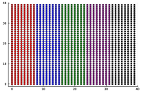
(a) Original Subgraphs

(b) $\mathcal{W}_{1}$

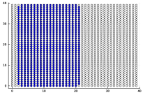
(c) $\mathcal{W}_{2}$

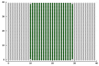
(d) $\mathcal{W}_{3}$

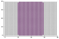
(e) $\mathcal{W}_{4}$

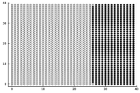
(f) $\mathcal{W}_{5}$

Figure 2: The illustration of the graph decomposition. We consider the case that the full graph is a two-dimensional graph, $[0,39]\times[0,39]$. 2(a) - 2(f) describe one way to decompose the full graph into five overlapping subgraphs. 2(a) shows the original subgraphs (Different colors represent different subgraphs). 2(b) - 2(f) show the overlapping subgraphs with the size of overlap $b=6$.

Graph decomposition The graph of Eq. 59 is a two-dimensional square graph with 40 nodes on the x-axis and 40 nodes on the y-axis. We divide the $x$-axis into 5 equal intervals and keep the $y$ axis the same. Then, five disjoint subgraphs are $[0,7]\times[0,39],\cdots,[32,39]\times[0,39]$ respectively. The illustration of the graph decomposition is in Fig. 2.
Simulation setting We use 5 size of overlaps $b=\{1,2,4,6,8\}$ and set $\eta_{1}=5$, $\eta_{2}=0.1$, $\beta_{1}=0.1$, and $\mu=1$. In order to find the step size of each iteration, we first initialize the stepsize $\alpha^{\tau}$ to be 1 and continue to decrease it by setting $\alpha^{\tau}=0.9\alpha^{\tau}$ until it satisfies Armijo condition. For the global convergence experiment, we generate 5 initial iterates randomly by $u^{0}_{k},z^{0}_{k},\lambda^{0}_{k}\overset{iid}{\sim}\text{Uniform}(-10^{2},10^{2})$. Then we apply different $b$ to solve Eq. 58 with every initialization. For local convergence, we set the initial iterate $(\boldsymbol{u}^{0},\boldsymbol{z}^{0},\boldsymbol{\lambda}^{0})=(\boldsymbol{-10},\boldsymbol{-10},\boldsymbol{0})$ in order to make it close to the local solution. The solutions of subproblems Eq. 4 are obtained by solving their KKT equations directly and the reference solutions $(\boldsymbol{x}^{*},\boldsymbol{\lambda}^{*})$ are generated by the JuMP/Julia package [12] with IPOpt solver [30].

Results summary

FOGD converged from each of the five random initial iterates converge for all five size of overlaps s seen in Fig. 3(a)-3(e), validating our global convergence claim. In Fig. 3(f), we show that the logarithm of the node-wise primal-dual error $\Psi^{\tau}$ decays linearly with respect to $\tau$, and the convergence rate increases when the size of the overlap increases. This is consistent with our local convergence result.

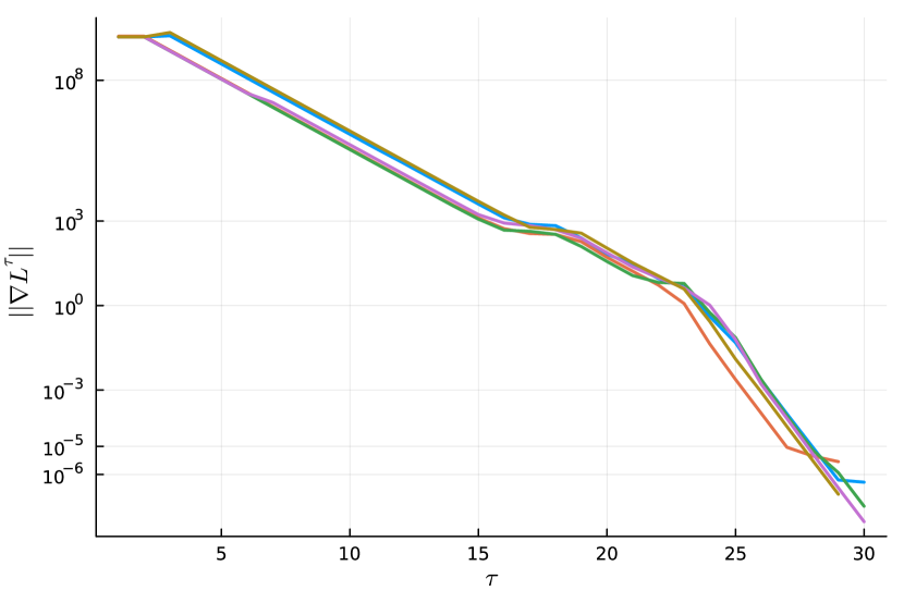
(a) $b=1$

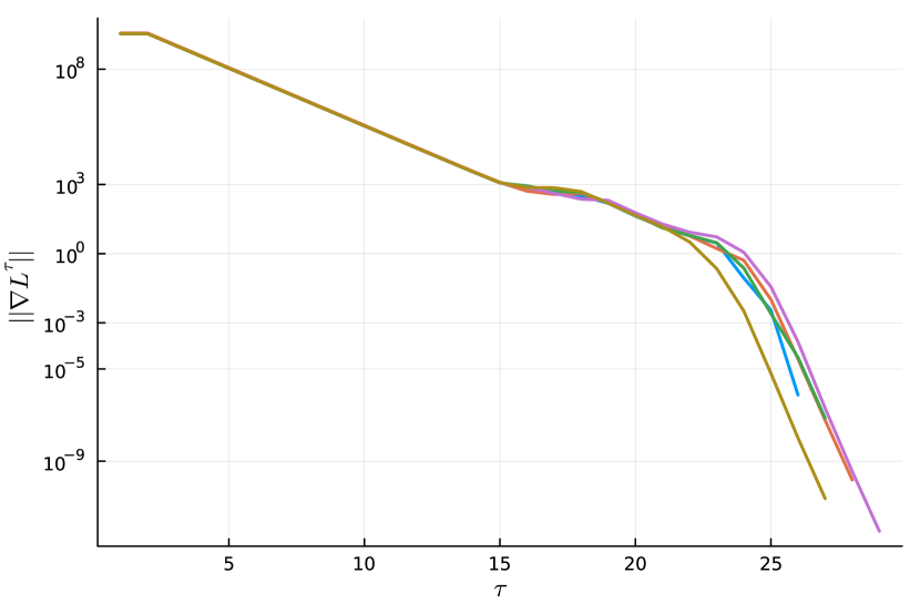
(b) $b=2$

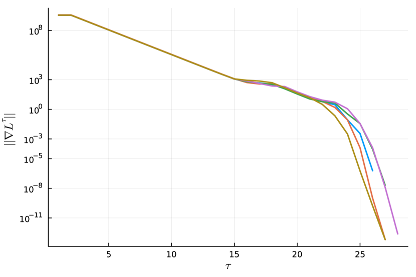
(c) $b=4$

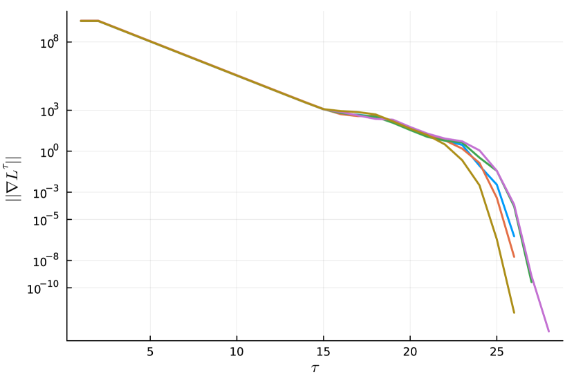
(d) $b=6$

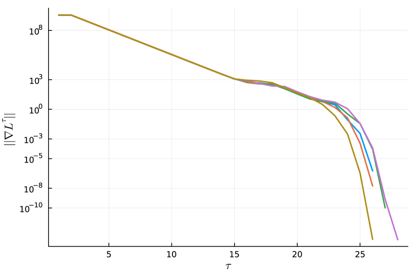
(e) $b=8$

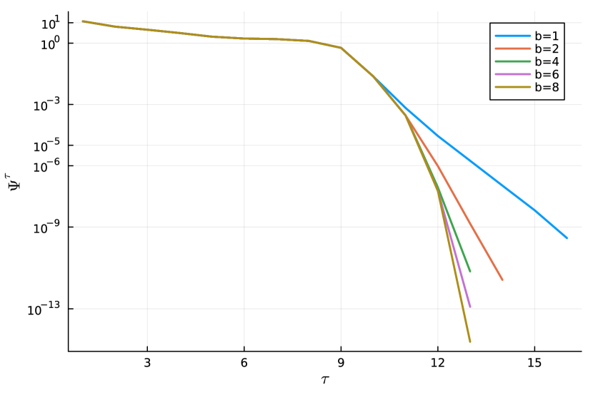
(f) local convergence

Figure 3: Global convergence and local convergence plots. The global convergence is displayed in Fig. 3(a)-3(e) where we plot the KKT residuals of each iteration. In every figure, there are five lines representing different initial conditions and they all converge. It indicates that FOGD converges for all initialization and size of overlaps. The local convergence is displayed in Fig. 3(f) and $\Psi^{\tau}$ is defined in Eq. 43. We set the initial iterate $(\boldsymbol{u}^{0},\boldsymbol{z}^{0},\boldsymbol{\lambda}^{0})=(\boldsymbol{-10},\boldsymbol{-10},\boldsymbol{0})$ and change the size of overlaps. Every line of it represents a different size of overlap. We can see $\Psi^{\tau}$ decays linearly with respect to $\tau$ and larger $b$ leads to a faster convergence rate.

7 Conclusion

This paper presents the fast overlapping graph decomposition algorithm (FOGD) for solving graph-structured general nonlinear optimization problems. We combine SQP with an exact augmented Lagrangian merit function and apply the OGD procedure to get the approximated Newton directions of SQP. We establish its global convergence in Theorem 4.5 and its local convergence in Theorem 5.5. We also reveal that the local convergence rate of FOGD improves with the increasing size of overlap. Our proposed algorithm balances the flexibility and efficiency of optimization solvers, which overcomes the main disadvantage of the common decomposition algorithms, and complements the overlapping Schwarz schemes, which lack global convergence guarantee. Numerical results of the semilinear PDEs controlled optimization problem in Section 6 verify our theoretical findings in Section 2 - Section 5. However, similar to FOTD [21], one drawback of FOGD is that it takes two steps to modify Hessian matrices and solve linear quadratic subproblems. It is better to have an algorithm to combine these two steps into one step, such as the parallel quasi-Newton scheme [9]. Further, the extension of FOGD is a promising topic, since the Schwarz schemes were demonstrated to outperform ADMM in [29], and both FOGD and the Schwarz schemes incorporate the OGD procedure to solve subproblems suggesting the close relationship among them. It is worthwhile to embed OGD into other advanced SQP frameworks and compare their performances.

Appendix A Proofs of results in Section 3

A.1 Proof of Lemma 3.1

We omit the iteration index $\tau$ for the simplicity of notation. First, we denote the Jacobian matrix of $\mathcal{L}\mathcal{P}^{\mu}_{i}$ as $G_{i}$ and we want to prove that $G_{i}$ has the full row rank. By observing the problem formulation, one can see that $G_{i}$ is a submatrix of $G$ where $G$ is the Jacobian matrix of Eq. 3. Since $G_{i}=\nabla_{\boldsymbol{\tilde{x}}_{i}}\boldsymbol{c}_{\mathcal{W}_{i}\setminus\tilde{\mathcal{W}}_{i}}$, $\boldsymbol{\tilde{x}}_{i}=\{x_{j}\}_{j\in\mathcal{W}_{i}}$, and $N_{\mathcal{G}}[\mathcal{W}_{i}\setminus\tilde{\mathcal{W}}_{i}]=\mathcal{W}_{i}$, we can obtain $\nabla_{x_{j}}\boldsymbol{c}_{k}=\boldsymbol{0},\;\forall k\in\mathcal{W}_{i}\setminus\tilde{\mathcal{W}}_{i},j\in\mathcal{V}\setminus\mathcal{W}_{i}$ and the permuted Jacobian matrix of Eq. 1 (denote it as $G_{P}$) as follows

$$G_{P}=\begin{bmatrix}G_{i}&\boldsymbol{0}\\ J&K\\ \end{bmatrix}$$

where $J$ and $K$ are nonzero matrices. Since $G_{i}(G_{i})^{T}$ is the diagonal submatrix of $G_{P}(G_{P})^{T}$, the smallest eigenvalue of $G_{i}(G_{i})^{T}$ is greater than or equal to the smallest eigenvalue of $G_{P}(G_{P})^{T}$. Since $G_{P}$ is the permutation of $G$, Assumption 11 holds for $G_{P}$ as well. Therefore, it suffices to show that there exists $\beta$ such that $G^{\tau}_{i}(G^{\tau}_{i})^{T}\succeq\beta I$.

Second, we want to show the reduced Hessian matrix of $\mathcal{L}\mathcal{P}_{i}^{\mu}$ is lower bounded by $(\gamma_{RH}/2)I$. By Assumptions 3-11 and [27, Lemma 5.6], we have $\hat{H}+\bar{\mu}(\nabla_{\boldsymbol{x}}\boldsymbol{c})^{T}\nabla_{\boldsymbol{x}}\boldsymbol{c}\succeq\frac{\gamma_{RH}}{2}I$ for any $\mu\geq\bar{\mu}$. Then, one observation is that $\hat{H}_{i}+\mu(\nabla_{\boldsymbol{\widetilde{x}}_{i}}\boldsymbol{c})^{T}\nabla_{\boldsymbol{\widetilde{x}}_{i}}\boldsymbol{c}$ is the diagonal submatrix of $\hat{H}+\bar{\mu}(\nabla_{\boldsymbol{x}}\boldsymbol{c})^{T}\nabla_{\boldsymbol{x}}\boldsymbol{c}$ which yields

(60) $$\hat{H}_{i}+\mu(\nabla_{\boldsymbol{\widetilde{x}}_{i}}\boldsymbol{c})^{T}\nabla_{\boldsymbol{\widetilde{x}}_{i}}\boldsymbol{c}\succeq\frac{\gamma_{RH}}{2}I,$$

where we denote $\hat{H}_{i}=\hat{H}[\mathcal{W}_{i}][\mathcal{W}_{i}]$. Since $\nabla_{\boldsymbol{\widetilde{x}}_{i}}\boldsymbol{c}_{\mathcal{W}_{i}\setminus\tilde{\mathcal{W}}_{i}}$ is the submatrix of $\nabla_{\boldsymbol{\widetilde{x}}_{i}}\boldsymbol{c}$, we have that $(\nabla_{\boldsymbol{\widetilde{x}}_{i}}\boldsymbol{c})^{T}\nabla_{\boldsymbol{\widetilde{x}}_{i}}\boldsymbol{c}\,Z_{i}=(\nabla_{\boldsymbol{\widetilde{x}}_{i}}\boldsymbol{c}_{\hat{\mathcal{W}_{i}}})^{T}\nabla_{\boldsymbol{\widetilde{x}}_{i}}\boldsymbol{c}_{\hat{\mathcal{W}_{i}}}\,Z_{i}$ where $Z_{i}$ is the null space of $\nabla_{\boldsymbol{\widetilde{x}}_{i}}\boldsymbol{c}_{\mathcal{W}_{i}\setminus\tilde{\mathcal{W}}_{i}}$. Then, we obtain

$$\begin{split}ReH\left(\hat{H}_{i}+\mu(\nabla_{\boldsymbol{\widetilde{x}}_{i}}\boldsymbol{c})^{T}\nabla_{\boldsymbol{\widetilde{x}}_{i}}\boldsymbol{c},\nabla_{\boldsymbol{\widetilde{x}}_{i}}\boldsymbol{c}_{\mathcal{W}_{i}\setminus\tilde{\mathcal{W}}_{i}}\right)=ReH\left(\hat{H}_{i}+\mu(\nabla_{\boldsymbol{\widetilde{x}}_{i}}\boldsymbol{c}_{\hat{\mathcal{W}_{i}}})^{T}\nabla_{\boldsymbol{\widetilde{x}}_{i}}\boldsymbol{c}_{\hat{\mathcal{W}_{i}}},\nabla_{\boldsymbol{\widetilde{x}}_{i}}\boldsymbol{c}_{\mathcal{W}_{i}\setminus\tilde{\mathcal{W}}_{i}}\right),\end{split}$$

where $ReH(H,G)=Z^{T}HZ$ is the reduced Hessian matrix and $Z$ is the null space of $G$. Given Eq. 60 and the fact that $\hat{H}_{i}+\mu(\nabla_{\boldsymbol{\widetilde{x}}_{i}}\boldsymbol{c}_{\hat{\mathcal{W}_{i}}})^{T}\nabla_{\boldsymbol{\widetilde{x}}_{i}}\boldsymbol{c}_{\hat{\mathcal{W}_{i}}}$ is the Hessian matrix of the Lagrangian function of $\mathcal{L}\mathcal{P}_{i}^{\mu}$, we can conclude that there exists $\gamma_{RH}$ such that

$$ReH\left(\hat{H}_{i}+\mu(\nabla_{\boldsymbol{\widetilde{x}}_{i}}\boldsymbol{c}_{\hat{\mathcal{W}_{i}}})^{T}\nabla_{\boldsymbol{\widetilde{x}}_{i}}\boldsymbol{c}_{\hat{\mathcal{W}_{i}}},\nabla_{\boldsymbol{\widetilde{x}}_{i}}\boldsymbol{c}_{\mathcal{W}_{i}\setminus\tilde{\mathcal{W}}_{i}}\right)\succeq\frac{\gamma_{RH}}{2}I.$$

Since $\boldsymbol{d}_{i}$ only affects linear terms, the reduced Hessian $\mathcal{L}\mathcal{P}^{\mu}_{i}$ is independent of $\boldsymbol{d}_{i}$. We proved that the reduced Hessian of $\mathcal{L}\mathcal{P}_{i}^{\mu}(\boldsymbol{d}_{i})$ is positive definite for any $\boldsymbol{d}_{i}$ and the proof is complete.

Appendix B Proofs of results in Section 4

B.1 Proof of Lemma 4.1

First, we want to prove Eq. 27. By Assumptions 3, 4 and [27, Lemma 5.10], there exists a constant $\gamma_{u}=e(1)L_{\text{cpt}}$ such that

$$\|H(\boldsymbol{x},\boldsymbol{\lambda})\|\leq\gamma_{u},\quad\|\nabla_{q,q}\tilde{\mathcal{L}}(\boldsymbol{x},\boldsymbol{\lambda})\|\leq\gamma_{u},\quad\text{for $\forall\,\boldsymbol{x}\in\mathcal{X},\,\boldsymbol{\lambda}\in\Lambda$},$$

Since $\hat{H}(\boldsymbol{x},\boldsymbol{\lambda})$ and $G(\boldsymbol{x},\boldsymbol{\lambda})$ are submatrices of $\nabla_{q,q}\tilde{\mathcal{L}}(\boldsymbol{x},\boldsymbol{\lambda})$, and $G_{i}(\boldsymbol{x})$ is a submatrix of $G(\boldsymbol{x})$, we complete the proof of Eq. 27.

Next, we want to prove Eq. 28. Its proof is similar to the proof of Lemma 5.1 in [21] and we give the full proof because of the subtle differences in settings. Observing that $G^{T}(GG^{T})^{-1}G+ZZ^{T}=I$ where $Z$ is the span of $\{w:Gw=0\}$, we can verify that

$$\begin{split}\mathcal{B}&=\begin{pmatrix}\hat{H}&G^{T}\\ G&\boldsymbol{0}\\ \end{pmatrix}^{-1}=\begin{pmatrix}\mathcal{B}_{1}&\mathcal{B}_{2}^{T}\\ \mathcal{B}_{2}&\mathcal{B}_{3}\\ \end{pmatrix}\\ \mathcal{B}_{1}&=Z(Z^{T}\hat{H}Z)^{-1}Z^{T},\quad\mathcal{B}_{2}=(GG^{T})^{-1}G(I-\hat{H}Z(Z^{T}\hat{H}Z)^{-1}Z^{T}),\\ \mathcal{B}_{3}&=(GG^{T})^{-1}G(\hat{H}Z(Z^{T}\hat{H}Z)^{-1}Z^{T}\hat{H}-\hat{H})G^{T}(GG^{T})^{-1}\end{split}$$

Finally, by Assumptions 3-11 and Lemma 3.1, we have $\|\mathcal{B}_{1}\|\leq\frac{1}{\gamma_{RH}}$, $\|\mathcal{B}_{2}\|\leq\|(GG^{T})^{-1}G\|$ $\times\left(1+\frac{\gamma_{u}}{\gamma_{RH}}\right)\leq\frac{1}{\sqrt{\beta}}\left(1+\frac{\gamma_{u}}{\gamma_{RH}}\right)$, and $\|\mathcal{B}_{3}\|\leq\frac{1}{\beta}\left(\gamma_{u}+\frac{\gamma_{u}^{2}}{\gamma_{RH}}\right)$. Since $\|\mathcal{B}\|\leq\|\mathcal{B}_{1}\|+2\|\mathcal{B}_{2}\|+\|\mathcal{B}_{3}\|$, we complete the proof.

Appendix C Proofs of results in Section 5

C.1 Proof of Lemma 5.1

By Eq. 8, we only need to show for sufficiently large $\tau$

(61) $$\mathcal{L}_{\eta}(\boldsymbol{x}^{\tau}+\tilde{\Delta}\boldsymbol{x}^{\tau},\boldsymbol{\lambda}^{\tau}+\tilde{\Delta}\boldsymbol{\lambda}^{\tau})\leq\mathcal{L}_{\eta}(\boldsymbol{x}^{\tau},\boldsymbol{\lambda}^{\tau})+\beta_{1}\begin{pmatrix}\nabla_{\boldsymbol{x}}\mathcal{L}_{\eta}^{\tau}\\ \nabla_{\boldsymbol{\lambda}}\mathcal{L}_{\eta}^{\tau}\\ \end{pmatrix}^{T}\begin{pmatrix}\tilde{\Delta}\boldsymbol{x}^{\tau}\\ \tilde{\Delta}\boldsymbol{\lambda}^{\tau}\\ \end{pmatrix}.$$

Since objective functions and constraints are twice continuous and differentiable, $\nabla^{2}\mathcal{L}_{\eta}$ is continuous so that we can apply Taylor expansion to $\mathcal{L}_{\eta}(\boldsymbol{x}^{\tau}+\tilde{\Delta}\boldsymbol{x}^{\tau},\boldsymbol{\lambda}^{\tau}+\tilde{\Delta}\boldsymbol{\lambda}^{\tau})$ as follows

(62) $$\begin{split}\mathcal{L}_{\eta}(\boldsymbol{x}^{\tau}+\tilde{\Delta}\boldsymbol{x}^{\tau},\boldsymbol{\lambda}^{\tau}+\tilde{\Delta}\boldsymbol{\lambda}^{\tau})&\leq\mathcal{L}_{\eta}(\boldsymbol{x}^{\tau},\boldsymbol{\lambda}^{\tau})+\begin{pmatrix}\nabla_{\boldsymbol{x}}\mathcal{L}_{\eta}^{\tau}\\ \nabla_{\boldsymbol{\lambda}}\mathcal{L}_{\eta}^{\tau}\\ \end{pmatrix}^{T}\begin{pmatrix}\tilde{\Delta}\boldsymbol{x}^{\tau}\\ \tilde{\Delta}\boldsymbol{\lambda}^{\tau}\\ \end{pmatrix}\\ &+\frac{1}{2}\begin{pmatrix}\tilde{\Delta}\boldsymbol{x}^{\tau}\\ \tilde{\Delta}\boldsymbol{\lambda}^{\tau}\\ \end{pmatrix}^{T}\nabla^{2}\mathcal{L}_{\eta}^{\tau}\begin{pmatrix}\tilde{\Delta}\boldsymbol{x}^{\tau}\\ \tilde{\Delta}\boldsymbol{\lambda}^{\tau}\\ \end{pmatrix}+o(\|(\tilde{\Delta}\boldsymbol{x}^{\tau},\tilde{\Delta}\boldsymbol{\lambda}^{\tau})\|^{2}).\end{split}$$

where

$$\begin{split}\nabla_{\boldsymbol{x}}^{2}\mathcal{L}_{\eta}&=H+\eta_{1}G^{T}G+\eta_{2}H^{2}+\eta_{1}\langle\nabla_{\boldsymbol{x}}G,\boldsymbol{c}\rangle+\eta_{2}\langle\nabla_{\boldsymbol{x}}H,\nabla_{\boldsymbol{x}}\mathcal{L}\rangle,\\ \nabla_{\boldsymbol{x},\boldsymbol{\lambda}}\mathcal{L}_{\eta}&=G^{T}+\eta_{2}HG^{T}+\eta_{2}\langle\nabla_{\boldsymbol{\lambda}}H,\nabla_{\boldsymbol{x}}\mathcal{L}\rangle,\quad\nabla_{\boldsymbol{\lambda}}^{2}\mathcal{L}_{\eta}=\eta_{2}GG^{T}.\end{split}$$

The operator $\langle\cdot\rangle$ is defined as $\langle a(x),b\rangle:=\nabla^{T}(a^{T}(x)b)=\sum_{j=1}^{m_{1}}b_{j}\nabla^{T}a_{j}(x)\in\mathbb{R}^{m_{2}\times n}$ with $a(x):\mathbb{R}^{n}\rightarrow\mathbb{R}^{m_{1}\times m_{2}}$, $a^{T}(x)=(a_{1}(x),\cdots,a_{m_{1}}(x))$, and $b\in\mathbb{R}^{m_{1}}$. We let

$$\mathcal{H}^{\tau}:=\begin{pmatrix}H^{\tau}+\eta_{1}(G^{\tau})^{T}G^{\tau}+\eta_{2}(H^{\tau})^{2}&(I+\eta_{2}H^{\tau})(G^{\tau})^{T}\\ G^{\tau}(I+\eta_{2}H^{\tau})&\eta_{2}G^{\tau}(G^{\tau})^{T}\end{pmatrix},$$

Since the iterates converge globally, $\|\nabla\mathcal{L}^{\tau}\|=\|(\nabla_{\boldsymbol{x}}\mathcal{L}^{\tau},\boldsymbol{c}^{\tau})\|\rightarrow 0$. We apply this result to $\nabla^{2}\mathcal{L}_{\eta}^{\tau}$ and obtain

(63) $$\|\nabla^{2}\mathcal{L}_{\eta}^{\tau}-\mathcal{H}^{\tau}\|\rightarrow 0$$

Substituting Eq. 63 into Eq. 62 and combining Eq. 61 and Eq. 62, the goal of this proof is equivalent to showing

(64) $$(1-\beta_{1})\begin{pmatrix}\nabla_{\boldsymbol{x}}\mathcal{L}_{\eta}^{\tau}\\ \nabla_{\boldsymbol{\lambda}}\mathcal{L}_{\eta}^{\tau}\\ \end{pmatrix}^{T}\begin{pmatrix}\tilde{\Delta}\boldsymbol{x}^{\tau}\\ \tilde{\Delta}\boldsymbol{\lambda}^{\tau}\\ \end{pmatrix}+\frac{1}{2}\begin{pmatrix}\tilde{\Delta}\boldsymbol{x}^{\tau}\\ \tilde{\Delta}\boldsymbol{\lambda}^{\tau}\\ \end{pmatrix}^{T}\mathcal{H}^{\tau}\begin{pmatrix}\tilde{\Delta}\boldsymbol{x}^{\tau}\\ \tilde{\Delta}\boldsymbol{\lambda}^{\tau}\\ \end{pmatrix}+o(\|(\tilde{\Delta}\boldsymbol{x}^{\tau},\tilde{\Delta}\boldsymbol{\lambda}^{\tau})\|^{2})\leq 0.$$

One observation is

$$\begin{split}&\quad\begin{pmatrix}\nabla_{\boldsymbol{x}}\mathcal{L}_{\eta}^{\tau}\\ \nabla_{\boldsymbol{\lambda}}\mathcal{L}_{\eta}^{\tau}\\ \end{pmatrix}^{T}\begin{pmatrix}\tilde{\Delta}\boldsymbol{x}^{\tau}\\ \tilde{\Delta}\boldsymbol{\lambda}^{\tau}\\ \end{pmatrix}+\begin{pmatrix}\tilde{\Delta}\boldsymbol{x}^{\tau}\\ \tilde{\Delta}\boldsymbol{\lambda}^{\tau}\\ \end{pmatrix}^{T}\mathcal{H}^{\tau}\begin{pmatrix}\tilde{\Delta}\boldsymbol{x}^{\tau}\\ \tilde{\Delta}\boldsymbol{\lambda}^{\tau}\\ \end{pmatrix}\\ &\overset{\begin{subarray}{c}\lx@cref{creftype~refnum}{eq31}\\ \lx@cref{creftype~refnum}{eq35}\end{subarray}}{=}\begin{pmatrix}\tilde{\Delta}\boldsymbol{x}^{\tau}\\ \tilde{\Delta}\boldsymbol{\lambda}^{\tau}\\ \end{pmatrix}^{T}\left\{\mathcal{H}^{\tau}-\begin{pmatrix}\hat{H}^{\tau}+\eta_{1}(G^{\tau})^{T}G^{\tau}+\eta_{2}H^{\tau}\hat{H}^{\tau}&(I+\eta_{2}H^{\tau})(G^{\tau})^{T}\\ G^{\tau}(I+\eta_{2}\hat{H}^{\tau})&\eta_{2}G^{\tau}(G^{\tau})^{T}\end{pmatrix}\right\}\begin{pmatrix}\Delta\boldsymbol{x}^{\tau}\\ \Delta\boldsymbol{\lambda}^{\tau}\\ \end{pmatrix}\\ &\quad+\begin{pmatrix}\tilde{\Delta}\boldsymbol{x}^{\tau}\\ \tilde{\Delta}\boldsymbol{\lambda}^{\tau}\\ \end{pmatrix}^{T}\mathcal{H}^{\tau}\begin{pmatrix}\tilde{\Delta}\boldsymbol{x}^{\tau}-\Delta\boldsymbol{x}^{\tau}\\ \tilde{\Delta}\boldsymbol{\lambda}^{\tau}-\Delta\boldsymbol{\lambda}^{\tau}\\ \end{pmatrix}=:\mathcal{I}_{3}+\mathcal{I}_{4}\end{split}$$

For term $\mathcal{I}_{3}$, denote $\Delta H^{\tau}=H^{\tau}-\hat{H}^{\tau}$

(65) $$\begin{split}\mathcal{I}_{3}&=\begin{pmatrix}\tilde{\Delta}\boldsymbol{x}^{\tau}\\ \tilde{\Delta}\boldsymbol{\lambda}^{\tau}\\ \end{pmatrix}^{T}\begin{pmatrix}(I+\eta_{2}H^{\tau})\Delta H^{\tau}&\boldsymbol{0}\\ \eta_{2}G^{\tau}\Delta H^{\tau}&\boldsymbol{0}\end{pmatrix}\begin{pmatrix}\Delta\boldsymbol{x}^{\tau}\\ \Delta\boldsymbol{\lambda}^{\tau}\\ \end{pmatrix}\overset{\lx@cref{creftype~refnum}{eq53}}{\leq}\|(\tilde{\Delta}\boldsymbol{x}^{\tau},\tilde{\Delta}\boldsymbol{\lambda}^{\tau})\|\cdot(1+2\eta_{2}\gamma)\|\Delta H^{\tau}\Delta\boldsymbol{x}^{\tau}\|\\ &\leq 2(1+2\eta_{2}\gamma)\|(\Delta\boldsymbol{x}^{\tau},\Delta\boldsymbol{\lambda}^{\tau})\|o(\|\Delta\boldsymbol{x}^{\tau}\|)=o(\|(\Delta\boldsymbol{x}^{\tau},\Delta\boldsymbol{\lambda}^{\tau})\|^{2})\end{split}$$

where the last inequality holds because of Eq. 25 and Assumption 5. For term $\mathcal{I}_{4}$, we have

(66) $$\begin{split}\mathcal{I}_{4}&\leq\|(\tilde{\Delta}\boldsymbol{x}^{\tau},\tilde{\Delta}\boldsymbol{\lambda}^{\tau})\|\|\mathcal{H}^{\tau}\|\|(\tilde{\Delta}\boldsymbol{x}^{\tau}-\Delta\boldsymbol{x}^{\tau},\tilde{\Delta}\boldsymbol{\lambda}^{\tau}-\Delta\boldsymbol{\lambda}^{\tau})\|\\ &\overset{\begin{subarray}{c}\lx@cref{creftype~refnum}{eq51}\\ \lx@cref{creftype~refnum}{eq53}\end{subarray}}{\leq}2\delta\|(\Delta\boldsymbol{x}^{\tau},\Delta\boldsymbol{\lambda}^{\tau})\|^{2}\gamma\{3+\gamma(4\eta_{2}+\eta_{1})\}\end{split}$$

Then, we obtain

$$\begin{split}&(1-\beta_{1})\begin{pmatrix}\nabla_{\boldsymbol{x}}\mathcal{L}_{\eta}^{\tau}\\ \nabla_{\boldsymbol{\lambda}}\mathcal{L}_{\eta}^{\tau}\\ \end{pmatrix}^{T}\begin{pmatrix}\tilde{\Delta}\boldsymbol{x}^{\tau}\\ \tilde{\Delta}\boldsymbol{\lambda}^{\tau}\\ \end{pmatrix}+\frac{1}{2}\begin{pmatrix}\tilde{\Delta}\boldsymbol{x}^{\tau}\\ \tilde{\Delta}\boldsymbol{\lambda}^{\tau}\\ \end{pmatrix}^{T}\mathcal{H}^{\tau}\begin{pmatrix}\tilde{\Delta}\boldsymbol{x}^{\tau}\\ \tilde{\Delta}\boldsymbol{\lambda}^{\tau}\\ \end{pmatrix}+o(\|(\tilde{\Delta}\boldsymbol{x}^{\tau},\tilde{\Delta}\boldsymbol{\lambda}^{\tau})\|^{2})\\ &=\left(\frac{1}{2}-\beta_{1}\right)\begin{pmatrix}\nabla_{\boldsymbol{x}}\mathcal{L}_{\eta}^{\tau}\\ \nabla_{\boldsymbol{\lambda}}\mathcal{L}_{\eta}^{\tau}\\ \end{pmatrix}^{T}\begin{pmatrix}\tilde{\Delta}\boldsymbol{x}^{\tau}\\ \tilde{\Delta}\boldsymbol{\lambda}^{\tau}\\ \end{pmatrix}+\frac{1}{2}\mathcal{I}_{3}+\frac{1}{2}\mathcal{I}_{4}+o(\|(\tilde{\Delta}\boldsymbol{x}^{\tau},\tilde{\Delta}\boldsymbol{\lambda}^{\tau})\|^{2})\\ &\leq(\frac{1}{2}-\beta_{1})\begin{pmatrix}\nabla_{\boldsymbol{x}}\mathcal{L}_{\eta}^{\tau}\\ \nabla_{\boldsymbol{\lambda}}\mathcal{L}_{\eta}^{\tau}\\ \end{pmatrix}^{T}\begin{pmatrix}\tilde{\Delta}\boldsymbol{x}^{\tau}\\ \tilde{\Delta}\boldsymbol{\lambda}^{\tau}\\ \end{pmatrix}+\delta\|(\Delta\boldsymbol{x}^{\tau},\Delta\boldsymbol{\lambda}^{\tau})\|^{2}\gamma\{3+\gamma(4\eta_{2}+\eta_{1})\}+o(\|(\Delta\boldsymbol{x}^{\tau},\Delta\boldsymbol{\lambda}^{\tau})\|^{2})\\ &\leq-\left(\left(\frac{1}{2}-\beta_{1}\right)\left(\frac{\eta_{2}\beta}{8}-\delta\{3\gamma+4\eta_{2}\gamma^{2}+\eta_{1}\gamma^{2}\}\right)-\gamma\{3+\gamma(4\eta_{2}+\eta_{1})\}\delta\right)\|(\Delta\boldsymbol{x}^{\tau},\Delta\boldsymbol{\lambda}^{\tau})\|^{2}\\ &+o(\|(\Delta\boldsymbol{x}^{\tau},\Delta\boldsymbol{\lambda}^{\tau})\|^{2})\end{split}$$

where the first inequality holds because of Eq. 65 and Eq. 66, and the second inequality holds because of Eq. 37. Since $\delta\leq\frac{\frac{1}{2}-\beta_{1}}{\frac{3}{2}-\beta_{1}}\frac{\eta_{2}\beta}{8(3\gamma+4\eta_{2}\gamma^{2}+\eta_{1}\gamma^{2})}$, the coefficient of $\|(\Delta\boldsymbol{x}^{\tau},\Delta\boldsymbol{\lambda}^{\tau})\|^{2}$ is negative and it completes the proof.

Government License: The submitted manuscript has been created by UChicago Argonne, LLC, Operator of Argonne National Laboratory (“Argonne”). Argonne, a U.S. Department of Energy Office of Science laboratory, is operated under Contract No. DE-AC02-06CH11357. The U.S. Government retains for itself, and others acting on its behalf, a paid-up nonexclusive, irrevocable worldwide license in said article to reproduce, prepare derivative works, distribute copies to the public, and perform publicly and display publicly, by or on behalf of the Government. The Department of Energy will provide public access to these results of federally sponsored research in accordance with the DOE Public Access Plan. http://energy.gov/downloads/doe-public-access-plan.

References

• [1] H. Antil, D. P. Kouri, and D. Ridzal, ALESQP: An augmented lagrangian equality-constrained SQP method for optimization with general constraints, SIAM Journal on Optimization, 33 (2023), pp. 237–266.
• [2] A. Beccuti, T. Geyer, and M. Morari, Temporal lagrangian decomposition of model predictive control for hybrid systems, in 2004 43rd IEEE Conference on Decision and Control (CDC) (IEEE Cat. No.04CH37601), IEEE, 2004.
• [3] D. P. Bertsekas, Constrained optimization and Lagrange multiplier methods, Academic press, 2014.
• [4] J. T. Betts, Practical Methods for Optimal Control and Estimation Using Nonlinear Programming, Society for Industrial and Applied Mathematics, jan 2010.
• [5] L. T. Biegler, Nonlinear Programming, Society for Industrial and Applied Mathematics, jan 2010.
• [6] L. T. Biegler, O. Ghattas, M. Heinkenschloss, and B. van Bloemen Waanders, Large-Scale PDE-Constrained Optimization: An Introduction, Springer Berlin Heidelberg, 2003.
• [7] P. T. Boggs and J. W. Tolle, Sequential quadratic programming, Acta numerica, 4 (1995), pp. 1–51.
• [8] R. H. Byrd, F. E. Curtis, and J. Nocedal, An inexact SQP method for equality constrained optimization, SIAM Journal on Optimization, 19 (2008), pp. 351–369.
• [9] R. H. Byrd, R. B. Schnabel, and G. A. Shultz, Parallel quasi-newton methods for unconstrained optimization, Mathematical Programming, 42 (1988), pp. 273–306.
• [10] T. F. Chan and B. F. Smith, Domain decomposition and multigrid algorithms for elliptic problems on unstructured meshes, Contemporary Mathematics, 180 (1994), pp. 175–175.
• [11] T. F. Chan and J. Zou, Additive schwarz domain decomposition methods for elliptic problems on unstructured meshes, Numerical Algorithms, 8 (1994), pp. 329–346.
• [12] I. Dunning, J. Huchette, and M. Lubin, JuMP: A modeling language for mathematical optimization, SIAM Review, 59 (2017), pp. 295–320.
• [13] E. Ghadimi, A. Teixeira, I. Shames, and M. Johansson, Optimal parameter selection for the alternating direction method of multipliers (ADMM): Quadratic problems, IEEE Transactions on Automatic Control, 60 (2015), pp. 644–658.
• [14] N. I. M. Gould and P. L. Toint, SQP methods for large-scale nonlinear programming, in System Modelling and Optimization, Springer US, 2000, pp. 149–178.
• [15] J. R. Jackson and I. E. Grossmann, Temporal decomposition scheme for nonlinear multisite production planning and distribution models, Industrial & Engineering Chemistry Research, 42 (2003), pp. 3045–3055.
• [16] A. Kozma, C. Conte, and M. Diehl, Benchmarking large-scale distributed convex quadratic programming algorithms, Optimization Methods and Software, 30 (2014), pp. 191–214.
• [17] J. H. Lee, Y. M. Jung, Y. xiang Yuan, and S. Yun, A subspace SQP method for equality constrained optimization, Computational Optimization and Applications, 74 (2019), pp. 177–194.
• [18] J. M. Mulvey and B. Shetty, Financial planning via multi-stage stochastic optimization, Computers & Operations Research, 31 (2004), pp. 1–20.
• [19] S. Na, Global convergence of online optimization for nonlinear model predictive control, Advances in Neural Information Processing Systems, 34 (2021), pp. 12441–12453, https://proceedings.neurips.cc/paper/2021/hash/67d16d00201083a2b118dd5128dd6f59-Abstract.html.
• [20] S. Na and M. Anitescu, Superconvergence of online optimization for model predictive control, IEEE Transactions on Automatic Control, 68 (2023), pp. 1383–1398.
• [21] S. Na, M. Anitescu, and M. Kolar, A fast temporal decomposition procedure for long-horizon nonlinear dynamic programming, arXiv preprint arXiv:2107.11560, (2021).
• [22] S. Na, S. Shin, M. Anitescu, and V. M. Zavala, On the convergence of overlapping schwarz decomposition for nonlinear optimal control, IEEE Transactions on Automatic Control, 67 (2022), pp. 5996–6011.
• [23] J. Nocedal and S. J. Wright, Quadratic programming, Numerical optimization, (2006), pp. 448–492.
• [24] M. V. F. Pereira and L. M. V. G. Pinto, Multi-stage stochastic optimization applied to energy planning, Mathematical Programming, 52 (1991), pp. 359–375.
• [25] S. Shin, Graph-Structured Nonlinear Programming: Properties and Algorithms, The University of Wisconsin-Madison, 2021.
• [26] S. Shin, M. Anitescu, and V. M. Zavala, Overlapping schwarz decomposition for constrained quadratic programs, in 2020 59th IEEE Conference on Decision and Control (CDC), IEEE, dec 2020.
• [27] S. Shin, M. Anitescu, and V. M. Zavala, Exponential decay of sensitivity in graph-structured nonlinear programs, SIAM Journal on Optimization, 32 (2022), pp. 1156–1183.
• [28] S. Shin, Y. Lin, G. Qu, A. Wierman, and M. Anitescu, Near-optimal distributed linear-quadratic regulator for networked systems, SIAM Journal on Control and Optimization, 61 (2023), pp. 1113–1135.
• [29] S. Shin, V. M. Zavala, and M. Anitescu, Decentralized schemes with overlap for solving graph-structured optimization problems, IEEE Transactions on Control of Network Systems, 7 (2020), pp. 1225–1236.
• [30] A. Wächter and L. T. Biegler, On the implementation of an interior-point filter line-search algorithm for large-scale nonlinear programming, Mathematical Programming, 106 (2005), pp. 25–57.
• [31] W. Xu and M. Anitescu, Exponentially accurate temporal decomposition for long-horizon linear-quadratic dynamic optimization, SIAM Journal on Optimization, 28 (2018), pp. 2541–2573.
• [32] V. M. Zavala, New architectures for hierarchical predictive control, IFAC-PapersOnLine, 49 (2016), pp. 43–48.
• [33] A. Zlotnik, M. Chertkov, and S. Backhaus, Optimal control of transient flow in natural gas networks, in 2015 54th IEEE Conference on Decision and Control (CDC), IEEE, dec 2015.