Time series generation for option pricing on quantum computers using tensor network
Abstract
Finance, especially option pricing, is a promising industrial field that might benefit from quantum computing. While quantum algorithms for option pricing have been proposed, it is desired to devise more efficient implementations of costly operations in the algorithms, one of which is preparing a quantum state that encodes a probability distribution of the underlying asset price. In particular, in pricing a path-dependent option, we need to generate a state encoding a joint distribution of the underlying asset price at multiple time points, which is more demanding. To address these issues, we propose a novel approach using Matrix Product State (MPS) as a generative model for time series generation. To validate our approach, taking the Heston model as a target, we conduct numerical experiments to generate time series in the model. Our findings demonstrate the capability of the MPS model to generate paths in the Heston model, highlighting its potential for path-dependent option pricing on quantum computers.
1 Introduction
Quantum computing has recently received growing attention in industries as it is expected to achieve significant speed-up for many computational problems. One of the fields people expect to benefit from quantum computers is finance, where several potential applications have already been considered, including portfolio optimization, risk management, and option pricing. See [1, 2, 3, 4, 5] for comprehensive reviews of these topics. The application we would like to address in this paper is option pricing with the Monte Carlo method, which is theoretically shown in [6] that it can achieve quadratic speed up compared with the classical counterpart. An option, a type of derivatives, is a financial contract in which the option buyer receives an amount of money (payoff) linked to an underlying asset, such as a stock, an interest rate index, a foreign exchange rate, and so on. Apart from underlying asset markets, options offer investors alternative opportunities for profits and hedging various risks. Based on the various needs of investors, a wide variety of options have been introduced. Therefore, it is a central problem for financial institutions to price options in a suitable manner in order to trade and manage them.
Following the quantum algorithm for Monte Carlo integration (QMCI) in [6], which is based on Quantum Amplitude Estimation (QAE) [7], quantum approaches for Monte Carlo-based option pricing have been proposed [8, 9, 10]. The option price is expressed as the expectation of the payoff in a stochastic model of the time evolution of the underlying asset price, and thus its evaluation can be sped up by QMCI. Although these sound promising, it is unclear whether it be practicable on real quantum devices, as among the procedures are costly operations such as preparing quantum states that encode probability distributions of the underlying asset price in the amplitude. Using the famous Grover-Rudolph method [11], it is possible to generate such a state if we can express a cumulative distribution in a given interval by a simple formula [10]. However, this approach requires many runs of quantum circuits for arithmetic operations [12], which results in large gate costs. Moreover, the task becomes more demanding, if we would like to price not only European-type options, in which the payoff depends on the underlying asset price on a single date, but also path-dependent ones, whose payoff depends on the asset price at multiple dates. That is, we need to generate a quantum state that encodes the joint distribution of the asset price at the different time points. In other words, we need to prepare a state encoding the distribution of time series, or paths, of the asset price.
To reduce the cost of state preparation, some alternative methods using no arithmetic circuit have been proposed. Along with methods with rigorous error bounds [13, 14, 15, 16, 17, 18, 19, 20], there are some heuristic methods, which might be able to reduce the cost further [21, 22, 23, 24, 19]. In particular, some of such methods use quantum generative modeling. [21] proposed the quantum generative adversarial networks (GAN), claiming it can reduce the number of quantum gates for loading probability distributions. The successive work [25] generalized the framework of quantum GAN, along with the improvement of classical GAN. However, as far as the authors know, there is no previous study on preparing a state encoding the time series distribution via generative modeling in the context of option pricing on a quantum computer. That is what we would like to address in this paper.
To Tackle this problem, we make good use of Matrix Product State (MPS) as a generative model. MPS, a kind of Tensor Network (TN), which was originally developed to represent quantum many-body wave functions efficiently on classical computers, is a powerful and flexible tool to approximate higher-order tensors as the network of lower-order tensors, thereby reducing the complexity of original tensors. This capability has led to recent applications of MPS in machine learning [26, 27, 28], which includes the particular focus on generative modeling [29, 30, 31]. We aim to utilize the MPS-based generative modeling for time series. Although generative modeling via MPS is classically tractable, it is strongly related to quantum computing since, given an MPS, we can generate the state on qubits with the corresponding wave function by a quantum circuit in an efficient manner [32, 33, 34]. In fact, there are some studies on MPS-based methods for function-encoding quantum state preparation [22, 24], although they are not on a time series distribution. Then, we conceive the following approach for option pricing on a quantum computer with the aid of MPS: we can find the MPS that generates asset price paths in a given model by a classical computer, and then use the corresponding state generation circuit in QMCI.
That being said, in this paper, we investigate the MPS model for generating time series with the goal of pricing options in finance. As an illustration of our methodology, we focus on the Heston model [35], a well-known and widely used stochastic process in the financial industry. To validate our approach, we generate price paths using the MPS model and compute prices of path-dependent options through classical Monte Carlo simulations. We find that the MPS model can successfully generate the price paths of the Heston model and be used in pricing these options.
The remainder of this paper is organized as follows. In Section 2, we review the basics of option pricing and introduce the Heston model. We also briefly comment on the framework of the quantum algorithm for option pricing. Section 3 is devoted to proposing MPS for generative modeling of time series. In Section 4, we report the validity of the proposed MPS model in option pricing by conducting numerical experiments. Finally, Section 5 concludes this paper with a summary and outlook.
2 Financial background
In this section, we aim to provide a review of option pricing with a particular focus on the Monte Carlo method. First, we will outline the concept of options, and explain how to price them. Since we consider the Heston model in this paper, we briefly introduce that model. Finally, we comment on option pricing with a quantum computer.
2.1 Option pricing
An option is originally a financial contract between two parties, one of which, the option holder, possesses the right, but not the obligation, to either buy or sell an underlying asset at a pre-determined price (strike), on a future date. If the holder has a right to buy (resp. sell) the underlying asset, the option is referred to as a call (resp. put) option. Let be an asset price at time and consider a call option written on that asset exercisable on a maturity date . At the maturity date, the holder exercises a right to buy the asset if its price is higher than the strike . This is equivalent to getting a profit , since the asset is worth . Conversely, if , the holder chooses not to exercise the right and receives nothing. In total, this option is equivalent to the contract in which the option holder receives the payoff
| (1) |
at .
Derived from this kind of option called a European option, many kinds of options with various payoffs have been developed. In particular, our study focuses on path-dependent options, whose payoff depends not on the asset price at a single time point but on the values at multiple time points or the entire path of the asset price. In the following, we present examples of such options considered in this work.
Asian option
An Asian option has a payoff depending on the average price of the underlying asset. Explicitly, a payoff of an Asian call option with a strike is given by
| (2) |
Lookback option
A lookback option has a payoff depending on the maximum or minimum price of the underlying asset over the life of the option. A payoff of a Lookback call option with a strike is given by
| (3) |
Barrier option
A barrier option has a payoff which depends on whether an underlying asset price touches the barrier level before the maturity date. While there are various types of barrier options, we consider an up-and-out barrier call option with a strike , whose payoff is given by
| (4) |
That means that the up-and-out call option expires worthless when crosses the barrier level .
In order to trade these financial products in the market, it is essential to determine their theoretical fair prices. The price of an option at the present time is given by the expectation value (see textbooks [36, 37, 38] for the details),
| (5) |
in the risk-neutral measure. Note that, for the sake of simplicity, we assume the risk-free rate to be 0 here and hereafter.
As such, the central problem in option pricing has revolved around the calculation of the above expectation value in a stochastic model of . The celebrated Black-Scholes (BS) model [39, 40] assumes that, in the risk-neutral measure, the dynamics of is given by the following stochastic differential equation (SDE)
| (6) |
where denotes a Wiener process and the volatility is a positive constant. This leads to an analytic formula for a European option price: e.g., the price of a European call with strike and maturity is
| (7) | ||||
| (8) | ||||
| (9) |
where is the cumulative distribution function of the standard normal distribution. On the other hand, when dealing with more complicated options such as the aforementioned ones, and with the underlying asset price dynamics given by a more general SDE like
| (10) |
where the volatility is some stochastic process, we need to consult numerical techniques.
Among them, we hereafter focus on the Monte Carlo method. This requires generating numerous price paths for the underlying asset based on the assumed model like Eq.(10). In reality, we cannot generate paths for continuous time but discretized paths consisting of a finite number of time points . Following the generation of simulated price paths , where is the index of the sample paths, the price of the option in Eq. (5) is estimated by
| (11) |
where the payoff function is somehow approximated if it is defined with a path on continuous time. This approach allows us to numerically evaluate complex options with path dependence. However, it should be noted that the Monte Carlo method can be computationally intensive particularly when generating a large number of paths is required: for accuracy in , the number of paths scales as . This motivates us to consider applying QMCI, which provides the speed-up as described later.
2.2 Heston model
The Heston model [35] is a popular mathematical model to describe the dynamics of the asset price and its volatility and has become widely used in the financial industry. It is one of stochastic volatility (SV) models, meaning it incorporates a stochastic process of the volatility as well as the asset price. SV models can be used when market prices of European options written on the asset do not match the prices given by the BS model, which is an often observed phenomenon called the volatility smile [41].
In the Heston model, the dynamics of the asset is given by the following SDE in the risk-neutral measure:
| (12) | ||||
| (13) |
where and are one-dimensional Wiener process with correlation , which appears as , and are positive constants. The Heston model describes the squared volatility as another stochastic process in Eq. (13), known as the CIR process [42], which exhibits mean-reverting. Note that the BS model corresponds to the case where is a positive constant, meaning the volatility is not dynamical, as opposed to the Heston model.
2.3 Option pricing with the Monte Carlo method on quantum computers
In this subsection, we briefly review option pricing with a quantum computer. The process of this algorithm is decomposed into three parts:
-
1.
Loading the probability distributions of price paths into a quantum state
-
2.
Encoding the payoff function of the option into the amplitude of an ancilla qubit
-
3.
Utilizing QAE to estimate the expectation value of the payoff function
As a first step, we prepare a quantum oracle , which encode the probability of price path such that
| (14) |
where is a probability associated with the path and is the computational basis state that represents the finite-precision binary representations of . Then, in the second step, we operate the oracle , which acts on an ancilla qubit as
| (15) |
As a result, the combination of oracles creates a quantum state
| (16) |
which encodes the desired expectation value in the amplitude, as we see that the probability of measuring in the last qubit is equal to
| (17) |
We do not cover the last step that uses QAE to elucidate the above probability; interested readers may see [8, 9]. By leveraging QAE, the query complexity to achieve the error scales as while in classical algorithm it increases as , which provides the quadratic speed-up of the Monte Carlo method. However, it is important to note that, as explained in Section 1, implementing the state-preparation operation on quantum devices may be computationally demanding, and it is desired to find an efficient way to realize it.
3 Generative model using MPS
In this section, we elaborate our proposal of leveraging MPS for time series generative model. Let be a sequence of random variables driven by a stochastic process and be its th realization. By collecting , we can construct a dataset of time series with samples, . The objective of a generative model is to construct a probabilistic model , which can generate synthetic data so that is as close as possible to the true probability distribution of .
3.1 MPS for time series generation
In this study we propose employing MPS as a generative model . To this end, we first need to discretize our dataset so that
| (18) |
Here we transform continuous variables into integers in corresponding to -bit binary values as
| (19) |
with and . This can naturally be fit in the computational basis of a quantum state. Then, the MPS is introduced as a rank- tensor with each leg having dimension , which associate with a real number:
| (20) |
where is a rank-3 tensor, and is referred to as bond dimension with . The -th entry in corresponds to the second leg of the -th tensor, whose dimension are called physical dimension. Having the MPS , we calculate the probability distributions of by
| (21) |
with the partition function .
It is worth noting that most of previous studies on generative modeling with MPS typically assign each digit of into a different tensor, which means that, in our time series setting, each is further decomposed into with . Consequently, the model would provide us with the following structure
| (22) |
In such a formulation, the MPS model deals with correlation between and only though the first and last digits of them, which we suppose may result in poor expressive power for time series. This consideration motivates us to formulate our model as in Eq. (20).
3.2 Training MPS model
In order to train our MPS model, we introduce the Kullback-leibler (KL) divergence as a measure to discern and evaluate the dissimilarity between probability distributions,
| (23) |
where we denote the probability distribution of discretized random variable as . Given that the KL divergence represents the distance between two distributions, our primary aim is to minimize Eq. (23). Minimizing the KL divergence can be achieved minimizing the following negative log-likelihood,
| (24) |
which is equivalent to the KL divergence up to a constant. Thus, we adopt the negative log-likelihood as the objective function for training the MPS model.
The training of tensor components in the MPS is conducted though the gradient descent technique. While in usual manner of the gradient descent whole tensor elements are simultaneously updated, in this work we take advantage of the sweeping algorithm as in [29]. In this algorithm, each of adjacent tensor component pairs is iteratively updated while the others unchanged, and the bond dimension between the components is automatically adjusted, which is an advantage compared with the usual gradient descent approach. This is in fact similar to the density matrix renormalization group (DMRG) algorithm. In the following, we explain above sweeping algorithm in our setting.
Let us suppose that we are updating the and . We first merge them into rank-4 tensors,
| (25) |
Then we compute the gradient of with respect to the merged tensor , which is given by
| (26) |
Using Eq. (26), we update the element of the merged tensor as
| (27) |
with a learning rate . After updating the element of , we perform the singular value decomposition for updated :
| (28) |
Here, is regarded as a matrix with the index pair specifying the row and specifying the column. and are orthogonal matrices with size and , respectively. is a matrix in which the singular values of are diagonally arranged in descending order from the th to th entries, where , and the other entries are 0. We then truncate the singular values, that is, replace small entries in with 0. Supposing that singular values remain, we reach the approximation
| (29) |
where is the upper-left block of , and (resp. ) consists of the first columns of (resp. ). Finally, we update the original rank-3 matrices by
| (30) |
where is regarded as a matrix with specifies the row and specifies the column, and is regarded as a matrix with specifies the row and specifies the column. Note that the bond dimension has changed to .
We start the algorithm with performing this procedure for the rightmost pair. After that, we move on to the next left pair, and repeat the same. When reaching the leftmost tensor, we reverse the updating process from left to right. The whole sweeping loop starting and ending at the rightmost tensor defines one epoch of the training. We then run some epochs to get the final result. The bond dimensions are adjusted as explained above, with some criterion for singular value truncation and an upper bound . Consult [29] for further details.
3.3 Generating samples of MPS
While our final goal is to prepare a quantum state encoding a probability distribution, one can generate samples from the MPS model. Thanks to the fact that the partition function of MPS can be calculated efficiently, it enables us to draw samples directly without help of such as Gibbs sampling. To begin with, we take the leftmost tensor in MPS and compute the following marginal probability:
| (31) |
where we only contract the second and below physical legs of MPS in the numerators. According to , we can draw a sample of . Given that sample, the drawn probability of the next one is given as the conditional probability:
| (32) |
where can similarly be calculated as . Using this conditional probability , can be drawn. Repeating this procedure one-by-one, we are able to obtain the series of samples . Then, each integer is converted to the real value by
| (33) |
which can be regarded as an approximation of the original random variable with rounding error of order .
4 Numerical experiments
In this section, we report numerical experiments to validate our proposed model. To this end, we train the MPS model to generate asset price paths in the Heston model given by Eqs. (12) and (13), using the paths generated classically. We leverage the trained MPS model to generate time series samples, by means of which we compute prices of various path-dependent options with the Monte Carlo method. In order to evaluate its performance, we compare the results with those obtained by the Heston model itself.
4.1 Setting
We here summarize the setting of our numerical experiments. We set these parameters as , , , and . The initial values of the asset price and the squared volatility are set to 100 and 0.04, respectively. To generate paths in the Heston model, we adopt the simple Euler-Maruyama discretization scheme [43], that is, we discretize the original stochastic process as below:
| (34) |
where is a time step, and and are random variables drown from the bivariate standard normal distribution with correlation . To avoid a negative variance, we assume the reflection positivity, if . In the experiment, we set the time step as , corresponding daily observations, and the length of time series as . With these settings, we then generate paths of the Heston model.
In the training of the MPS model, the physical dimension are varied as with . That means we discretize each price into -bit binary values. Concretely, we adopt the aforementioned way,
| (35) |
with and are the minimum and maximum of the asset price, respectively, over sample paths and time points. Since our training procedure allows us to optimize bond dimensions, we fix the maximum value of bond dimensions in the training. In our numerical experiment, we consider different values of .
After the training, we generate paths using the resultant model, converting the model output integers to real values as Eq. (33). Employing the Monte Carlo method, we utilize generated price paths to price a European call option and path-dependent options described in 2.1, Asian, lookback, up-and-out barrier call options. The payoffs in these options, which are originally defined with the entire path in continuous time, are now replaced with the discrete-time versions:
| (36) |
for an Asian option,
| (37) |
for a lookback option, and
| (38) |
Strikes of these options are set to . As for the up-and-out Barrier option, we set the barrier level . We also compute prices of these options using the paths in the original Heston model generated by Eq. (34) as a benchmark. By comparing the results in the two ways, we can analyze the effectiveness and accuracy of the MPS model in pricing these path-dependent options.
To compare results of the Heston model and the MPS model more closely, we also introduce the implied volatility (IV) as follows:
| (39) |
where is a price of a European call option with strike and maturity . That is, given the market price we reversely calculate from Eq. (39). With being the market price of the option, we can regard the IV as the market’s expectation of the future volatility of the underlying asset. One reason why the IV is widely used in practice is that it is a strike-independent indicator of the option price level: the option prices for different strikes largely differs but the IVs are comparable. It is also common to compare different option pricing methods in terms of IV.
4.2 Results
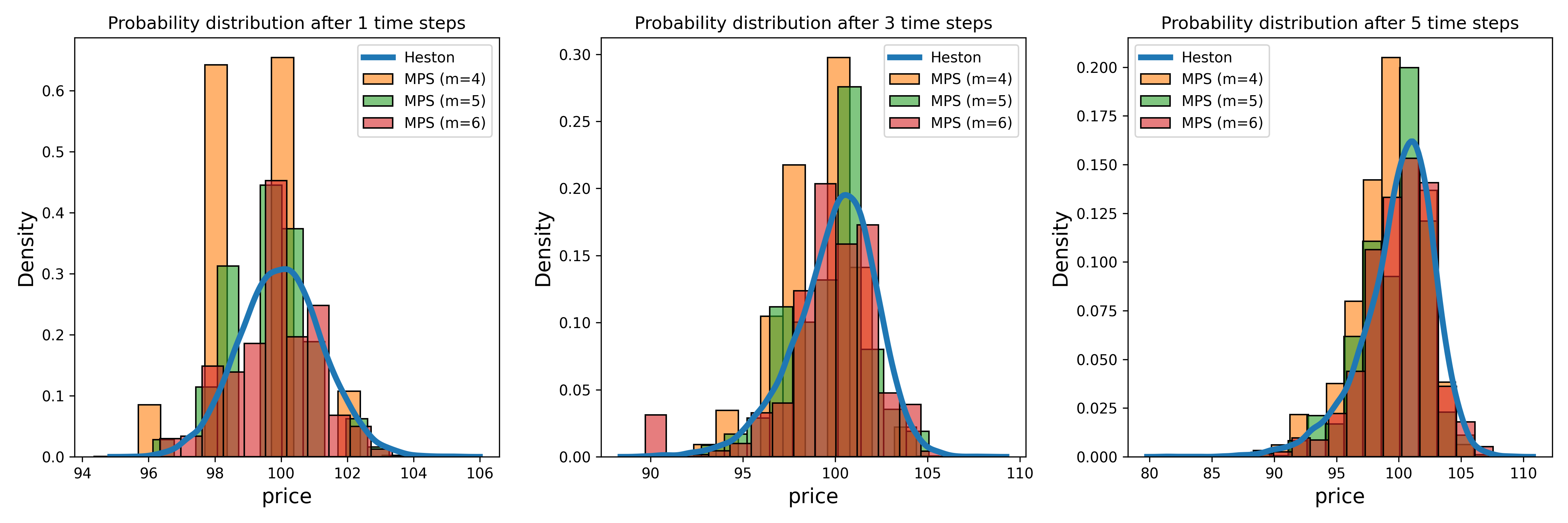
We first consider the effect of physical dimensions in MPS models. For that purpose, we fix and vary the physical dimensions with . Figure 1 shows the resulted probability distributions of , , and for each physical dimension. There, we plot empirical distributions of for samples generated by the Heston and MPS models. These figures indicate that the higher becomes the closer the distribution is to the Heston model. Note that, for , which means prices are discretized into only grid points, the resulting distribution is localized around several values, as in the left graph in Figure 1, but such a phenomenon is mitigated for larger .
| European | Asian | Lookback | Barrier | ||
|---|---|---|---|---|---|
| Price | IV | Price | Price | Price | |
| Heston | 1.1098 (0.0052) | 0.1967 (0.0009) | 0.6195 (0.0035) | 1.4778 (0.0056) | 0.9894 (0.0049) |
| MPS () | 0.6277 (0.0031) | 0.1113 (0.0005) | 0.2771 (0.0020) | 0.8216 (0.0030) | 0.5769 (0.0028) |
| MPS () | 0.8626 (0.0034) | 0.1529 (0.0009) | 0.4351 (0.0021) | 1.1625 (0.0039) | 0.8304 (0.0029) |
| MPS () | 1.0805 (0.0041) | 0.1915 (0.0007) | 0.6107 (0.0026) | 1.4612 (0.0049) | 0.9160 (0.0030) |
We then evaluate the price of options, and the IV calculated from the value of the European call option, showing the result in Table 1. Similarly to the probability distributions at each time step, with higher physical dimensions, option prices as well as the IV calculated by the MPS model get closer to those by the Heston model. On the European option, the IV by the MPS model with has a difference of several tenths of a percent from that by the Heston model, which we can say is practically a good fit for a pricing model of path-dependent options. Also for the Asian and lookback options, the prices by the MPS model are close to those by the Heston model with differences similar to that of the European option. Thus, we can conclude that the MPS model with sufficiently large physical dimension successfully learns the Heston model, at least for the purpose of pricing these options. On the other hand, for the barrier option, the difference between the prices of the two models is still larger even at . We may improve the MPS model by, e.g., taking larger or using tensor network architectures other than MPS, which can be considered in future works.
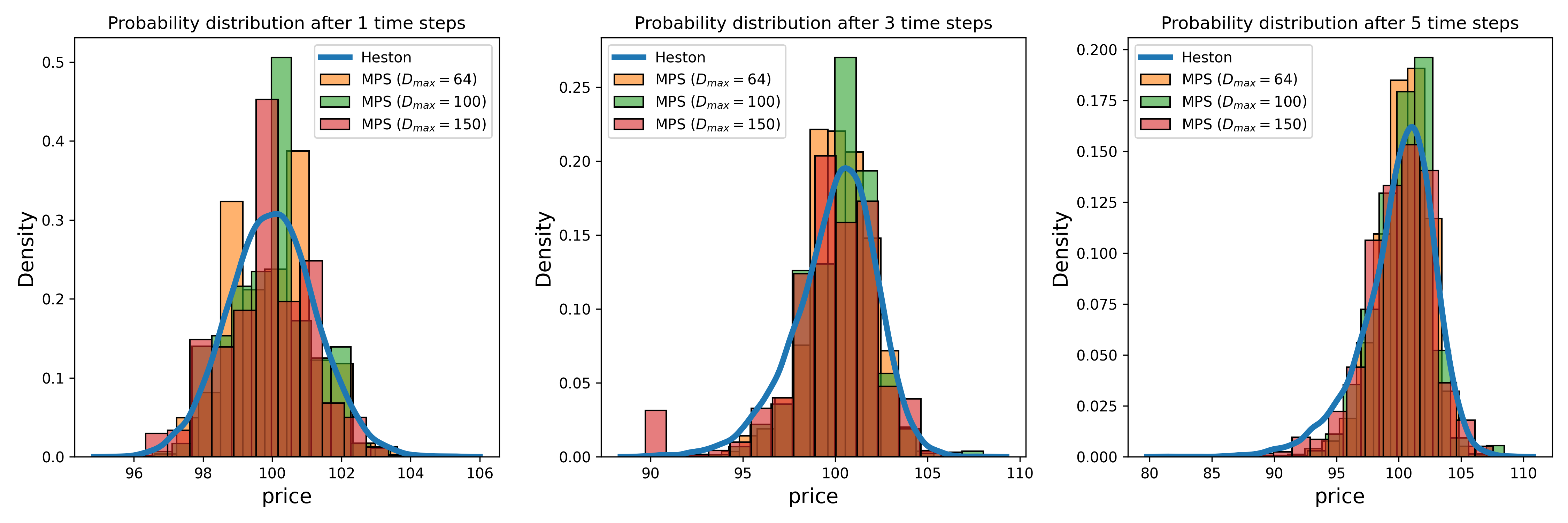
The MPS model has the other hyperparameter, which would be another factor for the model’s capability, that is, the maximal value of the bond dimension . In order to evaluate the effect of , we thus consider the different with fixed . In the below, we set . Figure 2 shows the probability distributions of for various . It is observed that with higher the distributions are closer to those of the Heston model. We also investigate the effect of in terms of option prices and the IV as shown in Table 2, where the results of the Heston and MPS models with are same as in Table 1. We find that, basically, the prices by the MPS model get closer to those by the Heston model as we increase . Only for the barrier option, the price difference becomes larger as increases, which implies that the MPS model underestimates its value possibly because the MPS model generates more paths that excess the barrier level, which largely affects the conditional expectation value for the barrier option, than the Heston model. The outliers in generated price paths can cause the discrepancy as well. These problems may be resolved by adopting some regularization technique to the model during training and generation, or by using tensor network structures other than MPS, which should be addressed in the future work.
| European | Asian | Lookback | Barrier | ||
|---|---|---|---|---|---|
| Price | IV | Price | Price | Price | |
| Heston | 1.1098 (0.0052) | 0.1967 (0.0009) | 0.6195 (0.0035) | 1.4778 (0.0056) | 0.9894 (0.0049) |
| MPS() | 0.9767 (0.0036) | 0.1731 (0.0006) | 0.5547 (0.0020) | 1.3270 (0.0036) | 0.9605 (0.0031) |
| MPS() | 1.0321 (0.0045) | 0.1829 (0.0008) | 0.5733 (0.0027) | 1.3701 (0.0047) | 0.9468 (0.0026) |
| MPS() | 1.0805 (0.0041) | 0.1915 (0.0007) | 0.6107 (0.0026) | 1.4612 (0.0049) | 0.9160 (0.0030) |
5 Conclusion
In this paper, we propose to utilize MPS for generating time series. Our primary concern is option pricing in quantitative finance where it is expected that quantum computing can accelerate the speed. To this end, we train the MPS model for the Heston model, which is common in the financial industry, and evaluate path-dependent options, using time series samples generated by the trained model. Our finding is that the proposed MPS model not only successfully generates price paths and probability distributions of the learned Heston model, but also calculate several path-dependent options using these samples with the Monte Carlo method.
We believe that our result sheds light on future implementation of quantum computing in finance, as MPS is naturally embedded into quantum circuits and can prepare quantum states for probability distributions of price paths for option pricing, as we show in this paper. We emphasize that our result differs from existing works in the sense that they focus on generating a probability distribution at some fixed time slice. Our work enables more flexible generation of time series samples, which gives us many potential applications and research directions. As a concluding remark, we comment some of them in the following.
While in this study we only consider the Heston model as a model of asset dynamics, there are other stochastic models used in the field of finance, such as the CEV model [45], SABR model [46], and so on. It would be interesting whether the MPS model can also reproduce these models’ dynamics. Another important issue is to implement our model in the quantum circuits, which might be difficult to do in the current environments, but should hopefully be possible in the future and reproduce our result. Additionally, it would be meaningful to conduct end-to-end implementation of option pricing in quantum computers with the combination of our MPS model and the Monte Carlo integration in quantum computing.
Acknowledgement
KM is supported by MEXT Quantum Leap Flagship Program (MEXT Q-LEAP) Grant no. JPMXS0120319794, JSPS KAKENHI Grant no. JP22K11924, and JST COI-NEXT Program Grant No. JPMJPF2014. The authors are grateful to Kosuke Mitarai for helpful discussions.
References
- [1] R. Orús, S. Mugel, and E. Lizaso, “Quantum computing for finance: Overview and prospects,” Reviews in Physics, vol. 4, p. 100028, 2019.
- [2] A. Bouland, W. van Dam, H. Joorati, I. Kerenidis, and A. Prakash, “Prospects and challenges of quantum finance,” arXiv preprint arXiv:2011.06492, 2020.
- [3] D. J. Egger, C. Gambella, J. Marecek, S. McFaddin, M. Mevissen, R. Raymond, A. Simonetto, S. Woerner, and E. Yndurain, “Quantum computing for finance: State-of-the-art and future prospects,” IEEE Transactions on Quantum Engineering, vol. 1, pp. 1–24, 2020.
- [4] D. Herman, C. Googin, X. Liu, A. Galda, I. Safro, Y. Sun, M. Pistoia, and Y. Alexeev, “A survey of quantum computing for finance,” arXiv preprint arXiv:2201.02773, 2022.
- [5] D. Herman, C. Googin, X. Liu, Y. Sun, A. Galda, I. Safro, M. Pistoia, and Y. Alexeev, “Quantum computing for finance,” Nature Reviews Physics, vol. 5, no. 8, pp. 450–465, 2023.
- [6] A. Montanaro, “Quantum speedup of monte carlo methods,” Proceedings of the Royal Society A: Mathematical, Physical and Engineering Sciences, vol. 471, no. 2181, p. 20150301, 2015.
- [7] G. Brassard, P. Hoyer, M. Mosca, and A. Tapp, “Quantum amplitude amplification and estimation,” Contemporary Mathematics, vol. 305, pp. 53–74, 2002.
- [8] P. Rebentrost, B. Gupt, and T. R. Bromley, “Quantum computational finance: Monte carlo pricing of financial derivatives,” Physical Review A, vol. 98, no. 2, p. 022321, 2018.
- [9] N. Stamatopoulos, D. J. Egger, Y. Sun, C. Zoufal, R. Iten, N. Shen, and S. Woerner, “Option pricing using quantum computers,” Quantum, vol. 4, p. 291, 2020.
- [10] K. Kaneko, K. Miyamoto, N. Takeda, and K. Yoshino, “Quantum pricing with a smile: implementation of local volatility model on quantum computer,” EPJ Quantum Technology, vol. 9, pp. 1–32, 2022.
- [11] L. Grover and T. Rudolph, “Creating superpositions that correspond to efficiently integrable probability distributions,” arXiv preprint quant-ph/0208112, 2002.
- [12] E. Muñoz Coreas and H. Thapliyal, “Everything you always wanted to know about quantum circuits,” Wiley Encyclopedia of Electrical and Electronics Engineering, pp. 1–17, 2022.
- [13] Y. R. Sanders, G. H. Low, A. Scherer, and D. W. Berry, “Black-box quantum state preparation without arithmetic,” Phys. Rev. Lett., vol. 122, p. 020502, Jan 2019.
- [14] S. Wang, Z. Wang, G. Cui, S. Shi, R. Shang, L. Fan, W. Li, Z. Wei, and Y. Gu, “Fast black-box quantum state preparation based on linear combination of unitaries,” Quantum Information Processing, vol. 20, no. 8, p. 270, 2021.
- [15] J. Bausch, “Fast Black-Box Quantum State Preparation,” Quantum, vol. 6, p. 773, Aug. 2022.
- [16] S. Wang, Z. Wang, R. He, S. Shi, G. Cui, R. Shang, J. Li, Y. Li, W. Li, Z. Wei, and Y. Gu, “Inverse-coefficient black-box quantum state preparation,” New Journal of Physics, vol. 24, p. 103004, oct 2022.
- [17] S. McArdle, A. Gilyén, and M. Berta, “Quantum state preparation without coherent arithmetic,” arXiv preprint arXiv:2210.14892, 2022.
- [18] A. G. Rattew and B. Koczor, “Preparing arbitrary continuous functions in quantum registers with logarithmic complexity,” arXiv preprint arXiv:2205.00519, 2022.
- [19] G. Marin-Sanchez, J. Gonzalez-Conde, and M. Sanz, “Quantum algorithms for approximate function loading,” Phys. Rev. Res., vol. 5, p. 033114, Aug 2023.
- [20] M. Moosa, T. W. Watts, Y. Chen, A. Sarma, and P. L. McMahon, “Linear-depth quantum circuits for loading fourier approximations of arbitrary functions,” Quantum Science and Technology, vol. 9, p. 015002, oct 2023.
- [21] C. Zoufal, A. Lucchi, and S. Woerner, “Quantum generative adversarial networks for learning and loading random distributions,” npj Quantum Information, vol. 5, no. 1, p. 103, 2019.
- [22] J. J. García-Ripoll, “Quantum-inspired algorithms for multivariate analysis: from interpolation to partial differential equations,” Quantum, vol. 5, p. 431, Apr. 2021.
- [23] K. Endo, T. Nakamura, K. Fujii, and N. Yamamoto, “Quantum self-learning monte carlo and quantum-inspired fourier transform sampler,” Phys. Rev. Res., vol. 2, p. 043442, Dec 2020.
- [24] A. Holmes and A. Y. Matsuura, “Efficient quantum circuits for accurate state preparation of smooth, differentiable functions,” in 2020 IEEE International Conference on Quantum Computing and Engineering (QCE), pp. 169–179, 2020.
- [25] F. Fuchs and B. Horvath, “A hybrid quantum wasserstein gan with applications to option pricing,” Available at SSRN 4514510, 2023.
- [26] A. Novikov, M. Trofimov, and I. Oseledets, “Exponential machines,” arXiv preprint arXiv:1605.03795, 2016.
- [27] E. Stoudenmire and D. J. Schwab, “Supervised learning with tensor networks,” Advances in neural information processing systems, vol. 29, 2016.
- [28] W. Huggins, P. Patil, B. Mitchell, K. B. Whaley, and E. M. Stoudenmire, “Towards quantum machine learning with tensor networks,” Quantum Science and technology, vol. 4, no. 2, p. 024001, 2019.
- [29] Z.-Y. Han, J. Wang, H. Fan, L. Wang, and P. Zhang, “Unsupervised generative modeling using matrix product states,” Physical Review X, vol. 8, no. 3, p. 031012, 2018.
- [30] S. Cheng, L. Wang, T. Xiang, and P. Zhang, “Tree tensor networks for generative modeling,” Physical Review B, vol. 99, no. 15, p. 155131, 2019.
- [31] J. Liu, S. Li, J. Zhang, and P. Zhang, “Tensor networks for unsupervised machine learning,” Physical Review E, vol. 107, no. 1, p. L012103, 2023.
- [32] S.-J. Ran, “Encoding of matrix product states into quantum circuits of one-and two-qubit gates,” Physical Review A, vol. 101, no. 3, p. 032310, 2020.
- [33] M. S. Rudolph, J. Miller, D. Motlagh, J. Chen, A. Acharya, and A. Perdomo-Ortiz, “Synergy between quantum circuits and tensor networks: Short-cutting the race to practical quantum advantage,” arXiv preprint arXiv:2208.13673, 2022.
- [34] M. S. Rudolph, J. Chen, J. Miller, A. Acharya, and A. Perdomo-Ortiz, “Decomposition of matrix product states into shallow quantum circuits,” Quantum Science and Technology, vol. 9, no. 1, p. 015012, 2023.
- [35] S. L. Heston, “A closed-form solution for options with stochastic volatility with applications to bond and currency options,” The review of financial studies, vol. 6, no. 2, pp. 327–343, 1993.
- [36] J. Hull, Options, futures, and other derivative securities, vol. 7. Prentice Hall Englewood Cliffs, NJ, 1993.
- [37] S. Shreve, Stochastic calculus for finance I: the binomial asset pricing model. Springer Science & Business Media, 2005.
- [38] S. E. Shreve et al., Stochastic calculus for finance II: Continuous-time models, vol. 11. Springer, 2004.
- [39] F. Black and M. Scholes, “The pricing of options and corporate liabilities,” Journal of political economy, vol. 81, no. 3, pp. 637–654, 1973.
- [40] R. C. Merton, “Theory of rational option pricing,” The Bell Journal of Economics and Management Science, vol. 4, no. 1, pp. 141–183, 1973.
- [41] B. Dupire et al., “Pricing with a smile,” Risk, vol. 7, no. 1, pp. 18–20, 1994.
- [42] J. C. Cox, J. E. Ingersoll Jr, and S. A. Ross, “A theory of the term structure of interest rates,” in Theory of valuation, pp. 129–164, World Scientific, 2005.
- [43] G. Maruyama, “Continuous markov processes and stochastic equations,” Rend. Circ. Mat. Palermo, vol. 4, pp. 48–90, 1955.
- [44] B. W. Silverman, Density estimation for statistics and data analysis. Routledge, 2018.
- [45] J. C. Cox, “The constant elasticity of variance option pricing model,” Journal of Portfolio Management, p. 15, 1996.
- [46] P. S. Hagan, D. Kumar, A. S. Lesniewski, and D. E. Woodward, “Managing smile risk,” Wilmott, vol. 1, pp. 84––108, 2002.