Direct Detection of Dark Photon Dark Matter with the James Webb Space Telescope

Abstract

In this study, we propose an investigation into dark photon dark matter (DPDM) within the infrared frequency band, utilizing highly sensitive infrared light detectors commonly integrated into space telescopes, such as the James Webb Space Telescope (JWST). The presence of DPDM induces electron oscillations in the reflector of these detectors. Consequently, these oscillating electrons can emit monochromatic electromagnetic waves with a frequency almost equivalent to the mass of DPDM. By employing the stationary phase approximation, we can demonstrate that when the size of the reflector significantly exceeds the wavelength of the electromagnetic wave, the contribution to the electromagnetic wave field at a given position primarily stems from the surface unit perpendicular to the relative position vector. This simplification results in the reduction of electromagnetic wave calculations to ray optics. By applying this concept to JWST, our analysis of observational data demonstrates the potential to establish constraints on the kinetic mixing between the photon and dark photon within the range [10, 500] THz. Despite JWST not being optimized for DPDM searches, our findings reveal constraints comparable to those obtained from the XENON1T experiment in the laboratory, as well as astrophysical constraints from solar emission. Additionally, we explore strategies to optimize future experiments specifically designed for DPDM searches.

I Introduction

The elusive nature of dark matter has thus far eluded detection through various non-gravitational search efforts. The scope of potential candidates has expanded beyond traditional weakly interacting massive particles (WIMPs) to encompass a broad range of mass scales. One intriguing category comprises ultralight bosonic dark matter, which has garnered significant attention as the lightest dark matter candidate. Among these, the dark photon is a notable ultralight vector dark matter candidate due to its kinetic mixing marginal operator coupling with the photon field, serving as one of the simplest extensions of the Standard Model Holdom (1986); Dienes et al. (1997); Abel and Schofield (2004); Abel et al. (2008a, b); Goodsell et al. (2009). The kinetic mixing dark photon could have been generated in the early universe and holds promise as a viable dark matter candidate Redondo and Postma (2009); Nelson and Scholtz (2011); Arias et al. (2012); Graham et al. (2016). Various mechanisms facilitate its plausibility, including the misalignment mechanism coupled with a non-minimal Ricci scalar coupling Nelson and Scholtz (2011); Arias et al. (2012); Alonso-Álvarez et al. (2019); Nakayama (2019, 2020), inflationary fluctuations Graham et al. (2016); Ema et al. (2019); Kolb and Long (2021); Salehian et al. (2021); Ahmed et al. (2020); Nakai et al. (2020); Nakayama and Tang (2020); Kolb and Long (2021); Salehian et al. (2021); Firouzjahi et al. (2021); Bastero-Gil et al. (2022); Firouzjahi et al. (2022); Sato et al. (2022), parametric resonances Co et al. (2018); Dror et al. (2018); Bastero-Gil et al. (2018); Agrawal et al. (2018); Co et al. (2021); Nakayama and Yin (2021), or the decay of cosmic strings Long and Wang (2019).

Due to the vast range of unknown mass of the dark photon dark matter (DPDM), there are various detecting methods accordingly Fabbrichesi et al. (2020); Caputo et al. (2021). The relevant searches for dark photon DM are haloscope experiments De Panfilis et al. (1987); Wuensch et al. (1989); Hagmann et al. (1990); Asztalos et al. (2001, 2010); Hoang Nguyen et al. (2019), dish antenna experiments Horns et al. (2013); Jaeckel and Redondo (2013a); Jaeckel and Knirck (2016); Knirck et al. (2018), plasma telescopes Gelmini et al. (2020), CMB spectrum distortion Arias et al. (2012); McDermott and Witte (2020) and radio telescopes An et al. (2021, 2023a, 2023b). The searches include direct detection of local DPDM in laboratories and observation on its impact in the early universe.

Recently, we proposed to search for Dark Photon Dark Matter (DPDM) conversion, specifically $A^{\prime}\to\gamma$, locally using radio telescopes such as FAST and LOFAR An et al. (2023a). For instance, the FAST radio telescope, equipped with a large dish antenna, converts DPDM into a regular photon field. In each small surface area of FAST, an oscillating electric dipole is generated by the DPDM field, with a frequency matching the DPDM mass. Summing up the contributions from each surface area yields the total converted electromagnetic field. The original proposal utilized a spherical reflector, causing the electromagnetic field to constructively focus on the spherical center Horns et al. (2013); Jaeckel and Redondo (2013b); Jaeckel and Knirck (2016). This concept has been previously employed in shielded room-sized experiments by various works, utilizing variations such as plane/parabolic reflectors or dipole antennas Suzuki et al. (2015a, b); Knirck et al. (2018); Tomita et al. (2020); Godfrey et al. (2021); Brun et al. (2019); Andrianavalomahefa et al. (2020); Bajjali et al. (2023).

In this article, we would like to explore this idea with the recent new telescope, the James Webber Science Telescope (JWST), which is running in space. JWST covers the frequency range of 10–500 THz for infrared astronomy. Our searches for DPDM benefit from JWST’s high frequency resolution $R=f/\Delta f$, which ranges from 4 to 3000, depending on different obervation modes Gardner et al. (2006). Also, since it works in space, we expect it to have a much lower noise background than terrestrial facilities. The Near Infrared Spectrograph (NISpec) and the Mid-Infrared Instrument (MIRI), two instruments carried by JWST, are especially useful for searching for DPDM. By analyzing data collected by the two instruments, we get the upper limits for the DPDM-photon coupling constant, $\epsilon\sim 10^{-10}-10^{-12}$ in the frequency range $10-500$ THz at $95\%$ confidence level (C.L.).

The Lagrangian of the dark photon model in this work is a vector boson that couples to the SM particles through its kinetic mixing with photon, and the Lagrangian is described by the equation

$$\mathcal{L}=-\frac{1}{4}F^{\prime}_{\mu\nu}F^{\prime\mu\nu}+\frac{1}{2}m_{A^{\prime}}^{2}A^{\prime}_{\mu}A^{\prime\mu}-\frac{1}{2}\epsilon F_{\mu\nu}F^{\prime\mu\nu}\ ,$$ (1)

where $F$ and $F^{\prime}$ are the dark photon and photon field strength, $\epsilon$ is the kinematic mixing. After proper rotation and redefinition, one can eliminate the kinematic mixing term and arrive at the interaction Lagrangian for $A^{\prime}$, the SM photon $A$, and the electromagnetic current $j_{\rm em}^{\mu}$,

$$\mathcal{L}_{\rm int}=ej_{\rm em}^{\mu}(A_{\mu}-\epsilon A^{\prime}_{\mu})\ ,$$ (2)

where $e$ is the electromagnetic coupling. Therefore, the DPDM electric field, $\bm{E}^{\prime}=-\dot{\bm{A}}^{\prime}-\nabla A^{\prime 0}$, can accelerate the charge carriers in a reflector and thus be converted to SM electromagnetic waves.

This work is structured as follows: In Section I, we present the background of DPDM conversion. In Section II, we offer a mathematical proof of the reduction from complex electroweak wave calculation to ray optics using the stationary phase approximation. Section III applies the simplified calculation to JWST, obtaining the equivalent flux density of the electromagnetic field in Section IV. Section V establishes limits on the kinetic mixing parameter of the dark photon using JWST observational data. Finally, in Section VI, we draw our conclusions.

II High Frequency Approximation

In order to calculate the EM signals induced by DPDM on a metal reflector plate, the most direct way is to divide the reflector into many small patches and sum up the induced EM signals over all of them. The length of each small patch is required to be much smaller than the wavelength $\lambda$ of the induced EW signal while at the same time much larger than the reflector thickness. Consequently, to ensure enough accuracy, the simulation mesh must be fine enough for the distance between mesh points to be smaller than the wavelength. This method works well in the case of FAST telescope An et al. (2023c). The FAST detects radio photons around $1$ GHz and has a reflector roughly $500$ m in diameter. Therefore, we only need to divide the FAST reflector into $\sim 10^{6}$ patches for an accurate simulation. On the other hand, JWST works at a much higher frequency range, $10-500$ THz (i.e., the photon wavelength $\lambda\sim 0.6-30\leavevmode\nobreak\ \mathrm{\mu m}$), and the diameter of the JWST’s primary mirror is $D=6.6$ meter. To achieve an acceptable level of accuracy in simulating the JWST case, we require over $10^{15}$ patches, which is finer than the FAST case by orders of magnitude. However, such a fine mesh imposes an immense computational burden, rendering it unfeasible to simulate signal strength using available computer resources.

Fortunately, as we will see, we can theoretically demonstrate that calculating the induced EM signals becomes considerably more straightforward in the high-frequency regime, $D\gg\lambda$. Similar to the case of reaching the ray optics at the high-frequency limit of the wave optics, we can establish that the strength of the DPDM-induced signal can be obtained using a ray-optical method. This simplification ultimately leads to a set of algebraic equations that can be easily calculated, even manually without the need of a fine-mesh simulation. The physical interpretation of such a simplification is that, in the high-frequency regime, interferences between different patches on the reflector have a negligible impact on the final result.

To be more specific, this simplification works primarily due to two key factors. Firstly, the phases of the electric fields contributed by different patches on a plate vary significantly, while their strengths remain relatively the same. This results in significant cancellations between the electric fields generated by different patches. Secondly, one significant parameter is the coherence length of DPDM. The DPDM and the induced photon have the same energy, but the coherent length of DPDM, $\lambda^{\prime}$, is much larger than the wavelengh of the induced photons, $\lambda$. This is due to the non-relativistic nature of dark matter with a low speed $v_{\rm DM}\sim 10^{-3}$, which gives $\lambda^{\prime}\sim\lambda/v_{\rm DM}$. Importantly, $\lambda^{\prime}$ is still significantly smaller than the diameter of the JWST’s mirrors. As a result, the interferences between different patches are dampened by incoherence.

In the following, we are going to prove that the ray optics is indeed applicable here in calculating the EM signals induced by DPDM for the JWST case which locates in the high-frequency regime, $D/\lambda\sim 10^{6}$ and $D/\lambda^{\prime}\sim 10^{3}$. Finally, a formula for computing the strength of the induced signal will be introduced.

II.1 Monochromatic DPDM

Firstly, we consider a simplified case that DPDM is monochromatic in frequency. Then, in the next subsection, we discuss the more realistic case where the velocity distribution of dark matter is included. Under the effect of the DPDM’s dark electric field, each small patch on a reflector plate can be treated as an electric dipole,

$$\bm{p}=2\epsilon\bm{A^{\prime}}_{\bm{\tau}}\Delta S,$$ (3)

where $\bm{A^{\prime}}_{\bm{\tau}}$ is the component of $\bm{A^{\prime}}$ parallel with the patch and $\Delta S$ is the area of the patch An et al. (2023c). The dipole is oscillating as a result of the oscillation of the DPDM field. Then, summing up the EM radiations from all the dipoles, we arrive at the expressions of the induced EM fields at position $\bm{r}$ An et al. (2023c),

$$\bm{E}(\bm{r}) =-\frac{\epsilon m_{A^{\prime}}^{2}|\bm{A}^{\prime}|}{2\pi}\int[\bm{\tau}\times(\bm{r}-\bm{r}^{\prime})]\times(\bm{r}-\bm{r}^{\prime})\frac{e^{im_{A^{\prime}}|\bm{r}-\bm{r}^{\prime}|+i\bm{k}^{\prime}\cdot(\bm{r}^{\prime}-\bm{r})}}{|\bm{r}-\bm{r}^{\prime}|^{3}}\mathrm{d}S^{\prime},$$ (4)

$$\bm{B}(\bm{r}) =-\frac{\epsilon m_{A^{\prime}}^{2}|\bm{A}^{\prime}|}{2\pi}\int\bm{\tau}\times(\bm{r}-\bm{r}^{\prime})\frac{e^{im_{A^{\prime}}|\bm{r}-\bm{r}^{\prime}|+i\bm{k}^{\prime}\cdot(\bm{r}^{\prime}-\bm{r})}}{|\bm{r}-\bm{r}^{\prime}|^{2}}\mathrm{d}S^{\prime}.$$ (5)

$\bm{k}^{\prime}$ is the wave vector of DPDM. $\bm{A^{\prime}}_{\bm{\tau}}=\bm{\tau}|\bm{A^{\prime}}|$ where the tangent vector $\bm{\tau}$ can be calculated as $\bm{\tau}\equiv\bm{n}_{0}-(\bm{n}_{0}\cdot\bm{n})\bm{n}$. The two unit vectors, $\bm{n}_{0}$ and $\bm{n}$, represent the direction of $\bm{A}^{\prime}$ and the normal direction of ${\rm d}S$, respectively. The magnitude of oscillations, $|\bm{A}^{\prime}|$, is determined by the dark matter energy density $\rho_{\rm DM}$, that is,

$$\rho_{\rm DM}=\frac{1}{2}m_{A^{\prime}}^{2}|\bm{A^{\prime}}|^{2}=\frac{1}{2}|\bm{E^{\prime}}|^{2}.$$ (6)

Then, we can calculate the energy flux density,

$$\langle\bm{S^{\prime}}\rangle_{t}=\frac{1}{2}\mathrm{Re}(\bm{E}\times\bm{B^{*}}).$$ (7)

$\left<...\right>_{t}$ here means the average over time. In principle, for any reflectors, we can numerically simulate the DPDM-induced EM waves using these formulas. However, as we discussed above, such a simulation requires a very fine mesh that is hard to realize in computers for the JWST case. As we are going to see below, we figure out a more analytical method applicable in the high-frequency regime.

The key to simplifying our formulas in the high-frequency regime is to use the stationary phase approximation. In general, the stationary phase approximation works in solving the following integral as $\alpha$ tends to infinity Bleistein and Handelsman (1986),

$$\int_{\mathbb{R}^{n}}g(\bm{x})e^{i\alpha f(\bm{x})}\mathrm{d}^{n}\bm{x}$$

$$=\sum_{\bm{x}_{0}\in\Sigma}e^{i\alpha f(\bm{x}_{0})}|\det(\mathrm{Hess}(f(\bm{x}_{0})))|^{-1/2}e^{\frac{i\pi}{4}\mathrm{sgn}(\mathrm{Hess}(f(\bm{x}_{0})))}\left(\frac{2\pi}{\alpha}\right)^{\frac{n}{2}}g(\bm{x}_{0})+o(\alpha^{-\frac{n}{2}}),\ \alpha\rightarrow\infty.$$ (8)

where the function $g(\bm{x})$ is either zero or exponentially suppressed when $\bm{x}$ is large, (the condition where $g(\bm{x})$ is zero when $\bm{x}$ is large, can be more accurately described by the mathematical terminology of “compactly supported”). $\Sigma$ is the set of points where $\nabla f=0$. $\mathrm{Hess}(f(x_{0}))$ is the Hessian of $f$, and $\mathrm{sgn}(\mathrm{Hess}(f(\bm{x}_{0})))$ is the signature of the Hessian,

$${\rm Hess}(f(\bm{x}_{0}))_{ij}=\left.\frac{\partial^{2}f}{\partial x_{i}\partial x_{j}}\right|_{\bm{x}=\bm{x}_{0}},$$ (9)

$${\rm sgn}({\rm Hess}(f(\bm{x}_{0})))=\sharp({\rm positive\ eigenvalues})-\sharp({\rm negative\ eigenvalues}).$$ (10)

Note that Eq. (8) is only valid when we assume $\nabla f=0$ has only discrete solutions, otherwise $\mathrm{Hess}(f(x_{0}))$ is non-degenerate at $x_{0}\in\Sigma$.

This stationary-phase approximation (8) can be intuitively understood in the following way: when $k$ is large, the exponential oscillates rapidly with a small change of $\bm{x}$, while $g(\bm{x})$ changes very little. Therefore, the integral vanishes unless we are considering a small patch in $\mathbb{R}^{n}$ around $\nabla f=0$, which is the stationary point of the phase factor. A rigorous proof of Eq. (8) is provided in Appendix B.

In the JWST case, the phase factor is $m_{A^{\prime}}|\bm{r}-\bm{r}^{\prime}|+\bm{k}^{\prime}\cdot(\bm{r}^{\prime}-\bm{r})$. Given that the dark photon’s wave vector is approximately $10^{-3}$ times its frequency, the phase factor is dominated by the first term. By rewriting the first term as $m_{A^{\prime}}D\times(|\bm{r}-\bm{r}^{\prime}|/D)$, with $D$ being the characteristic length of JWST optical elements, the second factor becomes an $\mathcal{O}(1)$ function of spacial coordinates, and $m_{A^{\prime}}D\gg 1$ by assumption. This is equivalent to the case $\alpha\gg 1$ in Eq. (8). Consequently, we can apply the stationary-phase approximation (8) to calculate Eq. (4). The process of calculating Eq. (5) is the same, so it will not be shown here for the sake of conciseness. In the most general setup, a conductor is a closed surface. In Eq. (4), the domain of integration is the whole conductor surface. By assumption, this integral can be split into several integrals in compact subsets of $\mathbb{R}^{2}$, with the surface element $\mathrm{d}S$ re-expressed in the form $J(\bm{r}^{\prime})\mathrm{d}u\mathrm{d}v$ where $J$ is the Jacobian determined by the equation of the surface. We study each of these integrals separately, and denote by $\Omega$ the domain of integration. Define

$$g(\bm{r^{\prime}})=\begin{cases}-\dfrac{\epsilon m_{A^{\prime}}^{2}|\bm{A^{\prime}}|}{2\pi}\dfrac{[\bm{\tau}(\bm{r^{\prime}})\times(\bm{r}-\bm{r^{\prime}})]\times(\bm{r}-\bm{r^{\prime}})}{|\bm{r}-\bm{r^{\prime}}|^{3}}J(\bm{r}^{\prime})&\bm{r^{\prime}}\in\Omega\\ 0&\bm{r^{\prime}}\notin\Omega\end{cases}.$$ (11)

Clearly, $g(\bm{r}^{\prime})$ is compactly supported. Applying the stationary phase approximation, the only contribution to the integral comes from points where

$$\frac{\partial}{\partial u}|\bm{r}-\bm{r^{\prime}}(u,v)|=0,\leavevmode\nobreak\ \leavevmode\nobreak\ \leavevmode\nobreak\ \frac{\partial}{\partial v}|\bm{r}-\bm{r^{\prime}}(u,v)|=0,$$ (12)

or equivalently,

$$(\bm{r}-\bm{r^{\prime}})\cdot\frac{\partial\bm{r}^{\prime}}{\partial u}=0,\leavevmode\nobreak\ \leavevmode\nobreak\ \leavevmode\nobreak\ (\bm{r}-\bm{r^{\prime}})\cdot\frac{\partial\bm{r}^{\prime}}{\partial v}=0.$$ (13)

$u$ and $v$ can be understood as two parameters describing a certain patch of the surface, so $\partial\bm{r}^{\prime}/\partial u$ and $\partial\bm{r}^{\prime}/\partial v$ are tangent vectors at $\bm{r}^{\prime}$. Therefore, Eq. (13) tells us that $\bm{r}-\bm{r}^{\prime}$ is perpendicular to the tangent plane at $\bm{r}^{\prime}$. This result can be interpreted in a more intuitive way. Considering a conductor surface, at each point $\bm{r}^{\prime}$ on the surface, a light ray is only emitted in the normal direction, then the signal received at the position $\bm{r}$ is the sum of the light rays passing through the position $\bm{r}$. Therefore, we see the calculations in the JWST case can be accomplished within the framework of ray optics. The key difference with conventional ray optics is that a light ray induced by DPDM is always perpendicular to the local surface from which it is emitted, regardless of the direction in which the DPDM is incident.

We denote by $\hat{\bm{r}}_{j}$ the $j$th point on the conductor surface such that $\bm{r}-\hat{\bm{r}}_{j}$ is perpendicular to the tangent plane at $\hat{\bm{r}}_{j}$. Using the stationary-phase method, Eq. (4) becomes

$$\bm{E}(\bm{r})=\sum_{j}ie^{im_{A^{\prime}}|\bm{r}-\hat{\bm{r}}_{j}|}\epsilon m_{A^{\prime}}\hat{\bm{A}}^{\prime}(\hat{\bm{r}}_{j})$$ (14)

where $\hat{\bm{A}}^{\prime}(\hat{\bm{r}}_{j})=|\bm{A}^{\prime}|\bm{\tau}(\hat{\bm{r}}_{j})$ is the projection of $\bm{A}^{\prime}$ onto the tangent plane at $\hat{\bm{r}}_{j}$. The expression for $\bm{B}$ is similar which is not present here for the purpose of conciseness. Putting everything together, we get

$$\langle\bm{S}(\bm{r})\rangle_{t}=\sum_{j}\frac{1}{2}\epsilon^{2}m_{A^{\prime}}^{2}\hat{\bm{A^{\prime}}}(\hat{\bm{r}}_{j})^{2}\hat{\bm{n}}(\hat{\bm{r}}_{j})+\mbox{interference terms}$$ (15)

where $\hat{\bm{n}}(\hat{\bm{r}}_{j})$ is the out-pointing normal direction of the conductor surface at $\hat{\bm{r}}_{j}$. The interference term comes from the cross products of contributions from $\hat{\bm{r}}_{j}$ and $\hat{\bm{r}}_{k}$, with $j\neq k$. If there is only one $\hat{\bm{r}}_{j}$, there is only one term in the summation and the interference term drops out. As a consistency check, one can compare (15) with the result of infinitely large metal plate given in appendix I-A of Ref. An et al. (2023c).

In the most extreme case, the conductor is a sphere and the detector is placed at the center of the sphere. Then, for the detector, the phase is stationary everywhere on the sphere and no simplification can be made to Eqs. (4) and (5). Note that this is not the case with JWST, because the reflectors in JWST are not spherical, and the points $\hat{\bm{r}}_{j}$ are indeed discrete. In addition, in the frequency range of JWST, the correlation length is much smaller than the characteristic length of the reflectors, and the interference between different patches is further suppressed. This will be discussed in more detail in the following section.

II.2 Non-monochromatic DPDM

According to the Standard Halo Model, dark matter has a truncated Maxwellian distribution in the momentum space. Consequently, we should take into consideration the effect of finite coherence length of DPDM. The dark photon field at a location $\bm{x}$ can be expressed as,

$$\bm{E^{\prime}}(\bm{x},t)=\int_{<k_{\mathrm{esc}}}\frac{\mathrm{d}^{3}\bm{k}^{\prime}}{(2\pi)^{3}}be^{-\frac{\bm{k}^{\prime 2}}{k_{0}^{2}}}\times\bm{E^{\prime}}_{0}e^{i(\bm{k}^{\prime}\cdot\bm{x}-\omega t+\theta(\bm{k}^{\prime}))}$$ (16)

where $\theta(\bm{k}^{\prime})$ is a random phase associated with the $\bm{k}^{\prime}$ mode and $\omega=\sqrt{\bm{k}^{\prime 2}+m_{A^{\prime}}^{2}}$ is the energy. $b$ is a normalization factor. We have $k_{0}=m_{A^{\prime}}v_{0}$ and $k_{\mathrm{esc}}=m_{A^{\prime}}v_{\mathrm{esc}}$, where $v_{0}\approx$235\text{\,}\mathrm{k}\mathrm{m}\mathrm{/}\mathrm{s}$$ is the most probable velocity and $v_{\mathrm{esc}}$ is the escape velocity of leaving the Galaxy at the position of the solar system which is about $500\leavevmode\nobreak\ {\rm km/s}$ Drukier et al. (1986); Evans et al. (2019). Due to randomness, we assume that there is no correlation between different momentum modes,

$$\langle e^{i(\theta(\bm{k}^{\prime}_{1})-\theta(\bm{k}^{\prime}_{2}))}\rangle_{t}=a(2\pi)^{3}\delta^{3}(\bm{k}^{\prime}_{1}-\bm{k}^{\prime}_{2})$$ (17)

where $a$ is a dimensionful constant. Then, analogous to Eqs. (4) and (5), the full expressions for the induced electric and magnetic fields read

$$\bm{E}=-\int_{<k_{\mathrm{esc}}}\frac{\mathrm{d}^{3}\bm{k}^{\prime}}{(2\pi)^{3}}\frac{\epsilon m_{A^{\prime}}|\bm{E}^{\prime}_{0}|}{2\pi}be^{-\frac{\bm{k}^{\prime 2}}{k_{0}^{2}}}\int\mathrm{d}S^{\prime}[\bm{\tau}(\bm{r^{\prime}})\times(\bm{r}-\bm{r^{\prime}})]\times(\bm{r}-\bm{r^{\prime}})\frac{e^{i(\omega|\bm{r}-\bm{r^{\prime}}|+\bm{k}^{\prime}\cdot\bm{r^{\prime}}+\theta(\bm{k}^{\prime}))}}{|\bm{r}-\bm{r^{\prime}}|^{3}},$$ (18)

$$\bm{B}=-\int_{<k_{\mathrm{esc}}}\frac{\mathrm{d}^{3}\bm{k}^{\prime}}{(2\pi)^{3}}\frac{\epsilon m_{A^{\prime}}|\bm{E}^{\prime}_{0}|}{2\pi}be^{-\frac{\bm{k}^{\prime 2}}{k_{0}^{2}}}\int\mathrm{d}S^{\prime}\bm{\tau}(\bm{r^{\prime}})\times(\bm{r}-\bm{r^{\prime}})\frac{e^{i(\omega|\bm{r}-\bm{r^{\prime}}|+\bm{k}^{\prime}\cdot\bm{r^{\prime}}+\theta(\bm{k}^{\prime}))}}{|\bm{r}-\bm{r^{\prime}}|^{2}}.$$ (19)

One can further obtain the full expression for the energy flux density,

$$\langle\bm{S}\rangle_{t}=\frac{1}{2}\int_{<k_{\mathrm{esc}}}\frac{\mathrm{d}^{3}\bm{k}^{\prime}}{(2\pi)^{3}}\left(\frac{\epsilon m_{A^{\prime}}|\bm{E}^{\prime}_{0}|}{2\pi}\right)^{2}ab^{2}e^{-\frac{2\bm{k}^{\prime 2}}{k_{0}^{2}}}\int\mathrm{d}S^{\prime}\mathrm{d}S^{\prime\prime}\left\{\left[\bm{\tau}(\bm{r^{\prime}})\times(\bm{r}-\bm{r^{\prime}})\right]\times(\bm{r}-\bm{r^{\prime}})\right\}$$

$$\times[\bm{\tau}(\bm{r^{\prime\prime}})\times(\bm{r}-\bm{r^{\prime\prime}})]\mathrm{Re}\left(\frac{e^{im_{A^{\prime}}(|\bm{r}-\bm{r^{\prime}}|-|\bm{r}-\bm{r^{\prime\prime}}|)+i\bm{k}^{\prime}\cdot(\bm{r^{\prime}}-\bm{r^{\prime\prime}})}}{|\bm{r}-\bm{r^{\prime}}|^{3}|\bm{r}-\bm{r^{\prime\prime}}|^{2}}\right).$$ (20)

This expression can be simplified after some computation, the detail is given in appendix A.

$$\langle\bm{S}\rangle_{t}=\rho_{\mathrm{DM}}\left(\frac{\epsilon}{\lambda}\right)^{2}\int\mathrm{d}S^{\prime}\mathrm{d}S^{\prime\prime}\left\{\left[\bm{\tau}(\bm{r^{\prime}})\times(\bm{r}-\bm{r^{\prime}})\right]\times(\bm{r}-\bm{r^{\prime}})\right\}\times[\bm{\tau}(\bm{r^{\prime\prime}})\times(\bm{r}-\bm{r^{\prime\prime}})]$$

$$\times e^{-\frac{1}{8}k_{0}^{2}|\bm{r^{\prime}}-\bm{r^{\prime\prime}}|^{2}}\mathrm{Re}\left(\frac{e^{im_{A^{\prime}}(|\bm{r}-\bm{r^{\prime}}|-|\bm{r}-\bm{r^{\prime\prime}}|)}}{|\bm{r}-\bm{r^{\prime}}|^{3}|\bm{r}-\bm{r^{\prime\prime}}|^{2}}\right)$$ (21)

If we choose the reflector to be spherical, some analytic results can be derived. In the $k_{0}\rightarrow 0$ limit, i.e. the infinite correlation length limit, the result is

$$\frac{\langle\bm{S}\rangle_{t}}{\rho_{\mathrm{DM}}}=\frac{1}{3}\pi^{2}\epsilon^{2}\frac{R^{2}}{\lambda^{2}}s_{\gamma}s_{\theta_{0}}^{2}\sqrt{c_{\gamma}^{2}(2-3c_{\theta_{0}}+c_{\theta_{0}}^{3})^{2}+4s_{\gamma}^{2}(c_{\theta_{0}}^{3}-1)^{2}}$$ (22)

where $\gamma$ is the angle between the polarization vector $\bm{n}_{0}$ and z-direction, $\theta_{0}$ describes how large the spherical surface is, with $\theta_{0}=0$ for the surface shrinking to a point and $\theta_{0}=\pi$ for the surface becoming a full sphere. This is the same as what we obtained in An et al. (2023c). We are also interested in the $k_{0}\rightarrow\infty$ limit, i.e. the zero correlation length limit, the result is

$$\frac{\langle\bm{S}\rangle_{t}}{\rho_{\mathrm{DM}}}=\frac{\epsilon^{2}}{2v_{0}^{2}}s_{\theta_{0}}^{2}\sqrt{4s_{\gamma}^{2}c_{\gamma}^{2}s_{\theta_{0}}^{4}+(2(1+c_{\theta_{0}}^{2})s_{\gamma}^{2}+(1+c_{\gamma}^{2})s_{\theta_{0}}^{2})^{2}}$$ (23)

Interestingly, the flux in the high frequency limit doesn’t depend on the radius of the sphere, but it does depend on $\theta_{0}$. Note that (23) only applies when the radius of the reflector is much larger than the dark photon wavelength, which is $10^{3}$ times the same-frequency EM wavelength. Naively, larger reflectors produce stronger signal, but (23) tells us that the signal saturates when the reflector is much larger than the dark photon wavelength.

Coming back to the JWST case, we apply again the stationary phase approximation. In order that the integration is not suppressed, $\bm{r}^{\prime}$ has to satisfy two conditions:

$$\bm{r}-\bm{r}^{\prime}\perp\mbox{tangent plane at }\bm{r}^{\prime},\quad\bm{r}^{\prime}=\bm{r}^{\prime\prime}$$ (24)

This means that due to finite correlation length, the contribution from interference terms completely vanishes. We denote by $\hat{\bm{r}}_{i}$ the $i$th solution to the perpendicular condition (24), and the total flux density is,

$$\langle\bm{S}(\bm{r})\rangle_{t}=\sum_{i}\frac{1}{2}\epsilon^{2}m_{A^{\prime}}^{2}\hat{\bm{A^{\prime}}}^{2}(\hat{\bm{r}}_{i})\hat{\bm{n}}(\hat{\bm{r}}_{i})$$ (25)

Again, $\hat{\bm{n}}(\hat{\bm{r}}_{i})$ is the out-directed normal vector at $\hat{\bm{r}}_{i}$, and $\hat{\bm{A^{\prime}}}(\hat{\bm{r}}_{i})=|\bm{A}^{\prime}|\bm{\tau}(\hat{\bm{r}}_{i})$. Note that if the set of solutions to (24) is not discrete, we should change the sum into an integration. If one wishes to average over all possible polarization, the result is

$$\langle\bm{S}(\bm{r})\rangle_{t}=\sum_{i}\frac{2}{3}\epsilon^{2}\rho_{\rm DM}(\hat{\bm{r}}_{i})\hat{\bm{n}}(\hat{\bm{r}}_{i})$$ (26)

In the JWST case, all approximation conditions applied in this section are satisfied, so one may directly use (26) to compute the dark photon flux density.

III The Optical Telescope Element (OTE) of JWST

The Optical Telescope Element (OTE) of the James Webb Space Telescope (JWST) comprises a primary mirror, a secondary mirror, a tertiary mirror, and a fine steering mirror. A sketch of the mirror system is shown in Figure 1. Detailed parameters for these optical components are available in JWST documentation Lightsey et al. (2012), and we have also summarized them in Table 1.

Component	RoC(mm)	Surface	Conic	$V_{1}$(mm)	$V_{2}$(mm)	$V_{3}$(mm)	Size(mm)
Primary	15879.7	concave	-0.9967	0	0	0	6605.2(diameter)
Secondary	1778.9	convex	-1.6598	7169.0	0	0	738(diameter)
Tertiary	3016.2	concave	-0.6595	-796.3	0	-0.19	728(length)$\times$517(width)
Fine Steering Mirror		flat		1047.8	0	-2.36	172.5(diameter)

Table 1: Parameters for the optical elements of JWST. The data can be found in JWST documentation Lightsey et al. (2012).

In the table, ‘RoC’ denotes the radius of curvature, and ‘conic’ denotes the conic constant $K$ which can be related to eccentricity $e_{\mathrm{cone}}$ as

$$K=-e_{\mathrm{cone}}^{2}.$$ (27)

Figure 1: The OTE of JWST. Everything is drawn to scale. Figure taken from Ref. Gardner et al. (2006).

Table 1 provides insights into the optical characteristics of the JWST’s optical elements. The primary and tertiary mirrors exhibit elliptical shapes, while the secondary mirror is hyperbolic and the fine steering mirror is flat. The primary, secondary and fine steering mirrors are rounded, while the tertiary mirror is rectangularLightsey et al. (2014). Their sizes are listed in Table 1. $V_{1}$, $V_{2}$ and $V_{3}$ are the spacial displacements of the mirrors, as shown in Fig. 1.

The EM energy flux density induced by DPDM originates from several sources within the optical system. DPDM can interact with different components of the optical train, including the primary mirror. The light emitted from the primary mirror is then sequentially reflected by the secondary mirror, the tertiary mirror, and the fine steering mirror before reaching the detector. Additionally, DPDM can also directly interact with the secondary mirror, leading to a ‘double’ reflection before being detected. The same principle applies to interactions with the tertiary and fine steering mirrors. However, it is important to note that not all the lights induced by DPDM on the mirrors will reach the detector. Some of them may stray and cannot be focused on the detector after multiple reflections between the mirrors. After all, the JWST mirror system is designed to focus parallel lights from distant sources, while our light rays are always perpendicular to the mirror surface at which they are induced. To quantify the amount of the induced flux that can reach the detector, a detailed analysis of light propagation within the mirror system is necessary.

In the following section, we are going to carry out such an analysis based on the ray-transfer-matrix method. This method is applicable when the paraxial condition is satisfied, which means that the rays should be within a small angle to the optical axis throughout the system. We will show that the paraxial condition is indeed met in our case. It’s important to note that while the mirrors’ absolute sizes may not be significantly smaller than their radii of curvature, their effective sizes are small so that can satisfy the paraxial condition. Here, ‘effective’ refers to the portion of the mirror surface that make contributions to the flux finally detected.

IV Calculating the Equivalent Flux Density

In this section, we are going to use the ray-transfer-matrix method to calculate the induced flux that can finally be detected by the JWST detector. A technical review of the ray-transfer-matrix method is shown in Appendix C. Firstly, we can alter the direction of light rays to make them move to the right for convenience, while at the same time we replace each reflector with a corresponding type of lens as depicted in Figure 2. The radii of curvature for the first three lenses are denoted by $\rho_{1}$, $\rho_{2}$, and $\rho_{3}$, respectively. In this section, we will use subscripts $P$, $S$, $T$ and $F$ for the shorthand of “primary mirror”, “secondary mirror”, “tertiary mirror” and “fine steering mirror” respectively.

In ray-transfer-matrix method, a ray is described with a 2-component vector $X$, the first component being the angle between the ray and the optical axis, the second being its vertical displacement from the optical axis. Each optical operation that a ray undergoes—such as free travel or refraction through a lens—is represented by a $2\times 2$ matrix. Specifically, within this section, free travel over a distance $L_{i}$ will be symbolized by the matrix $U_{i}$, while refraction on the primary mirror will be denoted by the matrix $U_{P}$, and likewise for other mirrors in the optical system.

We can write out the transition matrix of each lens and interval,

$$U_{P}=\begin{bmatrix}1&-\frac{2}{\rho_{1}}\\ 0&1\end{bmatrix}\qquad U_{S}=\begin{bmatrix}1&\frac{2}{\rho_{2}}\\ 0&1\end{bmatrix}\qquad U_{T}=\begin{bmatrix}1&-\frac{2}{\rho_{3}}\\ 0&1\end{bmatrix},$$ (28)

$$U_{1}=\begin{bmatrix}1&0\\ L_{1}&1\end{bmatrix}\qquad U_{2}=\begin{bmatrix}1&0\\ L_{2}&1\end{bmatrix}\qquad U_{3}=\begin{bmatrix}1&0\\ L_{3}&1\end{bmatrix}.$$ (29)

Light is emitted from each reflector, and the corresponding vectors are

$$X_{P}=\begin{bmatrix}-\frac{y}{\rho_{1}}\\ y\end{bmatrix},\qquad X_{S}=\begin{bmatrix}\frac{y}{\rho_{2}}\\ y\end{bmatrix},\qquad X_{T}=\begin{bmatrix}-\frac{y}{\rho_{3}}\\ y\end{bmatrix},\qquad X_{F}=\begin{bmatrix}0\\ y\end{bmatrix}.$$ (30)

Here $y$ represents the height of the emission point relative to the optical axis.

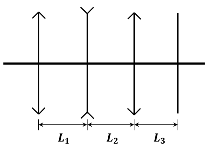
Figure 2: The OTE of JWST can be simplified to a set of lenses. The configuration comprises two convex lenses, positioned as the first and third lenses, with the second lens being concave and the fourth being flat.

We require that the light emitted from the primary mirror can reach the other three mirrors. For example, to check whether the light emitted from the primary mirror can reach the fine steering mirror, we use the following vector,

$$X=U_{3}U_{T}U_{2}U_{S}U_{1}X_{P}.$$ (31)

If the light can be received by the fine steering mirror, then the absolute value of the second component of vector $X$ has to be smaller than the radius of the fine steering mirror, which yields an inequality restricting the possible values of $y$. Therefore, by requiring that the light emitted by the primary mirror can be reflected three times and finally get into the detector, we have three inequalities which cut out an effective region on the surface of the primary mirror. Direct calculations show that this effective region is a rectangle with the length as 146.795 mm and the width as 104.248 mm. However, the primary mirror of JWST is hollowed in the center. The hollowed region is a hexagon with the side length as 762mm, which entirely encloses the effective region. Therefore, EM waves emitted by the primary mirror can’t be received by the detector.

We can perform a similar analysis for the the other three mirrors. The effective region is also rectangular, with the length and width as

$$a_{S}=132.904,\qquad b_{S}=94.3834.$$ (32)

The effective region of the tertiary mirror is rounded, with the diameter as

$$d_{T}=443.9$$ (33)

In addition, the whole area of the fine steering mirror is effective.

We also need to analyze the focusing ability. After a direct calculation, we find that

$$X_{S}\Rightarrow\begin{bmatrix}-0.00307001y\\ -6.20097y\end{bmatrix},\qquad X_{T}\Rightarrow\begin{bmatrix}-0.000331543y\\ -0.261223y\end{bmatrix},\qquad X_{F}\Rightarrow\begin{bmatrix}0\\ y\end{bmatrix}$$ (34)

where the unit of $y$ is millimeter. Let us take $X_{s}$ for example. After a series of reflections, the light emitted at the height $y$ goes into the detector at height $6.20097y$. This means that the energy emitted by a disk with radius $y$ is redistributed into a disk with radius $6.20097y$, and thus the energy flux density is $(6.20097)^{-2}$ the flux density emitted.

To sum up, the flux density inducedd by dark photon can be written as

$$I_{DM}=\frac{2}{3}\epsilon^{2}\rho_{\mathrm{DM}}\times(1+6.20097^{-2}+0.261223^{-2})$$ (35)

In order to compare our calculated result of the DPDM-induced EM signal with the real data recorded by JWST, we need to translate the induced signal into the equivalent flux density of the incoming astronomical EM signals. This means that we need to further calculate the focusing ability for the case of the incoming planar EM waves. The incoming plane waves can be described by a vector

$$X_{0}=\begin{bmatrix}0\\ y\end{bmatrix}.$$ (36)

We again use the transition matrices to calculate the light at the receiver,

$$X_{0}\Rightarrow\begin{bmatrix}7.52946\times 10^{-6}y\\ -0.0080392y\end{bmatrix}$$ (37)

Noting that the first entry is very small, we conclude that indeed the incoming planar wave is transformed into another planar wave. From the second entry, we get the enhancement factor $(0.0080392)^{-2}$. Thus, we can calculate the equivalent flux density by

$$I_{\mathrm{eqv}}\times(0.0080392)^{-2}=I_{DM}$$ (38)

which gives

$$I_{\mathrm{eqv}}=6.75618\times 10^{-4}\epsilon^{2}\rho_{\mathrm{DM}}.$$ (39)

However, there is one more subtlety. We have calculated the effective range of the secondary mirror and the tertiary mirror, the light emitted from the secondary mirror can indeed cover the whole receiver, but light emitted from the tertiary mirror is concentrated in a smaller region, and can only be observed with a well-chosen observation angle. To be very conservative, we simply assume that the light emitted by the tertiary mirror cannot go into the detector, and we have

$$I^{\prime}_{\mathrm{eqv}}=4.42064\times 10^{-5}\epsilon^{2}\rho_{\mathrm{DM}}.$$ (40)

V Constraints from JWST Observation Data

The James Webb Space Telescope (JWST) stands as the cutting-edge space telescope, equipped with various detectors and versatile observation modes. In our study, we harnessed data from 972 distinct observation projects to establish constraints on the Dark Photon-Dark Matter coupling constant. Out of these projects, 713 relied on the Near-Infrared Spectrograph (NIRSpec) [cite], while 259 made use of the Mid-Infrared Instrument (MIRI) [cite]. It is worth noting that the data selected for analysis excludes background subtraction, ensuring its suitability for our research.

The JWST data we collected from the Mikulski Archive for Space Telescopes (MAST) database MAS includes two crucial parameters: the measured spectral flux density, denoted as $\bar{O}_{i}$, and the associated statistical uncertainty, denoted as $\sigma_{\bar{O}_{i}}$. In our effort to establish upper limits on the coupling of Dark Photon with the Standard Model electromagnetic current, denoted as $\epsilon$, we followed the data analysis approach detailed in previous works Cowan et al. (2011); An et al. (2023c, a).

To provide a concise overview, we summarize the key aspects of our method here, while reserving more detailed information for Appendix A. Our analysis begins by applying a local polynomial function to model the background surrounding a selected frequency bin, $i_{0}$, while considering neighboring bins. We estimate systematic uncertainties by comparing data deviations to the background fit. Next, we introduce a hypothetical Dark Photon Dark Matter signal with a strength denoted as $S$ at the specific bin, $i_{0}$. This allows us to construct a likelihood function, $L$, that incorporates $S$ into the comparison between data and the background function. Nuisance parameters are introduced to account for the coefficients of the background polynomial function.

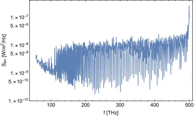
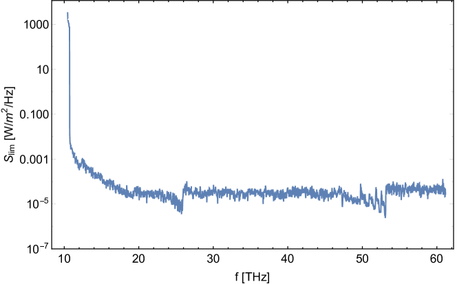
Figure 3: Model-independent 95% C.L. upper limits on a constant monochromatic signal from JWST data. The first figure corresponds to NIRSpec observation data, and the lower one MIRI. It shows the strongest limit from the all projects at each frequency bin.

Following the statistical method developed in Ref. Cowan et al. (2011), we compute the ratio, $\lambda_{S}$, between the maximized likelihood under two conditions: first, when only the nuisance parameters are varied to maximize $L$ while keeping $S$ constant, and second, when both the nuisance parameters and $S$ are varied to maximize $L$. The test statistic, $-2\log(\lambda_{S})$, follows a half-$\chi^{2}$ distribution Cowan et al. (2011). This analysis allows us to derive the $95\%$ confidence level upper limit, $S_{\mathrm{lim}}$, for a constant monochromatic signal. The results are illustrated in Fig. 3.

We establish upper limits on the mixing parameter $\epsilon$ as $S_{\mathrm{lim}}=S^{\prime}_{\mathrm{eqv}}$, where $S^{\prime}_{\mathrm{eqv}}$ represents the signal strength from theoretical calculations for Dark Photon Dark Matter. Different datasets from NIRSpec and MIRI yield varying constraints on the signal strength coupling $\epsilon$, and we select the most stringent among them. The constraint on $\epsilon$ and its comparison with previous experiments are illustrated in Fig. 4.

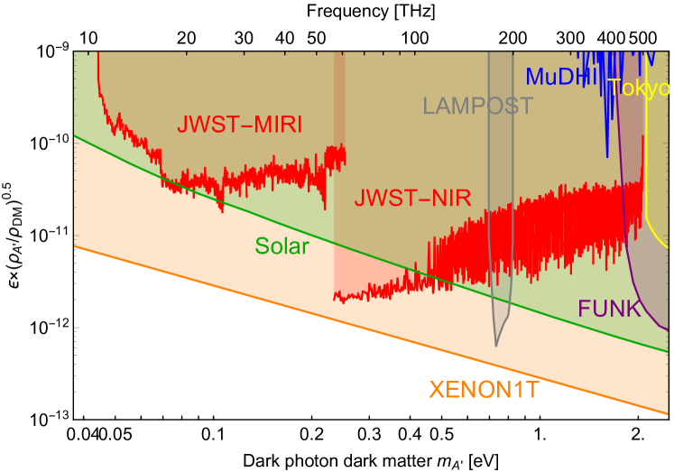
Figure 4: Constraints on the kinematic mixing parameter $\epsilon$ between Dark Photon Dark Matter (DPDM) and photons in the randomized polarization scheme. The solid red curve represents the $95\%$ confidence level (C.L.) exclusion limit for DPDM using JWST data. The left and right sections display constraints derived from NIRSpec and MIRI observation data, respectively. Additionally, we provide a comparison with existing limits, including those from Solar Li and Xu (2023), XENON1T Aprile et al. (2022), Lampost Chiles et al. (2022), Mudhi Manenti et al. (2022), Funk Andrianavalomahefa et al. (2020), and Tokyo Suzuki et al. (2015b).

VI Summary and Outlook

In this study, we conducted a direct detection search for dark photon dark matter (DPDM) using a haloscope setup. Our approach involved converting local DPDM into a normal electromagnetic field at the mirrors of the James Webb Space Telescope (JWST), which was then detected by its receiver. Due to the frequency match between the electromagnetic field and the DPDM mass, the resulting signal took the form of a monochromatic electromagnetic wave. Typically, accounting for the contribution of each surface area on the mirror to the electromagnetic field is necessary. The final electromagnetic energy received by the receiver encompasses the interference from each surface unit. We demonstrated that for high-mass DPDM, the contribution to the electromagnetic wave field at a given position primarily stems from the surface unit perpendicular to the separation vector, allowing us to calculate the electromagnetic flux at the receiver using ray-optics.

We utilized data from JWST observations to search for a monochromatic signal within the continuous background in the 10-500 terahertz (THz) range. Both the JWST Mid-Infrared Instrument (MIRI) and Near Infrared Spectrograph (NIRSpec) data were employed. Our analysis enabled us to establish limits on the DPDM kinetic mixing coupling at approximately $\epsilon\sim 3\times 10^{-11}$ and $\epsilon\sim\mathcal{O}(10^{-12})$ respectively. This broadband search for DPDM yielded valuable lower-frequency constraints, complementing other experiments conducted in room-sized laboratories, such as Lampost, Mudhi, FUNK, and TOKYO. However, our results indicated a coupling weaker by about one order of magnitude compared to the XENON1T results, which utilized the potential dark photon flux generated by the Sun, without assuming that the dark photon is the dark matter. Our results are also comparable with the astrophysical bound from the solar emission of the dark photon particles.

While our results are slightly weaker than XENON1T constraints, there exists potential for improvement given that JWST is not specifically designed for the direct detection of DPDM. JWST boasts an outstanding receiver capable of detecting THz signals. By incorporating a spherical mirror as the reflector, as proposed in Refs. Horns et al. (2013); Jaeckel and Redondo (2013b); Jaeckel and Knirck (2016), or adopting a flat reflector along with a parabolic collection mirror, akin to the design in the TOKYO experiment Knirck et al. (2018); Tomita et al. (2020) and the BRASS-p experiment Bajjali et al. (2023), it is possible to enhance sensitivity by orders of magnitude due to the right focus on the DPDM signal.

Appendix A Detailed derivation of Eq. (21)

Starting from equation (II.2), the integration over $\bm{k}^{\prime}$ can be done analytically,

$$\int_{<k_{\mathrm{esc}}} \frac{\mathrm{d}^{3}\bm{k}^{\prime}}{(2\pi)^{3}}e^{-\frac{2\bm{k}^{\prime 2}}{k_{0}^{2}}}e^{i\bm{k}^{\prime}\cdot(\bm{r^{\prime}}-\bm{r^{\prime\prime}})}=$$

$$\frac{k_{0}^{2}e^{-2z^{2}}e^{-iyz}}{32\sqrt{2}\pi^{2}\Delta r}\left[2\sqrt{2}i(-1+e^{2iyz})+\sqrt{\pi}ye^{-(y-4iz)^{2}/8}\left(\mathrm{erf}\left(\frac{4z+iy}{2\sqrt{2}}\right)+\mathrm{erf}\left(\frac{4z-iy}{2\sqrt{2}}\right)\right)\right]$$ (41)

where $\Delta r=|\bm{r^{\prime}}-\bm{r^{\prime\prime}}|$, $z=k_{\mathrm{esc}}/k_{0}$, and $y=k_{0}\Delta r$. When $z$ or $k_{\mathrm{esc}}$ is large, the expression above can be expanded as

$$\int_{<k_{\mathrm{esc}}}\frac{\mathrm{d}^{3}\bm{k}^{\prime}}{(2\pi)^{3}}e^{-\frac{2\bm{k}^{\prime 2}}{k_{0}^{2}}}e^{i\bm{k}^{\prime}\cdot(\bm{r^{\prime}}-\bm{r^{\prime\prime}})}\approx\frac{k_{0}^{3}}{16\sqrt{2}\pi^{3/2}}\left(e^{-\frac{1}{8}y^{2}}-\frac{2\sqrt{2}}{\sqrt{\pi}y}e^{-2z^{2}}\sin(yz)\right).$$ (42)

The next-to-leading order term is suppressed by $e^{-2z^{2}}$, and can be neglected. In addition, note that that

$$\rho_{\mathrm{DM}}=\frac{1}{2}\langle\bm{E^{\prime}}(\bm{r},t)\bm{E^{\prime}}^{*}(\bm{r},t)\rangle=\frac{ab^{2}}{64\pi^{2}}k_{0}^{3}|\bm{E^{\prime}}_{0}|^{2}\left(\sqrt{2\pi}\mathrm{erf}(\sqrt{2}z)-4ze^{-2z^{2}}\right)$$ (43)

which, under the large $z$ approximation, becomes

$$\rho_{\mathrm{DM}}=\frac{ab^{2}}{32\sqrt{2}\pi^{3/2}}k_{0}^{3}|\bm{E^{\prime}}_{0}|^{2}.$$ (44)

So the expression for $\langle\bm{S}\rangle_{t}$ reads

$$\langle\bm{S}\rangle_{t}=\rho_{\mathrm{DM}}\left(\frac{\epsilon}{\lambda}\right)^{2}\int\mathrm{d}S^{\prime}\mathrm{d}S^{\prime\prime}\left\{\left[\bm{\tau}(\bm{r^{\prime}})\times(\bm{r}-\bm{r^{\prime}})\right]\times(\bm{r}-\bm{r^{\prime}})\right\}\times[\bm{\tau}(\bm{r^{\prime\prime}})\times(\bm{r}-\bm{r^{\prime\prime}})]$$

$$\times e^{-\frac{1}{8}k_{0}^{2}|\bm{r^{\prime}}-\bm{r^{\prime\prime}}|^{2}}\mathrm{Re}\left(\frac{e^{im_{A^{\prime}}(|\bm{r}-\bm{r^{\prime}}|-|\bm{r}-\bm{r^{\prime\prime}}|)}}{|\bm{r}-\bm{r^{\prime}}|^{3}|\bm{r}-\bm{r^{\prime\prime}}|^{2}}\right)$$ (45)

Appendix B A Brief Proof of Eq. (8)

We demonstrate the one-dimensional case; extending to higher dimensions is straightforward.

We wish to evaluate

$$\lim_{\alpha\rightarrow\infty}\sqrt{\alpha}\int_{-\infty}^{\infty}g(x)e^{i\alpha f(x)}\mathrm{d}x$$ (46)

in the large $\alpha$ limit. In this analysis, we assume that $f(x)$ is second order differentiable, $g(x)$ is continuous. We also assume that $g(x)$ is either compactly supported or exhibits exponential decay and that $f^{\prime}(x)=0$ has only a discrete set of solutions. Here, we will focus on proving the case where $g(x)$ is compactly supported, noting that a similar approach can be applied when $g(x)$ has exponential decay.

Denote by $\Sigma$ the set of points where $f^{\prime}(x)=0$. Define

$$\Delta=\min\{x_{i}-x_{j}|x_{i},x_{j}\in\Sigma\}$$ (47)

Denote by $I$ the set on which $g(x)$ is supported. Define a set $A$ as follows,

$$A=\left\{[a,b]\left|[a,b]=\left[x_{0}-\frac{\delta}{2},x_{0}+\frac{\delta}{2}\right]\cap I\right.,\ x_{0}\in\Sigma\right\}$$ (48)

where $\delta$ is a positive real number that satisfies $\delta<\min\{\Delta,\alpha^{-1/2+\epsilon}\}$, with $\epsilon$ being a real number in the range $0<\epsilon<1/8$. Due to the continuity of $f^{\prime}(x)$, it follows that $f(x)$ is monotonic between any two adjacent points in $\Sigma$. Consequently, we can divide the interval $I$ into a finite set of closed intervals, each of which is either an element of $A$ or an interval on which $f(x)$ is strictly monotonic.

Let’s begin by examining the integral over intervals where $f(x)$ is monotonic.

$$\sqrt{\alpha}\int_{c}^{d}g(x)e^{i\alpha f(x)}\mathrm{d}x$$ (49)

Where $c$ and $d$ are two real numbers. Since $f(x)$ is monotonic, it has an inverse, here denoted by $f^{-1}(x)$. We define $y=f^{-1}(x)$, and the integral can be expressed as

$$\sqrt{\alpha}\int_{c^{\prime}}^{d^{\prime}}\tilde{g}(y)e^{i\alpha y}\mathrm{d}y$$ (50)

where $c^{\prime}=f(c)$, $d^{\prime}=f(d)$, and $\tilde{g}(y)=g(f^{-1}(y))(f^{-1})^{\prime}(y)$. It can be shown that this expression goes to zero as $\alpha\rightarrow\infty$. By dividing the interval $[c^{\prime},d^{\prime}]$ into a set of intervals with length $2\pi/\alpha$, integrating on each small interval contributes a result of order $\mathcal{O}(\alpha^{-3/2})$. Summing over all intervals gives an additional factor of $\alpha$, resulting in the overall order $\mathcal{O}(\alpha^{-1/2})$. Consequently, (50) vanishes in the large $\alpha$ limit.

Next consider the integral on elements of $A$:

$$\sqrt{\alpha}\int_{x_{0}-a}^{x_{0}+b}g(x)e^{i\alpha f(x)}\mathrm{d}x$$ (51)

where $x_{0}\in\Sigma$ and $\delta\geq a,\ b\geq 0$. Notice that

$$\sqrt{\alpha}\left|\int_{x_{0}-a}^{x_{0}+b}(g(x)-g(x_{0}))e^{i\alpha f(x)}\mathrm{d}x\right|\leq\sqrt{\alpha}(a+b)\sup_{x_{0}-a\leq x\leq x_{0}+b}\{g(x)-g(x_{0})\}=\mathcal{O}(\alpha^{-1/2+2\epsilon})$$ (52)

As $\alpha$ approaches infinity, the expression above tends to zero. Therefore, the integral we aim to evaluate can be replaced by the following expression,

$$\sqrt{\alpha}\int_{x_{0}-a}^{x_{0}+b}g(x_{0})e^{i\alpha f(x)}\mathrm{d}x$$ (53)

In the vicinity of $x_{0}$, $f(x)$ can be Taylor-expanded as

$$f(x)=f(x_{0})+\frac{1}{2}f^{\prime\prime}(x_{0})(x-x_{0})^{2}+R_{2}(x)$$ (54)

where $R_{2}(x)$ represents the remainder term. Divide the integral into two parts

$$\sqrt{\alpha}\int_{x_{0}-a}^{x_{0}+b} g(x_{0})e^{i\alpha f(x)}\mathrm{d}x=\sqrt{\alpha}\int_{x_{0}-a}^{x_{0}+b}g(x_{0})\exp\left[i\alpha\left(f(x_{0})+\frac{1}{2}f^{\prime\prime}(x_{0})(x-x_{0})^{2}\right)\right]\mathrm{d}x$$

$$+\sqrt{\alpha}\int_{x_{0}-a}^{x_{0}+b}g(x_{0})[\exp(i\alpha R_{2}(x))-1]\exp\left[i\alpha\left(f(x_{0})+\frac{1}{2}f^{\prime\prime}(x_{0})(x-x_{0})^{2}\right)\right]\mathrm{d}x$$ (55)

As $\alpha R_{2}(x)=\mathcal{O}(\alpha^{-1/2+3\epsilon})$, the second term is of order $\mathcal{O}(\alpha^{-1/2+4\epsilon})$, and therefore vanishes in the large $\alpha$ limit. Furthermore, in the large $\alpha$ limit, it can be demonstrated that the first term is equal to

$$\sqrt{\alpha}\int_{-\infty}^{\infty}g(x_{0})\exp\left[i\alpha\left(f(x_{0})+\frac{1}{2}f^{\prime\prime}(x_{0})(x-x_{0})^{2}\right)\right]\mathrm{d}x$$ (56)

We just have to prove that both

$$\sqrt{\alpha}\int_{-\infty}^{x_{0}-a}g(x_{0})\exp\left[i\alpha\left(f(x_{0})+\frac{1}{2}f^{\prime\prime}(x_{0})(x-x_{0})^{2}\right)\right]\mathrm{d}x$$ (57)

and

$$\sqrt{\alpha}\int_{x_{0}+b}^{\infty}g(x_{0})\exp\left[i\alpha\left(f(x_{0})+\frac{1}{2}f^{\prime\prime}(x_{0})(x-x_{0})^{2}\right)\right]\mathrm{d}x$$ (58)

tends to zero as $\alpha\rightarrow\infty$. Take (58) for example. Let’s define $t=\alpha(x-x_{0})^{2}$, substitute $x$ with $t$, and (58) becomes

$$g(x_{0})e^{i\alpha f(x_{0})}\int_{\alpha b^{2}}^{\infty}\frac{1}{2\sqrt{t}}\exp\left[\frac{1}{2}if^{\prime\prime}(x_{0})t\right]\mathrm{d}t$$ (59)

When $\alpha$ is sufficiently large, we have $\alpha b^{2}=\alpha^{2\epsilon}$. Therefore, as $\alpha$ approaches infinity, (58) tends to zero.

To sum up, we have

$$\int_{-\infty}^{\infty}g(x)e^{i\alpha f(x)}\mathrm{d}x=\sum_{x_{0}\in\Sigma}\int_{-\infty}^{\infty}g(x_{0})\exp\left[i\alpha\left(f(x_{0})+\frac{1}{2}f^{\prime\prime}(x_{0})(x-x_{0})^{2}\right)\right]\mathrm{d}x$$ (60)

The integral on the right-hand side is nothing but a Gaussian integral, so the result is

$$\int_{-\infty}^{\infty}g(x)e^{i\alpha f(x)}\mathrm{d}x=\sum_{x_{0}\in\Sigma}\sqrt{\frac{2\pi}{\alpha}}|f^{\prime\prime}(x_{0})|^{-1/2}e^{\frac{i\pi}{4}\mathrm{sgn}(f^{\prime\prime}(x_{0}))}g(x_{0})e^{i\alpha f(x_{0})}$$ (61)

It is straight forward to generalize to higher dimensional case. We can use the same method to prove that

$$\int_{\mathbb{R}^{n}}g(\bm{x})e^{i\alpha f(\bm{x})}\mathrm{d}^{n}\bm{x}=\sum_{\bm{x}_{0}\in\Sigma}\int_{\mathbb{R}^{n}}g(\bm{x}_{0})\exp\left[i\alpha\left(f(\bm{x}_{0})+\frac{1}{2}(\bm{x}-\bm{x}_{0})^{T}\mathrm{Hess}(f(\bm{x}_{0}))(\bm{x}-\bm{x}_{0})\right)\right]\mathrm{d}^{n}\bm{x}$$ (62)

Here $\Sigma$ is defined to be the set of points where $\nabla f=0$, and the Hessian matrix is defined to be

$$\mathrm{Hess}(f(\bm{x}))=\begin{bmatrix}\dfrac{\partial^{2}f}{\partial x_{1}^{2}}&\dfrac{\partial^{2}f}{\partial x_{1}\partial x_{2}}&\cdots&\dfrac{\partial^{2}f}{\partial x_{1}\partial x_{n}}\\ \dfrac{\partial^{2}f}{\partial x_{2}\partial x_{1}}&\dfrac{\partial^{2}f}{\partial x_{2}^{2}}&\cdots&\dfrac{\partial^{2}f}{\partial x_{2}\partial x_{n}}\\ \vdots&\vdots&\ddots&\vdots&\\ \dfrac{\partial^{2}f}{\partial x_{n}\partial x_{1}}&\dfrac{\partial^{2}f}{\partial x_{n}\partial x_{2}}&\cdots&\dfrac{\partial^{2}f}{\partial x_{n}^{2}}\end{bmatrix}$$ (63)

To evaluate the multidimensional Gaussian integral, we diagonalize the Hessian matrix. This transforms the integral into the product of $n$ one dimensional Gaussian integrals, ultimately leading to equation (8).

Appendix C Ray Transfer Matrix Analysis

In systems satisfying paraxial condition, we can utilize ”ray transfer matrix analysis” to simplify the calculations. A beam of light can be characterized by two parameters: the angle(counterclockwise) between the light and the optical axis, and the vertical distance(upward) between the light and the optical axis. These two parameters can be organized into a column vector

$$\bm{v}=\begin{bmatrix}\theta\\ y\end{bmatrix}$$ (64)

Here we assume that the light is travelling from left to right.

We can perform various operations on the light. First, it can travel a distance $L$ through free space, as depicted in Figure 5. During free travel, the angle $\theta$ remains unchanged, while the height $y$ increases by $\theta L$. This process can be described by the left multiplication of a matrix

$$\bm{v}\Rightarrow\bm{v}^{\prime}=\begin{bmatrix}1&0\\ L&1\end{bmatrix}\bm{v}$$ (65)

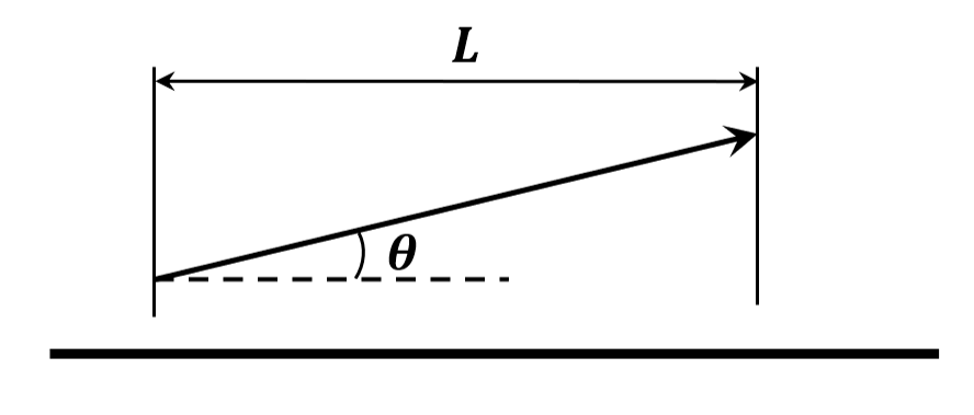
Figure 5: A beam of light travelling in free space

We can also represent the effects of reflectors using matrices. Reflecting changes the direction of the light from right-going to left-going, which can introduce complications. To simplify matters, we reflect the direction of the light, ensuring that it always travels rightward, as shown in figure 6.

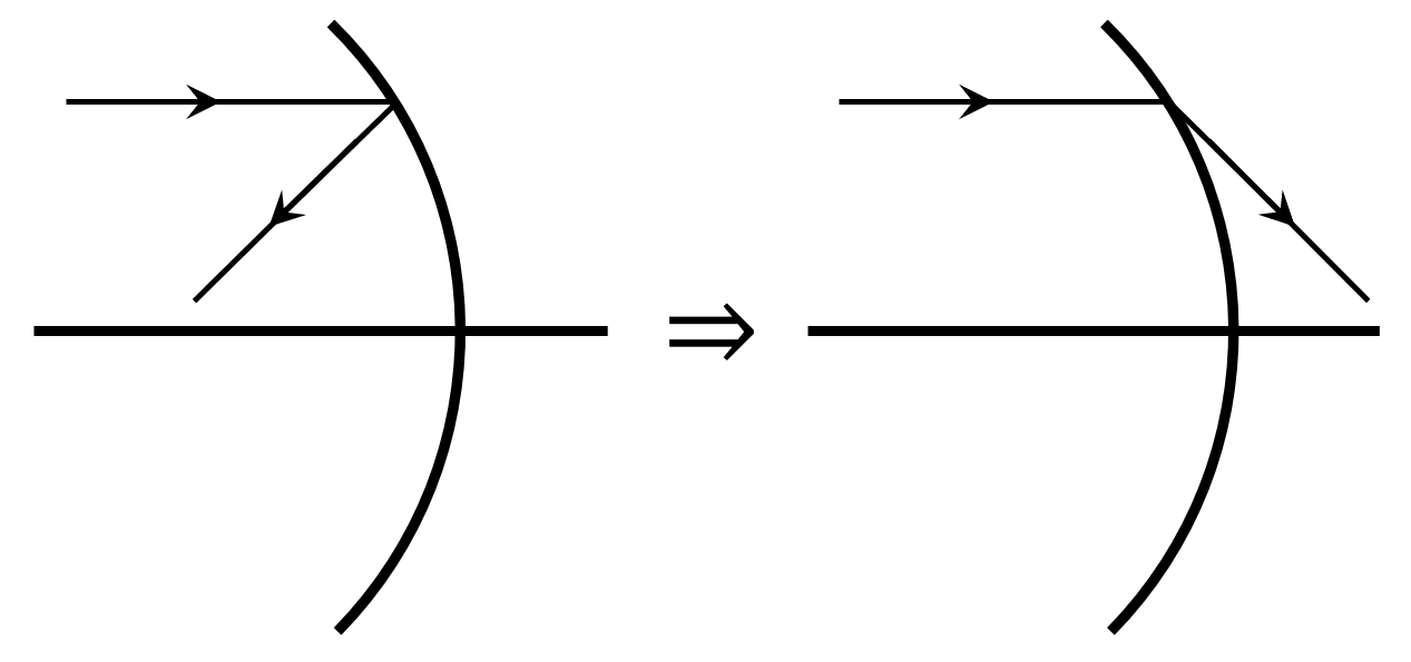
Figure 6: Reflecting the light so that it is always right-going

We are now prepared to analyze the effect of a reflector. When a beam of light is reflected by the reflector, its height remains unchanged while the direction $\theta$ is altered. Given that the paraxial condition is met, the reflector can be approximated by a spherical mirror, with its radius equal to the radius of curvature. Through direct analysis, we find that the effect of a reflector can be described by the following matrices

$$\begin{bmatrix}1&-\frac{2}{\rho}\\ 0&1\end{bmatrix}\mbox{(concave)}\qquad\begin{bmatrix}1&\frac{2}{\rho}\\ 0&1\end{bmatrix}\mbox{(convex)}$$ (66)

In the JWST setup, the axis of symmetry of the reflectors may differ from the optical axis, as shown in Figure 7 and Figure 8. Fortunately, the system is linear, so both of these effects simply add an overall constant to the beams of light we are considering.

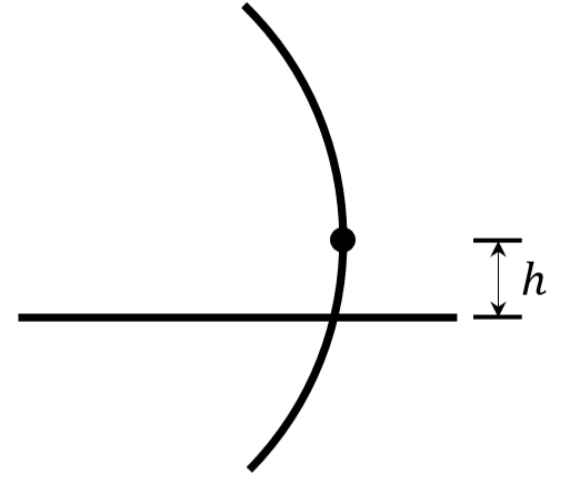
Figure 7: The center of the reflector is higher than the optical axis.

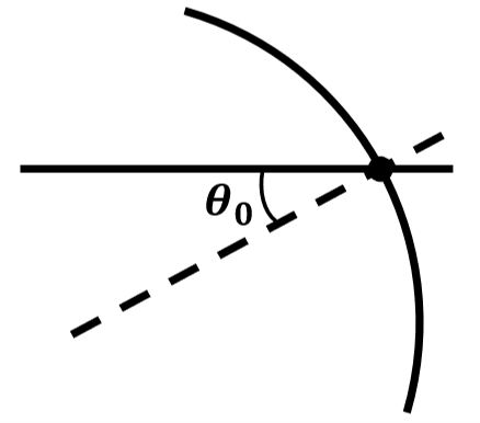
Figure 8: The axis of symmetry is not parallel to the optical axis.

First, if the center of the mirror is higher than the optical axis, the effect of the mirror is

$$\begin{bmatrix}\theta\\ y\end{bmatrix}\Rightarrow\begin{bmatrix}\theta-\frac{2y}{\rho}+\frac{2h}{\rho}\\ y\end{bmatrix}$$ (67)

So there is an overall angle $2h/\rho$, which can only cause overall vertical or angular displacement.

In the second case, where the axis of symmetry is not parallel to the optical axis, we have

$$\begin{bmatrix}\theta\\ y\end{bmatrix}\Rightarrow\begin{bmatrix}\theta-\frac{2y}{\rho}-2\theta_{0}\\ y\end{bmatrix}$$ (68)

Similarly, the $2\theta_{0}$ term can only cause overall vertical or angular displacements. As a result, the displacement of mirrors has no effect on the signal strength, allowing us to disregard the displacements and permitting light to pass through some mirrors if necessary.

Appendix D Data Analysis Method

The data analysis method adopted in the present work follows that in Cowan et al. (2011); An et al. (2023c, a). Utilizing JWST observation MAS , we have a dataset of spectral flux density $\bar{O}_{i}$ (mean value) along with the associated statistical error $\sigma_{\bar{O}_{i}}$ at a series of frequency bins indexed by $i$. To model the local flux background around bin $i_{0}$, We apply a polynomial function $B(a,f)$, fitting the data from bin $i_{0}-k$ to bin $i_{0}+k$,

$$B(a,f)=a_{0}+a_{1}f+a_{2}f^{2}+...+a_{n}f^{n}.$$ (69)

$a=\{a_{0},a_{1},a_{2},...,a_{n}\}$ are the coefficients of the polynomial terms. The weighted sum of squared residuals,

$$\sum_{i=i_{0}-k}^{i_{0}+k}\frac{1}{\sigma_{\bar{O}_{i}}^{2}}[B(a,f_{i})-\bar{O}_{i}]^{2},$$ (70)

is minimized at $a=\tilde{a}$. The deviations of the data points from the background fitting result, $\delta_{i}\equiv B(\tilde{a},f_{i})-\bar{O}_{i}$, can be modeled as a systematic error at bin $i_{0}$, that is

$$\sigma_{i_{0}}^{\rm sys}=\sqrt{\frac{1}{2k-1}\sum_{i=i_{0}-k}^{i_{0}+k}(\delta_{i}-\bar{\delta})^{2}}.$$ (71)

$\bar{\delta}$ is the average of the list $\delta_{i}$. Note that in computing Eqs. (70)-(71), we do not include the bin $i_{0}$ in the calculations. Additionally, for practical purposes, we set $n=3$ and $k=5$. By adding these two kinds of uncertainties in quadrature, we get the total uncertainty at bin $i_{0}$,

$$\sigma_{i_{0}}^{\rm sys}=\sqrt{(\sigma_{i_{0}}^{\rm sys})^{2}+\sigma_{\bar{O}_{i0}}^{2}}.$$ (72)

Next, to set upper limits on the coupling of DPDM with photon, we employ a likelihood-based statistical method Cowan et al. (2011). A likelihood function is constructed around bin $i_{0}$ as follows,

$$L(S,a)=\prod_{i=i_{0}-k}^{i_{0}+k}\frac{1}{\sqrt{2\pi}\sigma_{i}^{\rm tot}}\exp\left[-\frac{1}{2}\left(\frac{B(a,f_{i})+S\delta_{ii_{0}}-\bar{O}_{i}}{\sigma_{i}^{\rm tot}}\right)^{2}\right].$$ (73)

Here, we consider the parameter $a$’s as nuisance parameters. $S$ represents the DPDM-induced signal, and we assume its location to be in bin $i_{0}$. It’s worth noting that the frequency dispersion of DPDM is $\mathcal{B_{\rm DPDM}}\sim 0.15{\leavevmode\nobreak\ \rm kHz}\times(m_{A^{\prime}}/\mu{\rm eV})$. This is much smaller than the instrumental spectral resolution which ranges from 10 GHz to 40 THz, depending on different observation modes Gardner et al. (2006), so the DPDM-induced signal can be safely confined within a single frequency bin.

Then, we build the test statistic as

$$q_{S}=\begin{cases}-2\ln\frac{L(S,\hat{\hat{a}})}{L(\hat{S},\hat{a})},&\hat{S}\leq S\\ 0,&\hat{S}>S\end{cases}.$$ (74)

$L$ is maximized at $a=\hat{a}$ and $S=\hat{S}$; it is conditionally maximized at $a=\hat{\hat{a}}$ for a fixed $S$. As has been demonstrated in Ref. Cowan et al. (2011), the test statistic $q_{S}$ satisfies the half-chi-squared distribution,

$$f(q_{S}|S)=\frac{1}{2}\delta(q_{S})+\frac{1}{2}\frac{1}{\sqrt{2\pi}}\frac{1}{\sqrt{q_{S}}}\exp(-q_{S}/2),$$ (75)

the cumulative distribution of which is labeled as $\Phi(\sqrt{q_{S}})$. Then, we define the p-value function as $p_{S}=[1-\Phi(\sqrt{q_{S}})]/[1-\Phi(\sqrt{q_{0}})]$ which measures the deviation of the assumed signal $S$ to the null $S=0$. We set $p_{S}=5\%$ and then determine the value of $S$ corresponding to this $p_{S}$, which we denote as $S_{\rm lim}$. Consequently, if an assumed signal has a strength $S>S_{\rm lim}$, we can exclude it at the $95\%$ confidence level.

References

- Holdom (1986) Bob Holdom, “Two U(1)’s and Epsilon Charge Shifts,” Phys. Lett. 166B, 196–198 (1986).
- Dienes et al. (1997) Keith R. Dienes, Christopher F. Kolda, and John March-Russell, “Kinetic mixing and the supersymmetric gauge hierarchy,” Nucl. Phys. B 492, 104–118 (1997), arXiv:hep-ph/9610479 .
- Abel and Schofield (2004) S. A. Abel and B. W. Schofield, “Brane anti-brane kinetic mixing, millicharged particles and SUSY breaking,” Nucl. Phys. B 685, 150–170 (2004), arXiv:hep-th/0311051 .
- Abel et al. (2008a) S. A. Abel, M. D. Goodsell, J. Jaeckel, V. V. Khoze, and A. Ringwald, “Kinetic Mixing of the Photon with Hidden U(1)s in String Phenomenology,” JHEP 07, 124 (2008a), arXiv:0803.1449 [hep-ph] .
- Abel et al. (2008b) Steven A. Abel, Joerg Jaeckel, Valentin V. Khoze, and Andreas Ringwald, “Illuminating the Hidden Sector of String Theory by Shining Light through a Magnetic Field,” Phys. Lett. B 666, 66–70 (2008b), arXiv:hep-ph/0608248 .
- Goodsell et al. (2009) Mark Goodsell, Joerg Jaeckel, Javier Redondo, and Andreas Ringwald, “Naturally Light Hidden Photons in LARGE Volume String Compactifications,” JHEP 11, 027 (2009), arXiv:0909.0515 [hep-ph] .
- Redondo and Postma (2009) Javier Redondo and Marieke Postma, “Massive hidden photons as lukewarm dark matter,” JCAP 02, 005 (2009), arXiv:0811.0326 [hep-ph] .
- Nelson and Scholtz (2011) Ann E. Nelson and Jakub Scholtz, “Dark Light, Dark Matter and the Misalignment Mechanism,” Phys. Rev. D84, 103501 (2011), arXiv:1105.2812 [hep-ph] .
- Arias et al. (2012) Paola Arias, Davide Cadamuro, Mark Goodsell, Joerg Jaeckel, Javier Redondo, and Andreas Ringwald, “WISPy Cold Dark Matter,” JCAP 1206, 013 (2012), arXiv:1201.5902 [hep-ph] .
- Graham et al. (2016) Peter W. Graham, Jeremy Mardon, and Surjeet Rajendran, “Vector Dark Matter from Inflationary Fluctuations,” Phys. Rev. D93, 103520 (2016), arXiv:1504.02102 [hep-ph] .
- Alonso-Álvarez et al. (2019) Gonzalo Alonso-Álvarez, Thomas Hugle, and Joerg Jaeckel, “Misalignment & Co.: (Pseudo-)scalar and vector dark matter with curvature couplings,” (2019), arXiv:1905.09836 [hep-ph] .
- Nakayama (2019) Kazunori Nakayama, “Vector Coherent Oscillation Dark Matter,” JCAP 1910, 019 (2019), arXiv:1907.06243 [hep-ph] .
- Nakayama (2020) Kazunori Nakayama, “Constraint on Vector Coherent Oscillation Dark Matter with Kinetic Function,” JCAP 08, 033 (2020), arXiv:2004.10036 [hep-ph] .
- Ema et al. (2019) Yohei Ema, Kazunori Nakayama, and Yong Tang, “Production of Purely Gravitational Dark Matter: The Case of Fermion and Vector Boson,” JHEP 07, 060 (2019), arXiv:1903.10973 [hep-ph] .
- Kolb and Long (2021) Edward W. Kolb and Andrew J. Long, “Completely dark photons from gravitational particle production during the inflationary era,” JHEP 03, 283 (2021), arXiv:2009.03828 [astro-ph.CO] .
- Salehian et al. (2021) Borna Salehian, Mohammad Ali Gorji, Hassan Firouzjahi, and Shinji Mukohyama, “Vector dark matter production from inflation with symmetry breaking,” Phys. Rev. D 103, 063526 (2021), arXiv:2010.04491 [hep-ph] .
- Ahmed et al. (2020) Aqeel Ahmed, Bohdan Grzadkowski, and Anna Socha, “Gravitational production of vector dark matter,” JHEP 08, 059 (2020), arXiv:2005.01766 [hep-ph] .
- Nakai et al. (2020) Yuichiro Nakai, Ryo Namba, and Ziwei Wang, “Light Dark Photon Dark Matter from Inflation,” JHEP 12, 170 (2020), arXiv:2004.10743 [hep-ph] .
- Nakayama and Tang (2020) Kazunori Nakayama and Yong Tang, “Gravitational Production of Hidden Photon Dark Matter in Light of the XENON1T Excess,” Phys. Lett. B 811, 135977 (2020), arXiv:2006.13159 [hep-ph] .
- Firouzjahi et al. (2021) Hassan Firouzjahi, Mohammad Ali Gorji, Shinji Mukohyama, and Borna Salehian, “Dark photon dark matter from charged inflaton,” JHEP 06, 050 (2021), arXiv:2011.06324 [hep-ph] .
- Bastero-Gil et al. (2022) Mar Bastero-Gil, Jose Santiago, Lorenzo Ubaldi, and Roberto Vega-Morales, “Dark photon dark matter from a rolling inflaton,” JCAP 02, 015 (2022), arXiv:2103.12145 [hep-ph] .
- Firouzjahi et al. (2022) Hassan Firouzjahi, Mohammad Ali Gorji, Shinji Mukohyama, and Alireza Talebian, “Dark matter from entropy perturbations in curved field space,” Phys. Rev. D 105, 043501 (2022), arXiv:2110.09538 [gr-qc] .
- Sato et al. (2022) Takanori Sato, Fuminobu Takahashi, and Masaki Yamada, “Gravitational production of dark photon dark matter with mass generated by the Higgs mechanism,” (2022), arXiv:2204.11896 [hep-ph] .
- Co et al. (2018) Raymond T. Co, Aaron Pierce, Zhengkang Zhang, and Yue Zhao, “Dark Photon Dark Matter Produced by Axion Oscillations,” (2018), arXiv:1810.07196 [hep-ph] .
- Dror et al. (2018) Jeff A. Dror, Keisuke Harigaya, and Vijay Narayan, “Parametric Resonance Production of Ultralight Vector Dark Matter,” (2018), arXiv:1810.07195 [hep-ph] .
- Bastero-Gil et al. (2018) Mar Bastero-Gil, Jose Santiago, Lorenzo Ubaldi, and Roberto Vega-Morales, “Vector dark matter production at the end of inflation,” (2018), arXiv:1810.07208 [hep-ph] .
- Agrawal et al. (2018) Prateek Agrawal, Naoya Kitajima, Matthew Reece, Toyokazu Sekiguchi, and Fuminobu Takahashi, “Relic Abundance of Dark Photon Dark Matter,” (2018), arXiv:1810.07188 [hep-ph] .
- Co et al. (2021) Raymond T. Co, Keisuke Harigaya, and Aaron Pierce, “Gravitational waves and dark photon dark matter from axion rotations,” JHEP 12, 099 (2021), arXiv:2104.02077 [hep-ph] .
- Nakayama and Yin (2021) Kazunori Nakayama and Wen Yin, “Hidden photon and axion dark matter from symmetry breaking,” JHEP 10, 026 (2021), arXiv:2105.14549 [hep-ph] .
- Long and Wang (2019) Andrew J. Long and Lian-Tao Wang, “Dark Photon Dark Matter from a Network of Cosmic Strings,” (2019), arXiv:1901.03312 [hep-ph] .
- Fabbrichesi et al. (2020) Marco Fabbrichesi, Emidio Gabrielli, and Gaia Lanfranchi, “The Dark Photon,” (2020), 10.1007/978-3-030-62519-1, arXiv:2005.01515 [hep-ph] .
- Caputo et al. (2021) Andrea Caputo, Alexander J. Millar, Ciaran A. J. O’Hare, and Edoardo Vitagliano, “Dark photon limits: A handbook,” Phys. Rev. D 104, 095029 (2021), arXiv:2105.04565 [hep-ph] .
- De Panfilis et al. (1987) S. De Panfilis, A. C. Melissinos, B. E. Moskowitz, J. T. Rogers, Y. K. Semertzidis, Walter Wuensch, H. J. Halama, A. G. Prodell, W. B. Fowler, and F. A. Nezrick, “Limits on the Abundance and Coupling of Cosmic Axions at 4.5-Microev ¡ m(a) ¡ 5.0-Microev,” Phys. Rev. Lett. 59, 839 (1987).
- Wuensch et al. (1989) Walter Wuensch, S. De Panfilis-Wuensch, Y. K. Semertzidis, J. T. Rogers, A. C. Melissinos, H. J. Halama, B. E. Moskowitz, A. G. Prodell, W. B. Fowler, and F. A. Nezrick, “Results of a Laboratory Search for Cosmic Axions and Other Weakly Coupled Light Particles,” Phys. Rev. D40, 3153 (1989).
- Hagmann et al. (1990) C. Hagmann, P. Sikivie, N. S. Sullivan, and D. B. Tanner, “Results from a search for cosmic axions,” Phys. Rev. D42, 1297–1300 (1990).
- Asztalos et al. (2001) Stephen J. Asztalos et al. (ADMX), “Large scale microwave cavity search for dark matter axions,” Phys. Rev. D64, 092003 (2001).
- Asztalos et al. (2010) S. J. Asztalos et al. (ADMX), “A SQUID-based microwave cavity search for dark-matter axions,” Phys. Rev. Lett. 104, 041301 (2010), arXiv:0910.5914 [astro-ph.CO] .
- Hoang Nguyen et al. (2019) Le Hoang Nguyen, Andrei Lobanov, and Dieter Horns, “First results from the WISPDMX radio frequency cavity searches for hidden photon dark matter,” JCAP 1910, 014 (2019), arXiv:1907.12449 [hep-ex] .
- Horns et al. (2013) Dieter Horns, Joerg Jaeckel, Axel Lindner, Andrei Lobanov, Javier Redondo, and Andreas Ringwald, “Searching for WISPy Cold Dark Matter with a Dish Antenna,” JCAP 04, 016 (2013), arXiv:1212.2970 [hep-ph] .
- Jaeckel and Redondo (2013a) Joerg Jaeckel and Javier Redondo, “An antenna for directional detection of WISPy dark matter,” JCAP 11, 016 (2013a), arXiv:1307.7181 [hep-ph] .
- Jaeckel and Knirck (2016) Joerg Jaeckel and Stefan Knirck, “Directional Resolution of Dish Antenna Experiments to Search for WISPy Dark Matter,” JCAP 01, 005 (2016), arXiv:1509.00371 [hep-ph] .
- Knirck et al. (2018) Stefan Knirck, Takayuki Yamazaki, Yoshiki Okesaku, Shoji Asai, Toshitaka Idehara, and Toshiaki Inada, “First results from a hidden photon dark matter search in the meV sector using a plane-parabolic mirror system,” JCAP 1811, 031 (2018), arXiv:1806.05120 [hep-ex] .
- Gelmini et al. (2020) Graciela B. Gelmini, Alexander J. Millar, Volodymyr Takhistov, and Edoardo Vitagliano, “Probing dark photons with plasma haloscopes,” Phys. Rev. D 102, 043003 (2020), arXiv:2006.06836 [hep-ph] .
- McDermott and Witte (2020) Samuel D. McDermott and Samuel J. Witte, “Cosmological evolution of light dark photon dark matter,” Phys. Rev. D101, 063030 (2020), arXiv:1911.05086 [hep-ph] .
- An et al. (2021) Haipeng An, Fa Peng Huang, Jia Liu, and Wei Xue, “Radio-frequency Dark Photon Dark Matter across the Sun,” Phys. Rev. Lett. 126, 181102 (2021), arXiv:2010.15836 [hep-ph] .
- An et al. (2023a) Haipeng An, Xingyao Chen, Shuailiang Ge, Jia Liu, and Yan Luo, “Searching for Ultralight Dark Matter Conversion in Solar Corona using LOFAR Data,” (2023a), arXiv:2301.03622 [hep-ph] .
- An et al. (2023b) Haipeng An, Shuailiang Ge, and Jia Liu, “Solar Radio Emissions and Ultralight Dark Matter,” Universe 9, 142 (2023b), arXiv:2304.01056 [hep-ph] .
- Jaeckel and Redondo (2013b) Joerg Jaeckel and Javier Redondo, “Resonant to broadband searches for cold dark matter consisting of weakly interacting slim particles,” Phys. Rev. D 88, 115002 (2013b), arXiv:1308.1103 [hep-ph] .
- Suzuki et al. (2015a) Jun’ya Suzuki, Yoshizumi Inoue, Tomoki Horie, and Makoto Minowa, “Hidden photon CDM search at Tokyo,” in 11th Patras Workshop on Axions, WIMPs and WISPs (2015) pp. 145–148, arXiv:1509.00785 [hep-ex] .
- Suzuki et al. (2015b) J. Suzuki, T. Horie, Y. Inoue, and M. Minowa, “Experimental Search for Hidden Photon CDM in the eV mass range with a Dish Antenna,” JCAP 09, 042 (2015b), arXiv:1504.00118 [hep-ex] .
- Tomita et al. (2020) Nozomu Tomita, Shugo Oguri, Yoshizumi Inoue, Makoto Minowa, Taketo Nagasaki, Jun’ya Suzuki, and Osamu Tajima, “Search for hidden-photon cold dark matter using a K-band cryogenic receiver,” JCAP 09, 012 (2020), arXiv:2006.02828 [hep-ex] .
- Godfrey et al. (2021) Benjamin Godfrey et al., “Search for dark photon dark matter: Dark E field radio pilot experiment,” Phys. Rev. D 104, 012013 (2021), arXiv:2101.02805 [physics.ins-det] .
- Brun et al. (2019) Pierre Brun, Laurent Chevalier, and Christophe Flouzat, “Direct Searches for Hidden-Photon Dark Matter with the SHUKET Experiment,” Phys. Rev. Lett. 122, 201801 (2019), arXiv:1905.05579 [hep-ex] .
- Andrianavalomahefa et al. (2020) A. Andrianavalomahefa et al. (FUNK Experiment), “Limits from the Funk Experiment on the Mixing Strength of Hidden-Photon Dark Matter in the Visible and Near-Ultraviolet Wavelength Range,” Phys. Rev. D 102, 042001 (2020), arXiv:2003.13144 [astro-ph.CO] .
- Bajjali et al. (2023) Fayez Bajjali et al., “First results from BRASS-p broadband searches for hidden photon dark matter,” JCAP 08, 077 (2023), arXiv:2306.05934 [hep-ex] .
- Gardner et al. (2006) Jonathan P. Gardner et al., “The James Webb Space Telescope,” Space Sci. Rev. 123, 485 (2006), arXiv:astro-ph/0606175 .
- An et al. (2023c) Haipeng An, Shuailiang Ge, Wen-Qing Guo, Xiaoyuan Huang, Jia Liu, and Zhiyao Lu, “Direct detection of dark photon dark matter using radio telescopes,” Phys. Rev. Lett. 130, 181001 (2023c).
- Bleistein and Handelsman (1986) N. Bleistein and R.A. Handelsman, Asymptotic Expansions of Integrals, Dover Books on Mathematics Series (Dover Publications, 1986).
- Drukier et al. (1986) A. K. Drukier, Katherine Freese, and D. N. Spergel, “Detecting Cold Dark Matter Candidates,” Phys. Rev. D 33, 3495–3508 (1986).
- Evans et al. (2019) N. Wyn Evans, Ciaran A. J. O’Hare, and Christopher McCabe, “Refinement of the standard halo model for dark matter searches in light of the Gaia Sausage,” Phys. Rev. D 99, 023012 (2019), arXiv:1810.11468 [astro-ph.GA] .
- Lightsey et al. (2012) Paul Lightsey, Charles Atkinson, Mark Clampin, and Lee Feinberg, “James webb space telescope: Large deployable cryogenic telescope in space,” Optical Engineering 51, 1003– (2012).
- Lightsey et al. (2014) Paul A. Lightsey, J. Scott Knight, and Gary Golnik, “Status of the optical performance for the James Webb Space Telescope,” in Space Telescopes and Instrumentation 2014: Optical, Infrared, and Millimeter Wave, Society of Photo-Optical Instrumentation Engineers (SPIE) Conference Series, Vol. 9143, edited by Jr. Oschmann, Jacobus M., Mark Clampin, Giovanni G. Fazio, and Howard A. MacEwen (2014) p. 914304.
- (63) MAST 2021, JWST Archive Manual, eds. R.A. Shaw, B. Cherinka, P. Forshay, J. Yoon (Baltimore: STScI).
- Cowan et al. (2011) Glen Cowan, Kyle Cranmer, Eilam Gross, and Ofer Vitells, “Asymptotic formulae for likelihood-based tests of new physics,” The European Physical Journal C 71 (2011), 10.1140/epjc/s10052-011-1554-0.
- Li and Xu (2023) Shao-Ping Li and Xun-Jie Xu, “Production rates of dark photons and in the sun and stellar cooling bounds,” (2023), arXiv:2304.12907 [hep-ph] .
- Aprile et al. (2022) E. Aprile et al. (XENON), “Emission of single and few electrons in XENON1T and limits on light dark matter,” Phys. Rev. D 106, 022001 (2022), arXiv:2112.12116 [hep-ex] .
- Chiles et al. (2022) Jeff Chiles et al., “New Constraints on Dark Photon Dark Matter with Superconducting Nanowire Detectors in an Optical Haloscope,” Phys. Rev. Lett. 128, 231802 (2022), arXiv:2110.01582 [hep-ex] .
- Manenti et al. (2022) Laura Manenti et al., “Search for dark photons using a multilayer dielectric haloscope equipped with a single-photon avalanche diode,” Phys. Rev. D 105, 052010 (2022), arXiv:2110.10497 [hep-ex] .