Integrated Interpolation and Block-term Tensor Decomposition for Spectrum Map Construction
Abstract
This paper addresses the challenge of reconstructing a 3D power spectrum map from sparse, scattered, and incomplete spectrum measurements. It proposes an integrated approach combining interpolation and block-term tensor decomposition (BTD). This approach leverages an interpolation model with the BTD structure to exploit the spatial correlation of power spectrum maps. Additionally, nuclear norm regularization is incorporated to effectively capture the low-rank characteristics. To implement this approach, a novel algorithm that combines alternating regression with singular value thresholding is developed. Analytical justification for the enhancement provided by the BTD structure in interpolating power spectrum maps is provided, yielding several important theoretical insights. The analysis explores the impact of the spectrum on the error in the proposed method and compares it to conventional local polynomial interpolation. Extensive numerical results demonstrate that the proposed method outperforms state-of-the-art methods in terms of signal source separation and power spectrum map construction, and remains stable under off-grid measurements and inhomogeneous measurement topologies.
Index Terms:
Integrated, interpolation, block-term tensor decomposition, alternating minimization, sparse observations, power spectrum map.I Introduction
Spectrum maps, or more specifically, power spectrum maps, enable various applications in wireless signal processing and communications, such as signal propagation modeling [1, 2], source localization [3, 4], wireless power transfer [5], and radio resource management [6]. It has been a challenging problem in constructing power spectrum maps. Firstly, measurement data is only available in a limited locations or along a few routes, but the spatial pattern of the power spectrum map can be very complex due to possible signal reflection and attenuation from the propagation environment. Second, the location and the power spectrum of the signal source can be time-varying, and therefore, the power spectrum map should be constructed within a limited time based on limited measurements.
There has been active research on power spectrum map construction. Traditional interpolation-based approaches construct each map point as a linear combination of nearby measurements, where the weights can be found using different methods including Kriging [7, 8], local polynomial regression [9], and kernel-based methods [10, 11]. Compressive sensing inspired approaches exploit the fact that the matrix representation of a power spectrum map has a low-rank structure, and thus, dictionary learning [12] and matrix or tensor completion [13, 14, 15, 6] can be applied to interpolate or extrapolate the power spectrum information at locations without measurements. Recent work [6] proposed an orthogonal matching pursuit using a tensor model for 3D spectrum mapping. The approach in [15] reconstructed the power spectrum map through minimizing the tensor rank while also enforcing smoothness. Deep learning-based approaches [16, 17] treated the power spectrum map as one or multiple layers of 2D images, and neural networks were trained to memorize the common pattern of these images based on a huge amount of training data.
Many of these approaches were originally developed by representing the power spectrum map as one or multiple 2D data layers, for example, each layer representing a 2D power spectrum map for a specific frequency band. Although most existing approaches can be directly extended to the case in a higher dimension, their construction performance substantially degrades due to the curse of dimensionality unless a special structure is utilized. To address this issue, recent studies proposed a block-term tensor decomposition (BTD) model to exploit the spatial correlation of the power spectrum map at different frequency bands [18, 19]. The BTD model captures the property that if a signal from a particular source in a certain frequency band is blocked at a specific location, it is likely that signals from the same source at different frequency bands will also be blocked at that location. In [18], a power spectrum map was reconstructed using a BTD model where power spectrum and spatial loss field were constructed separately. The method in [19] applies a deep neural network to the tensor decomposition model to learn the intricate underlying structures.
However, tensor decomposition for power spectrum map construction has several limitations. First, the assumption of low-rank properties in matrix or tensor models relies on on-grid measurements, a condition rarely met in reality due to physical constraints on sensor placements. Off-grid measurements induce discretization errors that likely destroy the low-rank property, and consequently, degrade the performance of matrix or tensor completion. Second, while one can reduce the grid size to reduce the discretization error, a small grid size will translate to a large matrix dimension, and this leads to the identifiability issue as the matrix or tensor can be too sparse to complete. To address the issue of off-grid measurements, recent works proposed to joint interpolation with matrix or tensor completion [20, 21]. The work [20] applied adaptive interpolation to estimate the values at the grid points, and then, performed uncertainty-aware matrix completion according to the estimated interpolation errors. In [21], thin plate spline (TPS) interpolation was used to construct each layer of the tensor, followed by BTD to construct the power spectrum map.
However, existing approaches [20, 21] are open loop approaches, where interpolation and tensor completion are sequentially performed for different objectives under different models; but a non-ideal interpolation may destroy the desired BTD structure. Our preliminary work [22] proposed a closed loop approach to integrate interpolation and tensor completion, where a tensor structure guided interpolation problem was formulated, but by how much the tensor structure may help the interpolation was not theoretically clear.
This paper aims to construct a 3D data array representing the spectrum information over a 2D area, based on sparse, scattered, and incomplete spectrum measurements. A tensor model is formed, where each slice of the tensor represents a power spectrum map of one frequency band. To integrate interpolation with tensor completion, we perform interpolation framed by the BTD tensor structure, and in addition, the interpolation is regularized by the low-rank property of the slices of the tensor. The BTD model captures the spatial correlation of the power spectrum maps across different frequency bands under the large-scale fading, and the small-scale frequency-selective fading is treated as noise that can be mitigated by the regression to the local polynomial interpolation model. The low-rank regularization is to enforce the interpolation to be aware of the global data structure. Analytical results are established to understand the gain for the interpolation under the BTD model. It is found that, at low signal-to-noise ratio (SNR), the power spectrum map excited by narrowband sources is easier to construct than the one excited by wideband sources, whereas, at high SNR, the one excited by a wideband source with a uniform spectrum is easier to construct. The reconstruction performance under overlapping spectrum for a two-source case is also analyzed. Our numerical experiments demonstrate that the proposed scheme works much better in separating two sources when they have overlapping spectrums as compared to state-of-the-art schemes, and the proposed algorithm is stable under off-grid measurements. An improvement of over % in reconstruction accuracy is observed, regardless of whether the sensors measure the full or sparse spectrum.
To summarize, the following contributions are made:
-
•
We propose an integrated interpolation and BTD approach for constructing power spectrum maps. The method incorporates an interpolation model with the BTD structure to exploit the spatial correlation of the power spectrum maps. A nuclear norm regularization is used to exploit the low-rank property of the power spectrum maps.
-
•
We develop an alternating regression and singular value thresholding algorithm for the integrated interpolation and BTD problem.
-
•
We establish analytical justification on why the BTD structure may enhance the interpolation for power spectrum map construction, with several important theoretical insights obtained from the analysis.
-
•
Extensive numerical studies are conducted and show that the proposed method surpasses existing methods in terms of signal source separation and power spectrum map construction, and it is stable under off-grid measurements and inhomogeneity of the measurement topology.
The rest of the paper is organized as follows. Section II establishes the signal model and tensor model. Section III develops an integrated interpolation and BTD approach with a matrix formulation of the proposed method is provided. An alternating regression and singular value thresholding algorithm is developed to solve the proposed method. Section IV theoretically analyzes the error of the proposed method and compares it with conventional local polynomial interpolation. It then numerically discusses low-rank regularization and the performance of signal source separation. Numerical results are presented in Section V and conclusion is given in Section VI.
Notation: Vectors are written as bold italic letters , matrices as bold capital italic letters , and tensors as bold calligraphic letters . For a matrix , denotes the entry in the th row and th column of . For a tensor , denotes the entry under the index . The symbol ‘’ represents outer product, ‘’ represents Kronecker product, and represents Frobenius norm. The notation means , represents a diagonal matrix whose diagonal elements are the entries of vector , and denotes the vectorization of matrix . The symbol and denote expectation and variance separately.
II System Model
II-A Signal Model
Consider that a bounded area contains signal sources. The signals occupying frequency bands are detected by sensors at known locations , . Denote as the location of the th source. Then, the signal power from the th signal source measured at the th frequency band and location is modeled as
| (1) |
where describes the path gain of the th source at distance , the function describes the distance between a source at and a sensor at , captures the shadowing of the signal from the th source, is a zero mean Gaussian random variable to model the fluctuation due to the frequency-selective fading, and describes the power allocation of the th source at the th frequency band. Note that the values of all these components are not known to the system.
The aggregated power at the th frequency band from all the sources measured by a sensor located at is denoted as
| (2) |
where is to model the measurement noise at each frequency band, and contains the set of frequency bands that are measured by the th sensor. We assume that for each source , the total power sums to , and therefore, the SNR is normalized to , where is the total noise for the entire bandwidth.
Consider to discretize the target area into rows and columns that results in grid cells. Let be the center location of the th grid cell. Our goal is to reconstruct the large-scale propagation field, i.e., the first two terms in (1)
| (3) |
at grid points and the power spectrum , . The reconstructed propagation field model (3) does not capture the frequency-selective fading .
II-B Tensor Model
Let be a discretized form of the propagation field for the th source, where the th entry is given by . It has been widely discussed in the literature that for many common propagation scenarios, the matrix tends to be low-rank [1, 18].
Let be a tensor representation of the target power spectrum maps to be constructed. Based on (1) and (3), we have to represent the aggregated power of the th frequency band from the sources measured at location exempted from the small-scale fading component . Denote as the power spectrum from the th source. As a result, the tensor has the following BTD structure
| (5) |
where ‘’ represents outer product.
Conventional tensor-based power spectrum map construction approaches obtain the complete tensor from the measurement assuming that are taken at the center of the grid cell without measurement noise [15, 6]. However, when the grid cells are too large, corresponding to small and , it is hard to guarantee that the sensor at is placed at the corresponding grid center , resulting in possibly large discretization error. When the grid cells are small, corresponding to large and , there might be an identifiability issue as the dimension of the tensor is large.
Recent attempts [20, 21, 23] consider to first estimate using interpolation methods based on the off-grid measurements, and then, employ matrix completion or tensor completion based on the BTD model (5) to improve the spectrum map construction. However, these methods are open-loop methods where the property that are low-rank matrices is not exploited in the interpolation step; consequently, a poor open-loop interpolation may affect the performance in the tensor completion step.
III Integrated Interpolation and BTD Approach
In this section, we propose an integrated interpolation and BTD approach, where the BTD structure of the tensor model and the low-rank property of the tensor components are both exploited for interpolation.
III-A The Integrated Interpolation and BTD Problem
Based on the BTD model in (5), we consider to fit a model to approximate the large-scale propagation field of the th source in (3) from the multi-band measurements by exploiting the structure of the tensor model and the low-rank property of the tensor component .
Here, we adopt a polynomial model for the propagation field of the th source, but note that, other conventional interpolation approaches, including Kriging and kernel regression, also work with the proposed framework. The global model for source can be constructed based on a number of local models on selected cells . Without loss of generality (w.l.o.g.), a second order polynomial model for the th grid cell centered at is given as follows:
| (6) |
We collect the model parameters of the local model at cell for the th source into a vector , and is a collection of model parameters at cell for all sources.
It follows that, under perfect interpolation that yields , we have , which aligns with the BTD tensor structure in (5). Therefore, a BTD tensor structure guided least-squares local polynomial regression based on the measurements at the location can be constructed through minimizing the following cost
| (7) |
The term is a kernel function with a parameter to weight the importance of the measurements. A possible choice of kernel function can be the Epanechnikov kernel [9].
In an extreme case, local interpolation can be performed individually for all cells where includes all entries, but the computation complexity can be very high when and are large. Therefore, we are interested in the case of interpolating only a few (sparsely) selected grid cells due the spatial correlation of the propagation field. As a result, the cost function for the global model can be written as follows:
| (8) |
The regression model (8) is not aware of the hidden low-rank property of the propagation filed. We thus propose an integrated interpolation and BTD formulation to impose the low-rank for the global model as follows:
| (9) |
where represents the nuclear norm. As a result, the regression model not only needs to fit the measurement data via minimizing the cost in (8) but is also penalized by the rank of via the second and the third terms in (9).
III-B Matrix Formulation of Integrated Interpolation and BTD
It turns out that the minimization problem (9) has a nice structure after reformulation with matrix representations.
Denote . Then, the polynomial model in (6) is rewritten as
Denote , and recall the definition of in (7). From (7), we have where ‘’ is the Kronecker product. The least-squares local polynomial regression model (7) is rewritten as follows:
| (10) |
where indicates the observation status of th frequency band at location , if , we have , elsewise . For the convenience of matrix form formulation, we denote .
Next, we further rearrange (10) into a matrix form. Denote . To concisely express the mathematical relationships, we first replace the summation term over in (10) with its matrix form as follows:
| (11) |
where , and respectively represent the th column of and . The matrix is an diagonal matrix with the th diagonal element equals to .
Further, based on (11), we replace the summation term over with its matrix form. Denote . Then, model (11) can be written as follows:
where is an diagonal matrix,
| (12) |
and is an identity matrix.
From (6), if , then we have , where is a unit vector with the th entry equals , and all the other elements equal . Thus, the integrated interpolation and BTD problem (9) can be rewritten as follows:
| subject to | (13) |
where is a collection of received signal strength (RSS) , is the power spectrum which is non-negative, is the diagonal matrix of weights defined in (12), is a collection of measurement locations , and is a discretized form of propagation field in (5).
III-C Alternating Regression and Singular Value Thresholding
It is observed in (13) that given the matrix components and the spectrum variable , the objective is a convex quadratic function in the regression parameters . Likewise, given and , (13) is also a convex quadratic function in ; and moreover, (13) is a convex function in . Therefore, it is natural to adopt an alternating optimization approach to solve for the integrated interpolation and BTD problem (13).
Update of : Given the values of and , the optimization problem (13) is equivalent to a weighted least-squares problem as follows:
| (14) |
Note that the problem (14) is an unconstrained strictly convex problem. Hence, the solution can be obtained through setting the first order derivative of (14) to zero and we get:
| (15) |
Update of : Similarly, given the values of and , the optimization problem (13) is equivalent to a constrained weighted least-squares as follows:
| subject to | (16) |
Using the property of Kronecker product and [24], problem (16) can be rewritten as:
| subject to | (17) |
where is the reformed matrix form of vector with dimension .
Note that the th grid in set is a one-to-one mapping to the th grid. Denote , and . We reformulate (17) to make it a general non-negative constrained least-squares problem as follows:
| subject to | (18) |
Note that the problem (18) is a strictly convex problem. Hence, it has a unique optimal solution and a single principal pivoting algorithm [25] can be applied to solve (18).
Update of : Finally, with the and updated through (15) and (18), the optimization problem (13) is equivalent to a nuclear norm regularized low-rank matrix completion problem as follows:
| (19) |
It is observed that (19) can be equivalently decomposed into parallel sub-problems each focusing on an as follows:
| (20) |
Denote the observation matrix as . Then, the singular value thresholding algorithm can be applied to solve (20) through the iteration as follows [26]:
| (21) |
where is an intermediate matrix, represents the index of each iteration, if and zero otherwise, and is the soft-thresholding operator which is defined as follows:
with , , , and is the singular value decomposition (SVD) of where is the rank of .
Each sub-problem of (13) is strictly convex and has a unique solution. Since the overall objective value decreases (or at least does not increase) with each iteration, and the objective (9) is lower bounded by , the alternating regression and singular value thresholding algorithm must converge.
Finally, the power spectrum map is constructed as .
IV Performance of the Integrated Interpolation and BTD Approach
This section investigates the performance and the potential advantage of the proposed integrated interpolation and BTD approach (9) from three aspects. First, we focus on the least-squares cost term by dropping the low-rank regularization in (9). By analyzing the interpolation error, we show that the proposed method indeed yields a better accuracy. Then, we numerically verify that by imposing the low-rank regularization, the reconstruction accuracy can be further improved. Finally, we discuss how the proposed structure may improve the identifiability of separating multiple sources compared to the classical tensor-based approaches.
IV-A Improvement from the BTD Model
We first show that exploiting the BTD model in (5) can increase the accuracy of constructing .
IV-A1 Single Source
Let us start from the case of full spectrum observation for a single source, where and each sensor measures all the frequency bands, i.e., in (11) is an all ’s matrix. The result can be easily extended to the case where each sensor only observes a subset of frequency bands.
For the sake of notation simplicity, we omit the superscript "(r)" and adopt symbols , , and so on, to represent , , and similar variables. Recall that is a model to approximate , and from (6). Define the interpolation error as where is an estimate of .
Assume that the propagation field in (1) is third-order differentiable. Then, if is available, we have the following results to characterize the construction error at a point of the integrated interpolation and BTD approach.
Theorem 1 (Full spectrum error analysis).
Proof.
See Appendix A. ∎
It is observed that the variance of the interpolation error depends on the spectrum of the source. An analysis of the coefficients is given in the following proposition.
Proposition 1 (Impact from the spectrum).
The coefficients in (22) satisfy
with lower bound achieved when and upper bound achieved when . In addition,
with lower bound achieved when and upper bound achieved when .
Proof.
See Appendix B. ∎
One can make the following observations. First, the impact from the frequency-selective fading due to the power allocation of the source is more significant than that from the measurement noise, in the sense that for , we have for all power spectrum . The intuition is that the frequency-selective fading component is multiplied with the power allocation in (1) for the contribution to the measurement in (4), and hence, a power boost in the th frequency band also enhances the frequency-selective fading component.
Second, it follows that equal-power allocation minimizes the impact of the frequency-selective fading under the integrated interpolation and BTD approach. In this case, the fading component can be treated as additional measurement noise, resulting in a combined noise with variance . The more frequency bands that can be measured, the less impact from the frequency-selective fading.
Third, on the contrary to the impact of the frequency-selective fading, the noise term prefers a power boost in just one frequency band. This is because reducing the bandwidth also reduces the noise power, resulting in an increase in the SNR.
To summarize, in the high SNR scenario, where the measurement noise power is much smaller than the amount of the frequency-selective fading , a wide-band measurement with equal power allocation is preferred for constructing the propagation map . On the contrary, in the low SNR scenario, a narrow-band measurement is preferred and all the power should be allocated to a single frequency band. This is mathematically summarized in the following corollary.
Corollary 1 (Asymptotic performance).
At high SNR, the uniform spectrum asymptotically minimizes as , and consequently, . At low SNR, the single band measurement under asymptotically minimizes as , and consequently, .
For performance bench-marking, we consider a conventional frequency-by-frequency construction for each , using a local polynomial interpolation technique under the same regression model (6). Specifically, for each , we construct only based on and the measurement of the th frequency band using local polynomial regression under the same parameter and the kernel function. Likewise, the spectrum is available. Denote as the estimated power spectrum at location .
Proposition 2 (Interpolation without a BTD model).
Let , and where . Under the same assumption as in Theorem 1, the variance of the interpolation error is given by
| (23) |
Proof.
See Appendix C. ∎
It is observed that the impact from the frequency-selective fading is independent of the spectrum , which is in contrast to (22) for the case with the tensor guidance. This is due to the fact that only the data for the same frequency band is used. The coefficient of measurement noise in (23) is lower bounded by with lower bound achieved when . Note that this error coefficient can be arbitrarily large for an arbitrarily small in a particular frequency band . On the contrary, the construction performance for the integrated interpolation and BTD approach in (22) is less affected even for some .
To make a more specific comparison, we derive the difference .
Proposition 3 (Interpolation error reduction).
Under the same assumption as in Theorem 1, the proposed integrated interpolation and BTD approach reduces the variance of the interpolation error by
| (24) |
where and
In addition, where the second and third inequalities are achieved when and the inequality in first inequality is achieved when .
Proof.
See Appendix D. ∎
It is observed that the integrated interpolation and BTD approach is always of smaller variance than the conventional frequency-by-frequency local polynomial interpolation. In addition, the error from the measurement noise is more significant than that from the frequency-selective fading, in the sense that for , we have , because .
Finally, we extend our discussion to the case of sparse spectrum observation. We assume each sensor randomly measures frequency bands. To simplify the discussion, we assume the source has equal power allocation over all frequency bands.
Proposition 4 (Sparse spectrum error analysis).
Under the same condition of Theorem 1, the variance of the interpolation error for the integrated interpolation and BTD approach is given by
Proof.
See Appendix E. ∎
Proposition 4 verifies that the interpolation performance for the integrated interpolation and BTD approach depends on the number of observed frequency bands in each sensor, rather than the measurement pattern in the frequency domain, i.e., different sensors can observe different subsets of frequency bands. For instance, we may have more measurements for some frequency bands, while other frequency bands have rare measurements, and such a heterogeneous situation does not affect the performance for the integrated interpolation and BTD approach.
IV-A2 Multiple Sources
We demonstrate the result for a two-source case, where the derivation for is straight-forward, and similar insights can be obtained.
Consider that the two sources occupy frequency bands. There are frequency bands that are occupied by both sources where is the overlapping ratio, and distinct frequency bands are occupied by each source separately. Assume equal power allocation across frequency bands for each source.
Since the configuration is symmetric, it suffices to analyze the reconstruction for the th source, , and we have , . Assume that the propagation field in (1) is third-order differentiable. Then, if is available, we have the following results to characterize the construction error at a point .
Theorem 2 (Spectrum overlap for multiple sources).
In addition, with lower bound achieved when .
Proof.
See Appendix F. ∎
It is found that when , i.e., there is no overlap of frequency bands between each source, we have the coefficients and to be , which is consistent with the results in Theorem 1 for a signal case, where each source occupies frequency bands. Increasing the overlapping ratio also increases the coefficients and in (25), leading to a worse performance. When reaches 1, we will mathematically have the matrix in (48) to be singular, and the estimation error can be arbitrarily large. In this case, one cannot separate the two sources.
IV-B Low-rank Regularization
The nuclear norm regularization in the third term of (9) provides two benefits: First, it allows sparse interpolation in the first term , where in (8) may only contain a small set of grids to interpolate, and second, it imposes low-rank of the propagation field represented by the matrix . Note that while the interpolation in (9) exploits the locally spatial correlation of the propagation field, the low-rank regularization tries to exploit the global structure, where the signal strength may decrease in all directions following roughly the same law as distance increases.
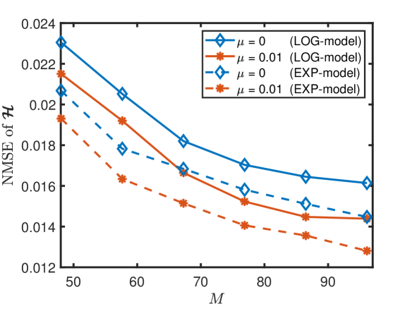
To numerically study the performance gain due to low-rank regularization, we select two common forms of propagation model. One is under exponential scale (EXP-model) , with , , another is under log-scale (LOG-model) , with , , , where represents the distance from the source at the origin, is the coordinate of the grid cell, and is the height. We choose the number of sources , dimension , the number of frequency bands , and the number of measurements with sampling rate . The performance criterion normalized mean squared error (NMSE) is the same as in Section V.
Fig. 1 compares two schemes, one with the low-rank regularization where in (19), and the other without the low-rank regularization where . We choose in (14) for both the two schemes. Fig. 1 shows that the low-rank regularization can enhance the accuracy in the reconstruction by more than % for both propagation models compared to the case without regularization under the sparse observations. It is observed that the proposed scheme with low-rank regularization outperforms a interpolation scheme without the low-rank regularization.
IV-C Identifiability of Multiple Sources with Overlapping Spectrum
One important feature of the proposed method is the capability of identifying multiple sources possibly with overlapping spectrum. This feature was also exploited by the related works based on tensor decomposition in the literature [18, 21]. However, the proposed scheme has the advantage that it does not require a priori knowledge of the rank of . By contrast, existing schemes based on the BTD model require the rank information as needs to be decomposed into [18, 21]. Estimating the rank parameter for the existing schemes can be challenging, because a small may lose some accuracy, whereas, a large may lead to identifiability issue.
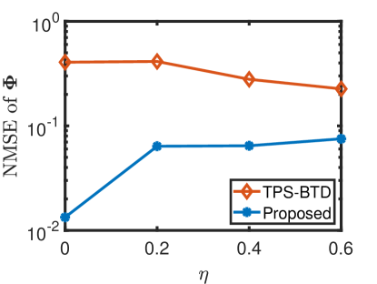
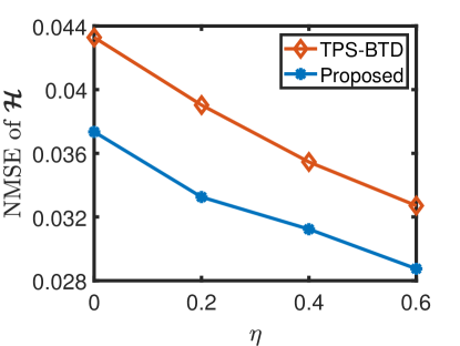
To numerically analyze the identifiability for multiple sources with overlapping spectrum, we choose the overlapping ratio , then, the number of overlapped frequency bands is with a total frequency bands observed of each source. We set , and then normalize for comparison. We choose , , , other settings are the same as in Section V. Since the TPS method reconstructs the whole tensor without separating the source, we only compare the proposed method with the TPS-BTD baseline in Section V.
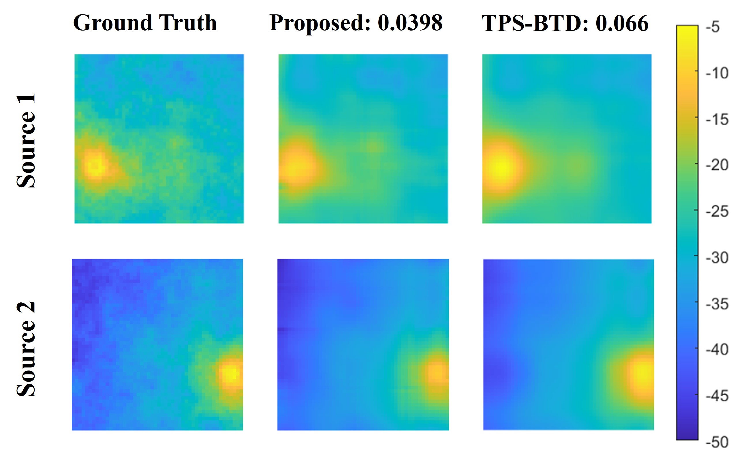
Fig. 2(a) demonstrates that the proposed method achieves more than double the improvement in spectrum reconstruction compared to the TPS-BTD baseline. Furthermore, as demonstrated in Fig. 2(b), it also provides an enhancement in power spectrum map reconstruction exceeding 10%. This highlights its ability to identify multiple sources, even with overlapping spectra, compared to the baseline method. The TPS-BTD method underperforms primarily because selecting an appropriate rank is challenging. Fig. 3 displays a clear visualization of the propagation field under where there is also an accuracy improvement of more than % in reconstructing compared to the baseline method.
V Numerical Results
We adopt model (4) to simulate the power spectrum map in an area for meters, where follows Friis transmission equation, represents the distance from the source. We choose the parameter W, for illustrative purpose. Other values are broadly similar. The number of sources is . The power spectrum is generated by where , is the center of the -th square sinc function, . The sensors are distributed uniformly at random in the area to collect the signal power . The shadowing component in log-scale is modeled using a Gaussian process with zero mean and auto-correlation function , in which correlation distance meters, shadowing variance . The SNR is defines as where the follows Gaussian distribution and is chosen to make the SNR dB. We select the parameter in the kernel function to ensure that it contains at least sensors.
We employ the NMSE of the reconstructed power spectrum map for performance evaluation. Let the NMSE of tensor be , the NMSE of and is of the same form. The performance is compared with the following baselines that are recently developed or adopted in related literature. Baseline 1: Thin plate spline (TPS) [27]. Baseline 2: low-rank tensor completion (LRTC) [28]. Baseline 3: TPS-BTD[21], we first perform TPS, then, the uncertainty is derived and imposed as the restriction on the BTD method.
V-A The Influence of Number of Measurements
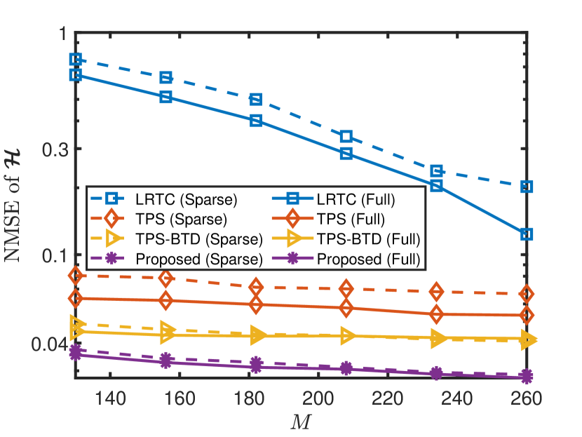
We quantify the power spectrum map reconstruction performance of the proposed method under different number of measurements which is of sampling rate under fixed resolution . We choose the number of frequency bands being for the full observation case and for the sparse observation case, separately. For the sparse observation case, we randomly select the observed frequency bands for the sensors.
Fig. 4 shows the performance of power spectrum reconstruction under both full and sparse observation scenarios. It demonstrates that the proposed method is robust when each sensor only observes random portion of the spectrum. The proposed scheme achieves over a % improvement in reconstruction accuracy in both cases, which translates to roughly % reduction of the measurements to achieve the same NMSE performance. A larger will contribute to a performance gain of the proposed method. The inferior performance of LRTC stems from off-grid sparse observations. Similarly, TPS underperforms because it fails to leverage the correlation property in the frequency domain. TPS-BTD, which relies on TPS interpolation, also falls short as it does not utilize the correlation property effectively.
When the number of measurements increase, the performance of the proposed method under the sparse observation case approaches the full observation case, revealing that exploit a tensor structure can save the number of measurements to attain a similar accuracy.
V-B The Influence of Non-homogeneous Spectrum Observation
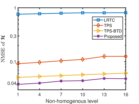
We investigate the influence of the non-homogeneous observation of spectrum on the performance under the sparse spectrum observation. In the homogeneous observation, for each sensor location , we randomly select the frequency bands from the whole bands. As a result, we will have a similar number of sensor measurements for each frequency band. In the non-homogeneous case, we still make that each frequency band have a similar number of sensor measurements. But the difference lies in that for a set of sensor locations, they are with higher probability to collect the first bands, and for another set of sensor locations, they are with higher probability to collect the last bands.
To realize this, we separate the sensors locations to two sets , . Then, we choose the weighted sampling without replacement method to choose bands for each sensor from bands. For the locations in , we choose the weight to be for , and for . For the locations in , we choose the weight to be for , and for . Therefore, the weight serves as a measure of the level of non-homogeneity. For , it is homogeneous with identical weights. As increases, the observations of the spectrum become increasingly non-homogeneous.
Fig. 5 illustrates that the proposed method surpasses the baseline methods and is stable under inhomogeneity of the measurement topology, achieving an improvement of around in reconstruction accuracy. The proposed method effectively handles extremely non-homogeneous spectrum cases and still maintains a significant improvement over the baselines.
V-C The Influence of Different Shadowing Parameters
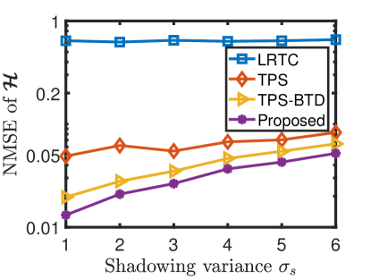
We quantify the reconstruction performance of the proposed method under different shadowing variance and different correlation distance We choose the full observation case , and which corresponding to %.
We first choose correlation distance and varying from to . Fig. 6(a) demonstrates the performance of the proposed method outperforms the baseline methods with an improvement under the shadowing variances . The increasing of the shadowing variance will cause a degradation in the performance of all the methods.
Then, we choose and varying from to . Fig. 6(b) demonstrates that the proposed method surpasses the baseline methods, showing an improvement of across the correlation distances . Additionally, a larger correlation distance contributes to the performance gain.
V-D The Influence of Off-grid Measurements
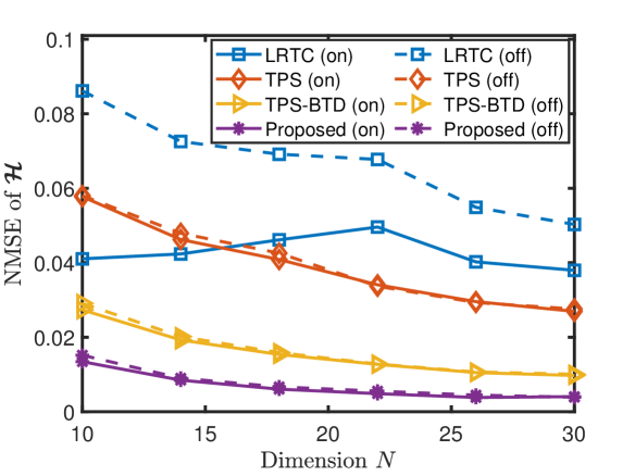
For tensor completion, an off-grid measurements can cause large error and one generally prefers a measurement collecting from the grid center. The proposed method can naturally deal with the off-grid measurements case. Here, we numerically study the influence of off-grid measurements issue through comparing it with on-grid measurements to showcase the proposed method.
The simulation is performed under , , with . Fig. 7 shows that the proposed method outperforms baselines in over improvement in reconstruction accuracy. In addition, the proposed method is stable under off-grid measurements which shows a similar performance between the on-grid and off-grid measurements. This is because the proposed method has an interpolation as a intermediate step, it can deal with the off-grid measurements. The performance between the off-grid and on-grid case approaches at large . The difference between on-grid and off-grid for LRTC is large because the tensor completion method is sensitive to the noise.
VI Conclusion
This paper developed a novel integrated interpolation and BTD approach for reconstructing power spectrum maps. This integrated approach addressed the spatial correlation of power spectrum maps, captured their low-rank characteristics, and reduced errors from off-grid measurements. An algorithm based on alternating least squares and singular value thresholding was developed. Theoretical analysis showed that the incorporation of the BTD structure improved interpolation. Extensive simulations were conducted, demonstrating that the proposed method achieved over % improvement in reconstruction accuracy across various scenarios, such as different numbers of sensors, measurement topology homogeneity, shadowing parameters, and off-grid scenarios.
Appendix A Proof of Theorem 1
Under , the solution for the weighted least-squares problem (14) is
| (26) |
Denote and recall that . From (4), we have,
| (27) |
where .
Applying third order Taylor’s expansion to at the neighborhood of , we have
| (28) |
where is the first order derivative of evaluated at point , is the Hessian matrix of evaluated at point , means , represents third order component, represent the th element in .
Denote and recall . Then, the expression of in (27) can be rearranged into the following matrix form
| (32) |
where is a vector of the residual terms .
Since , the expectation of in (26) can be written as
The variance of can be derived as follows:
| (33) |
Since each sensor measures all the frequency bands, , defined in (12), is identity matrix. Through simple matrix multiplication, the matrix can be derived as follows:
| (34) |
where
with . Here, is a topology matrix that only depends on the sample locations , the grid position , and the kernel function . In addition,
| (35) |
where
with . Likewise, is also a topology matrix that captures the impact from the sample locations.
Thus, Equation (33) is further derived as follows:
| (36) |
Appendix B Proof of Proposition 1
For the error term related to frequency-selective fading , we have
Then, a larger value of will contribute to a smaller value of , vice versa. It can be verified easily that when there is equal-power allocation, i.e., , , attains its largest value , thus attains its smallest value . When there is a power boost in th frequency band, i.e., approaches and others approaches , will attain its smallest value , thus attains its largest value .
For the error term related to measurement noise , we have
It can be verified easily that it attains the largest value when there is equal-power allocation, i.e., , and the smallest value when there is a power boost in th frequency band, i.e., approaches and others approaches . This leads to the result in Proposition 1.
Appendix C Proof of Proposition 2
The derivation follows the same approach for proving Theorem 1, resulting in the local polynomial interpolation error for the th frequency band as
where the result coincides with (22) under . Note that since the frequency-selective fading in (1) and the measurement noise in (2) are assumed to be independent across , given the sensor topology and , the interpolation error is also independent across . Therefore, the averaged interpolation error of all the frequency bands is
Appendix D Proof of Proposition 3
We have the difference value of the variance of interpolation error between the integrated interpolation and BTD approach and conventional frequency-by-frequency interpolation as follows:
| (38) | |||
| (39) |
For (38), the coefficient of can be derived as follows:
For (39), the coefficient of can be derived as follows:
Thus, and the difference is
Appendix E Proof of Proposition 4
The derivation is the same as proving Theorem 1 in Appendix A, except that, due to the sparse observation, (34) becomes
| (40) |
To verify the above result, using Equation (12) and the definition of and , the first element in the matrix is derived as follows:
| (41) |
which equals to , where is defined in (34) and the last equation is because .
Similarly, one can easily show that all the other elements in the matrix equals to the corresponding element in scaled by . Moreover, considering , Equation (35) becomes
| (42) |
Then, the remaining part in Appendix A can be directly applied based on the modified quantities (40) and (42), leading to the following result in Proposition 4.
Appendix F Proof of Theorem 2
Similar to the derivation in (32), the expression of in (43) can be rearranged into the following matrix form
| (44) |
where , is a vector of the residual terms , and
Similar as in Appendix A, the variance of the interpolation error is as follows:
| (45) |
References
- [1] D. Romero and S.-J. Kim, “Radio map estimation: A data-driven approach to spectrum cartography,” IEEE Signal Process. Mag., vol. 39, no. 6, pp. 53–72, 2022.
- [2] D. Gesbert, O. Esrafilian, J. Chen, R. Gangula, and U. Mitra, “Uav-aided rf mapping for sensing and connectivity in wireless networks,” IEEE Wireless Commun., vol. 30, no. 4, pp. 116–122, 2023.
- [3] J. Gao, D. Wu, F. Yin, Q. Kong, L. Xu, and S. Cui, “Metaloc: Learning to learn wireless localization,” IEEE J. Sel. Areas Commun., vol. 41, no. 12, pp. 3831–3847, 2023.
- [4] J. Chen and U. Mitra, “Unimodality-constrained matrix factorization for non-parametric source localization,” IEEE Trans. Signal Process., vol. 67, no. 9, pp. 2371–2386, May 2019.
- [5] X. Mo, Y. Huang, and J. Xu, “Radio-map-based robust positioning optimization for UAV-enabled wireless power transfer,” IEEE Wireless Commun. Lett., vol. 9, no. 2, pp. 179–183, 2019.
- [6] F. Shen, Z. Wang, G. Ding, K. Li, and Q. Wu, “3D compressed spectrum mapping with sampling locations optimization in spectrum-heterogeneous environment,” IEEE Trans. on Wireless Commun., vol. 21, no. 1, pp. 326–338, 2022.
- [7] K. Sato, K. Suto, K. Inage, K. Adachi, and T. Fujii, “Space-frequency-interpolated radio map,” IEEE Trans. Veh. Technol., vol. 70, no. 1, pp. 714–725, 2021.
- [8] K. Sato and T. Fujii, “Kriging-based interference power constraint: Integrated design of the radio environment map and transmission power,” IEEE Trans. Cogn. Commun. Netw., vol. 3, no. 1, pp. 13–25, 2017.
- [9] J. Fan, Local polynomial modelling and its applications: Monographs on statistics and applied probability 66. Routledge, 1996.
- [10] Y. Zhang and S. Wang, “K-nearest neighbors gaussian process regression for urban radio map reconstruction,” IEEE Commun. Lett., vol. 26, no. 12, pp. 3049–3053, 2022.
- [11] M. Hamid and B. Beferull-Lozano, “Non-parametric spectrum cartography using adaptive radial basis functions,” in Proc. IEEE Int. Conf. Acoustics, Speech, and Signal Processing, 2017, pp. 3599–3603.
- [12] S.-J. Kim and G. B. Giannakis, “Cognitive radio spectrum prediction using dictionary learning,” in Proc. IEEE Global Telecomm. Conf., 2013, pp. 3206–3211.
- [13] M. D. Migliore, “A compressed sensing approach for array diagnosis from a small set of near-field measurements,” IEEE Trans. Antennas Propag., vol. 59, no. 6, pp. 2127–2133, 2011.
- [14] H. Sun and J. Chen, “Grid optimization for matrix-based source localization under inhomogeneous sensor topology,” in Proc. IEEE Int. Conf. Acoustics, Speech, and Signal Processing, 2021, pp. 5110–5114.
- [15] D. Schaufele, R. L. G. Cavalcante, and S. Stanczak, “Tensor completion for radio map reconstruction using low rank and smoothness,” in Proc. IEEE Int. Workshop Signal Process. Adv. Wireless Commun., 2019, pp. 1–5.
- [16] Y. Teganya and D. Romero, “Deep completion autoencoders for radio map estimation,” IEEE Trans. Wireless Commun., vol. 21, no. 3, pp. 1710–1724, 2021.
- [17] T. Hu, Y. Huang, J. Chen, Q. Wu, and Z. Gong, “3D radio map reconstruction based on generative adversarial networks under constrained aircraft trajectories,” IEEE Trans. Veh. Technol., vol. 72, no. 6, pp. 8250–8255, 2023.
- [18] G. Zhang, X. Fu, J. Wang, X.-L. Zhao, and M. Hong, “Spectrum cartography via coupled block-term tensor decomposition,” IEEE Trans. Signal Process., vol. 68, pp. 3660–3675, 2020.
- [19] S. Shrestha, X. Fu, and M. Hong, “Deep spectrum cartography: Completing radio map tensors using learned neural models,” IEEE Trans. Signal Process., vol. 70, pp. 1170–1184, 2022.
- [20] H. Sun and J. Chen, “Propagation map reconstruction via interpolation assisted matrix completion,” IEEE Trans. Signal Process., vol. 70, pp. 6154–6169, 2022.
- [21] X. Chen, J. Wang, G. Zhang, and Q. Peng, “Tensor-based parametric spectrum cartography from irregular off-grid samplings,” IEEE Signal Process. Lett., vol. 30, pp. 513–517, 2023.
- [22] H. Sun, J. Chen, and Y. Luo, “Tensor-guided interpolation for off-grid power spectrum map construction,” in Proc. IEEE Int. Conf. Acoust. Speech Signal Process., 2024, to appear.
- [23] H. Sun and J. Chen, “Regression assisted matrix completion for reconstructing a propagation field with application to source localization,” in Proc. IEEE Int. Conf. Acoustics, Speech, and Signal Processing, Singapore, May 2022, pp. 3353–3357.
- [24] A. Graham, Kronecker products and matrix calculus with applications. Courier Dover Publications, 2018.
- [25] L. F. Portugal, J. J. Judice, and L. N. Vicente, “A comparison of block pivoting and interior-point algorithms for linear least squares problems with nonnegative variables,” Mathematics of Computation, vol. 63, no. 208, pp. 625–643, 1994.
- [26] J.-F. Cai, E. J. Candès, and Z. Shen, “A singular value thresholding algorithm for matrix completion,” SIAM Journal on optimization, vol. 20, no. 4, pp. 1956–1982, 2010.
- [27] J. A. Bazerque, G. Mateos, and G. B. Giannakis, “Group-lasso on splines for spectrum cartography,” IEEE Trans. Signal Process., vol. 59, no. 10, pp. 4648–4663, 2011.
- [28] J. Liu, P. Musialski, P. Wonka, and J. Ye, “Tensor completion for estimating missing values in visual data,” IEEE Trans. Pattern Anal. Mach. Intell., vol. 35, no. 1, pp. 208–220, 2013.