Estimation of the electromagnetic field in intermediate-energy heavy-ion collisions

Abstract

We estimate the spacetime profile of the electromagnetic field in head-on heavy-ion collisions at intermediate collision energies $\sqrt{s_{\rm NN}}={\mathcal{O}}(3\;\mathchar 45\relax\;10\;{\rm GeV})$. Using a hadronic cascade model (JAM; Jet AA Microscopic transport model), we numerically demonstrate that the produced field has strength $eE={\mathcal{O}}((30\;\mathchar 45\relax\;60\;{\rm MeV})^{2})$, which is supercritical to the Schwinger limit of QED and is non-negligibly large compared even to the hadron/QCD scale, and survives for a long time $\tau={\mathcal{O}}(10\;{\rm fm}/c)$ due to the baryon stopping. We show that the produced field is nonperturbatively strong in the sense that the nonperturbativity parameters (e.g., the Keldysh parameter) are sufficiently large, which is in contrast to high-energy collisions $\sqrt{s_{\rm NN}}\gtrsim 100\;{\rm GeV}$, where the field is merely perturbative. Our results imply that the electromagnetic field may have phenomenological impacts on hadronic/QCD processes in intermediate-energy heavy-ion collisions and that heavy-ion collisions can be used as a new tool to explore strong-field physics in the nonperturbative regime.

I Introduction

Super dense matter, such as that realized inside a neutron star or even denser, can be produced on Earth by colliding heavy ions at intermediate collision energies $\sqrt{s_{\rm NN}}={\mathcal{O}}(3\;\mathchar 45\relax\;10\;{\rm GeV})$. Such collision experiments have been performed in the Beam Energy Scan program at RHIC [1] and are planned worldwide (e.g., FAIR [2], NICA [3], HIAF [4], J-Parc-HI [5]) to reveal the extreme form of matter in the dense limit and to develop a better understanding of strong interaction, or quantum chromodynamics (QCD). These experimental programs have motivated various theoretical studies, which are mainly aimed at investigating the consequences of the high-density matter and the dynamics of how it can be created during the collisions, e.g., novel phases of QCD at finite density (see Ref. [6] for a review) and the development of various transport models to simulate the realtime collision dynamics such as RQMD [7], UrQMD [8, 9], JAM [10], and SMASH [11].

The purpose of this paper is, rather than pursuing the high-density physics as previously discussed, to point out that a strong electromagnetic field can be created in intermediate-energy heavy-ion collisions. The generation of such a strong electromagnetic field is of interest not only to hadron/QCD physics but also to the area of strong-field physics. For hadron/QCD physics, electromagnetic observables such as di-lepton yields [12, 13, 14, 15], which are promising probes of nontrivial processes induced by the high-density matter, are naturally affected by the presence of a strong electromagnetic field. A correct estimation of the electromagnetic-field profile (and also its implementation into transport-model simulations; cf. Ref. [16, 17]) is, therefore, important when extracting/interpreting signals of the high-density matter from the actual experimental data. As for strong-field physics, the generation of a strong electromagnetic field would provide a unique and novel opportunity to study quantum electrodynamics (QED) in the nonperturbative regime beyond the Schwinger limit $eE_{\rm cr}:=m_{e}^{2}=(0.511\;{\rm MeV})^{2}$ (with $e=|e|$ being the elementary electric charge, $E$ electric field strength, and $m_{e}$ the electron mass). Currently, strong-field physics is driven mainly by high-power lasers (see, e.g., Refs. [18, 19] for reviews). The focused laser intensity of $I=1\times 10^{23}\;{\rm W/cm^{2}}$ (corresponding to $E\approx 10^{-3}\,E_{\rm cr}$) is the current world record [20], which is envisaged to be surpassed by the latest and future facilities such as Extreme Light Infrastructure (ELI) $I={\mathcal{O}}(10^{25}\;{\rm W/cm^{2}})$ [21]. Although the laser intensity is growing rapidly, it is and will remain, for at least the next decade, several orders of magnitude below the Schwinger limit $E_{\rm cr}$. Therefore, it is difficult to study strong-field phenomena with current lasers. This means that a novel method or physical system to realize a strong electromagnetic field is highly demanded.

There exist a number of studies on the generation of a strong electromagnetic field at low- and high-energies both theoretically and experimentally. Let us briefly review them, so as to clarify our motivation to go to the intermediate energy. At low energies, due to the baryon stopping (i.e., the Landau picture [22, 23]), the collided ions stick together at the collision point and form up a gigantic ion with large atomic number $Z={\mathcal{O}}(100)$, and thereby creates a strong Coulomb electric field of the order of $eE\sim(e^{2}/4\pi)Z/R^{2}={\mathcal{O}}((20\;{\rm MeV})^{2})$, where $R={\mathcal{O}}(10\;{\rm fm})$ is the typical radius of the gigantic ion. The produced field is weak compared to the hadron/QCD scale but is far surpassing the Schwinger limit of QED. Thus, it is expected to induce intriguing nonlinear QED processes such as the vacuum decay (see Ref. [24] for a recent analysis), experimental investigation of which has been done around 1980s but is not conclusive yet (see, e.g., Ref. [25] for possible interpretations of the experimental results). On the other hand, at high energies, the Bjorken picture [26] is valid rather than the Landau picture. The colliding ions penetrate with each other without sticking, and hence they do not form up a gigantic ion with large $Z$, unlike the low-energy case. Nevertheless, high-energy heavy-ion collisions are able to produce a very strong electromagnetic field with a different mechanism. Namely, due to a strong Lorentz contraction, the charge density $\rho$ of the incident ions are enhanced by the Lorentz factor $\gamma\approx(\sqrt{s_{\rm NN}}/1\;{\rm GeV})/2$ as $\rho\to\gamma\rho\approx\gamma e\rho_{0}/2$, where $\rho_{0}\approx 0.168\;{\rm fm}^{-3}$ is the nuclear saturation density and we halved it because roughly the half of the ions is composed of charged nucleons (i.e., proton). Due to this enhancement, at central collision events, a strong Coulomb electric field with peak strength $eE\sim e\rho R$, which can exceed the hadron/QCD scale at the RHIC/LHC energy scale $\sqrt{s_{\rm NN}}={\mathcal{O}}(100\;\mathchar 45\relax\;1000\;{\rm GeV})$ and can achieve $eE={\mathcal{O}}(100\;\mathchar 45\relax\;1000\;{\rm MeV})$ [27], is produced at the instant of when the colliding ions maximally overlap with each other [and also a strong magnetic field can be produced in non-central events at the moment when the ions pass through each other due to the Ampère law (see Ref. [28] for a review), which is experimentally utilized to test intriguing nonlinear QED processes such as the photon-photon scattering [29] and the linear Breit-Wheeler process [30, 31]].

Besides the field strength, there is a crucial difference between the low- and high-energy cases: the lifetime of the produced field. The lifetime of the field is long at low energies due to the baryon stopping. For example, it has been shown that the lifetime $\tau$ can reach $\tau={\mathcal{O}}(100\;\mathchar 45\relax\;1000\;{\rm fm}/c)$ for collision energies close to the Coulomb barrier [32, 33, 34]. In contrast, the lifetime is extremely short at high energies. The produced field can survive only for the instance that the colliding ions pass through each other, which is strongly suppressed by the Lorentz factor as $\tau\sim R/\gamma={\mathcal{O}}(0.1\;\mathchar 45\relax\;0.01\;{\rm fm}/c)$ at the RHIC/LHC energy.

The shortness of the lifetime $\tau$ significantly affects the nonperturbativity of the physics induced by the strong field. Namely, no matter how strong a field is, the physics has to be perturbative if it is short-lived. The low-order perturbation theory becomes sufficient in such a limit, and therefore the physics becomes “trivial” in the sense that it is not very different from the usual electromagnetic processes in the vacuum. Intuitively, this is simply because there is no time for the finite field to have multiple interactions with a particle. To be more quantitative, suppose we have, as an example, an electric field with peak strength $E_{0}$ and lifetime $\tau$, and consider the vacuum pair production by such a strong electric field, ${\rm vacuum}+E\to e^{+}+e^{-}$. For this case, the interplay between the nonperturbative and perturbative pair production is controlled by two dimensionless quantities [35, 36, 37, 38, 39, 40, 41, 42, 43, 44],

$$\xi(m):=\frac{eE_{0}\tau}{m}\ \ {\rm and}\ \ \nu:=eE_{0}\tau^{2}\;.$$ (1)

Note that the parameter $\xi$ is known as the Keldysh parameter [45] and, depending on the context, is also called the classical nonlinearity parameter [19]. The mass $m$ is the mass of the particle to be produced. For enough strong and long-lived fields such that $\xi,\nu\gg 1$, the pair production becomes nonperturbative in the sense that the rate of the pair production acquires a non-analytic dependence in $e$ and $E_{0}$ as $\propto\exp[-({\rm const.})\times(m^{2}/eE_{0})]$. In the opposite limit, $\xi,\nu\ll 1$, it becomes purely perturbative, i.e., the low-order perturbative treatment becomes sufficient, meaning that the rate only has the power dependence in $e$ and $E_{0}$ as $\propto(eE_{0}/m^{2})^{n}$ ($n\in{\mathbb{N}}$). This example of the vacuum pair production clearly demonstrates that the supercriticality $eE_{0}\gtrsim m^{2}$ is not sufficient to guarantee the nonperturbativity of strong-field processes. One must, thus, pay attention to the magnitude of the lifetime $\tau$, or the resulting $\xi$ and $\nu$, as well, in addition to the strength $E_{0}$. In terms of these nonperturbativity parameters (1), high-energy heavy-ion collisions at the typical RHI/LHC scale correspond to $\nu={\mathcal{O}}(0.1)$ and $\xi={\mathcal{O}}(100)$ for electron $m=m_{e}$ and ${\mathcal{O}}(1)$ for pion $m=m_{\pi}\approx 140\;{\rm MeV}$. This means, although $\xi$ can be nonperturbatively large for the QED scale $m=m_{e}$ due to the largeness of the field strength, $\nu$ always remains perturbatively small due to the shortness of the lifetime. For the hadron/QCD scale $m=m_{\pi}$, neither $\xi$ nor $\nu$ can be nonperturbative. Therefore, in either case of QED or QCD, the pair production cannot be nonperturbative, implying that strong-field physics in the nonperturbative regime cannot be explored with the field produced in high-energy heavy-ion collisions. This naive argument, based on the “order parameters” of the vacuum pair production, is consistent with the actual experimental results. There have been observations of next-leading-order QED processes such as light-by-light scattering [29] and linear Breit-Wheeler pair production [30], in which the experimental results are consistent with perturbative QED calculations and no signatures of higher-order nonlinear effects have been detected.

We are now in a position to address the advantage of going to intermediate energies. It is natural to expect that the electromagnetic field generated in intermediate-energy heavy-ion collisions should have characteristics between the low- and high-energy cases. Namely, although the field strength would be weaker than that in the high-energy case, it should be stronger than that in the low-energy case. This means that the produced field will remain much stronger than the Schwinger limit of QED and may still be comparable to the hadron/QCD scale. As for lifetime, we can naturally expect that the field produced at intermediate energies should survive longer than the high-energy field. If this is true, it overcomes the problem of the short lifetime in the high energy limit, while maintaining a sufficiently large field strength. Hence, it enables us to access the strong-field physics in the nonperturbative regime. It is therefore worthwhile to investigate the generation of a strong electromagnetic field in intermediate-energy heavy-ion collisions and to make a realistic estimate to clarify whether this is the case, and, if so, how important it is.

Based on the motivations explained thus far, we would like to make a realistic estimate of the electromagnetic field in intermediate-energy heavy-ion collisions based on a hadron-transport-model simulation. Indeed, neither the Landau nor the Bjorken picture is complete at intermediate energies (cf. Ref. [46] as a related for vorticity estimation). Accordingly, the generation mechanism of the electromagnetic field is more involved compared to the low- and high-energy limits, and hence it is impossible to carry out a simple analytic estimate at intermediate energies. In particular, dynamical effects become more important than the other energy regimes. For example, both elastic- and inelastic- multiple collision processes among the constituent nucleons are important to determine the sticking or non-sticking of the colliding ions. Hadrons are produced or decay during the time evolution through the inelastic processes, meaning that the simple but widely-used modeling based the Liénard-Wiechert potential of the electromagnetism is not applicable. The Lorentz contraction comes into play, unlike at the low energy limit, but is not as strong as that at the high energy, and therefore hadrons consisting of the colliding ions need to be treated as anisotropic objects with finite size. All of those dynamical effects can be taken into account systematically by using established hadron-transport models of heavy-ion collisions. In this work, we adopt JAM (Jet AA Microscopic transport model) [10, 47]. JAM is a hadronic cascade model to simulate the realtime dynamics of heavy-ion collisions. In addition to elastic hadron-hadron scatterings, inelastic processes are implemented in JAM via resonance production, soft-string excitation, and multiple mini-jet production, so that it can be applied to a wide range of collision energies from $\sqrt{s_{\rm NN}}={\mathcal{O}}(2\;{\rm GeV})$ up to ${\mathcal{O}}(100\;{\rm GeV})$. More details of JAM, including its comparison with other models, can be found in, e.g., Ref. [48].

This paper is organized as follows. We first explain our numerical setup and how we calculate the electromagnetic field with JAM in Sec. II. We then present the numerical results in Sec. III that include the spacetime profiles of the charge density (Sec. III.1) and the resulting electromagnetic field (Sec. III.2), the time evolution of the peak strength (Sec. III.3), and the corresponding nonperturbativity parameters $\xi$ and $\nu$ to demonstrate that the field is nonperturbatively strong (Sec. III.4).

Notation: Our metric is the mostly minus, i.e., $g^{\mu\nu}:={\rm diag}(+1,-1,-1,-1)$. Spatial three vectors are indicated by the bold letters, e.g., $x^{\mu}:=(t,{\bm{x}})$ for spacetime coordinates and $A^{\mu}=(A^{0},{\bm{A}})$ for the four-vector potential. We take the $z$-axis along the beam direction and write ${\bm{x}}=:(x,y,z)=:({\bm{x}}_{\perp},z)$.

II Numerical recipe

II.1 Calculation program

We wish to calculate the electric ${\bm{E}}$ and magnetic ${\bm{B}}$ fields in heavy-ion collisions at intermediate collision energies. The electromagnetic fields are given by

$${\bm{E}}:=-\partial_{t}{\bm{A}}-{\bm{\nabla}}A^{0}\ \ {\rm and}\ \ {\bm{B}}:={\bm{\nabla}}\times{\bm{A}}\;,$$ (2)

where $A^{\mu}$ is the retarded vector potential,

$$A^{\mu}(t,{\bm{x}}):=\frac{1}{4\pi}\int{\rm d}^{3}{\bm{x}}^{\prime}\frac{J^{\mu}(t-|{\bm{x}}-{\bm{x}}^{\prime}|,{\bm{x}}^{\prime})}{|{\bm{x}}-{\bm{x}}^{\prime}|}\;,$$ (3)

with $J^{\mu}$ being the total electric current carried by the charged particles in the collisions. In the present paper, we focus on the event-averaged values of $O={\bm{E}},{\bm{B}}$ and take the event averaging of Eq. (2) as

$$O:=\frac{1}{N}\sum_{i=1}^{N}O_{i}\;,$$ (4)

where $O_{i}$ is the event-by-event result and $N$ is the total number of the events. Note that event-by-event fluctuations may be important in actual experiments (see also Ref. [27] for the high-energy case). For example, it has been argued in Refs. [49, 50, 51] that the maximum value of the baryon density can fluctuate event-by-event by more than 30 % at intermediate energies. Such large fluctuations of the baryon density $\rho_{\rm B}$ imply that the charge density $\rho/e\approx\rho_{\rm B}/2$ should also fluctuate, and so does the resulting electromagnetic field. We shall report the event-by-event fluctuations of the electromagnetic fields in intermediate-energy heavy-ion collisions in a forthcoming paper.

We evaluate the electromagnetic field (2) numerically as follow. We first calculate the electric current $J^{\mu}$ with JAM. JAM calculates the phase-space distributions of hadrons in heavy-ion collisions $({\bm{x}}_{n}(t),p^{\mu}_{n}(t))$, where the subscript $n$ labels the hadrons in a collision event. The electric current $J^{\mu}$ at a position $(t^{\prime},{\bm{x}}^{\prime})$ is then given in terms of the JAM phase-space distribution as

$$J^{\mu}(t^{\prime},{\bm{x}}^{\prime}):=\sum_{n\in{\rm all\;hadrons}}\frac{p^{\mu}_{n}(t^{\prime})}{p^{0}_{n}(t^{\prime})}\rho_{n}(t^{\prime},{\bm{x}}^{\prime})\;,$$ (5)

where $\rho_{n}$ is the charge density of a single charged hadron. In JAM, hadrons are treated as if they are point-like, and hence the charge density of each hadron is localized strictly at ${\bm{x}}_{n}$. Hadrons are finite-sized in reality, motivated by which we smear the charge density by using the (relativistic) Gaussian distribution:

$$\rho_{n}(t^{\prime},{\bm{x}}^{\prime}):=q_{n}\frac{\gamma_{n}(t^{\prime})}{(\sqrt{2\pi}\sigma)^{3}}$$

$$\times\exp\left[-\frac{|{\bm{x}}^{\prime}-{\bm{x}}_{n}(t^{\prime})|^{2}+\gamma_{n}^{2}(t^{\prime})\left({\bm{v}}_{n}(t^{\prime})\cdot({\bm{x}}^{\prime}-{\bm{x}}_{n}(t^{\prime}))\right)^{2}}{2\sigma^{2}}\right]\;,$$

where $q_{n}$ is the electric charge, $\sigma$ the smearing width, and $\gamma:=\sqrt{1-{\bm{v}}_{n}^{2}}:=\sqrt{1-({\bm{p}}_{n}/p^{0}_{n})^{2}}$ the Lorentz factor for the $n$-th hadron.

Once the electric current $J^{\mu}$ is obtained with JAM, can we calculate the retarded vector potential $A^{\mu}(t,{\bm{x}})$ by carrying out the ${\bm{x}}^{\prime}$ integration according to Eq. (3) at each spacetime point $(t,{\bm{x}})$. This can be done with the standard numerical integration schemes, e.g., the Gauss-Legendre quadrature method, which we have adopted in this work.

In the default setting of JAM, the simulation starts from some initial time $t_{\rm in}=:0$, around which the incident ions start to collide. The JAM hadron phase-space data is, thus, available only later than $t_{\rm in}$, so is the electric current $J^{\mu}$ (5). To perform the integration (3), the information of the electric current at time $t^{\prime}=t-|{\bm{x}}-{\bm{x}}^{\prime}|$, which can be earlier than $t_{\rm in}$ (when $|{\bm{x}}-{\bm{x}}^{\prime}|>t-t_{\rm in}$), is needed. To get the electric current before the initial time $t_{\rm in}$, we extrapolate the phase-space data at the initial time $t=t_{\rm in}$ by assuming that the hadrons that constitutes the incident ions go straight trajectories in the phase-space without any interactions:

$$\begin{split}&{\bm{x}}_{n}(t<t_{\rm in}):={\bm{x}}_{n}(t_{\rm in})+(t-t_{\rm in})\frac{{\bm{p}}_{n}(t_{\rm in})}{p^{0}_{n}(t_{\rm in})}\;,\\ &p^{\mu}_{n}(t<t_{\rm in}):=p^{\mu}_{n}(t_{\rm in})\;.\end{split}$$ (6)

Having calculated the retarded vector potential $A^{\mu}$ (3), can we obtain the electromagnetic fields via the differentiation (2). We in this work have adopted the standard central difference method with discretizing the ${\bm{x}}$ coordinates with uniform meshes.

II.2 Numerical parameters

Ion species		${}^{197}{\rm Au}$
Collision energy $\sqrt{s_{\rm NN}}$		2.4, 3.0, 3.5, 3.9, 4.5, 5.2, 6.2, 7.2, 7.7, 9.2, and 11.5 GeV
Impact parameter $b$		0 fm
Gaussian smearing width $\sigma$		1 fm
Total event number $N$		100
Discretization of time $t$		$t\in[0,30]\;{\rm fm}/c$ with $\Delta t=0.5\;{\rm fm}/c$
Discretization of ${\bm{x}}=(x,y,z)$		$x,y,z\in[-30,+30]\;{\rm fm}$ with $(n_{x},n_{y},n_{z})=(121,121,121)$ sites
		(a uniform 3D lattice with $\Delta x=\Delta y=\Delta z=0.5\;{\rm fm}$)
Discretization of ${\bm{x}}^{\prime}=(x^{\prime},y^{\prime},z^{\prime})$		$x^{\prime},y^{\prime},z^{\prime}\in[-30,+30]\;{\rm fm}$ with $(n_{x^{\prime}},n_{y^{\prime}},n_{z^{\prime}})=(120,120,120)$ sites
		(a non-uniform 3D lattice for the Gauss-Legendre quadrature method)

Table 1: Parameters adopted in the numerical simulation.

We summarize the numerical parameters adopted in the present work in Table 1.

Using JAM, we simulate head-on (i.e., the impact parameter $b$ is strictly fixed at $b=0$) collisions of gold ions at the intermediate energies $\sqrt{s_{\rm NN}}=2.4,3.0,3.5,3.9,4.5,5.2,6.2,7.2,7.7,9.2$, and $11.5$. Several advanced options are available in JAM (such as the mean-field potential and hybrid hydrodynamic simulation), which we switch off and run JAM with the default setting to carry out the most basic hadronic cascade simulation. Note that, although we have concentrated on gold collisions as a first step to study the electromagnetic-field physics in intermediate-energy heavy-ion collisions, it is an interesting question to consider other ion species. In particular, deformed ions such as uranium and also asymmetric collisions such as Au + Cu (see, e.g., Refs. [52, 53, 54] at high energies) would be of interest, in which case the resulting electromagnetic fields should have a preferred direction due to the collision geometry, leading to observable effects such as a charged $v_{1}$ flow. The impact parameter dependence is also an interesting issue. With finite impact parameters magnetic field shall dominate, while electric field does so in head-on events as we shall demonstrate below. We shall report the interplay of the dominance between the electric and magnetic fields in a future publication.

We have five numerical parameters in the evaluation of the electromagnetic field outlined in Sec. II.1: the event number $N$, the smearing width $\sigma$, and the discretizations of $t,{\bm{x}}$, and ${\bm{x}}^{\prime}$. To reduce the numerical cost, we are reluctant to take a relatively small event number $N=100$, although the residual event-by-event fluctuations do not look very significant after the event averaging as we show later. We shall use the particular value of the smearing width $\sigma=1\;{\rm fm}$ for all hadron species, which is physically motivated by that the typical size of a nucleon is of the order of $1\;{\rm fm}$ and is a common choice in the literature. We have checked that the numerical results are less sensitive to the value of $\sigma$ after taking the event averaging. We have also carefully checked that the lattice volumes of ${\bm{x}}$ and ${\bm{x}}^{\prime}$ and the mesh sizes $\Delta t,\Delta{\bm{x}}$, and $\Delta{\bm{x}}^{\prime}$ are sufficiently large and fine, respectively, in such a way that the numerical results are not sensitive to them. Note that, for the present parameters, a single numerical simulation (per energy) consumes ${\mathcal{O}}(20\;{\rm GB})$ RAM and takes about a few days with a standard GPU computer available on the market.

III Numerical results

We present the numerical results obtained with the recipe outlined in Sec. II. The main result is that an electric field which is non-perturbatively strong and long-lived can be created in intermediate-energy heavy-ion collisions; see Sec. III.4, in particular Fig. 4. Before getting there, we discuss the generation of such a strong electric field step by step. We first demonstrate in Sec. III.1 that a highly-charged matter $\rho/e={\mathcal{O}}(0.5\;{\rm fm}^{-3})$, as a reminiscent of the dense baryon matter, is realized at intermediate energies. The highly-charged matter sources a strong electric field, whose spacetime profile shall be discussed in Sec. III.2. We shall discuss the intensity and the lifetime of the produced electric field in detail in Sec. III.3 and show in Sec. III.4 that it can be nonperturbatively strong and long-lived, in contrast to what is realized at high energies.

III.1 Spacetime profile of the charge density

Fig. LABEL:fig:1 shows the spacetime profile of the charge density. The key observation is that intermediate-energy heavy-ion collisions can realize a high charge density, typically of the order of $\rho/e={\mathcal{O}}(0.5\;{\rm fm}^{-3})$, for a relatively long time $\tau={\mathcal{O}}(10\;{\rm fm}/c)$. The magnitude of the charge density is roughly ${\mathcal{O}}(5)$ times greater than that of an usual charged ion at rest $\rho/e\approx\rho_{0}/2\approx 0.08\;{\rm fm}^{-3}$. This highly-charged matter sources a strong electric field, as we shall demonstrate later.

There are two important physics that contribute to the creation of the highly-charged matter. The first one is the Lorentz contraction. Due to the Lorentz contraction in the beam direction, the incident ions are not spherical, but anisotropic, and the longitudinal size is shortened as $R\to R/\gamma\approx(13\;{\rm fm})/(\sqrt{s_{\rm NN}}/1\;{\rm GeV})$, where $R\approx(1.1\;{\rm fm})\times A^{1/3}\approx 6.4\;{\rm fm}$ is the radius of a gold ion $A=197$ at rest and we used $2\gamma\approx(\sqrt{s_{\rm NN}}/1\;{\rm GeV})$. Accordingly, the charge density is enhanced from that at rest by the Lorentz factor $\gamma$ and hence becomes larger with collision energy as $\rho/e\approx\gamma\times\rho_{0}/2\approx(0.04\;{\rm fm}^{-3})\times(\sqrt{s_{\rm NN}}/1\;{\rm GeV})$. The collision dynamics can roughly be understood as an overlapping process of these two Lorentz-contracted ions. The maximum charge density is then achieved when the two ions maximally overlap with each other. As a zero-th order approximation, we may neglect the interaction between the ions and hence assume that they just pass through each other during a collision. Then, the maximum can be estimated as $\max\rho/e\approx 2\times\rho/e\approx(0.08\;{\rm fm}^{-3})\times(\sqrt{s_{\rm NN}}/1\;{\rm GeV})$ and the time of which achieved as $t_{\rm max}\approx 2R/\gamma\approx(26\;{\rm fm}/c)/(\sqrt{s_{\rm NN}}/1\;{\rm GeV})$. These estimates are in rough agreement with the numbers shown Fig. LABEL:fig:1.

The second is the interaction (i.e., the baryon stopping), which is especially important in determining the lifetime of the highly-charged matter. The importance of the interaction is evident in Fig. LABEL:fig:1. If it is non-interacting, the charge density should exhibit a two-peak structure after the maximum, i.e., the collided ions pass through each other and leave nothing in the mid-rapidity $z\approx 0$ (the Bjorken picture [26]). This is not the case in Fig. LABEL:fig:1, which shows that the density is single-peaked at the mid-rapidity after the collision. In other words, the interaction makes it difficult for the colliding ions to penetrate each other, instead causing them to merge at the point of collision (the Landau picture [22, 23]). The interaction makes the lifetime $\tau$ of the highly-charged matter longer, compared to what is naively expected from the Bjorken picture $\tau\approx 2R/\gamma\approx(26\;{\rm fm}/c)/(\sqrt{s_{\rm NN}}/1\;{\rm GeV})$. For example, at $\sqrt{s_{\rm NN}}=3.0\;{\rm GeV}$, a relatively dense charge state $\rho/e\gtrsim 0.1\;{\rm fm}^{-3}$ appears around $t\approx 2\;{\rm fm}/c$ and survives until $t\approx 18\;{\rm fm}/c$, whose lifetime $\tau\approx 18-2\;{\rm fm}/c=16\;{\rm fm}/c$ is much longer than the naive Bjorken estimate $\tau\approx 26/3\;{\rm fm}/c\approx 9\;{\rm fm}/c$. The interaction effect is non-negligible and hence a highly-charged matter with a relatively long lifetime is realized in the intermediate energy values $\sqrt{s_{\rm NN}}={\mathcal{O}}(3\;\mathchar 45\relax\;10\;{\rm GeV})$.

III.2 Spacetime profile of the produced field

The highly-charged matter created in intermediate-energy heavy-ion collisions (see Fig. LABEL:fig:1) produces a strong electric field. To show this, we plot, in Fig. LABEL:fig:2, an electromagnetic Lorentz invariant,

$${\mathcal{F}}:={\bm{E}}^{2}-{\bm{B}}^{2}\;.$$ (7)

Note that the other invariant ${\mathcal{G}}:={\bm{E}}\cdot{\bm{B}}$ is found to be vanishing (up to residual event-by-event fluctuations). This is reasonable, since we have no electric current ${\bm{J}}$ to produce a macroscopic magnetic field in central collision events and hence ${\bm{B}}\approx{\bm{0}}$. This also means

$${\mathcal{F}}\approx{\bm{E}}^{2}\;.$$ (8)

That is, the produced field is electric, which is also evident in Fig. LABEL:fig:2 that the sign of ${\mathcal{F}}$ is always positive. It is thus convenient to introduce an effective electric field strength $E_{\rm eff}$ such that

$$E_{\rm eff}:=\sqrt{{\mathcal{F}}}\;.$$ (9)

Fig. LABEL:fig:2 shows that the typical strength of the produced electric field is $e^{2}{\mathcal{F}}={\mathcal{O}}(10^{6\;\mathchar 45\relax\;7}\;{\rm MeV}^{4})$, corresponding to $eE_{\rm eff}={\mathcal{O}}((30\;\mathchar 45\relax\;60\;{\rm MeV})^{2})$. The created field is strong in the sense that it is far beyond the Schwinger limit of QED, $eE_{\rm cr}=m_{e}^{2}=(0.511\;{\rm MeV})^{2}$. It is not supercritical to the hadron/QCD scale, $m_{\pi}\approx 140\;{\rm MeV}$, but still is non-negligibly strong $eE_{\rm eff}={\mathcal{O}}((30\;\%\times m_{\pi})^{2})$, implying that it can affect hadron/QCD processes. The produced field also has a sufficiently large spacetime volume $\tau\times V={\mathcal{O}}(10\;{\rm fm}/c)\times{\mathcal{O}}((10\;{\rm fm})^{3})$ because of the baryon stopping and of that the highly-charged matter has a macroscopically large spatial volume $\propto R^{3}/\gamma$.

Let us have a closer look at the spacetime structure of the produced field. First, the produced field has a donuts-like spatial structure, with peaks located around where the charge density vanishes (see Fig. LABEL:fig:1). Namely, the effective field strength $E_{\rm eff}$ is zero at the collision point ${\bm{x}}\approx{\bm{0}}$, and, as going away from the collision point, $E_{\rm eff}$ increases almost linearly $\propto|{\bm{x}}|$ and then decreases quadratically $\propto 1/|{\bm{x}}|^{2}$ after it gets peaked. These are the direct consequences of the Gauss law ${\rm div}\,{\bm{E}}=\rho$ (and is similar to the textbook exercise of the electric field produced by a uniformly charged sphere; see, e.g., Jackson [55]).

Second, the field strength in the transverse plane (the bottom panel in Fig. LABEL:fig:2) increases with collision energy $\sqrt{s_{\rm NN}}$, while that along the beam direction (the top panel in Fig. LABEL:fig:2) is less sensitive to $\sqrt{s_{\rm NN}}$ and is weaker than that in the transverse plane. This is a reminiscent of the anisotropic structure of the charged matter due to the Lorentz contraction (see Fig. LABEL:fig:1) and can be understood simply with the Gauss law. For simplicity, let us model the matter as a uniformly charged short cylinder, with radius $|{\bm{x}}_{\perp}|\leq R$ and length $|z|\leq R/\gamma$. Then, the Gauss law tells us that the field strength is maximized along the longitudinal direction at the ends of the charged cylinder $|z|=R/\gamma$ and the corresponding strength is $E=\rho R/\gamma$. Similarly, the maximum in the transverse plane is $E=\rho R/2$ at $|{\bm{x}}_{\perp}|=R$. Thus, the field strength in the transverse plane is enhanced by the anisotropy factor $\gamma$ compared to that along the longitudinal axis.

Note that the charge density $\rho$ can roughly be estimated as a simple overlapping of two Lorentz-contracted ions $\rho/e\approx\gamma\rho_{0}$ (see Sec. III.1). Therefore, the maximum field strength over the space can be estimated, by using the simple modeling in the last paragraph, as $eE\approx e^{2}\gamma\rho_{0}R/2\approx((\sqrt{s_{\rm NN}}/1\;{\rm GeV})^{1/2}\times 31\;{\rm MeV})^{2}$. This simple estimate is in rough agreement with the actual numbers shown in Fig. LABEL:fig:2 (albeit a bit overestimating, which we discuss in Sec. III.3).

Third, the produced field expands faster with increasing collision energy. For lower energies $\sqrt{s_{\rm NN}}\lesssim 5\;{\rm GeV}$, the expansion is negligible and the field is roughly staying around the original position created. In contrast, for higher energies $\sqrt{s_{\rm NN}}\gtrsim 5\;{\rm GeV}$, the expansion becomes significant and the field moves almost at the speed of light. For the longitudinal expansion, this is a natural consequence that the Bjorken picture begins to be effective for higher energies. Although the Landau picture dominates in the intermediate-energy regime as we have explained in Sec. III.1, it is also true that the Bjorken picture is becoming effective for higher energies, which can be observed in Fig. LABEL:fig:1 from that the charged matter expands in the beam direction after created and begins to exhibit a two-peak structure at, e.g., $\sqrt{s_{\rm NN}}=7.2\;{\rm GeV}$. The expansion also becomes faster in the transverse direction, simply because the typical kinetic energy of the particles in the collision system increases with collision energy, allowing them to move faster.

III.3 Field strength

Having observed the generation of a strong electric field in intermediate-energy heavy-ion collisions, we turn to discuss more quantitative aspects of the produced field, in particular the peak field strength over the space.

We first discuss the time evolution of the field strength; see Fig. LABEL:fig:3 (i). The strength gets maximized when the incident ions overlap with each other the most and shows up a sharp peak at around $t\approx(26\;{\rm fm}/c)/(\sqrt{s_{\rm NN}}/1\;{\rm GeV})$ (within the non-interacting estimate; see Sec. III.1). After the peak, the field strength decays rather slowly, as the collision remnant can survive in the mid-rapidity region due to the baryon stopping, and consequently the field can maintain its strength for a relatively long time. For example, a single ion at rest has a field strength of $eE\lesssim e^{2}(\rho_{0}/2)R/3\approx 25\;{\rm MeV}$, above which strength is kept for more than ${\mathcal{O}}(15\;{\rm fm}/c)$ in intermediate-energy heavy-ion collisions.

The peak in Fig. LABEL:fig:3 (i) becomes larger and sharper with increasing collision energy. This is also evident in Fig. LABEL:fig:3 (ii) and (iii), which show, respectively, the maximum strength of the peak, $\max E_{\rm eff}$, and the full width at the half maximum of $E_{\rm eff}$ (FWHM),

$$\tau:=\int_{E_{\rm eff}(t)>\max E_{\rm eff}/2}{\rm d}t\;.$$ (10)

Note that the FWHM (10) can naturally be regarded as the lifetime of the field produced, and so we use Eq. (10) to define the lifetime in what follows.

The maximum peak field strength increases with collision energy [see Fig. LABEL:fig:3 (ii)], as anticipated with the simple estimate $eE\approx e^{2}\gamma\rho_{0}R/2\approx((\sqrt{s_{\rm NN}}/1\;{\rm GeV})^{1/2}\times 31\;{\rm MeV})^{2}$ that we made in Sec. III.2. The key point is the enhancement of the charge density by the Lorentz contraction, which yields to the energy dependence. Although the simple estimate can capture the qualitative feature of the peak field strength, it fails at the quantitative level mainly because the modeling with a uniformly-charged short cylinder is crude. In particular, the actual charge distribution (see Fig. LABEL:fig:1) is tailed and thus the charge extends more than the rigid cylinder distribution, which makes the actual peak field strength smaller than the simple estimate. Indeed, we find

$$\max\sqrt{eE_{\rm eff}}=\left(\frac{\sqrt{s_{\rm NN}}}{1\;{\rm GeV}}\right)^{1/2}\times 22.38\;{\rm MeV}\;,$$ (11)

which has the smaller coefficient ($31\;{\rm MeV}\to 22\;{\rm MeV}$), can fit the numerical result well.

The lifetime (10) decreases with collision energy [see Fig. LABEL:fig:3 (ii)], which is essentially due to the Lorentz contraction. The typical lifetime of the field is determined by that of the highly-charged matter. Therefore, $\tau\approx 2R/\gamma\approx(26\;{\rm fm}/c)/(\sqrt{s_{\rm NN}}/1\;{\rm GeV})$ in the non-interacting limit (see Sec. III.1). In reality, however, the interaction is important, especially for lower energies $\sqrt{s_{\rm NN}}\lesssim 5\;{\rm GeV}$, and thus the naive non-interacting estimate only gives a poor fit at the quantitative level. The interaction makes the lifetime considerably longer. We numerically find that such an interaction effect can be reproduced well with a higher-order term $\propto s_{\rm NN}^{-1}$, added to the naive $s_{\rm NN}^{-1/2}$ dependence, and the best fitting curve is found to be

$$\tau =\left(\frac{\sqrt{s_{\rm NN}}}{1\;{\rm GeV}}\right)^{-1}\times 14.89\;{\rm fm}/c$$

$$\quad+\left(\frac{\sqrt{s_{\rm NN}}}{1\;{\rm GeV}}\right)^{-2}\times 83.45\;{\rm fm}/c\;.$$ (12)

Note that the fitting curve (12) does not reproduce the coefficient of the naive estimate, $26\;{\rm fm}/c$, even in the limit of $\sqrt{s_{\rm NN}}\to\infty$. This can be understood as an indication that the Bjorken picture cannot be complete and the interaction is important at intermediate energies.

We emphasize that the lifetime is affected significantly by the interaction and made considerably longer, while the peak strength is less affected. Accordingly, the lifetime is more dependent on collision energy than the peak strength is. As we see shortly below, this shall be the essence why we can have a nonperturbatively strong electric field in intermediate-energy heavy-ion collisions, in particular for $\sqrt{s_{\rm NN}}\lesssim 5\;{\rm fm}/c$, where the interaction becomes more important.

III.4 Nonperturbativity

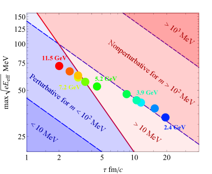
Figure 4: Sensitivity plot for nonperturbativity of the produced electric field in intermediate-energy heavy-ion collisions. The dots represent the characteristics of the field $(\tau,\max\sqrt{eE_{\rm eff}})$ extracted from Fig. LABEL:fig:3 at each collision energy $\sqrt{s_{\rm NN}}$, ranging from $\sqrt{s_{\rm NN}}=2.4\;{\rm GeV}$ (blue), 3.0, 3.5, 3.9, 4.5, 5.2, 6.2, 7.2, 7.7, 9.2, to $11.5\;{\rm GeV}$ (red). The lines represent the nonperturbativity parameters (1): $1=\xi(10\;{\rm MeV})$ (bottom blue dashed), $1=\xi(10^{2}\;{\rm MeV})$ (middle blue dashed), $1=\xi(10^{3}\;{\rm MeV})$ (top blue dashed), and $1=\nu$ (red). Those lines set “phase boundaries” of the nonperturbativity (of the vacuum pair production). The red regions $\xi(m),\nu>1$ are nonperturbative (for mass scales $m$), while it is perturbative in the blue regions $\xi(m),\nu<1$.

As one of the possible “order parameters” for the nonperturbativity of a strong field, we calculate the nonperturbativity parameters $\xi$ and $\nu$ (1) and discuss the sensitivity region in intermediate-energy heavy-ion collisions. The result is shown in Fig. 4. It clearly shows that intermediate-energy heavy-ion collisions, in particular with $\sqrt{s_{\rm NN}}\lesssim 5\;{\rm fm}/c$, can access the nonperturbative regime. Namely, although higher collision energies $\sqrt{s_{\rm NN}}\gtrsim 5\;{\rm fm}/c$ are advantageous in that the field strength is strong, which can be comparable even to the hadron/QCD scale, it is disadvantageous in that the lifetime gets extremely short and accordingly the physics has to be purely perturbative. On the other hand, although the achievable field strength is weaker in lower collision energies $\sqrt{s_{\rm NN}}\lesssim 5\;{\rm fm}/c$, it is still much stronger than the critical strength of QED and is non-negligible to the hadron/QCD scale, and also the lifetime can be very long, allowing us to enter the nonperturbative regime.

Using the fitting results, Eq. (11) for $\max\sqrt{eE_{\rm eff}}$ and Eq. (12) for $\tau$, we find that the nonperturbativity parameters $\xi$ and $\nu$ can be parametrized as

$$\xi =\frac{37.27\;{\rm MeV}+\left(\frac{\sqrt{s_{\rm NN}}}{1\;{\rm GeV}}\right)^{-1}\times 208.93\;{\rm MeV}}{m}\;,$$ (13)

$$\nu =\left(9.34\times s_{\rm NN}^{-3/4}+1.67\times s_{\rm NN}^{-1/4}\right)^{2}\approx 87.18\times s_{\rm NN}^{-3/2}\;.$$

It is clear that both $\xi$ and $\nu$ increase with decreasing collision energy $\sqrt{s_{\rm NN}}$, i.e., lowering the energy is more beneficial for the nonperturbativity. The interaction effect in the Landau stopping regime gives a significant contribution here, as the dominant $s_{\rm NN}^{-1/2}$ and $s_{\rm NN}^{-3/2}$ dependencies in $\xi$ and $\nu$, respectively, arise from the $s_{\rm NN}^{-1}$ term in the lifetime $\tau$ (12), which we have added to account for the interaction effect.

For clarity, we remark that the meaning of the “nonperturbative” in Fig. 4 is just that the physical observable (or, to be precise, the number of particle and anti-particle pairs with mass $m$ produced from the vacuum by a strong electric field $E$ [35, 36, 37, 38, 39, 40, 41, 42, 43, 44]) acquires a nonperturbative dependence $\propto\exp[-({\rm const})\times m^{2}/eE]$. In other words, being in the nonperturbative regime does not necessarily guarantee the significance of the nonperturbative effect and/or its detectability in actual experiments. In fact, unless we have a field strength comparable to or exceeding the mass scale $eE\gtrsim m^{2}$, the effect is strongly suppressed by the exponential $\propto\exp[-({\rm const})\times m^{2}/eE]$ and is simply negligible. For example, the lowest energy $\sqrt{s_{\rm NN}}=2.4\;{\rm GeV}$ is nonperturbative for $m\approx 100\;{\rm MeV}$, but the field strength is at most $eE={\mathcal{O}}((30\;{\rm MeV})^{2})$ and therefore the corresponding nonperturbative effect is suppressed as $\propto\exp[-(100/30)^{2}]={\mathcal{O}}(10^{-5})$. The exponential suppression becomes mild for $m^{2}\lesssim eE$ and hence $m\lesssim 30\;{\rm MeV}$ is the mass region for $\sqrt{s_{\rm NN}}=2.4\;{\rm GeV}$ such that the nonperturbative effect becomes significant and/or would be detectable in actual experiments. In this sense of the significance/detectability, the highest collision energy closest to the phase boundary is the most advantageous to observe a nonperturbative effect with the largest $m$. According to Fig. 4, such a collision energy is $\sqrt{s_{\rm NN}}\approx 5\;{\rm GeV}$ and the corresponding mass region is $m\lesssim 50\;{\rm MeV}$.

IV Summary and discussion

We have studied the generation of a strong electric field in head-on collisions of gold ions at intermediate energies ${\mathcal{O}}(3\;\mathchar 45\relax\;10\;{\rm GeV})$, based on a hadron transport-model simulation JAM. Our main statement is that intermediate-energy heavy-ion collisions are useful not only to study the densest matter on Earth but also to study strong-field physics in the nonperturbative regime. Namely, we have shown that the produced electric field is as strong as $eE_{\rm eff}={\mathcal{O}}((30\;\mathchar 45\relax\;60\;{\rm MeV})^{2})$ (see Figs. LABEL:fig:2 and LABEL:fig:3), which is supercritical to the Schwinger limit of QED and is still non-negligibly strong compared to the hadron/QCD scale. The produced field is sufficiently long-lived and enables us to explorer the nonperturbative regime of strong-field physics up to mass scale of $m\lesssim 50\;{\rm MeV}$ (see Fig. 4), which is unaccessible with any other experiments at the present such as high-power lasers and high-energy heavy-ion collisions.

The present work is just a first step, e.g., towards realistic estimations of nonperturbative strong-field effects and/or modifications to hadron/QCD dynamics in intermediate-energy heavy-ion collisions. Let us briefly discuss possible directions and outlook below.

First, it is a very exciting possibility that we can study strong-field physics by using intermediate-energy heavy-ion collisions, since such a truly strong-field regime above the QED critical field strength cannot be achieved with any other experiments at the present. One of the most intriguing targets is the Schwinger effect, i.e., the nonperturbative vacuum pair production, which was predicted more than seventy years ago [56, 57] and applied to various contexts, including the Hawking radiation in a black hole [58], but has never been observed in actual experiments yet. As we have shown, intermediate-energy heavy-ion collisions generate a nonperturbatively strong electric field that is able to induce the Schwinger effect, and therefore can in principle be used as a new experimental setup to test it. It is, therefore, an important task to predict possible experimental signatures of the Schwinger effect in heavy-ion collisions. Naively, we can expect a thermal-like excess in electron/positron yields (and possibly muon/anti-muon as well) in the very low-momentum regime $|{\bm{p}}|\lesssim\sqrt{eE}$, where $eE\approx{\mathcal{O}}((50\;{\rm MeV})^{2})$ for intermediate energies, as the celebrated Schwinger formula [57] says that the momentum spectrum of the produced pairs is $\propto\exp[-\pi(m^{2}+{\bm{p}}^{2})/eE]$. It is worthwhile to quantify this excess, the zero-th order evaluation of which can be done with the Schwinger formula, or the locally-constant-field approximation [59, 60, 61, 62, 43, 63]. For a more realistic estimation, it would be necessary to include various modifications due to, e.g., spatial inhomogeneities, polarization of the field, and event-by-event fluctuations in actual experiments. Meanwhile, such a low-momentum spectrum would naturally be contaminated by hadronic processes such as the Dalitz decay, $\pi^{0}\to\gamma+e^{-}+e^{+}$, and therefore it poses an experimental challenge how to eliminate those backgrounds to test the Schwinger effect with heavy-ion collisions.

Second, from the standpoint of studying the densest matter and/or the QCD phase diagram with intermediate-energy heavy-ion collisions, the existence of the strong electric field is a noise that needs to be tamed, since electromagnetic observables such as charged flow and di-lepton yields are naturally affected. For example, it has been argued in Ref. [14] that di-lepton yields are considerably enhanced due to the existence of the QCD critical point in the low invariant-mass regime $\lesssim 100\;{\rm MeV}$ and that such an enhancement can be used as an experimental signature of the QCD critical point. Meanwhile, it is natural to expect additional contributions to such a low-energy di-lepton spectrum due to strong-field effects, including the Schwinger effect that we have mentioned in the last paragraph and other effects such as the nonlinear Breit-Wheeler process $\gamma+E\to e^{+}+e^{-}$, but they have never been estimated. Considering the fact that so far no clear signals of the critical point, or novel phases of QCD, have been found in the Beam Energy Scan program at RHIC [1], it is reasonable to assume that the signals, if they exist, should be small. Therefore, possible contaminations must be removed beforehand as much as possible, which of course applies to the strong-field effects.

Third, our result suggests that intermediate-energy heavy-ion collisions may provide a unique opportunity to study QCD in a new extreme condition characterized by a strong electric field. Although it would be difficult to have something very nontrivial for the hadronic scale $m={\mathcal{O}}(100\;\mathchar 45\relax\;1000\;{\rm MeV})$, which is greater than the achievable field strength $eE={\mathcal{O}}((30\;\mathchar 45\relax\;60\;{\rm MeV})^{2})$, it is very reasonable to expect nonperturbative changes in the deconfined phase of QCD, where the typical mass scale $m$ is the current quark mass ${\mathcal{O}}(1\;{\rm MeV})$. There are a number of studies of QCD in a strong magnetic field and it has been predicted that the QCD phase diagram is modified significantly (see, e.g., Ref. [64]). In contrast, only a few exist for a strong electric field [65, 66] and there has been no consensus on what would happen, meaning that it requires further theoretical study.

References

- Aparin [2023] A. Aparin (STAR Collaboration), STAR Experiment Results From Beam Energy Scan Program, Phys. Atom. Nucl. 86, 758 (2023).
- [2] https://fair-center.de/.
- [3] https://nica.jinr.ru/.
- [4] https://english.imp.cas.cn/research/facilities/HIAF/.
- [5] https://asrc.jaea.go.jp/soshiki/gr/hadron/jparc-hi/index.html.
- Fukushima and Hatsuda [2011] K. Fukushima and T. Hatsuda, The phase diagram of dense QCD, Rept. Prog. Phys. 74, 014001 (2011), arXiv:1005.4814 [hep-ph] .
- Sorge [1995] H. Sorge, Flavor production in Pb (160-A/GeV) on Pb collisions: Effect of color ropes and hadronic rescattering, Phys. Rev. C 52, 3291 (1995), arXiv:nucl-th/9509007 .
- Bass et al. [1998] S. A. Bass et al., Microscopic models for ultrarelativistic heavy ion collisions, Prog. Part. Nucl. Phys. 41, 255 (1998), arXiv:nucl-th/9803035 .
- Bleicher et al. [1999] M. Bleicher et al., Relativistic hadron hadron collisions in the ultrarelativistic quantum molecular dynamics model, J. Phys. G 25, 1859 (1999), arXiv:hep-ph/9909407 .
- Nara et al. [2000] Y. Nara, N. Otuka, A. Ohnishi, K. Niita, and S. Chiba, Study of relativistic nuclear collisions at AGS energies from p + Be to Au + Au with hadronic cascade model, Phys. Rev. C 61, 024901 (2000), arXiv:nucl-th/9904059 .
- Weil et al. [2016] J. Weil et al. (SMASH), Particle production and equilibrium properties within a new hadron transport approach for heavy-ion collisions, Phys. Rev. C 94, 054905 (2016), arXiv:1606.06642 [nucl-th] .
- Sasaki [2020] C. Sasaki, Signatures of chiral symmetry restoration in dilepton production, Phys. Lett. B 801, 135172 (2020), arXiv:1906.05077 [hep-ph] .
- Savchuk et al. [2023] O. Savchuk, A. Motornenko, J. Steinheimer, V. Vovchenko, M. Bleicher, M. Gorenstein, and T. Galatyuk, Enhanced dilepton emission from a phase transition in dense matter, J. Phys. G 50, 125104 (2023), arXiv:2209.05267 [nucl-th] .
- Nishimura et al. [2023a] T. Nishimura, M. Kitazawa, and T. Kunihiro, Enhancement of dilepton production rate and electric conductivity around the QCD critical point, PTEP 2023, 053D01 (2023a), arXiv:2302.03191 [hep-ph] .
- Nishimura et al. [2023b] T. Nishimura, Y. Nara, and J. Steinheimer, Enhanced Dilepton production near the color superconducting phase and the QCD critical point, (2023b), arXiv:2311.14135 [hep-ph] .
- Sun et al. [2019] Y. Sun, Y. Wang, Q. Li, and F. Wang, Effect of internal magnetic field on collective flow in heavy ion collisions at intermediate energies, Phys. Rev. C 99, 064607 (2019), arXiv:1905.12492 [nucl-th] .
- Wei et al. [2021] G.-F. Wei, C. Liu, X.-W. Cao, Q.-J. Zhi, W.-J. Xiao, C.-Y. Long, and Z.-W. Long, Necessity of self-consistent calculations for the electromagnetic field in probing the nuclear symmetry energy using pion observables in heavy-ion collisions, Phys. Rev. C 103, 054607 (2021), arXiv:2105.01866 [nucl-th] .
- Di Piazza et al. [2012] A. Di Piazza, C. Muller, K. Z. Hatsagortsyan, and C. H. Keitel, Extremely high-intensity laser interactions with fundamental quantum systems, Rev. Mod. Phys. 84, 1177 (2012), arXiv:1111.3886 [hep-ph] .
- Fedotov et al. [2023] A. Fedotov, A. Ilderton, F. Karbstein, B. King, D. Seipt, H. Taya, and G. Torgrimsson, Advances in QED with intense background fields, Phys. Rept. 1010, 1 (2023), arXiv:2203.00019 [hep-ph] .
- Yoon et al. [2021] J. W. Yoon, Y. G. Kim, I. W. Choi, J. H. Sung, H. W. Lee, S. K. Lee, and C. H. Nam, Realization of laser intensity over , Optica 8, 630 (2021).
- [21] The white paper of ELI can be find at https://www.eli-np.ro/whitebook.php.
- Fermi [1950] E. Fermi, High Energy Nuclear Events, Progress of Theoretical Physics 5, 570 (1950), https://academic.oup.com/ptp/article-pdf/5/4/570/5430247/5-4-570.pdf .
- Landau [1953] L. D. Landau, On the multiparticle production in high-energy collisions, Izv. Akad. Nauk Ser. Fiz. 17, 51 (1953).
- Maltsev et al. [2019] I. A. Maltsev, V. M. Shabaev, R. V. Popov, Y. S. Kozhedub, G. Plunien, X. Ma, T. Stöhlker, and D. A. Tumakov, How to observe the vacuum decay in low-energy heavy-ion collisions, Phys. Rev. Lett. 123, 113401 (2019), arXiv:1903.08546 [physics.atom-ph] .
- Rafelski et al. [2017] J. Rafelski, J. Kirsch, B. Müller, J. Reinhardt, and W. Greiner, Probing QED Vacuum with Heavy Ions, FIAS Interdisc. Sci. Ser. , 211 (2017), arXiv:1604.08690 [nucl-th] .
- Bjorken [1983] J. D. Bjorken, Highly Relativistic Nucleus-Nucleus Collisions: The Central Rapidity Region, Phys. Rev. D 27, 140 (1983).
- Deng and Huang [2012] W.-T. Deng and X.-G. Huang, Event-by-event generation of electromagnetic fields in heavy-ion collisions, Phys. Rev. C 85, 044907 (2012), arXiv:1201.5108 [nucl-th] .
- Hattori and Huang [2017] K. Hattori and X.-G. Huang, Novel quantum phenomena induced by strong magnetic fields in heavy-ion collisions, Nucl. Sci. Tech. 28, 26 (2017), arXiv:1609.00747 [nucl-th] .
- Aaboud et al. [2017] M. Aaboud et al. (ATLAS), Evidence for light-by-light scattering in heavy-ion collisions with the ATLAS detector at the LHC, Nature Phys. 13, 852 (2017), arXiv:1702.01625 [hep-ex] .
- Adam et al. [2021] J. Adam et al. (STAR), Measurement of Momentum and Angular Distributions from Linearly Polarized Photon Collisions, Phys. Rev. Lett. 127, 052302 (2021), arXiv:1910.12400 [nucl-ex] .
- Brandenburg et al. [2023] J. D. Brandenburg, J. Seger, Z. Xu, and W. Zha, Report on progress in physics: observation of the Breit–Wheeler process and vacuum birefringence in heavy-ion collisions, Rept. Prog. Phys. 86, 083901 (2023), arXiv:2208.14943 [hep-ph] .
- Maruyama et al. [2002] T. Maruyama, A. Bonasera, M. Papa, and S. Chiba, Formation and decay of superheavy systems, Eur. Phys. J. A 14, 191 (2002), arXiv:nucl-th/0107021 .
- Zagrebaev et al. [2006] V. I. Zagrebaev, Y. T. Oganessian, M. G. Itkis, and W. Greiner, Superheavy nuclei and quasi-atoms produced in collisions of transuranium ions, Phys. Rev. C 73, 031602 (2006).
- Tian et al. [2008] J. Tian, X. Wu, K. Zhao, Y. Zhang, and Z. Li, Properties of the composite systems formed in the reactions of U-238 + U-238 and Th-232 + Cf-250, Phys. Rev. C 77, 064603 (2008).
- Popov [1971a] V. S. Popov, Production of Pairs in an Alternating External Field, JETP Lett. 13, 185 (1971a).
- Popov [1971b] V. S. Popov, Pair production in a variable external field (quasiclassical approximation), Zh. Eksp. Teor. Fiz. 61, 1334 (1971b).
- Brezin and Itzykson [1970] E. Brezin and C. Itzykson, Pair Production in Vacuum by an Alternating Field, Phys. Rev. D 2, 1191 (1970).
- Dunne and Schubert [2005] G. V. Dunne and C. Schubert, Worldline instantons and pair production in inhomogeneous fields, Phys. Rev. D 72, 105004 (2005), arXiv:hep-th/0507174 .
- Dunne et al. [2006] G. V. Dunne, Q.-h. Wang, H. Gies, and C. Schubert, Worldline instantons. II. The Fluctuation prefactor, Phys. Rev. D 73, 065028 (2006), arXiv:hep-th/0602176 .
- Oka [2012] T. Oka, Nonlinear doublon production in a Mott insulator: Landau-Dykhne method applied to an integrable model, Phys. Rev. B 86, 075148 (2012), arXiv:1105.3145 [cond-mat.str-el] .
- Taya et al. [2014] H. Taya, H. Fujii, and K. Itakura, Finite pulse effects on pair creation from strong electric fields, Phys. Rev. D 90, 014039 (2014), arXiv:1405.6182 [hep-ph] .
- Gelis and Tanji [2016] F. Gelis and N. Tanji, Schwinger mechanism revisited, Prog. Part. Nucl. Phys. 87, 1 (2016), arXiv:1510.05451 [hep-ph] .
- Aleksandrov et al. [2019] I. A. Aleksandrov, G. Plunien, and V. M. Shabaev, Locally-constant field approximation in studies of electron-positron pair production in strong external fields, Phys. Rev. D 99, 016020 (2019), arXiv:1811.01419 [hep-ph] .
- Taya et al. [2021] H. Taya, T. Fujimori, T. Misumi, M. Nitta, and N. Sakai, Exact WKB analysis of the vacuum pair production by time-dependent electric fields, JHEP 03, 082, arXiv:2010.16080 [hep-th] .
- Keldysh [1965] L. V. Keldysh, Ionization in the Field of a Strong Electromagnetic Wave, J. Exp. Theor. Phys. 20, 1307 (1965).
- Deng et al. [2020] X.-G. Deng, X.-G. Huang, Y.-G. Ma, and S. Zhang, Vorticity in low-energy heavy-ion collisions, Phys. Rev. C 101, 064908 (2020), arXiv:2001.01371 [nucl-th] .
- [47] The latest version of JAM (JAM2) is publically available at https://gitlab.com/transportmodel/jam2.
- Wolter et al. [2022] H. Wolter et al. (TMEP), Transport model comparison studies of intermediate-energy heavy-ion collisions, Prog. Part. Nucl. Phys. 125, 103962 (2022), arXiv:2202.06672 [nucl-th] .
- Ohnishi [2002] A. Ohnishi, Physics of heavy-ion collisions at JHF, in Workshop on Nuclear Physics at JHF (2002) pp. 56–65.
- Ohnishi [2016] A. Ohnishi, Approaches to qcd phase diagram; effective models, strong-coupling lattice qcd, and compact stars, in Journal of Physics: Conference Series, Vol. 668 (IOP Publishing, 2016) p. 012004.
- [51] A. Jinno, M. Kiatazawa, Y. Nara, T. Nishimura, and H. Taya, Spacetime volume of the dense baryon matter in intermediate-energy heavy-ion collisions, .
- Hirono et al. [2014] Y. Hirono, M. Hongo, and T. Hirano, Estimation of electric conductivity of the quark gluon plasma via asymmetric heavy-ion collisions, Phys. Rev. C 90, 021903 (2014), arXiv:1211.1114 [nucl-th] .
- Voronyuk et al. [2014] V. Voronyuk, V. D. Toneev, S. A. Voloshin, and W. Cassing, Charge-dependent directed flow in asymmetric nuclear collisions, Phys. Rev. C 90, 064903 (2014), arXiv:1410.1402 [nucl-th] .
- Adamczyk et al. [2017] L. Adamczyk et al. (STAR), Charge-dependent directed flow in Cu+Au collisions at = 200 GeV, Phys. Rev. Lett. 118, 012301 (2017), arXiv:1608.04100 [nucl-ex] .
- Jackson [1998] J. D. Jackson, Classical Electrodynamics (Wiley, 1998).
- Sauter [1931] F. Sauter, Uber das Verhalten eines Elektrons im homogenen elektrischen Feld nach der relativistischen Theorie Diracs, Z. Phys. 69, 742 (1931).
- Schwinger [1951] J. S. Schwinger, On gauge invariance and vacuum polarization, Phys. Rev. 82, 664 (1951).
- Hawking [1975] S. W. Hawking, Particle Creation by Black Holes, Commun. Math. Phys. 43, 199 (1975), [Erratum: Commun.Math.Phys. 46, 206 (1976)].
- Bulanov et al. [2004] S. S. Bulanov, N. B. Narozhny, V. D. Mur, and V. S. Popov, On e+ e- pair production by a focused laser pulse in vacuum, Phys. Lett. A 330, 1 (2004), arXiv:hep-ph/0403163 .
- Gies and Karbstein [2016] H. Gies and F. Karbstein, An Addendum to the Heisenberg-Euler effective action beyond one loop, JHEP 03, arXiv:1612.07251 [hep-th] .
- Gavrilov and Gitman [2017] S. P. Gavrilov and D. M. Gitman, Vacuum instability in slowly varying electric fields, Phys. Rev. D 95, 076013 (2017), arXiv:1612.06297 [hep-th] .
- Karbstein [2017] F. Karbstein, Heisenberg-Euler effective action in slowly varying electric field inhomogeneities of Lorentzian shape, Phys. Rev. D 95, 076015 (2017), arXiv:1703.08017 [hep-ph] .
- Sevostyanov et al. [2020] D. G. Sevostyanov, I. A. Aleksandrov, G. Plunien, and V. M. Shabaev, Total yield of electron-positron pairs produced from vacuum in strong electromagnetic fields: validity of the locally constant field approximation, (2020), arXiv:2012.10751 [hep-ph] .
- Andersen et al. [2016] J. O. Andersen, W. R. Naylor, and A. Tranberg, Phase diagram of QCD in a magnetic field: A review, Rev. Mod. Phys. 88, 025001 (2016), arXiv:1411.7176 [hep-ph] .
- Yamamoto [2013] A. Yamamoto, Lattice QCD with strong external electric fields, Phys. Rev. Lett. 110, 112001 (2013), arXiv:1210.8250 [hep-lat] .
- Endrodi and Marko [2024] G. Endrodi and G. Marko, QCD phase diagram and equation of state in background electric fields, Phys. Rev. D 109, 034506 (2024), arXiv:2309.07058 [hep-lat] .