Predicting O-GlcNAcylation Sites in Mammalian Proteins with Transformers and RNNs Trained with a New Loss Function

Pedro Seber

Abstract

Glycosylation, a protein modification, has multiple essential functional and structural roles. O-GlcNAcylation, a subtype of glycosylation, has the potential to be an important target for therapeutics, but methods to reliably predict O-GlcNAcylation sites had not been available until 2023; a 2021 review correctly noted that published models were insufficient and failed to generalize. Moreover, many are no longer usable. In 2023, a considerably better RNN model with an F₁ score of 36.17% and an MCC of 34.57% on a large dataset was published. This article first sought to improve these metrics using transformer encoders. While transformers displayed high performance on this dataset, their performance was inferior to that of the previously published RNN. We then created a new loss function, which we call the weighted focal differentiable MCC, to improve the performance of classification models. RNN models trained with this new function display superior performance to models trained using the weighted cross-entropy loss; this new function can also be used to fine-tune trained models. A two-cell RNN trained with this loss achieves state-of-the-art performance in O-GlcNAcylation site prediction with an F₁ score of 38.82% and an MCC of 38.21% on that large dataset.

Machine Learning, Deep Learning, RNNs, Bioinformatics, Post-translational Modification, Glycosylation, Loss Function

1 Introduction

Glycosylation, a co- and post-translational modification, occurs when glycan(s) are added to proteins. Glycosylation is important functionally and structurally (Schjoldager et al., 2020; Chang et al., 2020); conversely, incorrect glycosylation or deglycosylation is associated with multiple diseases such as cancers (Stowell et al., 2015), infections (Bhat et al., 2019), and congenital disorders (Jaeken, 2013). O-linked glycosylation occurs when a glycan is added to an oxygen of an amino acid (usually serine or threonine in mammals). O-GlcNAcylation, a subtype of O-linked glycosylation, occurs when the first glycan added is an N-Acetylglucosamine (abbreviated GlcNAc) (Schjoldager et al., 2020). O-GlcNAcylation is catalyzed solely by the enzymes OGT and OGA.

The potential for diagnoses and treatments of glycosylation is very high, potentially benefiting the biomedical and pharmaceutical industry, physicians, and patients. For example, multiple carcinoma types have elevations in fucosylation, branching, and sialyation (Almeida & Kolarich, 2016). Disialoganglioside is expressed by the vast majority of neuroblastomas, and Phase I–III studies have shown that neuroblastoma may be treated by anti-disialoganglioside monoclonal antibodies (Ho et al., 2016; Ahmed & Cheung, 2014). Poly- $\alpha$ 2,8-sialyation can increase the half-lives of antibodies and does not cause tolerance problems (Van Landuyt et al., 2019). Contrarily, glycans not produced by humans, such as the CHO-cell-derived N-glycolylneuraminic acid (Padler-Karavani et al., 2008; Hokke et al., 1995), may hinder biotherapeutics (Hokke et al., 1995). According to recent research, O-GlcNAcylation can be a powerful target for therapeutics (Zhu & Hart, 2021), further emphasizing the relevance of glycosylation.

While glycosylation is very important for biotherapeutics, challenges still exist. Glycosylation investigations must consider both the position of and the glycan composition at each glycosylation site (Almeida & Kolarich, 2016). Analysis and elucidation of specific glycosylation functions are challenging due to the large variety of glycans and glycosylation sites (Schjoldager et al., 2020). The elaborate equipment used to characterize glycosylation limits clinical laboratories from analyzing patient samples on a large scale, hindering personalized medicine (Almeida & Kolarich, 2016).

Glycosylation research can be assisted by computational tools, increasing biological understanding and allowing the prediction of glycosylation. In the context of glycosylation, classifier models (such as YinOYang (YoY) (Gupta & Brunak, 2002) or O-GlcNAcPRED-II (Jia et al., 2018)) may predict the location of N- or O-glycosylation sites. In that same context, regressor models (such as the models in Moon et al. (2021) and Seber & Braatz (2023a)) may quantitatively predict protein glycan distributions based on some input (such as enzyme levels). Previously, O-GlcNAcylation site prediction models had insufficient performance to help advance research in the area. Specifically, Mauri et al. (2021) found that no published model until then could achieve a precision $\geq$ 9% on a medium-sized independent dataset, suggesting that models to predict the location of O-GlcNAcylation sites failed to generalize successfully in spite of the high metrics achieved with their training data. The models evaluated in Mauri et al. (2021) also have low F₁ scores and Matthew Correlation Coefficients (MCCs), another sign that their performance is insufficient. Seber & Braatz (2023b) used RNN models (specifically, LSTMs) to predict the presence of O-GlcNAc sites from mammalian protein sequence data. That work used two different datasets (from Mauri et al. (2021) and Wulff-Fuentes et al. (2021)), the latter of which is among the largest O-GlcNAcylation datasets available. These RNNs obtained vastly superior performance to the previously published models, achieving an F₁ score more than 3.5-fold higher and an MCC more than 4.5-fold higher than the previous state of the art. Furthermore, Shapley values were used to interpret the predictions of that RNN model through the sum of simple linear coefficients (Shapley, 1951). These predictions with Shapley values maintained most of the performance of the original RNN models (Supplemental data of Seber & Braatz (2023b)).

While this was a significant improvement over previous models and brought interpretability for the first time in a publication on data-driven O-GlcNAcylation site prediction models, the test-set F₁ score and MCC achieved by the best RNN of Seber & Braatz (2023b) was 36.17% and 34.57%. Thus, there is room for improvement, and we believed the transformer architecture could lead to a better model, but this hypothesis proved false, as LSTMs outperform transformers. This work also develops and explores using a novel loss function that aims to directly improve the models’ MCCs, and compares the superior results attained with new loss function against results obtained with the weighted cross-entropy loss function. Rigorous 5-fold cross-validation is employed in the model training, ensuring the reliability of reported metrics and predictions. The improved model generated by this study is provided as open-source software, allowing the reproducibility of the work, the retraining of the models as additional or higher quality O-GlcNAcylation data become available, and the use of the models to further improve the understanding and applications of O-GlcNAcylation.

2 Materials and Methods

2.1 Datasets

The data used to train the model was first generated by Wulff-Fuentes et al. (2021) and was modified by Seber & Braatz (2023b). The modified version is available at github.com/PedroSeber/O-GlcNAcylation_Prediction/blob/master/OVSlab_allSpecies_O-GlcNAcome_PS.csv. This dataset contains 558,168 unique S/T sites from mammalian proteins. Out of these, 13,637 (2.44%) are O-GlcNAcylated. The same procedure as in Seber & Braatz (2023b) was employed to filter homologous and isoform proteins, a sequence selection based on a window size of 5 AA on each side of the central S/T (11 AA total), even for the larger windows. 20% of each dataset is separated for testing, with the remaining 80% used for cross-validation with five folds. This procedure follows what was previously done in Seber & Braatz (2023b).

2.2 Transformer Models

Transformer encoder models are constructed using PyTorch (Paszke et al., 2019) and other Python packages (Harris et al., 2020; Pedregosa et al., 2011; McKinney, 2010). Embed sizes (ES) $=$ {24, 60, or 120}, learning rates $=$ {1 $\times 10^{-3}$ or 1 $\times 10^{-4}$ }, {2, 4, 6, or 8} stacked encoder cells, cell hidden sizes (widths) $=$ {ES/4, ES/2, ES, ES $\times$ 2, ES $\times$ 3, ES $\times$ 4, ES $\times$ 5}, {2, 3, 4, 5, or 6} attention heads¹¹1When available in a given embed size., post-encoder MLP sizes $=$ {0, ES/4, ES/2, ES}, and window sizes of {5, 10, 15, or 20} were used. Training is done in 100 epochs with the AdamW optimizer with a weight decay parameter $\lambda=$ {0, 1 $\times 10^{-2}$ , 5 $\times 10^{-2}$ , or 1 $\times 10^{-1}$ } and cosine scheduling (Loshchilov & Hutter, 2017). Cosine scheduling has been used mostly in computer vision settings and has achieved significant results with imbalanced datasets (Kukleva et al., 2023; Mishra et al., 2019). The best combination of hyperparameters is determined by a semi-grid search²²2Combinations of hyperparameters that were a priori clearly inferior were not tested., and the combination with the highest cross-validation average F₁ score is selected. Finally, the performance on an independent test dataset of a model using that combination of hyperparameters is reported. Multiple thresholds are used to construct a Precision-Recall (P-R) curve, and the F₁ scores and MCCs of the models are analyzed, allowing for a throughout evaluation of the best model’s performance.

2.3 RNN Models

RNN models (specifically, LSTMs) are constructed using the same packages mentioned in Section 2.2. RNN hidden sizes $=$ {225 to 1575 in multiples of 75}, learning rates $=$ {1 $\times 10^{-3}$ , 5 $\times 10^{-4}$ , 1 $\times 10^{-4}$ }, post-LSTM MLP sizes $=$ {37 and 75 to 825 in multiples of 75}, and window sizes of {20} were used. Training is done in 70 epochs with the AdamW optimizer with a weight decay parameter $\lambda=$ {0, 1 $\times 10^{-2}$ , or 2 $\times 10^{-2}$ } and cosine scheduling (Loshchilov & Hutter, 2017). Hyperparameter selection and testing / evaluation procedures are as described in Section 2.2.

2.4 Loss Functions

The cross-entropy (CE) loss is the most common loss function for classification tasks, and its weighted variant allows it to be used with unbalanced data. Despite its widespread use and efficacy, the CE loss has some important limitations. First, the CE loss is distinct from the evaluation metrics used. Users of classification models may desire to maximize the F₁ score or MCC metrics, but the model with the lowest CE loss is not necessarily the one with the highest metrics. Moreover, a model can lower its CE loss by manipulating the predictions of examples that are already correctly separated. For an extreme example, consider a model that predicts 0.8 for all positive examples and 0.2 for all negative examples and a second model that predicts 0.99 for all positive examples and 0.01 for all negative examples. Both models perform perfect classification, yet the second model will have a lower CE loss. In a less extreme scenario, a model may improve its CE loss by simply manipulating the probabilities of easy-to-classify samples, but such manipulations would not improve metrics such as F₁ score or MCC.

There are multiple ways to remedy these issues. Lin et al. (2017) created the Focal Loss, which provides a correction factor $\gamma$ that reduces the effect of increasing the certainty of a correct prediction, forcing the model to improve on difficult-to-classify samples to lower the focal loss. Berman et al. (2018) created the Lovász loss, which is an optimizable form of the Jaccardi Index and is claimed to perform better than the CE loss due to its better categorizing of small objects and lower false negatives. Other losses not evaluated in this work include the Baikal loss of Gonzalez & Miikkulainen (2020), the soft cross entropy of Ilievski & Feng (2017), the sigmoid F₁ of Bénédict et al. (2022), the work of Lee et al. (2021), and the MCC loss of Abhishek & Hamarneh (2021). In particular, the approaches of this work resemble those of Lee et al. (2021) and Abhishek & Hamarneh (2021), but these references did not use weighting or focal transforms, and the definitions for the differentiable F₁ and MCC loss functions used in these works are slightly different.

The standard formulations of evaluation metrics (such as the F₁ score or MCC) are not differentiable, so they cannot be used as loss functions. However, it is possible to modify them for differentiability. One method is treating the true / false categories as prediction probabilities instead of binary values. For example, if the model predicts $p_{t}=0.7$ for a positive (negative) sample, that sample would increase the true positives (negatives) by 0.7 and the false negatives (positives) by 0.3. This modification can be considered as a differentiable MCC loss function. The focal modification of Lin et al. (2017) can be added to this loss function by modifying $p_{t}$ to $(p_{t})^{\gamma}$ , which leads to the focal differentiable MCC loss function. Finally, it is possible to add class weighting: by multiplying the true positives and false negatives by a scalar W, it is possible to prioritize predictions on the positive class (W > 1) or negative class (W < 1). All the above changes combined lead to the weighted focal differentiable MCC loss function (Algorithm 1).

Algorithm 1 weighted focal differentiable MCC

Input: predictions

pred

and targets

y

; hyperparameters

W

(weight) and

\gamma

(focal loss factor)

Define the following variables: #

p_{t}

is the probability of a correct prediction, independently of whether the true target is positive or negative

p_{t}=pred*y+(1-pred)*(1-y)

TP =

((p_{t})^{\gamma}*y).sum()*W

FN =

((1-p_{t})^{\gamma}*y).sum()*W

W

is used only if y = 1

FP =

((1-p_{t})^{\gamma}*(1-y)).sum()

TN =

((p_{t})^{\gamma}*(1-y)).sum()

Calculate the MCC as normal

return -MCC # Negative for maximization

For the weighted CE loss, the weights for the positive class used were $=$ {15, 20, 25, 30}. For the focal loss, the $\alpha$ values used were {0.9375, 0.95, 0.99, 0.999, 0.9999, 0.99999, 0.999999} and the $\gamma$ values used were {0, 1, 2, 3, 5, 10, 15, 20, 30, 45, 50}. For the weighted focal differentiable MCC, the weights W used were $=$ {1, 2, 3, 4, 5, 10, 15, 20} and the $\gamma$ values used were {1, 2, 3, 3.5, 4, 4.5, 5}.

3 Results

3.1 Transformer Encoders Have Good Predictive Power on This Dataset, but are Inferior to RNNs

The primary goal of this subsection is to compare transformer models with the best RNN from Seber & Braatz (2023b) using the modified dataset of Wulff-Fuentes et al. (2021) (Section 2.1) and the weighted CE loss function. While our transformer models surpass models published before Seber & Braatz (2023b) and achieve an F₁ score equal to 24.31% and an MCC equal to 22.49% (Table 1), transformers exhibit inferior recall at the same precision level (Fig. 1) than the RNNs from Seber & Braatz (2023b), leading to inferior F₁ and MCC metrics. The precision for our transformer models increases monotonically with increasing threshold, while the F₁ score peaks at different thresholds for each model.

Refer to caption — Figure 1: P-R curves for O-GlcNAcylation site prediction models tested on the modified dataset of Wulff-Fuentes et al. (2021). The black dotted lines are isolines of the F₁ score, as labeled on the top and right sides of the plot. Model “YinOYang” is from Gupta & Brunak (2002); its metrics were obtained by Seber & Braatz (2023b). Models “RNN-#” come from Seber & Braatz (2023b). Models “Transformer-15” come from this work. The number after each RNN model is the LSTM module size used; the number after each transformer model is the hidden size used; the number after the semicolon for both types of models represents the window size on each side of the central S/T. The numbers on the “RNN-#” and “Transformer-15” curves represent the minimum threshold for a site to be considered positive. “No Model” sets all sites to potentially positive – that is, sets the threshold to 0.

Table 1: Performance metrics (in %) for the highest F₁ score point of models tested on the modified dataset of Wulff-Fuentes et al. (2021). Models “Transformer-15” come from this work. Model “RNN-225” comes from Seber & Braatz (2023b). The number after the RNN model is the LSTM module size used; the number after each transformer model is the hidden size used; the number after the semicolon for both types of models represents the window size on each side of the central S/T. Model “YinOYang” is from Gupta & Brunak (2002); its metrics were obtained by Seber & Braatz (2023b). “No Model” sets all sites to potentially positive – that is, sets the threshold to 0.

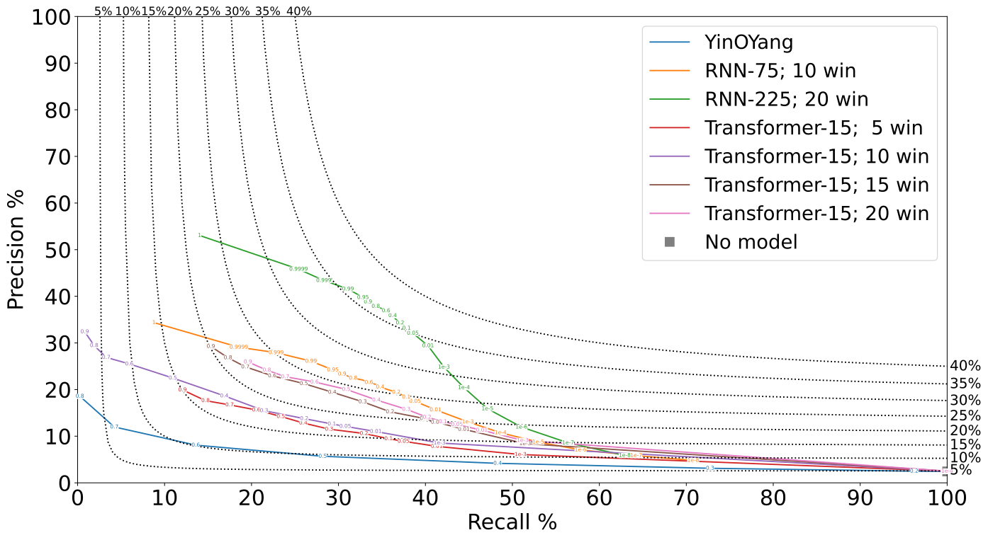
Metric Transformer-15; 5 win (This Work) Transformer-15; 10 win (This Work) Transformer-15; 15 win (This Work) Best Threshold 0.60 0.20 0.50 Recall (%) 20.54 26.06 26.02 Precision (%) 15.63 13.77 21.28 F₁ Score (%) 17.75 18.02 23.41 MCC (%) 15.50 16.08 21.36

Metric Transformer-15; 20 win (This Work) RNN-225; 20 win (Seber & Braatz (2023b)) YinOYang (Gupta & Brunak (2002)) No Model Best Threshold 0.50 0.60 0.60 N/A Recall (%) 30.89 35.47 13.59 100 Precision (%) 20.04 36.90 8.08 2.44 F₁ Score (%) 24.31 36.17 10.13 4.76 MCC (%) 22.49 34.57 7.57 0.00

A surprising result is how the performance of the transformer models does not change significantly with varying hyperparameters. Using large hidden sizes or adding another linear layer after the encoders slightly degrades the performance, while increasing the number of attention heads (to 4–5) and the number of stacked encoder layers (to 4) marginally improves the model. The most surprising result is the lack of significant improvement with increasing window size. As in Seber & Braatz (2023b), our models perform better with larger window sizes for sizes up to 20 (Fig. 1 and Table 1). The performance of a transformer encoder with a window size = 5 is only marginally inferior to the RNN from Seber & Braatz (2023b) using the same window size. However, whereas the RNNs’ performances increase quite significantly with increasing window size, the performance of the transformers barely improves. The only significant performance increase comes from increasing the window size from 10 to 15, but barely any performance is gained from further increasing this window size to 20 (Fig. 1).

3.2 The weighted focal differentiable MCC loss function is a superior alternative to the weighted CE

We hypothesized that changing the loss function can lead to improvements in the models’ metrics, as the weighted CE is optimizing a function that is only correlated with F₁ scores and MCC. Four other loss functions (as described in Section 2.4) are also used to cross-validate transformer models through the same procedure used with the weighted CE function (Sections 2.2 and 3.1).

The Focal, Lovász, and differentiable F₁ losses fail to achieve meaningful results. In the best-case scenarios, models trained with these loss functions can achieve F₁ scores equal to or slightly above 4.74%, equivalent to treating all (or almost all) sequences as positive. The differentiable F₁, in particular, frequently gets stuck at this local F₁ maximum. Naturally, these models have an MCC $\approx 0$ , as they are no better than random classifiers.

Conversely, the weighted focal differentiable MCC loss is able to attain very good performance on this problem (Fig. 2 and Table 2). For both architectures, its performance is superior to that of the weighted cross-entropy loss. As in Section 3.1, RNNs are considerably better than transformer encoders in predicting O-GlcNAcylation. The RNN model trained with the weighted focal differentiable MCC loss achieves an F₁ score = 37.03% and an MCC = 36.58%. The relative and absolute increases in MCC are higher than those for the F₁ score, highlighting the effectiveness of the weighted focal differentiable MCC loss, as it seeks to directly optimize the MCC. The weighted focal differentiable MCC loss can also be used for fine tuning; an RNN model first trained using weighted cross-entropy, then fine-tuned using the weighted focal differentiable MCC is generated (“RNN-225; CE $\rightarrow$ diff MCC”). This model initially followed the optimal hyperparameters (including model size) found through cross-validation using the weighted cross-entropy loss, but the learning rate and loss hyperparameters are changed to the optimal values found through cross-validation with the weighted focal differentiable MCC loss function when that loss function is used for fine-tuning. This fine-tuning also leads to a model that is better than the previous state-of-the-art from Seber & Braatz (2023b) (Fig. 2 and Table 2), reaching an F₁ score = 36.52% and an MCC = 36.01%, values slightly lower than that of the model trained only with the weighted focal differentiable MCC loss.

There is a significant difference between the optimal hyperparameters selected through the weighted cross-entropy and weighted focal differentiable MCC loss functions. Compared to the optimal values found through the weighted cross-entropy loss, the weighted focal differentiable MCC loss has an optimum at higher model hidden sizes (15 vs. 240 for transformers; 225 vs. 1425 for RNNs), higher batch sizes (256 vs. 512 for transformers; 32 vs. 128 for RNNs), lower learning rates (1 $\times 10^{-3}$ vs. 1 $\times 10^{-4}$ ), and lower class weights (15 vs. 3 for transformers; 30 vs. 3 for RNNs).

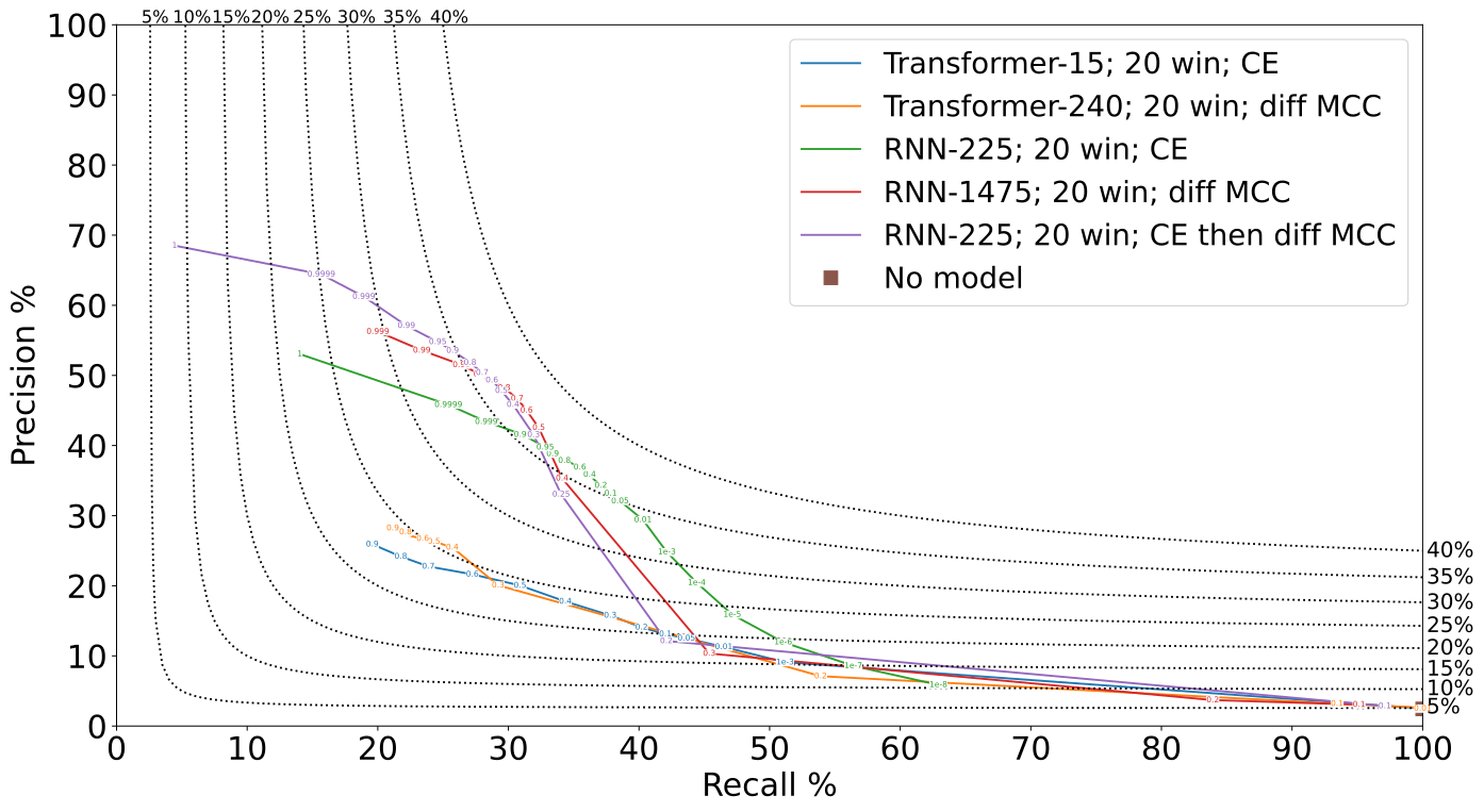
Table 2: Recall, precision, F₁ score, and MCC metrics (in %) for the highest F₁ score point of models tested on the modified dataset of Wulff-Fuentes et al. (2021). Model “RNN-225; CE” comes from Seber & Braatz (2023b). All others come from this work. The number after each RNN model is the LSTM module size used; the number after each transformer model is the hidden size used; the number after the semicolon for both types of models represents the window size on each side of the central S/T. “CE” represents the weighted cross-entropy loss, and “diff MCC” represents the weighted focal differentiable MCC loss. “No Model” sets all sites to potentially positive – that is, sets the threshold to 0.

Metric Transformer-15; CE (This Work) Transformer-240; diff MCC (This Work) RNN-225; CE (from Seber & Braatz (2023b)) Best Threshold 0.50 0.40 0.60 Recall (%) 30.89 25.70 35.47 Precision (%) 20.04 25.48 36.90 F₁ Score (%) 24.31 25.59 36.17 MCC (%) 22.49 23.67 34.57

Metric RNN-1425; diff MCC (This Work) RNN-225; CE $\rightarrow$ diff MCC (This Work) No Model Best Threshold 0.70 0.40 N/A Recall (%) 30.67 30.35 100 Precision (%) 46.70 45.84 2.44 F₁ Score (%) 37.03 36.52 4.76 MCC (%) 36.58 36.01 0.00

3.3 Two stacked RNNs provide better performance, and the weighted focal differentiable MCC loss is still superior

Seber & Braatz (2023b) trained RNNs with only a single cell, a restriction that was followed by this work in Section 3.2. However, RNNs with multiple stacked cells may perform better than single-cell RNNs. To verify this hypothesis, RNN models with 2 and 3 layers are tested (as per Section 2.3). Similarly to Section 3.2, three models are created: one trained only with the weighted CE loss, one trained only with the weighted focal differentiable MCC loss, and one first trained with the weighted CE loss, then fine-tuned with the weighted focal differentiable MCC loss. These models all surpass their single-RNN layer equivalents from Section 3.2. The model trained with the weighted CE loss (“RNN-[450,75]; CE”) displays the greatest relative improvement over its single-cell version, reaching an F₁ score = 38.73 % and an MCC = 37.31%. Like with the single-cell RNNs, fine-tuning with the weighted focal differentiable MCC loss after training with the weighted CE leads to improvements in the model performance; this fine-tuned model (“RNN-[450,75]; CE $\rightarrow$ diff MCC”) reaches an F₁ score = 38.83% and an MCC = 37.33%. While the performance improvement of fine-tuning is smaller in this scenario, these improved results again confirm the efficacy of fine-tuning with the weighted focal differentiable MCC loss. Finally, a model trained directly with the weighted focal differentiable MCC loss (“RNN-[600,75]; diff MCC”) achieves the best results, reaching an F₁ score = 38.82% and an MCC = 38.21%. The increase in MCC is considerably higher, further corroborating the benefits of this new loss function discussed in Section 3.2. Overall, the “RNN-[600,75]; diff MCC” model displays a 7.3% increase in F₁ score and a 10.5% increase in MCC over the “RNN-255; CE” model of Seber & Braatz (2023b).

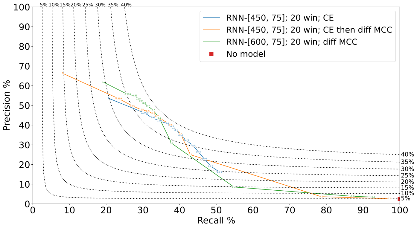
Table 3: Recall, precision, F₁ score, and MCC metrics (in %) for the highest F₁ score point of two-layer models tested on the modified dataset of Wulff-Fuentes et al. (2021). The number after each RNN model is the LSTM module size used, and the number after the semicolon represents the window size on each side of the central S/T. “CE” represents the weighted cross-entropy loss, and “diff MCC” represents the weighted focal differentiable MCC loss. The “No Model” (threshold = 0) baseline metrics are as in Tables 1 and 2.

Metric RNN-[450,75]; CE (This Work) RNN-[450,75]; CE $\rightarrow$ diff MCC (This Work) RNN-[600,75]; diff MCC (This Work) Best Threshold 0.90 0.50 0.60 Recall (%) 36.69 37.62 32.86 Precision (%) 41.02 40.11 47.44 F₁ Score (%) 38.73 38.83 38.82 MCC (%) 37.31 37.33 38.21

The models with the highest average cross-validation F₁ score all had two stacked RNN layers. Moreover, the optimal hidden size of the second RNN layer was always 75. As in Section 3.2, the optimal hyperparameters for models trained with the weighted focal differentiable MCC loss included higher model hidden sizes (450 vs. 600), lower learning rates (1 $\times 10^{-3}$ vs. 5 $\times 10^{-4}$ ), and lower class weights (20 vs. 2). Surprisingly, both models had the same optimal batch size (128), and the hidden size and class weights for the model trained with the weighted CE loss moved towards those from the model trained with the weighted focal differentiable MCC loss.

4 Discussion

This work generates transformer encoder (Section 3.1) and RNN (Sections 3.2 and 3.3) models to predict O-GlcNAcylation sites based on protein sequences using a modified version of an extensive public dataset (Wulff-Fuentes et al., 2021). These models are also compared to the state-of-the-art RNNs trained by Seber & Braatz (2023b).

While transformer models attain high performances on this dataset, they are inferior to the RNN models trained by Seber & Braatz (2023b), reaching an F₁ score of 24.31% and an MCC of 22.49% (Section 3.1, Fig. 1, and Table 1). A significant difference between transformers and RNNs is that the former do not scale well with increasing window sizes, while the latter display significant improvements with larger window sizes. With window size = 5, both transformers and RNNs possess similar performances, but a large performance gap arises with increasing window sizes.

Because the weighted cross-entropy loss function, which is used to train the models in Seber & Braatz (2023b) and Section 3.1 of this work, only indirectly optimizes the classification performance metrics, we hypothesized that a function that could directly improve the F₁ score and MCC can lead to better-performing models.

We develop the weighted focal differentiable MCC loss to address this question (Section 2.4; Algorithm 1). This function allows the direct optimization of the MCC, yielding better classification models. We cross-validate and test transformer and RNN models using the same dataset and notice that the performance of the weighted focal differentiable MCC loss is similar to but higher than that of the weighted cross-entropy loss (Section 3.2, Fig. 2, and Table 1). This loss function improves both the transformer and RNN architectures, and leads to the creation of an improved model with an F₁ score = 37.03% and an MCC = 36.58%. Furthermore, a model first trained using the weighted cross-entropy loss, then fine-tuned using the weighted focal differentiable MCC loss achieves improved performance in this prediction task relative to a model trained using only the weighted CE loss, reaching an F₁ score = 36.52% and an MCC = 36.01%. While these metrics are slightly smaller than the values obtained by a model directly trained with the weighted focal differentiable MCC loss, these results show how this new loss function can also be used to optimize and improve trained models at a low cost. The optimal hyperparameters for models trained with the weighted focal differentiable MCC loss are different from those of models trained with the weighted cross-entropy loss.

Because Seber & Braatz (2023b) used only single-cell models in their work, the RNN models from Section 3.2 follow this restriction. As models with multiple stacked cells can have better performance, we then train RNN models with more than one RNN cell in Section 3.3. Models with two stacked cells display superior cross-validation F₁ scores over models with one or three cells, and the best two-cell models have only 75 neurons in their 2nd cell. No matter the loss function used, these two-cell models display better performance in the test set than the RNN of Seber & Braatz (2023b) (Fig. 3 and Table 3). As in Section 3.2, fine-tuning using the weighted focal differentiable MCC loss after training with the weighted CE leads to improvements in performance over the model trained only with the weighted CE, corroborating one of the benefits of the weighted focal differentiable MCC loss. The model trained solely with the weighted focal differentiable MCC loss, “RNN-[600,75]; diff MCC”, achieves state-of-the-art performance in O-GlcNAcylation prediction, reaching an F₁ score = 38.82% and an MCC = 38.21%. Overall, this is a 7.3% increase in F₁ score and a 10.5% increase in MCC over the “RNN-255; CE” model of Seber & Braatz (2023b).

The code used in this work is publicly available, allowing the reproduction, improvement, and reuse of this work. It is simple to install and run the best RNN model to predict O-GlcNAcylation sites based on the local protein sequence. Instructions are provided in Sections A1.1 and A1.2 of the supplemental data or the README in our GitHub repository.

Impact statement

The first main benefit of this work is increasing the understanding of and prediction capability for O-GlcNAcylation, which will benefit fundamental research in cell and molecular biology and may lead to improvements in biopharmaceuticals or the creation of novel drugs. The second main benefit is the creation of the weighted focal differentiable MCC loss, a new loss function for classification tasks. This novel function can improve the performance of models and can even be used to fine-tune already trained models. Further work, especially work using different types of data and data from multiple fields, is necessary to corroborate the advantages of this novel loss function.

References

Abhishek & Hamarneh (2021) Abhishek, K. and Hamarneh, G. Matthews correlation coefficient loss for deep convolutional networks: Application to skin lesion segmentation. In 2021 IEEE 18th International Symposium on Biomedical Imaging (ISBI), pp. 225–229, 2021. URL https://doi.org/10.1109/ISBI48211.2021.9433782.
Ahmed & Cheung (2014) Ahmed, M. and Cheung, N.-K. V. Engineering anti-GD2 monoclonal antibodies for cancer immunotherapy. FEBS Letters, 588(2):288–297, 2014. URL https://doi.org/10.1016/j.febslet.2013.11.030.
Almeida & Kolarich (2016) Almeida, A. and Kolarich, D. The promise of protein glycosylation for personalised medicine. Biochimica et Biophysica Acta (BBA) - General Subjects, 1860(8):1583–1595, 2016. URL https://doi.org/10.1016/j.bbagen.2016.03.012.
Berman et al. (2018) Berman, M., Triki, A. R., and Blaschko, M. B. The lovasz-softmax loss: A tractable surrogate for the optimization of the intersection-over-union measure in neural networks. In 2018 IEEE/CVF Conference on Computer Vision and Pattern Recognition, pp. 4413–4421, 2018. URL https://doi.org/10.1109/CVPR.2018.00464.
Bhat et al. (2019) Bhat, A. H., Maity, S., Giri, K., and Ambatipudi, K. Protein glycosylation: Sweet or bitter for bacterial pathogens? Critical Reviews in Microbiology, 45(1):82–102, 2019. URL https://doi.org/10.1080/1040841X.2018.1547681.
Bénédict et al. (2022) Bénédict, G., Koops, V., Odijk, D., and de Rijke, M. sigmoidF₁: A smooth F₁ score surrogate loss for multilabel classification, 2022. URL https://arxiv.org/abs/2108.10566.
Chang et al. (2020) Chang, Y.-H., Weng, C.-L., and Lin, K.-I. O-GlcNAcylation and its role in the immune system. Journal of Biomedical Science, 27(1):57, 2020. URL https://doi.org/10.1186/s12929-020-00648-9.
Gonzalez & Miikkulainen (2020) Gonzalez, S. and Miikkulainen, R. Improved training speed, accuracy, and data utilization through loss function optimization. In 2020 IEEE Congress on Evolutionary Computation (CEC), pp. 1–8, 2020. URL https://doi.org/10.1109/CEC48606.2020.9185777.
Gupta & Brunak (2002) Gupta, R. and Brunak, S. Prediction of glycosylation across the human proteome and the correlation to protein function. Pacific Symposium on Biocomputing, pp. 310–22, 2002.
Harris et al. (2020) Harris, C. R., Millman, K. J., van der Walt, S. J., Gommers, R., Virtanen, P., Cournapeau, D., Wieser, E., Taylor, J., Berg, S., Smith, N. J., Kern, R., Picus, M., Hoyer, S., van Kerkwijk, M. H., Brett, M., Haldane, A., del Río, J. F., Wiebe, M., Peterson, P., Gérard-Marchant, P., Sheppard, K., Reddy, T., Weckesser, W., Abbasi, H., Gohlke, C., and Oliphant, T. E. Array programming with NumPy. Nature, 585(7825):357–362, September 2020. URL https://doi.org/10.1038/s41586-020-2649-2.
Ho et al. (2016) Ho, W.-L., Hsu, W.-M., Huang, M.-C., Kadomatsu, K., and Nakagawara, A. Protein glycosylation in cancers and its potential therapeutic applications in neuroblastoma. Journal of Hematology & Oncology, 9(1):100, 2016. URL https://doi.org/10.1186/s13045-016-0334-6.
Hokke et al. (1995) Hokke, C. H., Bergwerff, A. A., Dedem, G. W. K., Kamerling, J. P., and Vliegenthart, J. F. G. Structural analysis of the sialylated N- and O-linked carbohydrate chains of recombinant human erythropoietin expressed in Chinese hamster ovary cells. Sialylation patterns and branch location of dimeric N-acetyllactosamine units. European Journal of Biochemistry, 228(3):981–1008, 1995. URL https://doi.org/10.1111/j.1432-1033.1995.0981m.x.
Ilievski & Feng (2017) Ilievski, I. and Feng, J. A simple loss function for improving the convergence and accuracy of visual question answering models, 2017. URL https://arxiv.org/abs/1708.00584.
Jaeken (2013) Jaeken, J. Chapter 179 – congenital disorders of glycosylation. In Dulac, O., Lassonde, M., and Sarnat, H. B. (eds.), Pediatric Neurology Part III, volume 113 of Handbook of Clinical Neurology, pp. 1737–1743. Elsevier, Amsterdam, 2013. URL https://doi.org/10.1016/B978-0-444-59565-2.00044-7.
Jia et al. (2018) Jia, C., Zuo, Y., and Zou, Q. O-GlcNAcPRED-II: an integrated classification algorithm for identifying O-GlcNAcylation sites based on fuzzy undersampling and a K-means PCA oversampling technique. Bioinformatics, 34(12):2029–2036, 2018. URL https://doi.org/10.1093/bioinformatics/bty039.
Kukleva et al. (2023) Kukleva, A., Böhle, M., Schiele, B., Kuehne, H., and Rupprecht, C. Temperature schedules for self-supervised contrastive methods on long-tail data. arXiv:2303.13664, 2023. URL https://doi.org/10.48550/arXiv.2303.13664.
Lee et al. (2021) Lee, N., Yang, H., and Yoo, H. A surrogate loss function for optimization of $f_{\beta}$ score in binary classification with imbalanced data, 2021. URL https://doi.org/10.48550/arXiv.2104.01459.
Lin et al. (2017) Lin, T., Goyal, P., Girshick, R. B., He, K., and Dollár, P. Focal loss for dense object detection. CoRR, abs/1708.02002, 2017. URL http://arxiv.org/abs/1708.02002.
Loshchilov & Hutter (2017) Loshchilov, I. and Hutter, F. SGDR: Stochastic gradient descent with warm restarts. arXiv:1608.03983, 2017. URL https://doi.org/10.48550/arXiv.1608.03983.
Mauri et al. (2021) Mauri, T., Menu-Bouaouiche, L., Bardor, M., Lefebvre, T., Lensink, M. F., and Brysbaert, G. O-GlcNAcylation prediction: An unattained objective. Advances and Applications in Bioinformatics and Chemistry, Volume 14:87–102, 2021. URL https://doi.org/10.2147/AABC.S294867.
McKinney (2010) McKinney, W. Data structures for statistical computing in Python. In van der Walt, S. and Millman, J. (eds.), Proceedings of the 9th Python in Science Conference, pp. 56–61, 2010. URL https://doi.org/10.25080/Majora-92bf1922-00a.
Mishra et al. (2019) Mishra, S., Yamasaki, T., and Imaizumi, H. Improving image classifiers for small datasets by learning rate adaptations. In 2019 16th International Conference on Machine Vision Applications (MVA), pp. 1–6, 2019. URL https://doi.org/10.23919/MVA.2019.8757890.
Moon et al. (2021) Moon, S., Chatterjee, S., Seeberger, P. H., and Gilmore, K. Predicting glycosylation stereoselectivity using machine learning. Chemical Science, 12(8):2931–2939, 2021. URL https://doi.org/10.1039/D0SC06222G.
Padler-Karavani et al. (2008) Padler-Karavani, V., Yu, H., Cao, H., Chokhawala, H., Karp, F., Varki, N., Chen, X., and Varki, A. Diversity in specificity, abundance, and composition of anti-Neu5Gc antibodies in normal humans: Potential implications for disease. Glycobiology, 18(10):818–830, 2008. URL https://doi.org/10.1093/glycob/cwn072.
Paszke et al. (2019) Paszke, A., Gross, S., Massa, F., Lerer, A., Bradbury, J., Chanan, G., Killeen, T., Lin, Z., Gimelshein, N., Antiga, L., Desmaison, A., Kopf, A., Yang, E., DeVito, Z., Raison, M., Tejani, A., Chilamkurthy, S., Steiner, B., Fang, L., Bai, J., and Chintala, S. PyTorch: An imperative style, high-performance deep learning library. In Advances in Neural Information Processing Systems 32, pp. 8024–8035. Curran Associates, Inc., 2019. URL http://papers.neurips.cc/paper/9015-pytorch-an-imperative-style-high-performance-deep-learning-library.pdf.
Pedregosa et al. (2011) Pedregosa, F., Varoquaux, G., Gramfort, A., Michel, V., Thirion, B., Grisel, O., Blondel, M., Prettenhofer, P., Weiss, R., Dubourg, V., Vanderplas, J., Passos, A., Cournapeau, D., Brucher, M., Perrot, M., and Duchesnay, E. Scikit-learn: Machine learning in Python. Journal of Machine Learning Research, 12:2825–2830, 2011.
Schjoldager et al. (2020) Schjoldager, K. T., Narimatsu, Y., Joshi, H. J., and Clausen, H. Global view of human protein glycosylation pathways and functions. Nature Reviews Molecular Cell Biology, 21(12):729–749, 2020. URL https://doi.org/10.1038/s41580-020-00294-x.
Seber & Braatz (2023a) Seber, P. and Braatz, R. D. Linear and neural network models for predicting N-glycosylation in Chinese Hamster Ovary cells based on B4GALT levels. bioRxiv, 2023a. URL https://doi.org/10.1101/2023.04.13.536762.
Seber & Braatz (2023b) Seber, P. and Braatz, R. D. Recurrent neural network-based prediction of O-GlcNAcylation sites in mammalian proteins. bioRxiv, 2023b. URL https://doi.org/10.1101/2023.08.24.554563.
Shapley (1951) Shapley, L. S. Notes on the n-person game – II: The value of an n-person game. U.S. Air Force Project RAND, 8 1951.
Stowell et al. (2015) Stowell, S. R., Ju, T., and Cummings, R. D. Protein glycosylation in cancer. Annual Review of Pathology: Mechanisms of Disease, 10(1):473–510, 2015. URL https://doi.org/10.1146/annurev-pathol-012414-040438.
Van Landuyt et al. (2019) Van Landuyt, L., Lonigro, C., Meuris, L., and Callewaert, N. Customized protein glycosylation to improve biopharmaceutical function and targeting. Current Opinion in Biotechnology, 60:17–28, 2019. URL https://doi.org/10.1016/j.copbio.2018.11.017.
Wulff-Fuentes et al. (2021) Wulff-Fuentes, E., Berendt, R. R., Massman, L., Danner, L., Malard, F., Vora, J., Kahsay, R., and Stichelen, S. O.-V. The human O-GlcNAcome database and meta-analysis. Scientific Data, 8(1):25, 2021. URL https://doi.org/10.1038/s41597-021-00810-4.
Zhu & Hart (2021) Zhu, Y. and Hart, G. W. Targeting O-GlcNAcylation to develop novel therapeutics. Molecular Aspects of Medicine, 79:100885, 2021. URL https://doi.org/10.1016/j.mam.2020.100885.

A1 Appendix

A1.1 Reproducing the models and plots

The transformer models can be recreated by downloading the datasets and running the transformer_train.py file with the appropriate flags (run python transformer_train.py --help for details).

The RNN models can be recreated by downloading the datasets and running the ANN_train.py file with the appropriate flags (run python ANN_train.py --help for details).

The plots can be recreated by running the make_plot.py file with the appropriate flag as an input (python make_plot.py ce for Fig. 1, python make_plot.py diffMCC for Fig. 2, and python make_plot.py multilayer for Fig. 3).

A1.2 Using the RNN model to predict O-GlcNAcylation sites

The Conda environment defining the specific packages and version numbers used in this work is available as ANN_environment.yaml on our GitHub <redacted for review>. To use our trained model, run the Predict.py file as python Predict.py <sequence> -t <threshold> -bs <batch_size>.

Alternatively, create an (N+1)x1 .csv with the first row as a header (such as "Sequences") and all other N rows as the actual amino acid sequences, then run the Predict.py file as python Predict.py <path/to/file.csv> -t <threshold> -bs <batch_size>. Results are saved as a new .csv file.