Design principles of nonlinear optical materials for Terahertz lasers

Abstract

We have investigated both inter-band and intra-band second order nonlinear optical conductivity based on the velocity correlation formalism and the spectral expansion technique. We propose a scenario in which the second order intra-band process is nonzero while the inter-band process is zero. This occurs for a band structure with momentum asymmetry in the Brillouin zone. Very low-energy photons are blocked by the Pauli exclusion principle from participating in the inter-band process; however, they are permitted to participate in the intra-band process, with the band smeared by some impurity scattering. We establish a connection between the inter-band nonlinear optical conductivity in the velocity gauge and the shift vector in the length gauge for a two-band model. Using a quasiclassical kinetic approach, we demonstrate the importance of intra-band transitions in high harmonic generations for the single tilted Dirac cone model and hexagonal warping model. We confirm that the Kramers-Kronig relations break down for the limit case of ($\omega$, $-\omega$) in the nonlinear optical conductivity. Finally, we calculate the superconducting transition temperature of NbN and the dielectric function of AlN, and the resistance of the NbN/AlN junction. The natural non-linearity of the Josephson junction brings a Josephson plasma with frequency in the Terahertz region.

Nonlinear phenomena are widely used in the design of Terahertz (0.1 THz to 10 THz, less investigated in the whole electromagnetic spectrum and termed as the “THz gap”) laser sources. For example, up-conversion from microwave GHz using the step recovery diode, is based on the nonlinear sum-frequency mixing. While down-conversion from the visible and ultraviolet is based on the nonlinear difference-frequency mixing, also used to detect electromagnetic radiations by the electro-optic sampling [1, 2]. The efficiency of THz-pulse generation was further improved by the velocity matching from the pulse front tilting [3].

The requirement of broadband THz sources and detectors suggests the use of materials with second-order optical nonlinearities. Recently, high-efficiency solar energy harvesting was discovered in non-centrosymmetric crystal structures such as Bismuth ferrites, perovskite oxides, ferroelectric materials and topological insulators [4, 5, 6, 7, 8, 9, 10, 11]. The nonlinear photovoltaics in non-centrosymmetric crystals is also termed as shift current photovoltaics [4, 11]. The nonlinear current is connected to a shift vector, which is the subtraction of the Berry connection of the conduction and the valence band. The Berry connection is an expectation value of the position operator, and its curl is the Berry curvature, related to topological quantities of the material.

A typical second-order nonlinear process was first demonstrated by projecting a laser beam with frequency $\omega$ through crystalline quartz [12] to generate a laser beam with frequency $2\omega$. Later on the second-harmonic generation (SHG) was found in other materials (e.g., silicon surfaces) [13] with broken inversion symmetry. Nonlinear optical analogs, including SHG, have also been studied recently in various contexts, including Josephson plasma waves [14] and cavity quantum electrodynamics [15, 16, 17, 18]. Theoretically, the nonlinear susceptibility tensor was used to describe the nonlinear electrical current in response to the external electric field, in semiconductors [19], and single-layer graphene [20, 21] with oblique incidence of radiation on the 2D electron layer. In the long-wavelength limit (the wave vector $\mathbf{q}\rightarrow 0$, normal incidence), the nonlinear optical conductivity vanishes for materials with inversion symmetry.

Nonlinear susceptibility $\chi$ appears in the relation of nonlinear polarization $P$ and the electric field $E$, $P_{\alpha}(\omega_{1}+\omega_{2})=\chi_{\alpha\beta\gamma}(\omega_{1}+\omega_{2})E_{\beta}(\omega_{1})E_{\gamma}(\omega_{2})$. The electric current $J(t)$ and the polarization is connected by $J(t)=dP(t)/dt$. The nonlinear conductivity $\tilde{\sigma}$ connects the electric current and the electric field, $J_{\alpha}(\omega_{1}+\omega_{2})=\tilde{\sigma}_{\alpha\beta\gamma}(\omega_{1}+\omega_{2})E_{\beta}(\omega_{1})E_{\gamma}(\omega_{2})$. It is obtained from two approaches, the velocity operator approach [22], Eq. (2-48) and Eq. (2-49); and the position operator approach [4, 5, 10]. To establish the connection between velocity-operator approach and postion-operator approach, we start from a two-band model. For example, the Hamiltonian $H_{0}$, eigenstates $u(\mathbf{k},s)$ and the corresponding eigenvalues $\varepsilon_{s}(\mathbf{k})$ are defined in the equation $H_{0}u(\mathbf{k},s)=\varepsilon_{s}(\mathbf{k})u(\mathbf{k},s),$ where $s$ is the band index and $\mathbf{k}$ the momentum. The velocity operator matrix element is defined as $v_{s^{\prime}s}^{x(y)}=\langle s^{\prime}|\frac{\partial H_{0}}{\partial k_{x(y)}}|s\rangle$ where $u(\mathbf{k},s)$ is denoted by $|s\rangle$. The position operator matrix element is defined as $r_{s^{\prime}s}^{x(y)}=i\langle s^{\prime}|\frac{\partial}{\partial k_{x(y)}}|s\rangle$. Take a second derivative of the Hamiltonian matrix elements, we obtained,

$$\frac{\partial}{\partial k_{\alpha}}\frac{\partial}{\partial k_{\beta}}\langle s^{\prime}|H_{0}|s\rangle=\delta_{ss^{\prime}}\frac{\partial}{\partial k_{\alpha}}\frac{\partial}{\partial k_{\beta}}\varepsilon_{s}(\mathbf{k})\,.$$

The $x$ and $y$ component of the shift vector $R$ is defined as

$$R_{s^{\prime}s}^{x(y)}=\frac{i\partial}{\partial k_{x(y)}}+i\langle s^{\prime}|\frac{\partial s^{\prime}}{\partial k_{x(y)}}\rangle-i\langle s|\frac{\partial s}{\partial k_{x(y)}}\rangle\,,$$

If the particle-hole symmetry is preserved, we have $\varepsilon_{+}(\mathbf{k})=-\varepsilon_{-}(\mathbf{k})=E$ and $v_{++}^{x}=-v_{--}^{x}$. As shown in the supplementary material[23], velocity matrix elements are connected with position matrix elements and shift vectors in the following equations, for $\tilde{\sigma}_{xxx}$ the equation is

$$v_{+-}^{x}v_{++}^{x}v_{-+}^{x}=2iE^{3}r_{+-}^{x}R_{-+}^{x}r_{-+}^{x}+ir_{+-}^{x}\tilde{m}_{-+}^{xx}\,,$$ (1)

where $\tilde{m}_{ss^{\prime}}^{\alpha\beta}=E^{2}\langle s|\frac{\partial^{2}H_{0}}{\partial k_{\alpha}\partial k_{\beta}}|s^{\prime}\rangle$ is proportional to the inverse of the effective mass defined from the band curvature. For a flat band, the second term in Eq. [1] vanishes, the shift vector approach is the same as the velocity approach. However, this conclusion is only valid for the inter-band nonlinear optical conductivity. In below, we develop a theory to consider both the intra-band and the inter-band nonlinear optical conductivity.

For the linear conductivity, it is well known a trace of velocity operators and Green’s functions is connected to the product of velocity matrix elements. We now define the nonlinear conductivity as a trace of velocity operators and Green’s functions [24]; the momentum and imaginary frequency parameters in each Green’s function is set by using a triangle Feynman diagram,

$$\tilde{\sigma}_{\alpha\beta\gamma}(\omega_{a},\omega_{b})=\frac{ie^{3}}{\omega_{a}\omega_{b}}\int d\mathbf{k}T\sum_{l}\mathrm{Tr}\langle v_{\alpha}\widehat{G}(\mathbf{k,}i\omega_{l})v_{\beta}\times$$

$$\widehat{G}(\mathbf{k,}i\omega_{l}+i\omega_{n1})v_{\gamma}\widehat{G}(\mathbf{k,}i\omega_{l}-i\omega_{n2})\rangle_{i\omega_{n1(2)}\rightarrow\omega_{a(b)}+i\delta}\,.$$ (2)

Here $e$ is the charge of the electron, $T$ is the temperature with $\omega_{n1,2}$ = 2n$\pi$$T$ , $\omega_{l}=(2l+1)$$\pi$$T$ the Boson and Fermion Matsubara frequencies, $n$ and $l$ are integers and $T_{r}$ is a trace, $\int d\mathbf{k}=\int dk_{x}/$(2$\pi$) for one-dimension(1D) and $\int d\mathbf{k}=\int dk_{x}dk_{y}/(4{\pi^{2}}$) for two-dimension(2D). For simplicity we set $\hbar$ = 1, $c$ = 1 and $k_{B}$ = 1. To obtain the nonlinear conductivity, which is a real frequency quantity, we need to make an analytic continuation from imaginary $i\omega_{n}$ to real $\omega$ and $\delta$ is infinitesimal. The matrix Green’s function $\widehat{G}(\mathbf{k,}i\omega_{l})$ could be obtained from the spectral function, which is directly measured in the angular resolved photoemission spectroscopy (ARPES) experiment; or from theoretical evaluation of the self energy $\sum(\mathbf{k,}i\omega_{l})$ , which has contributions from electron-electron, electron-phonon scattering or disorder scattering. Theoretically the Green’s function is obtained from $\widehat{G}^{-1}(\mathbf{k,}i\omega_{l})=\widehat{G}_{0}^{-1}(\mathbf{k,}i\omega_{l})+\sum(\mathbf{k,}i\omega_{l})$, where $\widehat{G}_{0}(\mathbf{k,}i\omega_{l})$ is the free electron Green’s function satisfying $\widehat{G}_{0}^{-1}(\mathbf{k,}i\omega_{l})=i\omega_{l}-H_{0}(\mathbf{k})$.

The matrix Green’s function $\widehat{G}(\mathbf{k},i\omega_{l})$ can be conveniently written in terms of a matrix spectral function $\widehat{A}(\mathbf{k},\omega)$ with

$$\widehat{G}(\mathbf{k},i\omega_{l})=\int_{-\infty}^{\infty}\frac{d\omega}{2\pi}\frac{\widehat{A}(\mathbf{k},\omega)}{i\omega_{l}-\omega}\,,$$ (3)

then the conductivity becomes

$$\tilde{\sigma}_{\alpha\beta\gamma}=\frac{ie^{3}}{\omega_{a}\omega_{b}}\int A(\mathbf{k})B(\omega_{n1,2})_{i\omega_{n1(2)}\rightarrow\omega_{a(b)}+i\delta}$$ (4)

here the integrals are $\int=\int d\mathbf{k}\int d\omega_{1,2,3}$ where $\int d\omega_{1,2,3}=\int_{-\infty}^{\infty}\frac{d\omega_{1}}{2\pi}\int_{-\infty}^{\infty}\frac{d\omega_{2}}{2\pi}\int_{-\infty}^{\infty}\frac{d\omega_{3}}{2\pi}$. We have defined two functions

$$A(\mathbf{k})=\mathrm{Tr}\langle v_{\alpha}\widehat{A}(\mathbf{k,}\omega_{1})v_{\beta}\widehat{A}(\mathbf{k,}\omega_{2})v_{\gamma}\widehat{A}(\mathbf{k,}\omega_{3})\rangle$$ (5)

which does not depend on $\omega_{n1,2}$ and

$$B(\omega_{n1,2})=T\sum_{l}\frac{1}{i\omega_{l}-\omega_{1}}\frac{1}{i\omega_{l}+i\omega_{n1}-\omega_{2}}\frac{1}{i\omega_{l}-i\omega_{n2}-\omega_{3}}$$ (6)

which does not depend on $\mathbf{k}$. Both of them depend on $\omega_{1,2,3}$. Performing the sum over Matsubara frequencies, with details in the supplementary, we obtain

$$B(\omega_{n1,2})=\frac{1}{i\omega_{n1}-\omega_{2}+\omega_{1}}$$ (7)

$$\times \Big{[}\frac{f(\omega_{3})-f(\omega_{1})}{i\omega_{n2}+\omega_{3}-\omega_{1}}+\frac{f(\omega_{2})-f(\omega_{3})}{i\omega_{n1}+i\omega_{n2}+\omega_{3}-\omega_{2}}\Big{]}\,.$$

Here $f(x)=1/[\exp(x/T-\mu/T)+1]$ is the Fermi-Dirac distribution function obtained from the sum over the internal Fermion Matsubara frequencies $\omega_{l}$. From Eqn. (3), we know $\widehat{A}(\mathbf{k,}\omega)=-2\rm{Im}\widehat{G}(\mathbf{k},\omega)$. For a two-band model, the free electron spectral function consists of delta-functions,

$$\widehat{A}(\mathbf{k,}\omega)=2\pi\delta(\omega+\mu-\varepsilon_{+})|+\rangle\langle+|+2\pi\delta(\omega+\mu-\varepsilon_{-})|-\rangle\langle-|$$

For $\alpha=x$ or $y$, $\beta=x$ and $\gamma=x$ the trace in $A(\mathbf{k})$ is carried out

$$A(\mathbf{k})=8\pi^{3}\Big{[}v_{++}^{x(y)}v_{++}^{x}v_{++}^{x}\delta_{+++}+v_{+-}^{x(y)}v_{--}^{x}v_{-+}^{x}\delta_{--+}$$

$$+v_{++}^{x(y)}v_{+-}^{x}v_{-+}^{x}\delta_{+-+}+v_{+-}^{x(y)}v_{-+}^{x}v_{++}^{x}\delta_{-++}$$

$$+v_{-+}^{x(y)}v_{++}^{x}v_{+-}^{x}\delta_{++-}+v_{--}^{x(y)}v_{--}^{x}v_{--}^{x}\delta_{---}$$

$$+v_{-+}^{x(y)}v_{+-}^{x}v_{--}^{x}\delta_{+--}+v_{--}^{x(y)}v_{-+}^{x}v_{+-}^{x}\delta_{-+-}\Big{]}$$ (8)

with the definition $\delta_{s_{1}s_{2}s_{3}}=$

$$\delta(\omega_{1}+\mu-\varepsilon_{s_{1}})\delta(\omega_{2}+\mu-\varepsilon_{s_{2}})\delta(\omega_{3}+\mu-\varepsilon_{s_{3}})$$

Now we separate the inter-band and intra-band process, $\tilde{\sigma}_{xxx}=\tilde{\sigma}^{\textrm{inter}}_{xxx}+\tilde{\sigma}^{\textrm{intra}}_{xxx}$, and $A(\mathbf{k})=A^{\textrm{inter}}(\mathbf{k})+A^{\textrm{intra}}(\mathbf{k})$. Collecting all the inter-band contributions for $\tilde{\sigma}^{\textrm{inter}}_{xxx}$ we have

$$A^{\textrm{inter}}(\mathbf{k}) = 8\pi^{3}v_{+-}^{x}v_{-+}^{x}\Big{[}v_{++}^{x}(\delta_{+-+}+\delta_{-++}+\delta_{++-})$$ (9)

$$+ v_{--}^{x}(\delta_{+--}+\delta_{-+-}+\delta_{--+})\Big{]}$$

Collecting all the intra-band contributions for $\tilde{\sigma}^{\textrm{intra}}_{xxx}$ we have

$$A^{\textrm{intra}}(\mathbf{k})=8\pi^{3}\Big{[}(v_{++}^{x})^{3}\delta_{+++}+(v_{--}^{x})^{3}\delta_{---}\Big{]}$$ (10)

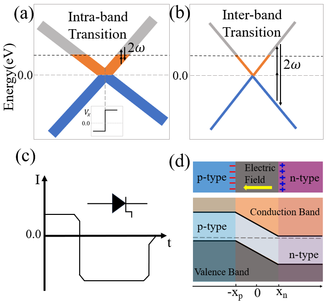
Figure 1: Schematic of (a) intra-band and (b) inter-band transition [25]. In the inset of (a), the velocity changes abruptly as a function of k. (c) Current and time relationship of the step recovery diode. The current changes abruptly as a function of t. (d) Schematic of a pn-junction and its energy band. From Poisson’s equation, the redistribution of the electric charge concentration in the pn-junction is connected to the strong internal electric field in materials, which is important to realize asymmetric energy as depicted in (a).

For the interband nonlinear conductivity, the delta functions $\delta_{s_{1}s_{2}s_{3}}$ could be used to carry out the integral $\int d\omega_{1,2,3}$. For nonequal frequencies $\omega_{a}$ and $\omega_{b}$, we have

$$\tilde{\sigma}_{xxx}^{\textrm{inter}}=\frac{ie^{3}}{\omega_{a}\omega_{b}}\int d\mathbf{k}\sum_{s=\pm}\Big{[}\sum_{n=a,b}\frac{f(\varepsilon_{-})-f(\varepsilon_{+})}{\omega_{a}+\omega_{b}+2i\delta+sp\varepsilon_{\Delta}}$$ (11)

$$\times \frac{sv_{+-}^{x}v_{-+}^{x}v^{x}_{ss}}{\omega_{n}+i\delta+sp\varepsilon_{\Delta}}+\frac{f(\varepsilon_{+})-f(\varepsilon_{-})}{\omega_{b}+i\delta+s\varepsilon_{\Delta}}\frac{sv_{+-}^{x}v_{-+}^{x}v^{x}_{ss}}{\omega_{a}+i\delta-s\varepsilon_{\Delta}}\Big{]}$$

where $\varepsilon_{\Delta}=\varepsilon_{+}-\varepsilon_{-}$, $p=+1$ for $n=a$ and $p=-1$ for $n=b$. Note that if the inversion symmetry was not broken, i.e. $v^{x}(\mathbf{k})v^{x}(\mathbf{k})v^{x}(\mathbf{k})=-v^{x}(-\mathbf{k})v^{x}(-\mathbf{k})v^{x}(-\mathbf{k})$, the integrand is an odd function of $\mathbf{k}$ so the integration in momentum space vanishes. For the intra-band nonlinear conductivity, the integral $\int d\omega_{1,2,3}$ is not integrated out and we use the same notation $\int=\int d\mathbf{k}\int d\omega_{1,2,3}$,

$$\tilde{\sigma}_{xxx}^{\textrm{intra}}=\frac{ie^{3}}{\omega_{a}\omega_{b}}\int\frac{A^{\textrm{intra}}(\mathbf{k})}{\omega_{a}+i\delta-\omega_{2}+\omega_{1}}\times$$

$$\Big{[}\frac{f(\omega_{3})-f(\omega_{1})}{\omega_{b}+i\delta+\omega_{3}-\omega_{1}}+\frac{f(\omega_{2})-f(\omega_{3})}{\omega_{a}+\omega_{b}+2i\delta+\omega_{3}-\omega_{2}}\Big{]}$$ (12)

Now we are ready to discuss two limit cases $\omega_{a}=\omega_{b}=\omega$ and $\omega_{a}=-\omega_{b}=\omega$, for the inter-band nonlinear optical conductivity we have

$$\tilde{\sigma}_{xxx}^{\textrm{inter}}(\omega,\omega)=\frac{ie^{3}}{\omega^{2}}\int d\mathbf{k}\frac{v_{+-}^{x}v_{-+}^{x}v^{x}_{\Delta}}{\varepsilon_{\Delta}}\times$$

$$\sum_{s=\pm}\Big{[}\frac{0.5s[f(\varepsilon_{+})-f(\varepsilon_{-})]}{\omega+i\delta+s\varepsilon_{\Delta}}+\frac{s[f(\varepsilon_{+})-f(\varepsilon_{-})]}{\omega+i\delta-0.5s\varepsilon_{\Delta}}\Big{]}.$$ (13)

where $v^{x}_{\Delta}=v_{++}^{x}-v_{--}^{x}$. However for the $\omega_{a}=-\omega_{b}=\omega$ case, the nonlinear conductivity is a pure imaginary number, as $\tilde{\sigma}_{xxx}^{\textrm{inter}}(\omega,-\omega)=$

$$\frac{ie^{3}}{\omega^{2}}\int d\mathbf{k}\sum_{s=\pm}sv_{+-}^{x}v_{-+}^{x}v^{x}_{ss}\Bigg{[}\frac{f(\varepsilon_{+})-f(\varepsilon_{-})}{(\omega-s\varepsilon_{\Delta})^{2}+\delta^{2}}$$

$$+\frac{2(\varepsilon^{2}_{\Delta}+s\omega\varepsilon_{\Delta}-2\delta^{2})[f(\varepsilon_{+})-f(\varepsilon_{-})]}{(\varepsilon^{2}_{\Delta}+s\omega\varepsilon_{\Delta}-2\delta^{2})^{2}+\delta^{2}(3s\varepsilon_{\Delta}+2\omega)^{2}}\Bigg{]}\,.$$ (14)

This breaks the Kramers-Kronig relation for the inter-band nonlinear optical conductivity. For the intra-band part, we do not use the free-electron spectral function, but keep the self-energy from the impurity scattering. So the delta function becomes a broadened Lorentzian $\delta(\omega_{1}+\mu-\varepsilon_{\pm})\rightarrow(-1/\pi)\rm{Im}[1/(\omega_{1}+i\delta+\mu-\varepsilon_{\pm})]=S_{\pm}(\omega_{1})$, for the $\omega_{a}=\omega_{b}=\omega$ case we have

$$\tilde{\sigma}_{xxx}^{\textrm{intra}}(\omega,\omega)=\frac{ie^{3}}{\omega^{2}}\int\frac{S(\omega_{1},\omega_{2},\omega_{3})}{\omega_{3}+\omega_{2}-2\omega_{1}}\Big{[}\frac{f(\omega_{2})-f(\omega_{1})}{\omega+i\delta-\omega_{2}+\omega_{1}}$$

$$+\frac{f(\omega_{1})-f(\omega_{3})}{\omega+i\delta+\omega_{3}-\omega_{1}}+\frac{f(\omega_{3})-f(\omega_{2})}{\omega+i\delta+0.5\omega_{3}-0.5\omega_{2}}\Big{]}\,,$$ (15)

where $S(\omega_{1},\omega_{2},\omega_{3})=8\pi^{3}[(v_{++}^{x})^{3}S_{+}(\omega_{1})S_{+}(\omega_{2})S_{+}(\omega_{3})+(v_{--}^{x})^{3}S_{-}(\omega_{1})S_{-}(\omega_{2})S_{-}(\omega_{3})]$. For the $\omega_{a}=-\omega_{b}=\omega$ case, $\tilde{\sigma}^{\textrm{intra}}_{xxx}(\omega,-\omega)=$

$$\frac{-ie^{3}}{\omega^{2}}\int\frac{S(\omega_{1},\omega_{2},\omega_{3})}{\omega_{3}+\omega_{2}-2\omega-2\omega_{1}}\Big{[}\frac{f(\omega_{3})-f(\omega_{2})}{i\delta+0.5(\omega_{3}-\omega_{2})}$$

$$+\frac{f(\omega_{1})-f(\omega_{3})}{-\omega+i\delta+\omega_{3}-\omega_{1}}+\frac{f(\omega_{2})-f(\omega_{1})}{\omega+i\delta-\omega_{2}+\omega_{1}}\Big{]}$$ (16)

If we focus on the real part of the nonlinear conductivity, the equation is further simplified, we reduce the three-dimenion integration over the frequency to a two-dimension one, which we numerically sovled in [26]

$$\ \rm{Re}\tilde{\sigma}^{\textrm{intra}}_{xxx}(\omega,\omega)=\frac{e^{3}}{2\omega^{2}}\int d\mathbf{k}\int d\omega_{1,2}\Big{[}S(\omega_{1},\omega_{2},\omega_{1}+\omega)\times$$

$$\ \frac{f(\omega_{1}+\omega)-f(\omega_{1})}{\omega_{2}-\omega_{1}+\omega}+S(\omega_{1},\omega_{2},\omega_{1}-\omega)\frac{f(\omega_{1})-f(\omega_{1}-\omega)}{\omega_{2}-\omega_{1}-\omega}$$

$$\ +S(\omega_{1},\omega_{2},\omega_{2}-2\omega)\frac{f(\omega_{2}-2\omega)-f(\omega_{2})}{\omega_{2}-\omega-\omega_{1}}\Big{]}$$ (17)

From Eq. (16) we find $\rm{Re}\tilde{\sigma}^{\textrm{intra}}_{xxx}(\omega,-\omega)=0$, so both the inter-band and intra-band of $\tilde{\sigma}_{xxx}(\omega,-\omega)$ is a pure imaginary number, this breaks the Kramers-Kronig relation.

In Fig. 1 (a), we propose a scenario in which the intra-band process is nonzero, with a band structure asymmetric in the Brillouin zone. In Fig. 1 (b), due to the imaginary part of the inter-band velocity matrix element being an even function of k, the inter-band nonlinear optical conductivity is nonzero [25], although the band is symmetric in the momentum space. In Fig. 1 (c), we describe the I-t curve of the step recovery diode, the abrupt change of the electric current is an analogy of the abrupt change of the velocity. In Fig. 1 (d), we present the energy curve of a pn-junction, which is asymmetric in the real space and also in the momentum space (with a Fourier transform).

Firstly, we look at a 1D tilted Dirac cone model which contains the abrupt change in velocity and also breaks the inversion symmetry,

$$H_{0}=-2\gamma k_{x}+\hbar v_{\mathrm{F}}k_{x}\sigma_{z}$$ (18)

The energy of the two bands are $\varepsilon_{\pm}(k_{x})=-2\gamma k_{x}\pm\hbar v_{\mathrm{F}}|k_{x}|$. The velocity operator $v_{x}=-2\gamma/\hbar+v_{\mathrm{F}}\sigma_{z}$, the velocity matrix elements are $v_{++}^{x}=-2\gamma/\hbar+v_{\mathrm{F}}\rm{sgn}(k_{x})$, $v_{--}^{x}=-2\gamma/\hbar-v_{\mathrm{F}}\rm{sgn}(k_{x})$ and $v_{+-}^{x}=v_{-+}^{x}=v_{\mathrm{F}}\delta(k_{x})$. Typical parameters $\hbar v_{\mathrm{F}}=$ 1 eV$\cdot\mathrm{\mathring{A}}$ and $\gamma$ = 1 eV$\cdot\mathrm{\mathring{A}}$. In three dimensional (3D) type-II Weyl semimetal (e.g. WTe₂), pairs of tilted Dirac cones were found. The search for a single tilted Dirac cone is of great interest.

Then we consider a 2D hexagonal warping model [27, 28, 29],

$$H_{0}=\hbar v_{\mathrm{F}}(k_{x}\sigma_{y}-k_{y}\sigma_{x})+\frac{\lambda}{2}(k_{+}^{3}+k_{-}^{3})\sigma_{z}+M\sigma_{z}\,,$$ (19)

this model has been used to describe the surface states of a 3D topological insulator(TI) and also in ferroelectric materials. The Fermi velocity $\hbar v_{\mathrm{F}}$= 2.55 $\rm{eV}\cdot\mathrm{\mathring{A}}$, the hexagonal warping $\lambda$=250 $\rm{eV}\cdot\mathrm{\mathring{A}}^{3}$, $\sigma_{x}$, $\sigma_{y}$, $\sigma_{z}$ are Pauli matrices and $k_{\pm}=k_{x}\pm ik_{y}$. M is the gap parameter for a TI in proximity to magnetic impurities, e.g. in $\rm{Bi}_{2}\rm{Se}_{3}$ [30, 31, 32, 33, 34, 35, 36, 37, 38] and $\rm{Cr}_{x}(\rm{Bi}_{1-y}\rm{Sb}_{y})_{2-x}\rm{Te}_{3}$ [39, 40]. The eigenvalue of this model is $\varepsilon_{\pm}=\pm\sqrt{\hbar^{2}v_{\mathrm{F}}^{2}k^{2}+\varepsilon_{\lambda M}^{2}}$. The velocity $v_{++}^{x}=[\hbar k_{x}v_{\mathrm{F}}^{2}+3\lambda(k_{x}^{2}-k_{y}^{2})\cdot\varepsilon_{\lambda M}/\hbar]/\varepsilon_{+}$ , here $\varepsilon_{\lambda M}=\lambda(k_{x}^{3}-3k_{x}k_{y}^{2})+M$.

In table I, we present various symmetries (rotation, inversion and time reversal) for four typical cases of the hexagonal warping model. Note that only when both $M\neq 0$ and $\lambda\neq 0$, the inversion symmetry is broken, second order nonlinear conductivity is nonzero in the long-wavelength limit $\mathbf{q}\rightarrow 0$.

Table 1: Symmetries for different cases of the 2D hexagonal warping model.

	$\lambda=0$	$\lambda\neq 0$	$\lambda\neq 0$	$\lambda=0$
	$M=0$	$M\neq 0$	$M=0$	$M\neq 0$
Rotation	Yes	No	No	Yes
Time reversal(T)	Yes	No	Yes	No
Inversion(P)	Yes	No	Yes	Yes

In Fig. 2 (a, b, c, d) we analyze the intra-band harmonic generation of 1D tilted Dirac cone model and 2D hexagonal warping model. In 1D we find the tilting gives a high peak near $\omega/\Omega=0$. In 2D, a smaller gap in the hexagonal warping model enhances the high harmonic generation. Consider an electric field pulse is applied to the material and the vector potential is $\mathbf{k}_{A}(t)=(E_{0}/\Omega)\rm{exp}(-2\rm{ln}2(t/t_{0})^{2})\rm{sin}(\Omega t)\hat{e}_{x}$. Here $E_{0}$ and $\Omega$ are the strength and the frequency of the electric field respectively, and $t_{0}$ is the width of the pulse. In a quasiclassical kinetic approach, we investigate the intra-band contribution to the high harmonic generation [41], $v_{++}^{x}(\mathbf{k},t)=v_{++}^{x}(\mathbf{k}+e\mathbf{k}_{A}(t)/\hbar)$, and the fourier transform $v_{++}^{x}(\mathbf{k},\omega)=\int dtv_{++}^{x}(\mathbf{k},t)e^{i\omega t}$. We use $\mathrm{t_{0}}$ = 5 $\mathrm{ps}$, $\Omega$ = 1 $\mathrm{THz}$ and $E_{0}$ = 1.3 $\times 10^{5}~{}\rm{V}/m$. The intra-band contribution to the real part of nonlinear optical conductivity is calculated from Eq. (17). In Fig. 2 (e) we present the result of a 1D tilted Dirac cone model. The intra-band optical conductivity is two orders of magnitude larger than the normal value, and increases as the input frequency decreases.

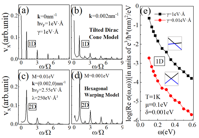
Figure 2: Intra-band high harmonic generation of (a, b) the 1D tilted Dirac cone model and (c, d) the 2D hexagonal warping model. The harmonics are generated from a Fourier transform of the velocity in the x direction, which changes abruptly at the $k_{x}=0$ point. (e) The real part of intra-band nonlinear optical conductivity obtained from Eq. (17). For the 1D tilted Dirac cone model Eq. (18), as the tiltness $\gamma$ increases, the nonlinear optical conductivity increases significantly.

In below we use density functional theory (DFT) and non-equilibrium Green’s function software to calculate the electronic properties of materials from chemical elements. The electrostatic potential energy calculation of Si pn-junction, the electronic properties calculation of $\rm{B_{8}}$, $\rm{AlN}$ and the orbital projection band calculation for $\rm{TaAs}$ and $\rm{LiNbO_{3}}$ are performed by using a first-principles method based on DFT [42], as implemented in the Nanodcal and DS-PAW which are programs under the Device Studio platform, for superconductor $\rm{NbN}$ we use Quantum ESPRESSO. The DS-PAW is based on the plane wave basis and the projector augmented wave (PAW) representation,the Nanodcal is a first principles computing software based on linear combined atomic orbital basis and non-equilibrium Green’s function-density functional theory[43]. The Perdew-Burke-Ernzerhof (PBE) exchange-correlation energy functional within the generalized gradient approximation (GGA) are employed [44, 45]. For $\rm{NbN}$, SG15-type [46] norm-conserving pseudo-potential is employed [47]. The electronic iteration convergence criterion is set to $10^{-4}$ $\rm{eV}$, for $\rm{NbN}$ it is $10^{-5}$ a.u (27.21146×$10^{-5}$ $\rm{eV}$). The wave functions were expanded in plane waves up to a kinetic energy cutoff of 500 $\rm{eV}$ for $\rm{B_{8}}$ and $\rm{AlN}$, 300 $\rm{eV}$ for $\rm{TaAs}$ and $\rm{LiNbO_{3}}$, 120 Ry (1632.6 eV) for $\rm{NbN}$ and 480 Ry (6530.4 eV) for the charge density cutoff of $\rm{NbN}$, 100 Hartree (2721.1 eV) for Si pn junction. The Brillourin zone integration is obtained by using a k-point sampling mesh of $10\times 13\times 1$ for $\rm{B_{8}}$, $14\times 14\times 14$ for $\rm{AlN}$, $12\times 12\times 4$ for $\rm{TaAs}$, $10\times 10\times 4$ for $\rm{LiNbO_{3}}$, $10\times 10\times 2$ for hexagonal NbN, $10\times 10\times 10$ for cubic NbN, $11\times 11\times 1$ for single layer Si pn junction, $6\times 11\times 1$ for bilayer Si pn junction, generated according to the Gamma-centered method. We have included the contribution of spin-orbit coupling (SOC) in our calculations of $\rm{TaAs}$ and $\rm{LiNbO_{3}}$. The thickness of the vacuum layer was set for 20 Å in calculations of $\rm{B_{8}}$, which can reduce the interactions between the adjacent layers. In the Si pn junction modeling, we use the virtual crystal approximation (VCA) method to realize p-type and n-type vacancy doping.

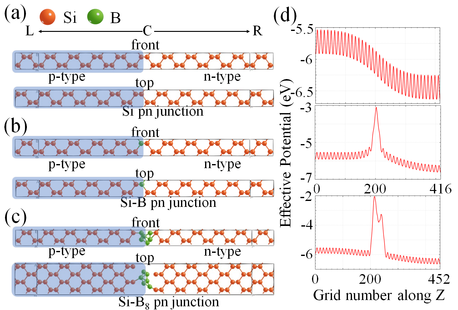
Figure 3: (a) The atomic structure of a Silicon pn-junction. The blue shaded region is the p-type Silicon. (b) The silicon pn-junction with a Boron atom replacing the Silicon atom in the middle of the junction. (c) A layer of $\rm{B_{8}}$ is inserted into the Silicon pn-junction. (d) The potential energy of the three devices (a), (b) and (c), from top to bottom respectively. The real space is divided into grids for simultaneous solving of the Poisson’s equation and the effective equation from DFT, using the Nanodcal software.

In Fig. 3 (a), we provide the top and front view of the Silicon pn junction, generated from the Device Studio platform. The device consists of 11 Silicon cells, the length of central region is 48.8754 Å (9 Silicon cells), the length of left or right electrode is 5.4306 Å (1 Silicon cell). In Fig. 3 (b), the Silicon pn junction is replaced by one Boron atom in the middle. In Fig. 3 (c), the Silicon pn-junction is expanded in the top view, to make it large enough for the insertion of $\rm{B_{8}}$ in the middle of the device. The length of the center region increases slightly to 53.20175 Å. We use the VCA of Nanodcal to achieve p-type and n-type doping. The doping concentration of p-type is 0.999, and for n-type it is 1.001. In Fig. 3 (d), the central region length of Si pn junction and Si-B pn junction is the same 48.8754 Å, and the calculated real space grid number is 416. In Si-$\rm{B_{8}}$ pn junction, due to the insertion of $\rm{B_{8}}$ cell, the central region length changes to 53.20175 Å, and the real space grid number is 452. Without applied external voltage on the 3 devices, the potential energy displays obvious asymmetry in the real space. Moreover, for Si-B pn-junction, there is an obvious peak at the location of B atom, and for Si-$\rm{B_{8}}$ pn-junction, there are two peaks at the position where $\rm{B_{8}}$ cell is inserted, a sharp main peak and a smaller side peak, asymmetric in the real space.

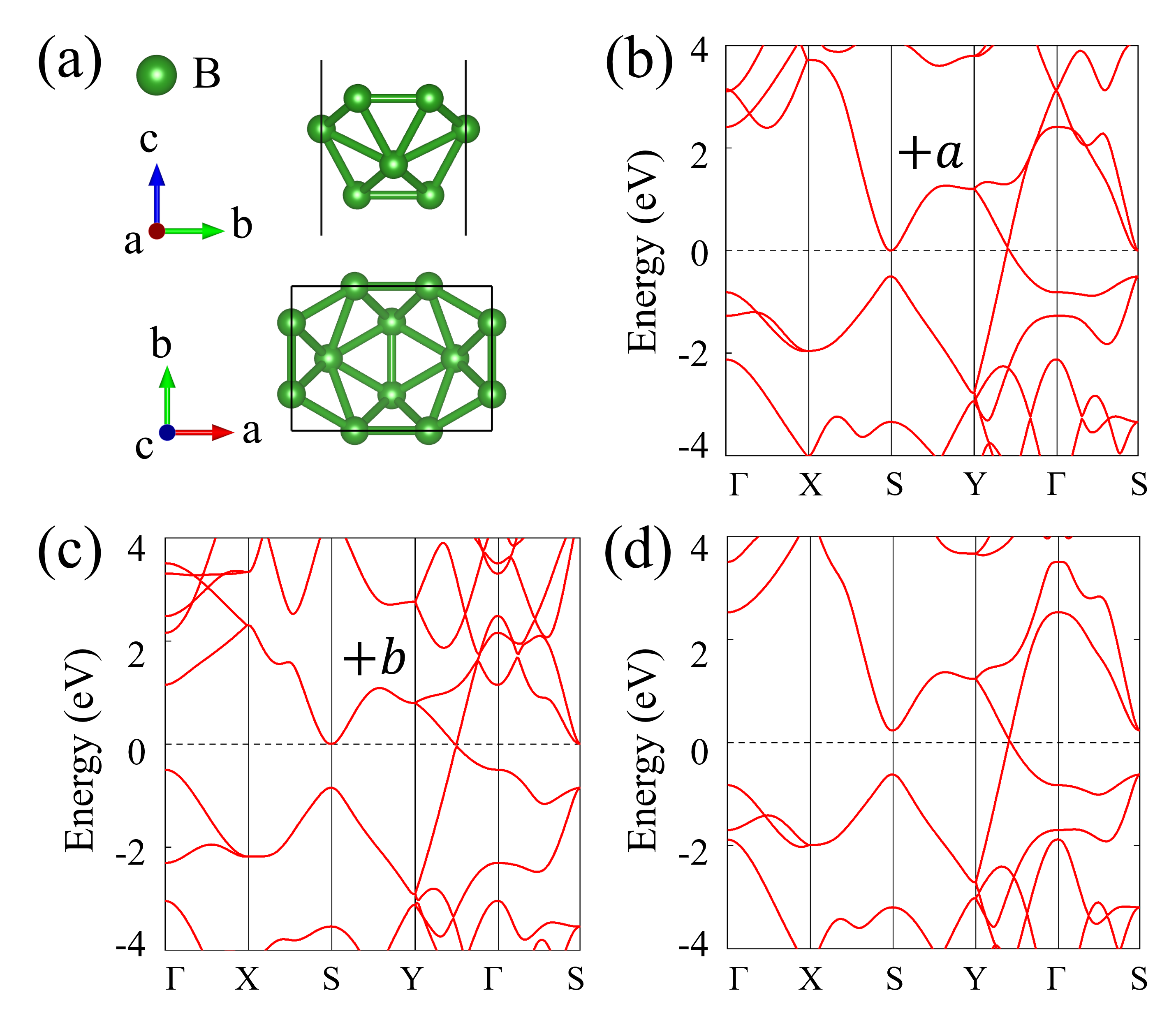
Figure 4: (a) The lattice structure of $\rm{B_{8}}$. (b) After stretching along the a axis, the tiltness of the Dirac cone changes slightly. (c) After stretching along the b axis. the tiltness of the Dirac cone changes significantly. The strength of the stretching is to change the original lattice constant by 10%. (d) The original band structure of $\rm{B_{8}}$.

In Fig. 4, we present the lattice and band structure of $\rm{B_{8}}$. The band gap near the high symmetry point $S$ changes significantly from 0.859 $\rm{eV}$ to 0.507 $\rm{eV}$. Stretching along the b-axis of $\rm{B_{8}}$, the bands near the high symmetry point $\Gamma$ shift upwards, resulting a tilt of the Dirac cone in the $\rm{Y}$-$\Gamma$ path. Stretching along the a-axis, the bands are not changed significantly.

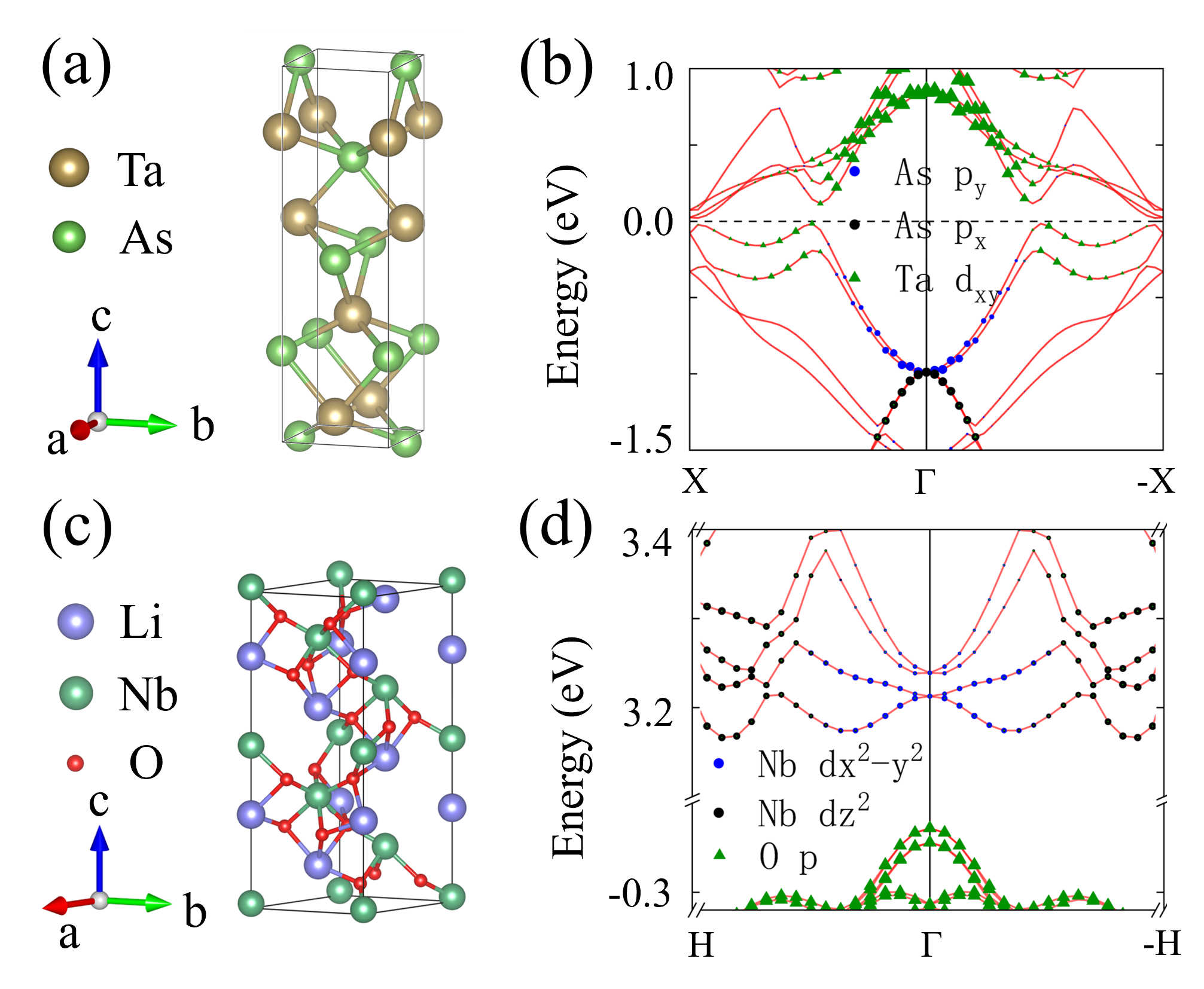
Figure 5: (a) The structure of $\rm{TaAs}$. (b) The projected band for $\rm{TaAs}$. The high-symmetric points are X(0.0, ${\frac{1}{2}}$, 0.0), $\rm{\Gamma}$(0.0, 0.0, 0.0), -X(0.0, -${\frac{1}{2}}$, 0.0). (c) The structure of $\rm{LiNbO_{3}}$. (d) The projected band for $\rm{LiNbO_{3}}$. The high-symmetric points are H(${\frac{1}{3}}$, ${\frac{1}{3}}$, ${\frac{1}{2}}$), -H(${-\frac{1}{3}}$, ${-\frac{1}{3}}$, ${-\frac{1}{2}}$).

In Fig. 5, we present the structures and the projected bands of $\rm{TaAs}$ and $\rm{LiNbO_{3}}$. Around the $\Gamma$ point, the contribution to the conduction band of $\rm{TaAs}$ mainly comes from the $d_{xy}$ orbital of $\rm{Ta}$ atom, while for $\rm{LiNbO_{3}}$, it mainly comes from the $d_{x^{2}-y^{2}}$ orbital of $\rm{Nb}$ atom, and switch to the $d_{z^{2}}$ orbital as the momentum moves away from the $\Gamma$ point. The contribution to the valence band of $\rm{TaAs}$ comes from both $p_{x}$ and $p_{y}$ orbitals of $\rm{As}$ atom, while for $\rm{LiNbO_{3}}$, it comes from the $p_{x}$, $p_{y}$, and $p_{z}$ orbitals of $\rm{O}$ atom. Moreover, $\rm{LiNbO_{3}}$ (also in other oxides [48]) has a wide band gap about 3.367 $\rm{eV}$ while $\rm{TaAs}$ is a gapless semimetal. Fig. 5 (d) shows only 80% of the length on the ${\Gamma}$-H path. Although both materials are noncentrosymmetric in the real space, we do not find any asymmetry of the band structure in the Brillouin zone. So the intra-band part of the second order nonlinear optical conductivity is zero.

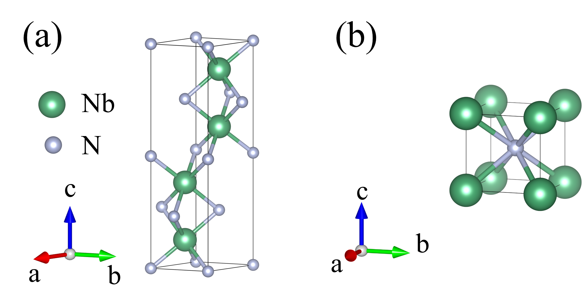
Figure 6: (a) Lattice structure of the hexagonal $\epsilon$-NbN ($\rm{P6_{3}}$/mmc, No. 194) with an estimate of $T_{c}$ = 10.230 K. (b) Lattice structure of the cubic NbN ($\rm{Pm\overline{3}m}$, No. 221) with an estimate of $T_{c}$ = 2.048 K.

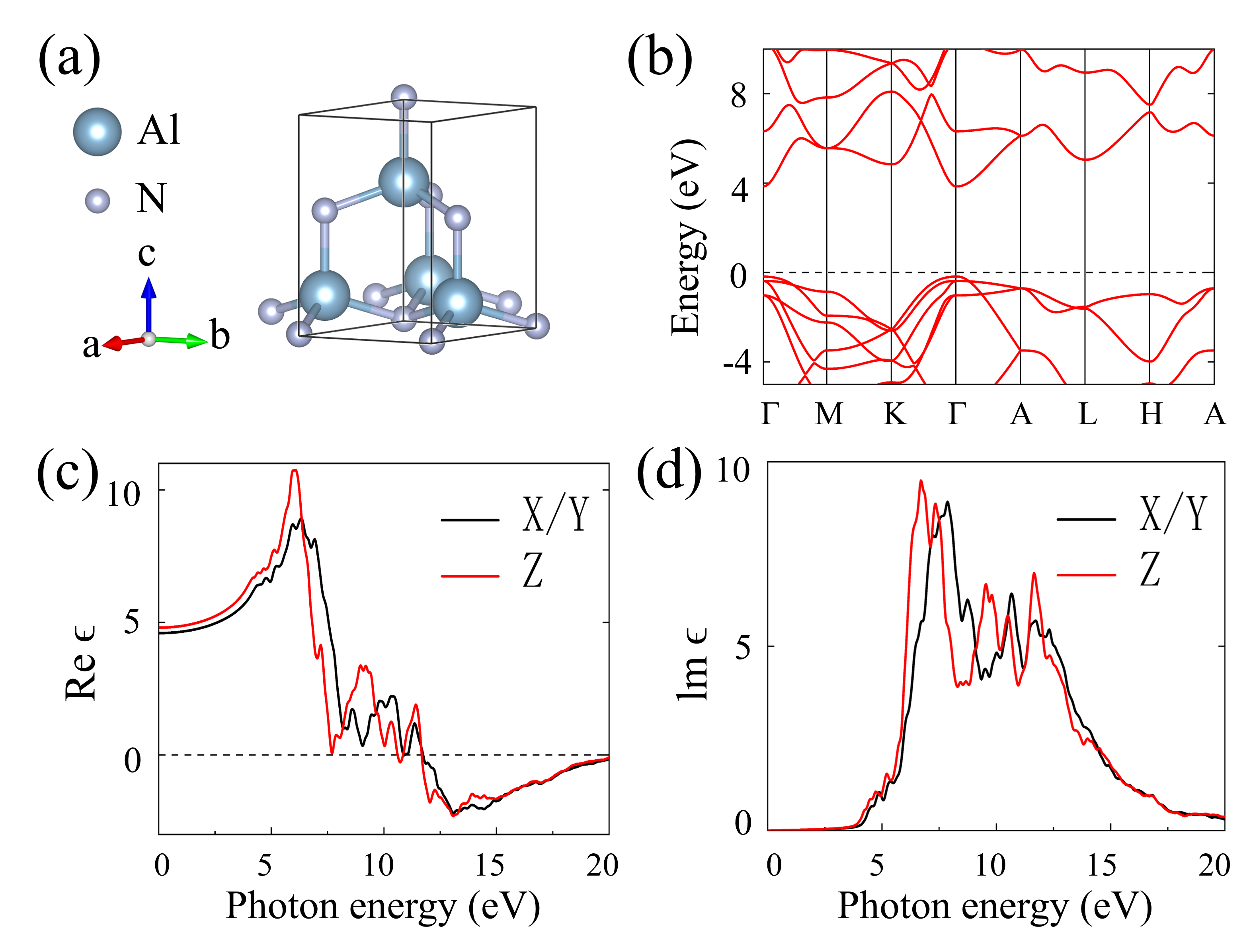
Figure 7: (a) The lattice structures of AlN, and the blue and grey atoms are Al and N. (b) The energy band of AlN. (c) The real part of the dielectric function of AlN along X,Y and Z direction. Slight anisotropy is observed. (d) The imaginary part of the dielectric function of AlN.

In a Josephson junction, the inter-layer supercurrent $J_{s}$ is determined from the phase difference $\phi$ of the two superconducting layers, $J_{s}=J_{c}\rm{sin}(\phi)$, quite different from the conventional current $J=\sigma E$. Electric and magnetic field in layered superconductors (Josephson junctions) form plane-wave-like Josephson plasma waves (JPW) or soliton-like Josephson vortices (JV), both are solutions of the sine-Gordon equations of $\phi$ [14]. The Josephson plasma frequency $\omega_{J}$ is in the Terahertz range. Because of $\rm{sin}(\phi)\approx\phi-\phi^{3}/6$, nonlinear JPW could propagate below, and very close to $\omega_{J}$. Coherent emission from JPW [49] or Cherenkov radiation from JV lattices are proposed. The current-current-current correlation is known as the third moment of shot noise of the Josephson junction, and changes the average thermal escape rate [50]. The Josephson plasma frequency $\omega_{J}=\sqrt{\frac{8\pi neDJ_{c}}{\hbar\epsilon}}$ [14], where $D$ is the total thickness of an insulating layer and a superconducting layer, $\epsilon$ is the dielectric constant of the insulating layers, $n=N/2$, $N$ is the electron number of a superconducting quasiparticle, for Cooper pair, $N=2$. $J_{c}$ is the critical current density of the junction structure.

In Fig. 6, we present the structure of (a) hexagonal $\varepsilon$-NbN and (b) the cubic NbN [51, 52]. The superconducting transition temperature ($T_{c}$) is determined by Allen-Dynes modified McMillan equation [53, 54, 55, 56], $k_{B}T_{c}=\frac{\hbar\omega_{\rm{log}}}{1.2}\mathrm{exp}\left[\frac{-1.04(1+\lambda)}{\lambda(1-0.62\mu^{*})-\mu^{*}}\right]$, with the parameters estimated from Quantum ESPRESSO. For hexagonal $\epsilon$-NbN the logarithmic average $\omega_{\rm{log}}$ = 350.492 K (30.244 meV), the electron-phonon coupling $\lambda$ = 0.65364 and the Coulomb repulsion $\mu^{*}$ = 0.10, for cubic-NbN, $\omega_{\rm{log}}$ = 623.388K (53.792 meV), $\lambda$ = 0.41705 and $\mu^{*}$ = 0.12. The pressure is at 0.1 MPa. It is found that $T_{c}$ = 10.230 K for hexagonal $\epsilon$-NbN and $T_{c}$ = 2.048 K for cubic-NbN. In Fig. 7, we present the structure, band and the dielectric function of insulating layer $\rm{AlN}$. The dielectric function along the x/y axis is different from that along the z axis. The real part of the dielectric function becomes negative in the high frequency region.

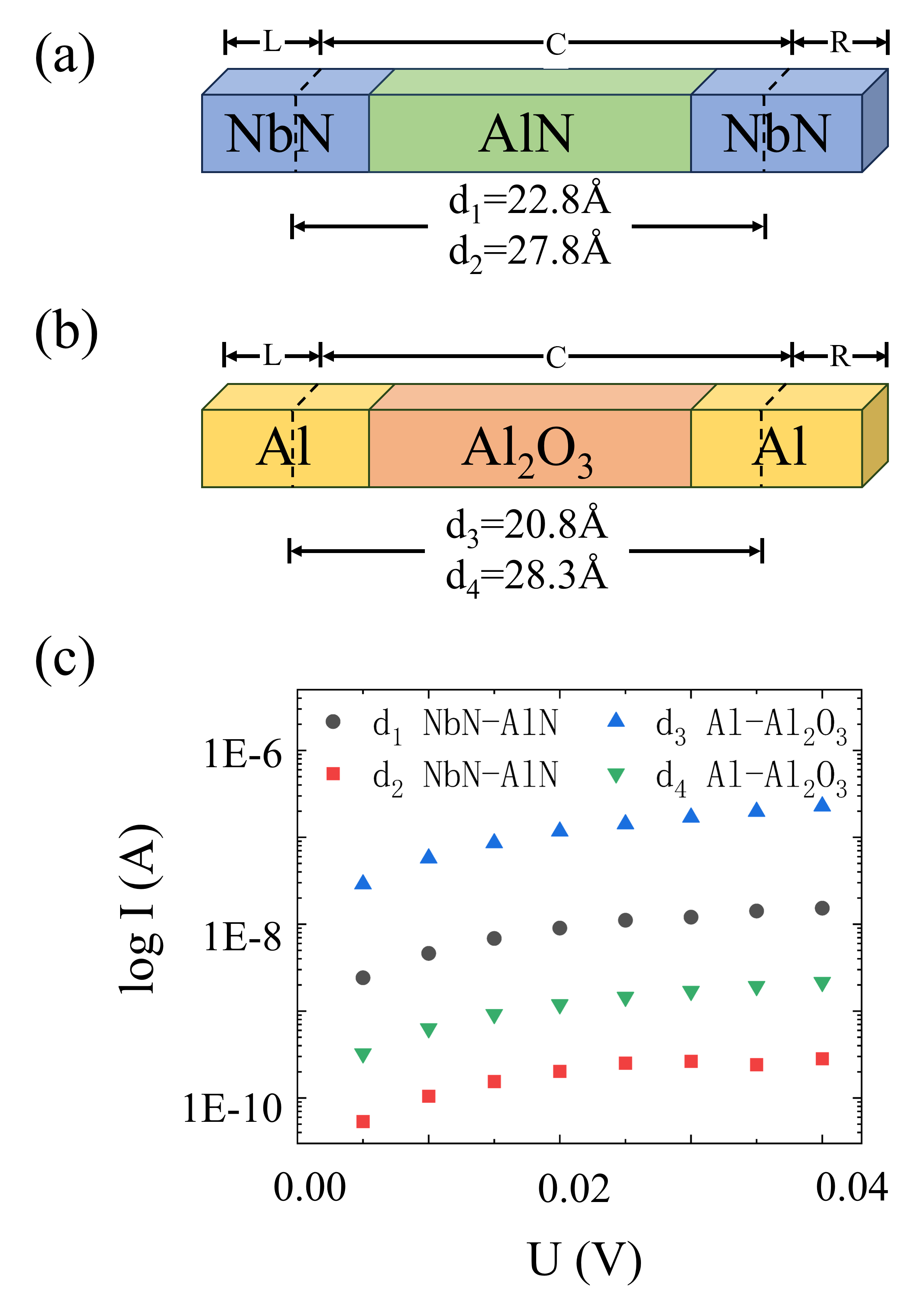
Figure 8: Schematic of (a) NbN-AlN-NbN and (b) Al-Al₂O₃-Al heterojunction. (c) The I-V curve of the four devices with different length of the central region. The resistance calculated from the I-V curve is important for optimizing the quality factor of the Josephson junction cavity. As the heat dissipated from the cavity is directly controlled by the resistance.

In Fig. 8, We provide schematic of the NbN-AlN-NbN and Al-Al₂O₃-Al hetero-junction devices. The details of the structure is provided in the supplementary material. The device is divided into three parts: the left electrode (L), the central scattering region (C), and the right electrode (R). In Fig. 8 (c), we observe that for similar thickness of the central scattering region, the resistance of NbN-AlN-NbN junction is significantly larger than that of the Al-Al₂O₃-Al junction, as one compares the black dots and the blue triangle. As the thickness increases, the resistance of both devices increases. For a given voltage, larger resistance means smaller dissipation of heat.

To conclude, we develop the velocity-operator approach to calculate the nonlinear optical conductivity from a current-current-current correlation. We establish connections between our approach and the position-operator approach. We investigate both the intra-band and inter-band contributions to the nonlinear optical conductivity, which are computable from a wannier Hamiltonian fitted from DFT. The intra-band is not emphasized in the visible and ultraviolet frequency band, but has a strong sum-frequency generation in the THz frequency band, predicted by a titled Dirac cone model. The abrupt change of velocity and the asymmetry in the momentum space are the key requirement for such an intra-band process. Similar mechanism is used in the step recovery diode to do a up-conversion of frequency from GHz to THz. Nonlinear Josephson plasmon devices also oscillate in the THz frequency region. The superconductor transition temperature and the dielectric function of the insulator are analyzed for these devices. The resistance of the NbN-AlN-NbN and Al-Al₂O₃-Al hetero-junction devices are calculated.

- [1] A. Nahata, A.S. Weling and T.F. Heinz, A wideband coherent terahertz spectroscopy system using optical rectification and electro-optic sampling, Appl. Phys. Lett. 69, 2321-2323 (1996).
- [2] Q. Wu and X. C. Zhang, Free-space electro-optic sampling of mid-infrared pulses, Appl. Phys. Lett. 71, 1285-1286 (1997).
- [3] János Hebling, Gábor Almási, Ida Z. Kozma, and Jürgen Kuhl, Velocity matching by pulse front tilting for large-area THz-pulse generation, Optics Express 10 (21), 1161-1166 (2002).
- [4] S. M. Young and A. M. Rappe, First Principles Calculation of the Shift Current Photovoltaic Effect in Ferroelectrics, Phys. Rev. Lett. 109, 116601 (2012).
- [5] S. M. Young, F. Zheng and A. M. Rappe, First-Principles Calculation of the Bulk Photovoltaic Effect in Bismuth Ferrite, Phys. Rev. Lett. 109, 236601 (2012).
- [6] I. Grinberg, D. V. West, M. Torres, G. Gou, D. M. Stein, L. Wu, G. Chen, E. M. Gallo, A. R. Akbashev, P. K. Davies, J. E. Spanier, A. M. Rappe, Perovskite oxides for visible light-absorbing ferroelectric and photovoltaic materials, Nature 503, 509–512 (2013).
- [7] W. Nie, H. Tsai, R. Asadpour, J.-C. Blancon, A. J. Neukirch, G. Gupta, J. J. Crochet, M. Chhowalla, S. Tretiak, M. A. Alam, H.-L. Wang, A. D. Mohite, High-efficiency solution processed perovskite solar cells with millimeter-scale grains, Science 347, 522–525 (2015).
- [8] D. Shi, V. Adinolfi, R. Comin, M. Yuan, E. Alarousu, A. Buin, Y. Chen, S. Hoogland, A. Rothenberger, K. Katsiev, Y. Losovyj, X. Zhang, P. A. Dowben, O. F. Mohammed, E. H. Sargent, O. M. Bakr, Low trap-state density and long carrier diffusion in organolead trihalide perovskite single crystals, Science 347, 519–522 (2015).
- [9] D. W. de Quilettes, S. M. Vorpahl, S. D. Stranks, H. Nagaoka, G. E. Eperon, M. E. Ziffer, H. J. Snaith, D. S. Ginger, Impact of microstructure on local carrier lifetime in perovskite solar cells, Science 348, 683–686 (2015).
- [10] L. Z. Tan and A. M. Rappe, Enhancement of the Bulk Photovoltaic Effect in Topological Insulators, Phys. Rev. Lett. 116, 237402 (2016).
- [11] A. M. Cook, B. M. Fregoso, F. de Juan, S. Coh and J. E. Moore, Design principles for shift current photovoltaics, Nature Communications 8, 14176 (2017).
- [12] P. A. Franken, A. E. Hill, C. W. Peters, and G. Weinreich, Generation of Optical Harmonics, Phys. Rev. Lett. 7, 118 (1961).
- [13] H. W. K. Tom, T. F. Heinz, and Y. R. Shen, Second-Harmonic Reflection from Silicon Surfaces and Its Relation to Structural Symmetry, Phys. Rev. Lett. 51, 1983 (1983).
- [14] S. Savel’ev, A. L. Rakhmanov, V. A. Yampol’skii, F. Nori, Analogues of nonlinear optics using terahertz Josephson plasma waves in layered superconductors, Nature Physics 2, 521-525 (2006)
- [15] A. F. Kockum, A. Miranowicz, V. Macrí, S. Savasta, F. Nori, Deterministic quantum nonlinear optics with single atoms and virtual photons, Phys. Rev. A 95, 063849 (2017).
- [16] A. F. Kockum, V. Macrí, L. Garziano, S. Savasta, F. Nori, Frequency conversion in ultrastrong cavity QED, Scientific Reports 7, 5313 (2017).
- [17] R. Stassi, V. Macrí, A. F. Kockum, O.D. Stefano, A. Miranowicz, S. Savasta, F. Nori, Quantum Nonlinear Optics without Photons, Phys. Rev. A 96, 023818 (2017).
- [18] X. Gu, A. F. Kockum, A. Miranowicz, Y.X. Liu, F. Nori, Microwave photonics with superconducting quantum circuits Physics Reports 718-719, pp. 1-102 (2017).
- [19] J. E. Sipe and E. Ghahramani, Nonlinear optical response of semiconductors in the independent-particle approximation, Phys. Rev. B 48, 11705 (1993).
- [20] S. A. Mikhailov, Theory of the giant plasmon-enhanced second-harmonic generation in graphene and semiconductor two-dimensional electron systems, Phys. Rev. B. 84, 045432 (2011).
- [21] Daria Smirnova and Yuri S. Kivshar, Second-harmonic generation in subwavelength graphene waveguides, Phys. Rev. B. 90, 165433 (2014).
- [22] N. Bloembergen, Nonlinear optics (W. A. Benjamin Inc., New York, 1965).
- [23] See Supplemental Material at [URL] for the discussion of the general formula of the nonlinear conductivity tensor, the expansion of the imaginary frequency Green’s function into a sum of the real frequency spectral function, the calculation of the sum in imaginary frequency, and the evaluation of the trace of the matrix elements.
- [24] Zhou Li and F. Nori, Nonlinear response in a noncentrosymmetric topological insulator, Phys. Rev. B 99, 155146 (2019).
- [25] X. Jiang, L. Kang, J. Wang, B. Huang, Giant Bulk Electrophotovoltaic Effect in Heteronodal-Line Systems, Phys. Rev. Lett. 130 (25), 256902 (2023).
- [26] X. Huang, X. Jiang, B. Huang,and Z. Li, Nonlocal optical conductivity of Fermi surface nesting materials, Sci. China Phys. Mech. 63, 1 (2022).
- [27] L. Fu, Hexagonal Warping Effects in the Surface States of the Topological Insulator , Phys. Rev. Lett 103, 266801 (2009).
- [28] Zhou Li and J. P. Carbotte, Hexagonal warping on spin texture, Hall conductivity, and circular dichroism of topological insulators, Phys. Rev. B 89, 165420 (2014).
- [29] Zhou Li and J. P. Carbotte, Hexagonal warping on optical conductivity of surface states in topological insulator , Phys. Rev. B 87, 155416 (2013).
- [30] S. Y. Xu et al., Topological Phase Transition and Texture Inversion in a Tunable Topological Insulator, Science 332, 560 (2011).
- [31] S. Y. Xu et al., Hedgehog spin texture and Berry’s phase tuning in a magnetic topological insulator, Nature Phys. 8,616 (2012).
- [32] Y. L. Chen et.al, Massive Dirac Fermion on the Surface of a Magnetically Doped Topological Insulator, Science 329, 659 (2010).
- [33] M. Z. Hasan and C. L. Kane, Colloquium: Topological insulators, Rev. Mod. Phys. 82, 3045 (2010).
- [34] X.-L. Qi and S.-C. Zhang, Topological insulators and superconductors, Rev. Mod. Phys. 83, 1057 (2011).
- [35] J. E. Moore, The birth of topological insulators, Nature 464, 194 (2010).
- [36] D. Hsieh et al., Observation of Unconventional Quantum Spin Textures in Topological Insulators, Science 323, 919 (2009).
- [37] Y. L. Chen et al., Experimental Realization of a Three-Dimensional Topological Insulator, , Science 325, 178 (2009).
- [38] D. Hsieh et al., A tunable topological insulator in the spin helical Dirac transport regime, Nature(London) 460, 1101 (2009).
- [39] K. N Okada, Y. Takahashi, M. Mogi, R. Yoshimi, A. Tsukazaki, K. S. Takahashi, N. Ogawa, M. Kawasaki and Y. Tokura, Observation of topological Faraday and Kerr rotations in quantum anomalous Hall state by terahertz magneto-optics. Nat. Commun. 7, 12245 (2016).
- [40] K. Yasuda, A. Tsukazaki, R. Yoshimi, K. S. Takahashi, M. Kawasaki, and Y. Tokura, Large Unidirectional Magnetoresistance in a Magnetic Topological Insulator. Phys. Rev. Lett. 117, 127202 (2016).
- [41] Zi-Yuan Li, Qi Li and Zhou Li, High-order harmonic generations in tilted Weyl semimetals, Chinese Phys. B 31 124204 (2022).
- [42] G. Kresse, D. Joubert, From ultrasoft pseudopotentials to the projector augmented wave method Phys. Rev. B 59, 1758-1775 (1999).
- [43] P. E. Blochl, Phys. Rev. B 50, 17953-17979 (1994).
- [44] J. P. Perdew, K. Burke, M. Ernzerhof, Generalized Gradient Approximation Made Simple, Phys. Rev. Lett. 77, 3865-3868 (1996).
- [45] S. Grimme, Semiempirical GGA-type density functional constructed with a long-range dispersion correction, J. Comput. Chem. 27, 1787-1799 (2006).
- [46] K. Lejaeghere, G. Bihlmayer, T. Björkman, et al, Reproducibility in density functional theory calculations of solids, Science, 351(6280) (2016).
- [47] D. R. Hamann, Optimized norm-conserving Vanderbilt pseudopotentials, Physical Review B, 88(8), 085117 (2013).
- [48] B. H. Lei, S. Pan, Z. Yang, C. Cao, D. J. Singh, Second harmonic generation susceptibilities from symmetry adapted Wannier functions, Phys. Rev. Lett. 125, 187402 (2020).
- [49] D. Nicoletti, M. Buzzi, M. Fechner, P. E. Dolgirev, M. H. Michael, J. B. Curtis, E. Demler, G. D. Gu, and A. Cavalleri, Coherent emission from surface Josephson plasmons in striped cuprates, PNAS 119, 39, e2211670119 (2022).
- [50] A. V. Timofeev, M. Meschke, J. T.Peltonen, T. T. Heikkila and J. P. Pekola, Wideband Detection of the Third Moment of Shot Noise by a Hysteretic Josephson Junction, Phys. Rev. Lett. 98, 207001 (2007).
- [51] S. Kim, H. Terai, T. Yamashita, et al. Enhanced coherence of all-nitride superconducting qubits epitaxially grown on silicon substrate, Communications Materials 2, 98 (2021).
- [52] R. Espiau de Lamaëstre, P. Odier, J. C. Villégier, Microstructure of NbN epitaxial ultrathin films grown on A-, M-, and R-plane sapphire, Appl. Phys. Lett. 91, 232501 (2007).
- [53] G. M. Eliashberg, Interactions between electrons and lattice vibrations in a superconductor, Sov. Phys. JETP 11 (3), 696-702 (1960).
- [54] P. B. Allen, Neutron spectroscopy of superconductors, Phys. Rev. B 6(7), 2577 (1972).
- [55] Yansun Yao, J. S. Tse, K. Tanaka, F. Marsiglio, and Y. Ma, Superconductivity in lithium under high pressure investigated with density functional and Eliashberg theory, Phys. Rev. B 79, 054524 (2009).
- [56] F. Giustino, Electron-phonon interactions from first principles, Rev. Mod. Phys. 89(1), 015003 (2017).