LCEN: A Novel Feature Selection Algorithm for Nonlinear, Interpretable Machine Learning Models

Abstract

Interpretable architectures can have advantages over black-box architectures, and interpretability is essential for the application of machine learning in critical settings, such as aviation or medicine. However, the simplest, most commonly used interpretable architectures (such as LASSO or EN) are limited to linear predictions and have poor feature selection capabilities. In this work, we introduce the LASSO-Clip-EN (LCEN) algorithm for the creation of nonlinear, interpretable machine learning models. LCEN is tested on a wide variety of artificial and empirical datasets, creating more accurate, sparser models than other commonly used architectures. These experiments reveal that LCEN is robust against many issues typically present in datasets and modeling, including noise, multicollinearity, data scarcity, and hyperparameter variance. LCEN is also able to rediscover multiple physical laws from empirical data and, for processes with no known physical laws, LCEN achieves better results than many other dense and sparse methods – including using 10.8 times fewer features than dense methods and 8.1 times fewer features than EN on one dataset, and is comparable to an ANN on another dataset.

1 Introduction

Statistical models are powerful tools to explain, predict, or describe natural phenomena (Shmueli, 2010). They connect independent variables (also called “inputs” or “features”) to dependent variables (also called “outputs” or “labels”) to test causal hypotheses, predict novel outputs from known inputs, or summarizing the data structure (Shmueli, 2010). Many model architectures exist, including linear, ensemble-based, and deep learning models. Complex architectures are claimed to have greater capability to model phenomena due to their lower bias, but their intricate and numerous mathematical transformations prevent humans from understanding how an output was predicted by a model, or the relative or absolute importance of the inputs. Moreover, a lack of transparency may prevent the model from being trusted in critical or sensitive applications (Hong et al., 2020).

As summarized by Ribeiro et al. (2016), there are two main methods to increase interpretability: the use of model-agnostic algorithms, which extract interpretable explanations a posteriori and work for any architecture, or the direct use of interpretable architectures. Interpretable architectures include “decision trees, rules, additive models, attention-based networks, and sparse linear models” (Ribeiro et al., 2016). As elaborated in the review of Rudin (2019), interpretable architectures can have many advantages over black-box or a posteriori explanations, including the ability to assist researchers in refining the model and data, or better highlighting scenarios in which the model fails or lacks robustness. Special attention should be given to sparse models, which identify the most important features, can make the model more robust to variations in the input data, and significantly improve the model’s interpretability (Rudin, 2019). At the same time, even a linear model or decision tree/rules can become unwieldy and uninterpretable if hundreds or thousands of coefficients or rules are present.

Feature selection is the process of selecting the most important features in a model to increase its robustness or interpretability. Many criteria for feature selection exist (Heinze et al., 2018), including significance based on p-values (using a univariate, iterative/stepwise, or global method), using information criteria (such as the AIC (Akaike, 1974) and BIC (Schwarz, 1978)), using penalties (such as in LASSO (Santosa & Symes, 1986) and elastic net [EN] (Zou & Hastie, 2005)), criteria based on changes in estimates, and expert knowledge. While no method is superior for all problems, different works have evaluated and criticized these criteria. For example, stepwise regression is one of the most commonly used methods in many fields thanks to its computational simplicity and ease of understanding (Whittingham et al., 2006; Heinze et al., 2018; Smith, 2018). However, stepwise regression is prone to ignoring features with causal effects, including irrelevant features, generating excessively small confidence intervals, and producing incorrect/biased parameters (Whittingham et al., 2006; Smith, 2018). LASSO is simple and computationally cheap, and has performed well for some problems (Hebiri & Lederer, 2013; Tian et al., 2015; Pavlou et al., 2016), but can overselect irrelevant variables, can select only as many features as there are samples, and does not handle multicollinear data well (Heinze et al., 2018; Zou & Hastie, 2005).

Most feature selection methods apply only in linear contexts (or have been applied primarily in linear contexts). For example, the only sparse models referenced in the highly cited review by Ribeiro et al. (2016) are linear. The main sparse architectures (LASSO, EN, and their variants) are linear regressors. Later works consider sparse nonlinear models, to address the fact that many natural and industrial processes are nonlinear. McConaghy (2011), Brewick et al. (2017), and Sun & Braatz (2020) defined sets of features consisting of polynomials (all works), interactions (all works), and/or non-polynomials (McConaghy, 2011; Sun & Braatz, 2020). ALVEN, the model architecture from Sun & Braatz (2020), uses an f-test for each feature (including the expanded set of features) to determine whether to keep a feature in the final EN model. However, this f-test has very poor feature selectivity, as nearly all features are selected when traditional values of $\alpha$ ($0.001\leq\alpha\leq 0.05$) are used. Furthermore, the ordering of the features with respect to their p-values does not follow their relevance, as many irrelevant features are among those with the lowest p-values, and relevant features can be among those with the highest p-values (including p $\gg 0.05$).

To create nonlinear, interpretable machine learning models with high predictive and descriptive power, we propose the LASSO-Clip-EN (LCEN) algorithm. This algorithm generates an expanded set of features (such as in ALVEN) and performs feature selection and model fitting. The algorithm is tested on artificial and empirical data, successfully rediscovering physical laws from data belonging to multiple different areas of knowledge with errors < 2% on the coefficients, a value within the empirical noise of the datasets. On datasets from processes whose underlying physical laws are not yet known, LCEN attains lower RMSEs than sparse and dense methods and simultaneously leads to sparser models than alternative architectures.

2 Methods

2.1 Datasets

Multiple datasets are used to test the performance of the LCEN algorithm (summarized in Table A1). These datasets can be divided into three categories: artificial data [“Linear, 5-variable polynomial”, “Multicollinear data”, “Relativistic energy”, and “4th-degree, univariate polynomial”], empirical data from processes with known physical laws [“CARMENES star data”, “Kepler’s 3rd Law”, and “Newton’s Law of Cooling”], and empirical data from processes with no known physical laws [“Diesel Freezing Point”, “Abalone”, and “Concrete Compressive Strength”]. The artificial data generated by us are used for an initial assessment of the LCEN algorithm and to investigate how properties of the data, such as noise or data range, affect its feature selection capabilities. Empirical data from processes with known physical laws are used to verify whether the LCEN algorithm can rediscover known physical laws using data with real properties. Empirical data from processes with no known physical laws are used to compare the performance of the LCEN algorithm against other linear and nonlinear models, including deep learning models. Further description of these datasets and how the artificial datasets are generated is available in Section A1.

All models tested in this work, with the exception of the model for the “Newton’s Law of Cooling” dataset, had their hyperparameters selected by 5-fold cross-validation. The separation between training and testing sets varied depending on the dataset. None of the artificial datasets or datasets containing empirical data from processes with known physical laws have a separate test set, as they are used to investigate the capability of the LCEN algorithm to select correct features (which occurs based on the training set). For the “Diesel freezing point” dataset, 30% of the dataset was randomly separated to form the test set. For the “Abalone” dataset, the last 1,044 entries (25%) were used as the test set as per Waugh (1995) and Clark et al. (1996). For the “Concrete Compressive Strength” dataset, 25% of the dataset was randomly separated to form the test set as per Yeh (1998).

2.2 Algorithm

The LCEN algorithm has five hyperparameters: alpha, which determines the regularization strength (as in the LASSO, EN, and similar algorithms); l1_ratio, which determines how much of the regularization of the EN step depends on the 1-norm as opposed to the 2-norm (as in the EN algorithm); degree, which determines the maximum degree for the basis expansion of the data (Table A2); lag, which determines the maximum number of previous time steps from which features are included (relevant only for dynamic models); and cutoff, which determines the minimum value a scaled parameter needs to have to not be eliminated during the clip step.

The LCEN algorithm (Algorithm 1) begins with the LASSO step, setting the l1_ratio to 1. Cross-validation on the training set is employed among all combinations of alpha, degree, and lag values. The values of degree and lag corresponding to the model with the lowest validation MSE are recorded, and parameters are obtained for this LASSO model. The next step in the LCEN algorithm is the clip step, in which parameters smaller than the cutoff are set to 0. Finally, the EN step involves cross-validation on the training set among all combinations of alpha and l1_ratio, using the values of degree and lag obtained in the LASSO step. A final, nonlinear, and interpretable model, whose coefficients are subjected to the clip step again, is returned.

Algorithm 1 LASSO-Clip-EN (LCEN)

  Input: data $X$ and $y$; lists of hyperparameters alpha, l1_ratio, degree, lag; hyperparameter cutoff # LASSO step

  Temporarily set l1_ratio$=1$.

  for each combination in (alpha, degree, lag) do

     Perform cross-validation.

  end for

  Obtain the best hyperparameters from the above cross-validation.

  Obtain parameters with these hyperparameters.

  Record the best degree and lag hyperparameters. # Clip step

  Remove all parameters < cutoff. # EN step

  Restore l1_ratio to its original list of values.

  for each combination in (alpha, l1_ratio) do

     Perform cross-validation.

  end for

  Obtain the best hyperparameters from the above cross-validation.

  Obtain parameters with these hyperparameters. # Clip step II

  Remove all parameters < cutoff.

  return

3 Results

3.1 Artificial data highlight LCEN’s robustness to noise, multicollinearity, and hyperparameter variance

The first dataset used to validate the LCEN algorithm is a simple linear polynomial with five independent variables (“Linear, 5-variable polynomial”). This polynomial is of the form $y=-2.8X_{0}-2.7X_{1}-5.3X_{2}+4.3X_{3}+9.0X_{4}+\epsilon$. Datasets were created with increasing noise levels to determine how LCEN performs. For noise levels up to 119%, LCEN returned the correct polynomial among nonlinear and non-polynomial features with degree $\leq 3$ (Table 1). A noise level of 238%, the next level tested, led to the selection of one additional variable (${1}/{X_{4}}$), but the linear features had coefficients close to the ground truth. Furthermore, some of the coefficients did not display any appreciable change despite the increasing noise. This analysis highlights how LCEN is robust to noise in a scenario where all features are independent, even if the hyperparameters allow for extraneous features to potentially be selected by the algorithm.

Table 1: Coefficient values and MSEs to the ground truth for the “Linear, 5-variable polynomial” dataset at different noise levels. The coefficients are ordered such that the $n$th value corresponds to the coefficient of $X_{n}$.

Noise Coefficients MSE 0% -2.80, -2.70, -5.30, 4.30, 9.00 9.6$\times 10^{-14}$ 59.6% -2.82, -2.70, -5.27, 4.30, 9.01 2.2$\times 10^{-4}$ 119% -2.83, -2.70, -5.24, 4.30, 9.01 8.7$\times 10^{-4}$ 238% -2.85, -2.71, -5.20, 4.30, 8.73 1.7$\times 10^{-2}$

The first step of the LCEN algorithm uses LASSO, which has been claimed to underperform with multicollinear data (Heinze et al., 2018; Zou & Hastie, 2005). Therefore, tests using multicollinear data are done next. The goal is to verify whether LCEN can successfully determine the presence of two different but correlated variables, as LASSO prefers to select only one variable in this scenario (Zou & Hastie, 2005). Noise $\epsilon_{1}$, at different levels, was added to the $X_{0}$ variable to create a correlated variable $X_{1}$. A second noise $\epsilon_{2}$, also at different levels, was added to the final $y$ data. When $\epsilon_{1}=0$, both variables are equal and separation is not possible. However, at other $\epsilon_{1}$ values, the LCEN algorithm is very successful at identifying that two relevant variables exist and assigning correct coefficients to them (Figure 1). Specifically, when the noise level $\epsilon_{1}$ associated with the $X$ data (which indicates how different the $X$ variables are, as highlighted by the variance inflation factors [VIFs] in Fig. 1) is greater than the noise level $\epsilon_{2}$ associated with the $y$ data, LCEN can separate both variables with coefficient errors $\leq 5\%$. When both noise levels are similar, LCEN can separate both variables with coefficient errors between 5% and 10%. The $X$ data used in this experiment has very high multicollinearity (as shown by the VIFs); real data will typically have lower VIFs and thus be easier to separate using LCEN.

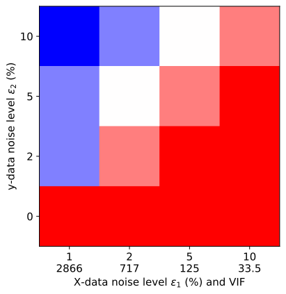
Figure 1: Output of the LCEN model at different $X$-data noise levels $\epsilon_{1}$ and $y$-data noise levels $\epsilon_{2}$. Bright red squares indicate both variables were selected and their coefficients had errors $\leq 5\%$. Light red squares indicate that both variables were selected and their coefficients had $5\%<\text{errors}\leq 10\%$. Squares in white indicate that both variables were selected and their coefficients had $10\%<\text{errors}\leq 20\%$. Light blue squares indicate that both variables were selected and their coefficients had errors > 20%. Bright blue squares indicate that only one of the variables was selected.

Next, a more complex equation is used to further validate LCEN. The “Relativistic energy” data contain mass and velocity values used to calculate $E^{2}=c^{4}m^{2}+c^{2}m^{2}v^{2}$. As before, datasets with increasing noise levels are created. The degree hyperparameter is allowed to vary between 1 and 6 in this experiment. LCEN selected only relevant features for a noise level $\leq 15\%$, and the coefficients were equal to the ground truth (Table 2). For a noise level of 20%, LCEN selected the two correct features, yet it also selected nonzero coefficients for $m$ and $m^{3}$. This error led to our hypothesizing that it is challenging to distinguish among $m$, $m^{2}$, and $m^{3}$ due to the low range of the data. Thus, another dataset with the same properties but a larger range of values for $m$ is created. LCEN performed better on this dataset, selecting only relevant features for all noise levels $\leq 30\%$ (the highest value tested) and having much lower errors in the estimated coefficients (Table 2). These experiments further highlight the robustness of LCEN and show how the range of the data can affect predictions.

Table 2: Coefficient values and corresponding relative RMSE to the ground truth for the “Relativistic energy” dataset at different noise levels. The first coefficient is for $m^{2}$ and should be $c^{4}=8.078$$\times$$10^{33}$ m⁴/s⁴; the second coefficient is for $m^{2}v^{2}$ and should be $c^{2}=8.988$$\times$$10^{16}$ m²/s². The first table is for the dataset with $1\leq m<10$, and the second table is for the dataset with $1\leq m<100$.

Noise Coefficients RMSE (%) 0% 8.077$\times 10^{33}$, 8.987$\times 10^{16}$ 0.013, 0.009 5% 8.081$\times 10^{33}$, 8.969$\times 10^{16}$ 0.043, 0.206 10% 8.085$\times 10^{33}$, 8.951$\times 10^{16}$ 0.097, 0.410 15% 8.089$\times 10^{33}$, 8.935$\times 10^{16}$ 0.139, 0.580 20% 5.579$\times 10^{33}$, 8.921$\times 10^{16}$ 30.94, 0.740

Noise Coefficients RMSE (%) 0% 8.078$\times 10^{33}$, 8.988$\times 10^{16}$ 0.002, 0.008 5% 8.077$\times 10^{33}$, 8.987$\times 10^{16}$ 0.014, 0.011 10% 8.077$\times 10^{33}$, 8.985$\times 10^{16}$ 0.055, 0.024 15% 8.068$\times 10^{33}$, 8.983$\times 10^{16}$ 0.116, 0.050 20% 8.070$\times 10^{33}$, 8.981$\times 10^{16}$ 0.093, 0.068 30% 8.061$\times 10^{33}$, 8.979$\times 10^{16}$ 0.210, 0.099

Finally, LCEN is compared with the feature selection algorithm in ALVEN (Sun & Braatz, 2020), which uses the same basis function expansion, but uses f-tests for feature selection. The “4th-degree, univariate polynomial” dataset is created as per Sun & Braatz (2021), such that $y=X+0.5X^{2}+0.1X^{3}+0.05X^{4}+\epsilon$, 30 $X$ points are available for training, and 1,000 $X$ points are available for testing. These conditions simulate the scarcity of data potentially present in real datasets while ensuring test errors can be predicted with high confidence. Sun & Braatz (2021) created four types of ALVEN models for this prediction: one that always uses degree = 4 (“unbiased model”), one that always uses degree = 2 (“biased model”), one that selects a degree between 1 and 10 based on cross-validation (“cv”), and one that selects a degree equal to 2 or 4 based on cross-validation (“cv limited order”). Sun & Braatz (2021) noted that the degree 4 “unbiased model” was the best at low noise levels, but its error quickly increases, leading to the degree 2 “biased model” becoming the best for noise levels > 75 (Figure 3 of Sun & Braatz (2021); reproduced with permission here as the left subfigure of Figure 2). The model with degree equal to 2 or 4 “cv limited order” was typically very close in performance to the best model at all noise levels, whereas the model with a degree between 1 and 10 “cv” had lower performance. Sun & Braatz (2021) explains these observations by the bias-variance tradeoff: at low noise levels, it is preferable to have the model follow the ground truth as closely as possible; thus, the degree 4 “unbiased model” was the best. However, once the noise level is sufficiently high, it becomes impossible to obtain enough signal within the data to compensate for the additional degrees of freedom (variance) in a 4th degree model; thus, the degree 2 “biased model” becomes the best. The degree between 1 and 10 “cv” model had lower performance due to its greater hyperparameter variance, and the degree equal to 2 or 4 “cv limited order” model struck a balance between the “unbiased model” and the “biased model”.

On this same dataset and using the same four types of models, LCEN attained median errors that are typically over 60% smaller than for ALVEN (Figure 2). Similarly to the models generated using ALVEN, the model with a degree between 1 and 10 “cv” had the lowest performance and the model with degree equal to 2 or 4 “cv limited order” had a performance between the degree 4 “unbiased model” and the degree 2 “biased model”. However, the degree 4 “unbiased model” was always the best model, no matter the noise level used. We attribute this considerable reduction in median test MSEs and the superiority of the degree 4 “unbiased model” created by LCEN to the improved feature selection algorithm, which is able to better resist variance due to noise and a large number of hyperparameters. This is corroborated by how the model with a degree between 1 and 10 “cv” tended to select degree = 4 at lower noise levels and degree = 2 at higher noise levels (Figure A1), showing how LCEN can automatically follow the hypothesis set by Sun & Braatz (2021) regarding the bias-variance tradeoff.

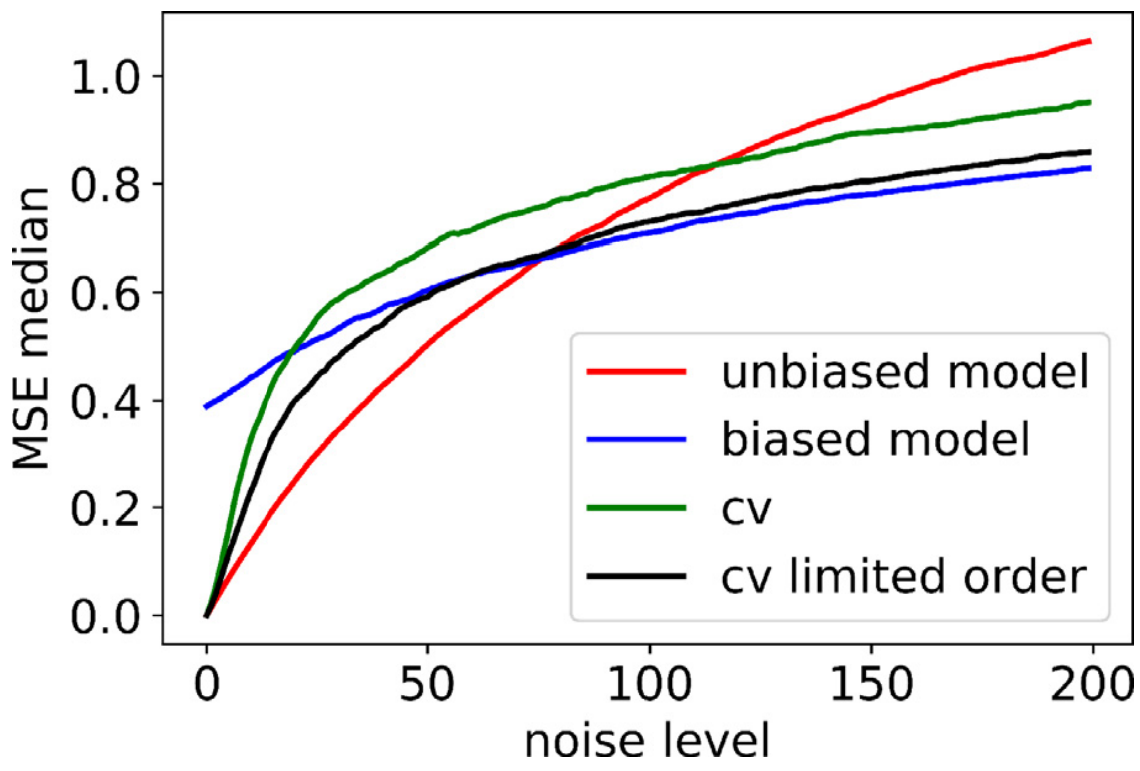
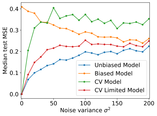
Figure 2: Test set median MSE for the “4th-degree, univariate polynomial” dataset. ALVEN results (left, reproduced from Sun & Braatz (2021) with permission) show that the error is monotonically increasing with noise and that the degree 4 “unbiased model” is the best at low noise levels, but is displaced by the degree 2 “biased model” at higher noise levels. On the other hand, LCEN results (right) show that the median errors converge at higher noises. Furthermore, the LCEN median errors are typically over 60% smaller than the ALVEN median errors, and the degree 4 “unbiased model” is always the best model no matter the noise. The “noise level” and “Noise variance $\sigma^{2}$” terms are equivalent in this figure.

3.2 Empirical data from processes with known physical laws further highlight LCEN’s feature selection potential

The applicability of an algorithm to real-world problems is judged only by its performance on real data, as data sparsity or noise may affect the algorithm’s capabilities. These tests are summarized in Table A3. The first test uses the “CARMENES star data” dataset from Schweitzer et al. (2019). This dataset contains information on temperature ($T$), radius ($R$), and luminosity ($L$) of 293 white dwarf stars. These features are linked together by the Stefan-Boltzmann equation, $L=4\pi R^{2}\sigma T^{4}$, where $\sigma$ is a constant. Normalizing this equation to values from another star (typically, the Sun), conveniently sets the constant terms to 1. This normalization is applied to the “CARMENES star data” dataset. LCEN with degrees from 1 to 10 was applied to this normalized dataset. Despite the very large number of potential features (due to the high degree values used), LCEN correctly selected only the $R^{2}T^{4}$ feature. The coefficient assigned to $R^{2}T^{4}$ is 0.9826, which is well within the 2–3% error on these data (as reported by Schweitzer et al. (2019)). LCEN retained high performance for this real data in a high-hyperparameter variance scenario.

A potential limitation in real datasets is data scarcity. To evaluate the LCEN algorithm in a low-data scenario, the “Kepler’s 3rd Law” datasets are created. The first version uses the original data obtained by Kepler, first published in 1619 and republished in Kepler et al. (1997). From only 6 (slightly inaccurate) measurements, Kepler was able to derive the eponymous Kepler’s 3rd law, which states that the period $T$ of a celestial body is related to the semi-major axis of its orbit $a$ by $T=ka^{3/2}$. The constant $k$ depends on the masses of the central and orbiting bodies; however, as the mass of the central body is typically much larger, the mass of the orbiting body is ignored. In this and Kepler’s works, $T$ is measured in Earth days, so the constant $k$ is $\sim$365.25 when using modern data and $\sim$365.15 when using Kepler’s original data. Despite the low number of data points, LCEN correctly selected only the $a^{3/2}$ feature. Moreover, the coefficient assigned to that feature was 366.82, an error of only 0.46% relative to Kepler’s $k=365.15$.

LCEN is then evaluated using a modern version of the same dataset, which contains 8 points (as Uranus and Neptune were discovered after Kepler’s observations) whose data were measured with greater accuracy. On this modern “Kepler’s 3rd Law” dataset, LCEN again selects only the $a^{3/2}$ feature. The coefficient assigned to the $a^{3/2}$ feature is 365.00, an error of only 0.07% relative to the modern value $k=365.25$. LCEN did perfect feature selection in these data-scarce scenarios, with parameter estimates minimally affected by experimental noise.

Lastly, LCEN is tested on the “Newton’s Law of Cooling” dataset to determine its ability to work with scarce, time-series data approximated from a differential equation. This dataset was published by Newton (1701) and republished in English by Simms (2004). Newton used 14 measurements to determine the cooling rate of a “pretty thick piece of red-hot iron” (Simms, 2004). While Newton made some improper assumptions in that work (including ignoring thermal radiation emissions, which are calculated through the Stefan-Boltzmann equation), his measurements are accurate for $T\leq 300^{\circ}$C (Simms, 2004). In its non-dimensionalized form, Newton’s Law of Cooling relates the rate of change of temperature of an object to its temperature $T(t)$ and the temperature of its surroundings $T_{\text{env}}$, such that $\frac{dT}{dt}=rT_{\text{env}}-rT(t)$. The constant $r$ is the heat transfer coefficient which depends on the object’s mass, surface area $A_{s}$, specific heat capacity $c_{p}$, and fluid heat transfer coefficient $h$, such that $r=\frac{hA_{s}}{mc_{p}}$. Applying a first-order finite difference approximation and rearranging replaces Newton’s Law of Cooling by $T(t)=rT_{\text{env}}\Delta t+T(t-1)(1-r\Delta t)$.

LCEN correctly selected only the $T(t-1)$ feature. The intercept ($rT_{\text{env}}\Delta t$) was not selected, which may be explained by the low $T_{\text{env}}=10^{\circ}C$ during Newton’s experiments and by how $r\Delta t\ll 1$. The coefficient assigned to the $T(t-1)$ feature is 0.9732. As the average $\Delta t=9.4$ min, this implies $r=2.84$$\times$$10^{-3}\,\frac{1}{s}$. As Newton did not provide information on the surface area of his iron, it is impossible to perfectly validate this number. However, estimates can show that this value of $r$ is realistic. The mass of the iron block used by Newton was 4.25 lb avoirdupois (Simms, 2004), equivalent to 1.93 kg. The density of iron is 7.874 $\frac{\text{g}}{\text{cm}^{3}}$, which implies a volume of 244.8 cm³, and its specific heat capacity is $449\,\frac{\text{J}}{\text{kg}^{\circ}\text{C}}$ (The Engineering ToolBox, 2003). For forced convection with air, $h\approx 100\frac{\text{W}}{\text{m}^{2}\text{K}}$. Thus, the surface area $A_{s}$ is $\sim$246.1 cm². Assuming that Newton’s iron block was a rectangular cuboid, a block with dimensions 12$\times$6$\times$3.4 cm, which follows the Good Delivery dimension specifications for a half-length but thick gold bar (London Bullion Market Association, 2024), would have the correct volume and surface area. Thus, the coefficient found by LCEN is realistic.

3.3 LCEN surpasses many other models when making predictions on empirical data from processes with unknown physical laws

The final experiments to validate LCEN’s performance involve comparisons to other algorithms on real datasets from processes with unknown physical laws. As there is no (computational) way to validate the feature selection by models trained on these datasets, the main focuses of this section are investigating prediction errors and sparsities of different model architectures.

The first dataset analyzed is the “Diesel Freezing Point” dataset (Hutzler & Westbrook, 1999), which is comprised of 395 diesel spectra measured at 401 wavelengths and used to predict the freezing point of these diesels. LCEN; the dense model architectures of ordinary least squares (OLS), ridge regression (RR), and partial least squares (PLS); and the sparse model architectures LASSO and EN are compared in Table 3. Most models had test set RMSEs slightly smaller than 5.0^∘C, which is about 7.5% of the range of the test data, which contains diesels with freezing points between $-59.5^{\circ}$C and $6.6^{\circ}$C. RR and EN had the lowest test RMSEs of 4.83^∘C, and LCEN followed right after with a test RMSE of $4.86^{\circ}$C. However, the best hyperparameters for EN included an l1_ratio = 0.1, which makes its model very dense. Whereas RR selected all 401 features and EN selected 299, LCEN was able to achieve similar performance with only 37 features. Moreover, LCEN is also faster: whereas EN took 19.6 s to run, LCEN took only 6.82 s. Finally, the LCEN cutoff hyperparameter was increased from the value that minimizes the validation MSE to create sparser models. These models have much fewer variables, yet their test set RMSEs increase by less than 1^∘C. This illustrates how LCEN can select the most critical features to make models with high sparsity and predictive power, and how these criteria can be prioritized by the end-user.

Table 3: Results of different model architectures for the “Diesel Freezing Point” dataset.

Architecture Test RMSE (^∘C) Features Runtime (s) OLS 11.75 401 0.09 PLS 5.21 401 4.44 RR 4.83 401 4.87 EN 4.83 299 19.6 LASSO 4.90 39 2.06 LCEN 4.86 37 6.82 4.95 20 6.43 5.16 10 6.02 5.47 5 5.82 5.80 3 5.85

The next dataset used is the “Abalone” dataset (Nash et al., 1995). Abalone (Haliotis sp.) are sea snails whose age can be determined by cutting their shells, staining them, and counting the stained shell rings under a microscope. This process is laborious and error-prone. An alternative is to estimate the number of rings based on readily available physical characteristics, such as weight and size. As before, LCEN was compared with other dense and sparse machine learning models, and LCEN models with increased sparsity were also generated (Table 4). In this problem, OLS, RR, LASSO, and EN all converged to the OLS solution (that is, no regularization), selecting all 9 linear features and having an RMSE of 2.1 rings. On the other hand, LCEN automatically detected that 2nd degree features would be relevant. The model with the LCEN algorithm selected 11 features (both 1st- and 2nd-degree features) and had an RMSE of 2.0 rings. By increasing the sparsity, an LCEN model with only 3 features (one of which was a 2nd-degree feature) had an RMSE of 2.2 rings. This experiment further illustrates LCEN’s selecting the best features even when hyperparameter variance is present, and very sparse LCEN models retaining significant performance.

Table 4: Results of different model architectures for the “Abalone” dataset.

Architecture Test RMSE (rings) Features OLS=RR=LASSO=EN 2.1 9 LCEN 2.0 11 2.2 3

LCEN is then tested on the “Concrete Compressive Strength” dataset (Yeh, 1998), which contains the composition and age of 1,030 different types of concrete and their compressive strengths. The relationship between these properties is nonlinear, and previous modeling attempts include algebraic expressions and artificial neural networks (Yeh, 1998, 2006). These ANNs were superior to the algebraic models, whereas the algebraic models provide interpretability on how the properties of the concrete affect its compressive strength. LCEN is also considerably better than the previously published algebraic models (Table 5), and its performance is competitive with that of previously published ANNs without sacrificing interpretability. Furthermore, note that no type of validation is mentioned in Yeh (1998), so the test and validation sets may be the same, making the ANN figures overoptimistic. LCEN has a validation RMSE of 4.78 MPa and an $R^{2}$ of 0.920 on this dataset, which are effectively equal to those from the ANN of Yeh (1998).

Table 5: Results of different model architectures for the “Concrete Compressive Strength” dataset. No type of validation is mentioned in Yeh (1998), so the test and validation sets may be the same, making the ANN values overoptimistic.

Architecture Test RMSE (MPa) Test R² Algebraic expression (Yeh, 1998) 7.79 0.770 ANN (Yeh, 1998) 4.76 0.914 Linear + interactions model (Yeh, 2006) 7.43 0.791 LCEN (this work) 5.82 0.872

4 Discussion

This work introduces the LASSO-Clip-EN (LCEN) algorithm for the creation of nonlinear, interpretable machine learning models (Algorithm 1). The algorithm is first validated using artificial data (Section 3.1), which provide an initial assessment of the algorithm’s performance under different conditions, which can be controlled independently. LCEN displayed high performance for data that are noisy (“Linear, 5-variable polynomial” and “4th-degree, univariate polynomial” datasets; Table 1 and Fig. 2), multicollinear (“Multicollinear data” dataset; Fig. 1), or generated from a process with a complex nonlinear function (“Relativistic energy” and “4th-degree, univariate polynomial” datasets; Table 2 and Fig. 2), which also leads to high hyperparameter and feature variance. For the “4th-degree, univariate polynomial” dataset, LCEN automatically adjusted its predictions to compensate for the bias-variance tradeoff (Figs. 2 and A1). During the experiments with the “Relativistic energy” dataset, the range of the data affected the prediction performance – data with higher ranges led to more accurate predictions even at high noises. We hypothesize that this phenomenon occurs because it is difficult to distinguish between multiple powers of a variable (or, in a more generalized manner, how Taylor approximations are successful) when the data cover low ranges and are noisy.

LCEN was then tested with data from processes with known physical laws (Section 3.2). These data have real properties (such as noise) and may have limitations common to many processes (such as low amounts of data). Nevertheless, LCEN successfully selected the correct features for all datasets used in this work, effectively rediscovering physical laws solely from data (Table A3). The first dataset tested was the “CARMENES star data”, which contains hundreds of points described by Stefan-Boltzmann law. This law uses a 6th-order interaction, but since this would not be known a priori, LCEN was tested using all degree hyperparameters from 1 to 10. Despite the high variance of the process and the many potential features that could be selected, LCEN selected only the correct $R^{2}T^{4}$ feature with a coefficient relative error of only 1.74%, which is well within the 2–3% data error. Next, LCEN was evaluated for the “Kepler’s 3rd Law” datasets, which contain small amounts of data (only 6 or 8 points) yet were enough for Kepler to derive the eponymous law in 1619. LCEN can automatically replicate this discovery despite the slightly inaccurate data from Kepler’s measurements, selecting only the correct $a^{3/2}$ feature. The coefficient relative errors were 0.46% on Kepler’s original data and 0.07% on modern data, extremely small values that highlight the algorithm’s accuracy. LCEN algorithm was also demonstrated for (scarce) time-series data, to model the “Newton’s Law of Cooling” dataset. LCEN again discovered the correct features (although a very small intercept was ignored), and the predicted coefficients were realistic according to estimations.

Lastly, experiments using empirical data from processes with unknown laws further validated LCEN’s feature selection and predictive performance. LCEN was compared to multiple different model architectures, including LASSO, EN, and ANNs. On the “Diesel Freezing Point” dataset (Table 3), LCEN had a test RMSE within 1% of the RMSEs for RR and EN, which tied for the lowest RMSE. However, LCEN required 10.8 and 8.1 times fewer features than RR and EN (respectively) to reach the same accuracy, and LCEN was 2.9-fold faster than EN. LCEN also generated a more accurate and sparser model than LASSO, and LCEN models with increased sparsities displayed only small increases in the prediction error. In the most extreme case, an LCEN model that used only 3/401 features had a test RMSE less than 1^∘C larger than the best models. LCEN provided a combination of accuracy, sparsity/interpretability, and speed that was unmatched by the traditional dense and sparse linear machine learning methods. On the “Abalone” dataset (Table 4), LCEN automatically recognized the importance of 2nd-degree features, which led to its producing the model with the lowest RMSE. OLS, RR, LASSO, and EN converged to the same dense linear model. Similarly to what happened with the “Diesel Freezing Point” dataset, an LCEN model using only 3 features, one of which was 2nd-degree, displayed only a 2.2% increase in RMSE relative to the dense models. As before, LCEN built very sparse yet very accurate models. Finally, LCEN was compared to an algebraic expression, a machine learning model, and an ANN on the “Concrete Compressive Strength” dataset (Table 5). LCEN displayed a test RMSE at least 22% lower than that of the other interpretable models and produces a model that is simpler and interpretable while having an RMSE competitive with that of the ANN. Yeh (1998), the paper that originated the ANN, does not mention any type of validation, which could indicate that the ANN results are overoptimistic. The validation performance of LCEN was equal to the ANN test performance reported in Yeh (1998), indicating LCEN is competitive even with ANNs on this problem if the results reported by Yeh (1998) are actually validation results.

Overall, these experiments have demonstrated the applicability of LCEN to a multitude of scientific problems. The models trained by LCEN were robust to defects in the real data, including noise, multicollinearity, or sample scarcity. LCEN models were as accurate as or more accurate than many alternative architectures, yet were also much sparser. This combination of accuracy and interpretability is essential for the deployment of machine-learning models in performance-critical scenarios, from aviation to medicine. LCEN is free, open-source, and easy to use, allowing even non-specialists in machine learning to benefit from the algorithm and use it in technical work. Moreover, the additional interpretability can assist in data or model refinement efforts and can make the models robust to changes in data or adversarial input. Finally, this mathematical, feature-based algorithm can also be used to automate efforts in certain hybrid model architectures (such as physics-constrained or physics-guided ML).

Impact Statement

The main societal impact of this paper is the creation of interpretable and accurate machine learning models. These may increase the robustness, trust, and reliability of ML models applied in many scenarios, including performance-critical scenarios such as aviation and medicine. A discussion of the benefits of interpretability is beyond the scope of this section; many other works have been dedicated to this, such as Rudin (2019).

A1 Appendix – Datasets

The “Linear, 5-variable polynomial” dataset was created by drawing numbers from a uniform distribution between 1 and 10 and summing, potentially adding noise, such that $y=-2.8X_{0}-2.7X_{1}-5.3X_{2}+4.3X_{3}+9.0X_{4}+\epsilon$. The “Multicollinear data” dataset was created by drawing numbers from a uniform distribution between 1 and 10 to create one variable $X_{0}$, which was used together with a small amount of noise to create a correlated variable $X_{1}=X_{0}+\epsilon_{1}$; finally, they were summed such that $y=2X_{0}+2X_{1}+\epsilon_{2}$. The “Relativistic energy” dataset was created by drawing numbers from a uniform distribution between 1 and 10 or 1 and 100 for masses, and 5$\times$10⁷ and 2.5$\times$10⁸ for velocities, which represent the energy of a body as $E^{2}=c^{4}m^{2}+c^{2}m^{2}v^{2}$. With these velocity numbers, relativistic effects are responsible for 20.4% of the total squared energy on average. The “4th-degree, univariate polynomial” dataset was created by drawing numbers from a normal distribution with mean 0 and variance 5; these numbers were transformed into the polynomial $y=X+0.5X^{2}+0.1X^{3}+0.05X^{4}+\epsilon$.

The real datasets are described in the main text (Sections 3.2 and 3.3).

Table A1: Datasets used in this work and their sources. The artificial datasets are used in Section 3.1; the real datasets from processes with known physical laws are used in Section 3.2; and the real datasets from processes with unknown physical laws are used in Section 3.3.

Dataset Name Source Linear, 5-variable polynomial Artificial data generated by us Multicollinear data Artificial data generated by us Relativistic energy Artificial data generated by us 4th-degree, univariate polynomial Artificial data generated by us CARMENES star data (Schweitzer et al., 2019) [link to dataset] Kepler’s 3rd Law (Kepler et al., 1997) (Original from 1619) (Wolfram Alpha LLC, 2022) (Modern) Newton’s Law of Cooling (Newton, 1701); translated by Simms (2004) Diesel Freezing Point (Hutzler & Westbrook, 1999) [link to dataset] Abalone (Nash et al., 1995) Concrete Compressive Strength (Yeh, 1998) [dataset: (Yeh, 2007)]

A2 Appendix – The degree hyperparameter of the LCEN algorithm

Table A2: Additional features included for each value of the degree hyperparameter for a dataset with features $X_{0}$, $X_{1}$, and $X_{2}$. A degree of $n$ (any natural number) includes all features from degrees 1 to $n-1$.

Degree Sample new features included [for all $k$] Number of features 1 intercept, $X_{k},\ln X_{k},({X_{k}})^{1/2},{1}/{X_{k}}$ 13 2 $(X_{k})^{2},X_{0}X_{1},X_{0}X_{2},X_{1}X_{2},(\ln X_{k})^{2},(X_{k})^{3/2},\frac{1}{(X_{k})^{2}},\frac{\ln{X_{k}}}{X_{k}}$ 37 3 $(X_{k})^{3},X_{0}X_{1}X_{2},(X_{0})^{2}X_{1},X_{1}(X_{2})^{2},(\ln X_{k})^{3},(X_{k})^{5/2},\frac{1}{(X_{k})^{3}},\frac{\ln(X_{k})^{2}}{X_{k}},\frac{\ln(X_{k})}{(X_{k})^{2}}$ 75 4 […] 129 5 […] 201

A3 Appendix – Additional results

Table A3: Summary of LCEN results for the empirical datasets from processes with known physical laws.

Dataset Correct Equation Rel. Error CARMENES star data Yes 1.74% Kepler’s 3rd Law (1619) Yes 0.46% Kepler’s 3rd Law (Modern) Yes 0.07% Newton’s Law of Cooling Yes, no intercept N/A

Figure A1: Degrees selected by the model with a degree between 1 and 10 “cv” trained using the LCEN algorithm. At lower noise levels (noise variance $\sigma^{2}\leq 30$), LCEN tends to primarily select degree = 4. At higher noise levels, there is a shift to primarily select degree = 2.

References

- Akaike (1974) Akaike, H. A new look at the statistical model identification. IEEE Transactions on Automatic Control, 19(6):716–723, 1974. URL https://doi.org/10.1109/TAC.1974.1100705.
- Brewick et al. (2017) Brewick, P. T., Masri, S. F., Carboni, B., and Lacarbonara, W. Enabling reduced-order data-driven nonlinear identification and modeling through naïve elastic net regularization. International Journal of Non-Linear Mechanics, 94:46–58, 2017. URL https://doi.org/10.1016/j.ijnonlinmec.2017.01.016.
- Clark et al. (1996) Clark, D., Schreter, Z., and Adams, A. A quantitative comparison of dystal and backpropagation. In Proceedings of the Seventh Australian Conference on Neural Networks, pp. 132–137, 1996. URL https://www.tib.eu/de/suchen/id/BLCP%3ACN016972815.
- Dalalyan et al. (2017) Dalalyan, A. S., Hebiri, M., and Lederer, J. On the prediction performance of the Lasso. Bernoulli, 23(1):552 – 581, 2017. URL https://doi.org/10.3150/15-BEJ756.
- Hebiri & Lederer (2013) Hebiri, M. and Lederer, J. How correlations influence lasso prediction. IEEE Transactions on Information Theory, 59(3):1846–1854, 2013. URL https://doi.org/10.1109/TIT.2012.2227680.
- Heinze et al. (2018) Heinze, G., Wallisch, C., and Dunkler, D. Variable selection – A review and recommendations for the practicing statistician. Biometrical Journal, 60(3):431–449, 2018. URL https://doi.org/10.1002/bimj.201700067.
- Hong et al. (2020) Hong, S. R., Hullman, J., and Bertini, E. Human factors in model interpretability: Industry practices, challenges, and needs. Proceedings of the ACM on Human-Computer Interaction, 4(CSCW1), May 2020. URL https://doi.org/10.1145/3392878.
- Hutzler & Westbrook (1999) Hutzler, S. A. and Westbrook, S. R. Estimating chemical and bulk properties of middle distillate fuels from near-infrared spectra. Defense Technical Information Center, 1999. URL https://apps.dtic.mil/sti/citations/ADA394209.
- Kepler et al. (1997) Kepler, J., Aiton, E., Duncan, A., and Field, J. The Harmony of the World, pp. 418, 422. American Philosophical Society, 1997. URL https://books.google.com/books?id=rEkLAAAAIAAJ.
- London Bullion Market Association (2024) London Bullion Market Association. Good delivery rules – Technical specifications, 2024. URL https://www.lbma.org.uk/publications/good-delivery-rules/technical-specifications.
- McConaghy (2011) McConaghy, T. FFX: Fast, Scalable, Deterministic Symbolic Regression Technology, pp. 235–260. Springer, New York, 2011. URL https://doi.org/10.1007/978-1-4614-1770-5_13.
- Nash et al. (1995) Nash, W., Sellers, T., Talbot, S., Cawthorn, A., and Ford, W. Abalone. UCI Machine Learning Repository, 1995. URL https://doi.org/10.24432/C55C7W.
- Newton (1701) Newton, I. VII. Scala graduum caloris. Philosophical Transactions of the Royal Society of London, 22:824–829, 1701. URL https://doi.org/10.1098/rstl.1700.0082.
- Pavlou et al. (2016) Pavlou, M., Ambler, G., Seaman, S., De Iorio, M., and Omar, R. Z. Review and evaluation of penalised regression methods for risk prediction in low-dimensional data with few events. Statistics in Medicine, 35(7):1159–1177, 2016. URL https://doi.org/10.1002/sim.6782.
- Ribeiro et al. (2016) Ribeiro, M. T., Singh, S., and Guestrin, C. Model-agnostic interpretability of machine learning. In ICML Workshop on Human Interpretability in Machine Learning, pp. 91–95, 2016. URL https://arxiv.org/abs/1606.05386.
- Rudin (2019) Rudin, C. Stop explaining black box machine learning models for high stakes decisions and use interpretable models instead. Nature Machine Intelligence, 1:206–215, 2019. URL https://doi.org/10.1038/s42256-019-0048-x.
- Santosa & Symes (1986) Santosa, F. and Symes, W. W. Linear inversion of band-limited reflection seismograms. SIAM Journal on Scientific and Statistical Computing, 7(4):1307–1330, 1986. URL https://doi.org/10.1137/0907087.
- Schwarz (1978) Schwarz, G. Estimating the dimension of a model. The Annals of Statistics, 6(2):461–464, 1978. URL https://doi.org/10.1214/aos/1176344136.
- Schweitzer et al. (2019) Schweitzer, A., Passegger, V. M., Cifuentes, C., Béjar, V. J. S., Cortés-Contreras, M., Caballero, J. A., del Burgo, C., Czesla, S., Kürster, M., Montes, D., Zapatero Osorio, M. R., Ribas, I., Reiners, A., Quirrenbach, A., Amado, P. J., Aceituno, J., Anglada-Escudé, G., Bauer, F. F., Dreizler, S., Jeffers, S. V., Guenther, E. W., Henning, T., Kaminski, A., Lafarga, M., Marfil, E., Morales, J. C., Schmitt, J. H. M. M., Seifert, W., Solano, E., Tabernero, H. M., and Zechmeister, M. The CARMENES search for exoplanets around M dwarfs. Different roads to radii and masses of the target stars. Astron. Astrophys., 625:A68, May 2019. URL https://doi.org/10.1051/0004-6361/201834965.
- Shmueli (2010) Shmueli, G. To explain or to predict? Statistical Science, 25(3):289–310, 2010. URL https://doi.org/10.1214/10-STS330.
- Simms (2004) Simms, D. L. Newton’s contribution to the science of heat. Annals of Science, 61(1):33–77, 2004. URL https://doi.org/10.1080/00033790210123810.
- Smith (2018) Smith, G. Step away from stepwise. Journal of Big Data, 5:32, 2018. URL https://doi.org/10.1186/s40537-018-0143-6.
- Sun & Braatz (2020) Sun, W. and Braatz, R. D. ALVEN: Algebraic learning via elastic net for static and dynamic nonlinear model identification. Computers & Chemical Engineering, 143:107103, 2020. URL https://doi.org/10.1016/j.compchemeng.2020.107103.
- Sun & Braatz (2021) Sun, W. and Braatz, R. D. Smart process analytics for predictive modeling. Computers & Chemical Engineering, 144:107134, 2021. URL https://doi.org/10.1016/j.compchemeng.2020.107134.
- The Engineering ToolBox (2003) The Engineering ToolBox. Specific heat of common substances, 2003. URL https://www.engineeringtoolbox.com/specific-heat-capacity-d_391.html.
- Tian et al. (2015) Tian, S., Yu, Y., and Guo, H. Variable selection and corporate bankruptcy forecasts. Journal of Banking & Finance, 52:89–100, 2015. URL https://doi.org/10.1016/j.jbankfin.2014.12.003.
- Waugh (1995) Waugh, S. Extending and Benchmarking Cascade-Correlation: Extensions to the Cascade-Correlation Architecture and Benchmarking of Feed-forward Supervised Artificial Neural Networks. PhD thesis, University of Tasmania, 1995. URL https://api.semanticscholar.org/CorpusID:53803349.
- Whittingham et al. (2006) Whittingham, M. J., Stephens, P. A., Bradbury, R. B., and Freckleton, R. P. Why do we still use stepwise modelling in ecology and behaviour? Journal of Animal Ecology, 75(5):1182–1189, 2006. URL https://doi.org/10.1111/j.1365-2656.2006.01141.x.
- Wolfram Alpha LLC (2022) Wolfram Alpha LLC. Wolfram|Alpha, 2022.
- Yeh (1998) Yeh, I.-C. Modeling of strength of high-performance concrete using artificial neural networks. Cement and Concrete Research, 28(12):1797–1808, 1998. URL https://doi.org/10.1016/S0008-8846(98)00165-3.
- Yeh (2006) Yeh, I.-C. Analysis of strength of concrete using design of experiments and neural networks. Journal of Materials in Civil Engineering, 18(4):597–604, 2006. URL https://doi.org/10.1061/(ASCE)0899-1561(2006)18:4(597).
- Yeh (2007) Yeh, I.-C. Concrete Compressive Strength. UCI Machine Learning Repository, 2007. URL https://doi.org/10.24432/C5PK67.
- Zou & Hastie (2005) Zou, H. and Hastie, T. Regularization and Variable Selection Via the Elastic Net. Journal of the Royal Statistical Society Series B: Statistical Methodology, 67(2):301–320, 2005. URL https://doi.org/10.1111/j.1467-9868.2005.00503.x.