Diffusion Posterior Proximal Sampling for Image Restoration

Abstract

Diffusion models have demonstrated remarkable efficacy in generating high-quality samples. Existing diffusion-based image restoration algorithms exploit pre-trained diffusion models to leverage data priors, yet they still preserve elements inherited from the unconditional generation paradigm. These strategies initiate the denoising process with pure white noise and incorporate random noise at each generative step, leading to over-smoothed results. In this paper, we introduce a refined paradigm for diffusion-based image restoration. Specifically, we opt for a sample consistent with the measurement identity at each generative step, exploiting the sampling selection as an avenue for output stability and enhancement. Besides, we start the restoration process with an initialization combined with the measurement signal, providing supplementary information to better align the generative process. Extensive experimental results and analyses validate the effectiveness of our proposed approach across diverse image restoration tasks.

1 Introduction

Figure 1: Examples of the super-resolution ($\times$4) task to illustrate the efficiency of our method, where $n$ denotes the number of candidate samples, and DPS also refers to the case where $n=1$. Additional results are presented in Appendix F.

Figure 2: High-level illustration of our proposed DPPS ($n$=2). Existing methods employ random sampling from the predicted distribution, our approach takes multiple samples and selecting the one with better data consistency (denoted by $\checkmark$) at each step.

Diffusion models (Vincent, 2011; Ho et al., 2020; Song et al., 2021b) have gained broad attention due to the powerful ability to model complex data distribution, and have been applied to a wide range of tasks such as image generation (Dhariwal & Nichol, 2021; Meng et al., 2021; Rombach et al., 2022), molecule generation (Corso et al., 2023), and natural language processing (Li et al., 2022). Recent research has demonstrated that pre-trained unconditional diffusion models can be effectively employed to address image restoration problems (Song et al., 2022; Kawar et al., 2022; Chung et al., 2022; Wang et al., 2023; Song et al., 2023b) to leverage rich priors in a plug-and-play fashion, and achieve significant advancements.

However, for diffusion-based image restoration algorithms, they still retain a process inherited from unconditional generation. In particular, (i) these methods start generating the image that corresponds to the measurement with a white noise as initialization, and (ii) a fully stochastic noise is introduced at each step of the generation process. We argue that this paradigm is inappropriate for solving image restoration tasks. Firstly, randomness enriches the diversity of the generated samples in unconditional generation (Liu et al., 2020; Xiao et al., 2021). However, for image restoration tasks where the identity information of the measurement needs to be preserved, randomness leads to uncontrollable generation outcomes (Cao et al., 2023). Secondly, in the generative process of diffusion-based model, the current state is randomly sampled (Chung et al., 2023a; Song et al., 2023b) from the predicted distribution without any correction. Considering the Markovian reverse process, the sampling quality of the next state heavily depends on the current sampling result. If the current result deviates considerably from expectations, the subsequent generative process will encounter a significant exposure bias problem (Ning et al., 2023; Li et al., 2023). As a consequence, randomness introduces fluctuations and instability into the generative process, ultimately leading to over-smoothed results.

In this paper, we advance toward a more refined paradigm for solving image inverse problems with pre-trained diffusion models. Specifically, to ensure the sampling result is closely consistent with the measurement identity, we opt for the proximal sample at each step from multiple candidate samples, as opposed to making a random choice. By mitigating uncertainties, the sample consistently progresses toward the desired targets, resulting in a stable generative process and improved output quality. Moreover, we start the generation process with an initialization composed of both the measurement signal and white noise, rather than pure white noise. Consequently, the denoising process commences from a closer starting point, facilitating a faster convergence toward the desired result.

We theoretically analyze that our approach reduces variance in comparison to existing state-of-the-art methods which introduce random sampling. And we conduct extensive experiments to demonstrate the superior restoration capabilities of our method across diverse image restoration tasks, such as super-resolution (SR), deblurring, and inpainting, with only a marginal additional cost. Furthermore, sufficient experimental analyses are shown to validate the effectiveness of our proposed strategy.

In summary, our contributions are as follows:

• We pioneer to improve the generation quality by exploiting sampling choice from the predicted distribution of each reverse step.

• We introduce an efficient proximal sampling strategy that aligns with measurement identity to solve diffusion-based image restoration problems.

• Extensive experiments are conducted to demonstrate our superior performance in image restoration tasks, and abundant ablation analysis verifies the validity of the proposed method.

2 Background

2.1 Denoising Diffusion Probabilistic Models

Denoising Diffusion Probabilistic Models (DDPMs) (Ho et al., 2020) is a class of models that incorporate a forward (diffusion) process and a corresponding reverse (generative) process. Consider a $T$-step forward process, the noised sample $\mathbf{x}_{t}$ at time step $t$ can be modeled from the previous state $\mathbf{x}_{t-1}$:

$$q(\mathbf{x}_{t}|\mathbf{x}_{t-1})=\mathcal{N}(\mathbf{x}_{t};\sqrt{1-\beta_{t}}\mathbf{x}_{t-1},\beta_{t}\mathbf{I}),$$ (1)

where $\mathcal{N}$ denotes the Gaussian distribution, and $\beta_{t}$ is a pre-defined parameter increasing with $t$. Through reparameterization, $\mathbf{x}_{t}$ satisfies the following conditional distribution $q(\mathbf{x}_{t}|\mathbf{x}_{0})=\mathcal{N}(\mathbf{x}_{t};\sqrt{\bar{\alpha}_{t}}\mathbf{x}_{0},(1-\bar{\alpha}_{t})\mathbf{I})$, where $\bar{\alpha}_{t}=\prod_{i=0}^{t}\alpha_{i}$ and $\alpha_{t}=1-\beta_{t}$.

On the other hand, the reverse process of DDPM is formulated by the transition kernel parameterized by $\mathbf{\theta}$:

$$p_{\mathbf{\theta}}(\mathbf{x}_{t-1}|\mathbf{x}_{t})=\mathcal{N}(\mathbf{x}_{t-1};\bm{\mu}_{\mathbf{\theta}}(\mathbf{x}_{t},t),\sigma_{t}\mathbf{I}).$$ (2)

where the learning objective aims to minimize the KL divergence between the forward and backward processes. The epsilon-matching objective is typically set as:

$$\mathbf{L}({\mathbf{\theta}})=\mathbb{E}_{\mathbf{x}_{0}\sim q(\mathbf{x}_{0}),{\bm{\epsilon}}\sim{\cal N}(\mathbf{0},\mathbf{I}),t\sim\mathbb{U}(\{1,...,T\})}[\|{\bm{\epsilon}}-{\bm{\epsilon}}_{\mathbf{\theta}}(\mathbf{x}_{t},t)\|^{2}].$$ (3)

where $\mathbf{x}_{0}$ is sampled from training data and $\mathbf{x}_{t}\sim q(\mathbf{x}_{t}|\mathbf{x}_{0})$. Once we have access to the well-trained $\bm{\epsilon}_{\mathbf{\theta}}(\mathbf{x}_{t},t)$, a clean sample can be derived by evaluating the generative reverse process Eq. (2) step by step.

Furthermore, one can view the DDPM equivalent to the variance preserving (VP) form of the stochastic differential equation (SDE) (Song et al., 2021b). Accordingly, the epsilon-matching objective Eq. (3) is equivalent to the denoising score-matching (Sohl-Dickstein et al., 2015) objective with different parameterization:

$$\mathbf{L}({\mathbf{\theta}})=\mathbb{E}_{\mathbf{x}_{0},{\bm{\epsilon}},t}[||\mathbf{s}_{{\mathbf{\theta}}}(\mathbf{x}_{t},t)-\nabla_{\mathbf{x}_{t}}\log q(\mathbf{x}_{t}|\mathbf{x}_{0})||^{2}].$$ (4)

Algorithm 1 DPS

0:  $T$, $\mathbf{y}$, {$\lambda_{t}\}_{t=1}^{T}$, ${\{\sigma_{t}\}_{t=1}^{T}}$

1:  $\mathbf{x}_{T}\sim\mathcal{N}(\mathbf{0},\mathbf{I})$

2:  for $t=T$ to $1$ do

3:     compute $\bm{\mu}_{\mathbf{\theta}}(\mathbf{x}_{t},t,\mathbf{y})$ via (8)

4:     if $t>1$ then ${\mathbf{z}}_{t}\sim{\mathcal{N}}(\mathbf{0},\mathbf{I})$, else $\mathbf{z}_{t}=\mathbf{0}$

5:     $\mathbf{x}_{t-1}\leftarrow\bm{\mu}_{\mathbf{\theta}}(\mathbf{x}_{t},t,\mathbf{y})+\sigma_{t}{\mathbf{z}}_{t}$

6:  end for

7:  return $\hat{\mathbf{x}}_{0}$

2.2 Diffusion Based Solvers for Image Restoration

This paper focuses on solving the image restoration, or image inverse problems with unconditional diffusion model (Kawar et al., 2022; Chung et al., 2023a; Song et al., 2023b). Our goal is to retrieve the unknown $\mathbf{x}_{0}$ from a degraded measurement $\mathbf{y}$:

$$\mathbf{y}=\mathcal{A}(\mathbf{x}_{0})+\mathbf{n},\quad\mathbf{y},\mathbf{n}\in{\mathbb{R}}^{n},\,\mathbf{x}\in{\mathbb{R}}^{d},$$ (5)

where $\mathcal{A}(\cdot):{\mathbb{R}}^{d}\mapsto{\mathbb{R}}^{n}$ is the degradation operator and $\mathbf{n}\sim\mathcal{N}(\mathbf{0},{\sigma_{y}^{2}}\mathbf{I})$ denotes the measurement noise. The restoration problem can be addressed via conditional diffusion models by substituting the score function $\nabla_{\mathbf{x}_{t}}\log(\mathbf{x}_{t})$ in the reverse-time SDE with the conditional score function $\nabla_{\mathbf{x}_{t}}\log(\mathbf{x}_{t}|\mathbf{y})$, which can be derived by Bayes’ rule:

$$\nabla_{\mathbf{x}_{t}}\log p_{t}(\mathbf{x}_{t}|\mathbf{y})=\nabla_{\mathbf{x}_{t}}\log p_{t}(\mathbf{x}_{t})+\nabla_{\mathbf{x}_{t}}\log p_{t}(\mathbf{y}|\mathbf{x}_{t}).$$ (6)

The first prior term can be approximated by a well-trained score network. However, the analytic solution of the second likelihood term is computationally intractable, since there only exists an explicit connection between $\mathbf{y}$ and $\mathbf{x}_{0}$. To solve this dilemma, Chung et al. (2023a) propose diffusion posterior sampling (DPS) to approximate the likelihood using a Laplacian approximation: $\nabla_{\mathbf{x}_{t}}\log p(\mathbf{y}|\mathbf{x}_{t})\simeq\nabla_{\mathbf{x}_{t}}\log p(\mathbf{y}|\hat{\mathbf{x}}_{0|t}),$ where $\hat{\mathbf{x}}_{0|t}$ is the denoised estimate via Tweedie’s formula (Stein, 1981; Efron, 2011). Consequently, the generative distribution $p_{\mathbf{\theta}}(\mathbf{x}_{t-1}|\mathbf{x}_{t},\mathbf{y})$ can be modeled as:

$$p_{\mathbf{\theta}}(\mathbf{x}_{t-1}|{\mathbf{x}}_{t},\mathbf{y}):=\mathcal{N}\big{(}\mathbf{x}_{t};~{}{\bm{\mu}}_{\mathbf{\theta}}(\mathbf{x}_{t},t,\mathbf{y}),~{}{\sigma_{t}}\mathbf{I}\big{)}.$$ (7)

The mean of Gaussian distribution ${\bm{\mu}}_{\mathbf{\theta}}(\mathbf{x}_{t},t,\mathbf{y})$ is obtained by:

$${\bm{\mu}}_{\mathbf{\theta}}(\mathbf{x}_{t},t,\mathbf{y})= \frac{1}{\sqrt{\alpha_{t}}}\Big{(}\mathbf{x}_{t}-\frac{\beta_{t}}{\sqrt{1-\bar{\alpha}_{t}}}{\bm{\epsilon}}_{\mathbf{\theta}}(\mathbf{x}_{t},t)\Big{)}$$ (8)

$$-\lambda_{t}\nabla_{\mathbf{x}_{t}}||\mathbf{y}-\mathcal{A}\hat{\mathbf{x}}_{0|t}||,$$

where $\hat{\mathbf{x}}_{0|t}=\frac{1}{\sqrt{\bar{\alpha}_{t}}}\big{(}\mathbf{x}_{t}-\sqrt{1-\bar{\alpha}_{t}}{\bm{\epsilon}}_{\mathbf{\theta}}(\mathbf{x}_{t},t)\big{)}$, and $\lambda_{t}$ is a tunable step size. We detail the methodology  in Algorithm 1.

2.3 Random Sampling Induces Uncertainties and Error Accumulation

Existing approaches address image restoration or inverse problems following a process derived from unconditional generation. Specifically, the process initiates the denoising process with pure white noise and incorporates random noise at each reverse step. We contend that randomness is unsuitable for restoration problems that demand the preservation of measurement identities, such as super-resolution or deblurring. Furthermore, the cumulative impact of random noise at each step results in the smoothing of output, thereby yielding low-quality generated samples. Recent investigations (Ma et al., 2023; Everaert et al., 2023) align with our findings, highlighting that randomness introduces instability and fluctuations, ultimately culminating in suboptimal samples.

Besides, we observe a discrepancy in the inputs provided to the noise prediction network $\bm{\epsilon}_{\mathbf{\theta}}$. During the training phase, the network is fed with ground truth training samples. However, in the inference stage, the input $\mathbf{x}_{t}$ is randomly sampled from the predicted distribution. In cases where the predicted distribution is inaccurate, random sampling can exacerbate the deviation from the expected values, introducing substantial exposure bias (Ning et al., 2023) to the generative process. While the data consistency update $\nabla_{\mathbf{x}_{t}}||\mathbf{y}-\mathcal{A}\hat{\mathbf{x}}_{0|t}||$ does offer mitigation by adjusting the sample to align with the measurement, it demands delicate design and specifically-tuned parameters (Song et al., 2023c). And the optimal parameter values vary across datasets and tasks. Consequently, the selection of sampling choices holds significance as it directly influences the input to the network, thereby affecting the generation quality.

3 Diffusion Posterior Proximal Sampling

3.1 Proximal Sampling at Each Step

Algorithm 2 Diffusion Posterior Proximal Sampling

0:  $T$, $\mathbf{y}$, {$\lambda_{t}\}_{t=1}^{T},{\{\sigma_{t}\}_{t=1}^{T}}$, $n$

1:  $\mathbf{x}_{T}=\sqrt{\bar{\alpha}_{T}}\mathcal{A}^{T}\mathbf{y}+\sqrt{1-\bar{\alpha}_{T}}\bm{\epsilon},\quad\bm{\epsilon}\sim\mathcal{N}(\mathbf{0},\mathbf{I})$

2:  for $t=T$ to $1$ do

3:     compute $\bm{\mu}_{\mathbf{\theta}}(\mathbf{x}_{t},t,\mathbf{y})$ via (8)

4:     for $i=n$ to $1$ do

5:        ${\mathbf{z}_{t}^{i}}\sim\mathcal{N}(\mathbf{0},\mathbf{I})$

6:        $D_{i}$ = $\|\mathcal{A}\big{(}\bm{\mu}_{\mathbf{\theta}}(\mathbf{x}_{t},t,\mathbf{y})+\sigma_{t}{\mathbf{z}_{t}^{i}}-C_{1}\mathbf{x}_{t}\big{)}-C_{2}\mathbf{y}\|_{2}^{2}$

7:     end for

8:     $\mathbf{z}_{t}=\operatorname*{arg\,min}_{\mathbf{z}_{t}^{i}}D_{i}$

9:     $\mathbf{x}_{t-1}\leftarrow\bm{\mu}_{\mathbf{\theta}}(\mathbf{x}_{t},t,\mathbf{y})+\sigma_{t}\mathbf{z}_{t}$

10:  end for

11:  return $\hat{\mathbf{x}}_{0}$

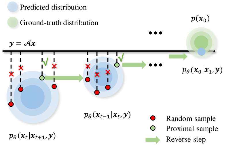
To tackle the challenges posed by random sampling, in this paper, we propose to extract multiple candidate samples from the predicted distribution, and select the most proximal one to our anticipated target. Our motivation comes from the following idea: considering $\mathbf{x}_{0}^{*}$ is an ideal but unknown solution for the image restoration problem, the sample taken from the predicted distribution $\mathbf{x}_{t-1}\sim p_{\mathbf{\theta}}(\mathbf{x}_{t-1}|\mathbf{x}_{t},\mathbf{y})$ should be close to posterior $q(\mathbf{x}_{t-1}|\mathbf{x}_{t},\mathbf{x}_{0}^{*})$, as it models the desired reverse process. The mathematical formulation of our selection process is given by:

$$\mathbf{x}_{t-1}= \operatorname*{arg\,min}_{\mathbf{x}_{t-1}^{i}}\|\mathbf{x}_{t-1}^{i}-\mathbf{x}_{t-1}^{*}\|_{2}^{2}$$ (9)

where $\mathbf{x}_{t-1}^{i}\sim p_{\mathbf{\theta}}(\mathbf{x}_{t-1}|\mathbf{x}_{t},\mathbf{y}),~{}i\in[0,n-1]$, $\mathbf{x}_{0}^{*}$ denotes the unknown solution for Eq. (5), and $\mathbf{x}_{t-1}^{*}$ is our proposed deterministic solution via DDIM (Song et al., 2021a) (see Appendix B for detailed derivation):

$$\mathbf{x}_{t-1}^{*}= \sqrt{\bar{\alpha}_{t-1}}{\mathbf{x}}_{0}^{*}+\sqrt{1-\bar{\alpha}_{t-1}}\cdot\frac{\mathbf{x}_{t}-\sqrt{\bar{\alpha}_{t}}\mathbf{x}_{0}^{*}}{\sqrt{1-\bar{\alpha}_{t}}}$$ (10)

$$= C_{1}\mathbf{x}_{t}+C_{2}\mathbf{x}_{0}^{*}.$$

where $C_{1}={\sqrt{1-\bar{\alpha}_{t-1}}}/{\sqrt{1-\bar{\alpha}_{t}}}$ and $C_{2}=\sqrt{\bar{\alpha}_{t-1}}-{\sqrt{\bar{\alpha}_{t}}\sqrt{1-\bar{\alpha}_{t-1}}}/{\sqrt{1-\bar{\alpha}_{t}}}$ are introduced for simplicity.

However, accessing $\mathbf{x}_{0}^{*}$ during inference is infeasible, rendering $\mathbf{x}_{t-1}^{*}$ also unknown. Now, one important contribution of this paper is to project Eq. (9) onto the measurement subspace. This is feasible as $\mathcal{A}\mathbf{x}_{t-1}^{*}$ can be approximated under the condition $\mathbf{y}\approx\mathcal{A}\mathbf{x}_{0}^{*}$.

$$\mathcal{A}\mathbf{x}_{t-1}^{*}\approx C_{1}\mathcal{A}\mathbf{x}_{t}+C_{2}\mathbf{y}.$$ (11)

Specifically, by projecting onto the measurement subspace, we choose $\mathbf{x}_{t-1}$ by the following:

$$\mathbf{x}_{t-1}=\operatorname*{arg\,min}_{\mathbf{x}_{t-1}^{i}}\|\mathcal{A}(\mathbf{x}_{t-1}^{i}-\mathbf{x}_{t-1}^{*})\|_{2}^{2}$$ (12)

Since $\mathbf{x}_{0}^{*}$ is expected to be more accurate than the denoised result $\hat{\mathbf{x}}_{0|t}$, the measurement $\mathbf{y}\approx\mathcal{A}\mathbf{x}_{0}^{*}$ can provide a stable and strong supervisory signal to correct the sampling result. Then by means of sample selection, we effectively control the result $\mathbf{x}_{t-1}$ within a more desirable region, even though we have no access to the $\mathbf{x}_{0}^{*}$.

The underlying motivation of our approach is depicted in Figure 3. Without changing the diffusion denoiser, our approach directs the sampling results toward a predefined target, mitigating the drawbacks induced by randomness. Moreover, the generative process remains stochastic, benefiting from the injected noise (Bao et al., 2021; Karras et al., 2022) since it corrects prediction errors and imprecise parameter settings from previous steps. Consequently, our method converges more rapidly and attains superior results.

As $\mathcal{A}$ is irreversible and complex in numerous scenarios, we propose to randomly sample $n$ candidates $\mathbf{x}_{t-1}^{i},i\in[0,n-1]$ from the predicted distribution $p_{\mathbf{\theta}}(\mathbf{x}_{t-1}|\mathbf{x}_{t},\mathbf{y})$, and choose the one with the minimal deviation from our anticipated values. Finally, Eq. (9) becomes:

$$\mathbf{z}_{t}= \operatorname*{arg\,min}_{\mathbf{z}_{t}^{i}}\|\mathcal{A}\left(\bm{\mu}_{\mathbf{\theta}}(\mathbf{x}_{t},t,\mathbf{y})+\sigma_{t}\mathbf{z}_{t}^{i}-C_{1}\mathbf{x}_{t}\right)-C_{2}\mathbf{y}\|_{2}^{2}$$ (13)

The process of sample selection is also denoted as noise selection, given by $\mathbf{x}_{t-1}^{i}=\bm{\mu}_{\mathbf{\theta}}(\mathbf{x}_{t},t,\mathbf{y})+\sigma_{t}\mathbf{z}_{t}^{i}$. We detail the full algorithm in Algorithm 2, and name our algorithm Diffusion Posterior Proximal Sampling (DPPS). The chosen $\mathbf{x}_{t-1}$ is referred to as the proximal sample due to the similarity to the proximal operator (Parikh & Boyd, 2014). An ablation study concerning the number of candidate samples $n$ is presented in Section 5.4.

Figure 3: Conceptual illustration of our DPPS. Our method extract multiple candidate samples from the predicted distribution and choose the one with the highest measurement consistency.

3.2 Aligned Initialization

When training, the diffusion model is trained with samples from $q(\mathbf{x}_{T}|\mathbf{x}_{0})$. However, diffusion-based restoration algorithm starts from the Gaussian distribution $\mathcal{N}(\mathbf{0},\mathbf{I})$. Recent studies have pointed out that initializition have a significant impact on the generated results (Singh et al., 2022; Cao et al., 2023; Ma et al., 2023), and the discrepancy between the two distributions account for a discretization error (Benton et al., 2023). In this paper, inspired by (Everaert et al., 2023), we simply initialize the sample in the same way as during training, making the best use of the available measurement

$$\mathbf{x}_{T}=\sqrt{\bar{\alpha}_{T}}\mathcal{A}^{T}\mathbf{y}+\sqrt{1-\bar{\alpha}_{T}}\bm{\epsilon}\quad\bm{\epsilon}\sim\mathcal{N}(\mathbf{0},\mathbf{I}).$$ (14)

where $\mathcal{A}^{T}$ means the transpose of operator. We argue this trick provides a modicum of information as a signal to the reverse model, as it realigns the distribution of initial latent with the training distribution (Everaert et al., 2023).

3.3 Discussion

Relevance to Existing Methods.  DPS (Chung et al., 2023a) proposes to estimate the intractable likelihood under Laplacian approximation, and adopts random sampling from the predicted distribution. However, the randomly chosen sample may not be well-coordinated with the measurement information. Another study MCG (Chung et al., 2022) iteratively applies projection onto the measurement subspace after the denoising step to ensure data consistency. However, the imposed projections lead to accumulated error due to measurement noise.

Our algorithm can be viewed as a special case of DPS, where we choose the sample that exhibits better measurement consistency. It absorbs the advantages of the robustness to noise from DPS and the faithful data consistency of MCG. Moreover, the better data consistency is achieved by injecting a guided adaption $\mathbf{z}_{t}$, which also helps correct the prediction errors in last generation steps (Karras et al., 2022; Jolicoeur-Martineau et al., 2021), leading to enhanced output quality.

Computational Efficiency.  Selecting the proximal sample introduces some extra computational overhead. In practice, the diffusion model conducts back-propagation only once, aligning with the mainstream approaches (Song et al., 2022; Chung et al., 2022, 2023a; Song et al., 2023c). The evaluations for Eq. (13) are considerably cheaper than gradient calculation, making the additional computational costs manageable. We show the computational resources for different settings in Section C.2.

Theoretical Analysis. 

Here, we provide some theoretical supports for our methodology. Despite our proposed proximal sampling being random, we can theoretically approach the desired point within an upper bound with mild assumptions. The proposition, detailed in Appendix B, proves that we can converge to our desired target $\mathbf{x}_{t-1}^{*}$, when the number of candidate samples is large enough. Furthermore, our method doesn’t require an exceptionally large number of candidates to achieve promising performance. This is because the variance of our method decreases when the proximal one is selected from any number of candidates.

Proposition 3.1.

For the random variable $\mathbf{z}\sim\mathcal{N}(\mathbf{0},\mathbf{I})$ and its objective function:

$$f(\mathbf{z})=\|\mathcal{A}(\bm{\mu}_{\mathbf{\theta}}(\mathbf{x}_{t},t,\mathbf{y})+\sigma_{t}\mathbf{z}-C_{1}\mathbf{x}_{t})-C_{2}\mathbf{y}\|^{2}_{2}.$$ (15)

The variance for $f(\mathbf{z})$ is denoted by $\text{Var}\left(f(\mathbf{z})\right)$. We have

$$\text{Var}_{\text{DPS}}\left(f(\mathbf{z})\right)>\text{Var}_{\text{MC}}\left(f(\mathbf{z})\right)>\text{Var}_{\text{Ours}}\left(f(\mathbf{z})\right).$$ (16)

Here, $\text{Var}_{\text{DPS}}\left(f(\mathbf{z})\right)$ is the variance of DPS (Chung et al., 2023a), $\text{Var}_{\text{MC}}\left(f(\mathbf{z})\right)$ is the variance of Monte Carlo sampling, and $\text{Var}_{\text{Ours}}\left(f(\mathbf{z})\right)$ is the variance of our proximal sampling method.

We provide a proof in Appendix B. In line with our theoretical analysis, empirical observations suggest that the proximal sample strategy demonstrates improved data consistency and reduced stochasticity, as evidenced by the experimental results.

Figure 4: Image restoration results with $\sigma_{y}=0.01$. Row 1: SR ($\times$4), Row 2: 80% inpainting, Row 3: Gaussian deblurring.

4 Related Work

To solve image restoration or image inverse problems with diffusion models, plenty of notable works (Dhariwal & Nichol, 2021; Kawar et al., 2022; Chung et al., 2023a; Song et al., 2023b) have been introduced. The first category of approaches (Saharia et al., 2021; Dhariwal & Nichol, 2021; Saharia et al., 2022) involves training conditional diffusion models or approximating the likelihood with synthetic image pairs as training data. However, these methods require specific training for each task and lack generalization across a wide range of inverse problems.

In contrast, the second category of approaches addresses inverse problems with unconditional diffusion models by guiding the reverse diffusion process (Song et al., 2022; Zhu et al., 2023). Several studies (Song et al., 2023b; Chung et al., 2023a; Song et al., 2023c) concentrate on estimating the time-dependent likelihood $p_{t}(\mathbf{y}|\mathbf{x}_{t})$ for posterior sampling. Among them, Song et al. (2023c) enhances the likelihood approximation with a Monte-Carlo estimate. Ma et al. (2023) tackles image super-resolution by selecting the best starting point from multiple choices. Recently, latent diffusion models have also seen advancements (Rombach et al., 2022; Vahdat et al., 2021) and have been widely adopted in various image inverse problem scenarios (Rout et al., 2023b; He et al., 2023; Song et al., 2023a; Chung et al., 2023b; Rout et al., 2023a).

5 Experiments

5.1 Setup

Dataset, Model.  To showcase the effectiveness of the proposed methods, we conducted experiments on two standard datasets, namely FFHQ 256$\times$256 (Karras et al., 2019) and ImageNet 256$\times$256 (Russakovsky et al., 2015). The evaluation encompasses the first 1k images in the validation set of each dataset. The diffusion models pre-trained on ImageNet and FFHQ are sourced from Dhariwal & Nichol (2021) and Chung et al. (2023a), respectively. For comprehensive comparisons, we include state-of-the-art diffusion-based image restoration solvers, including the Plug-and-play alternating direction method of multipliers (PnP-ADMM) (Chan et al., 2016), Score-SDE (Song et al., 2022), Denoising Diffusion Restoration Models (DDRM) (Kawar et al., 2022), Manifold Constrained Gradient (MCG) (Chung et al., 2022), DPS (Chung et al., 2023a), and DiffPIR (Zhu et al., 2023). To ensure fair comparisons, we utilized the same pre-trained diffusion models for all diffusion-based methods. Additional details, including hyper-parameters and metrics, are provided in Appendix D. All experiments were executed with a fixed random seed unless explicitly stated.

Table 1: Quantitative evaluation of image restoration tasks on FFHQ 256$\times$256-1k and ImageNet 256$\times$256-1k with $\sigma_{y}=0.01$. Bold: best, underline: second best.

	Inpaint (random)				Deblur (Gaussian)				Deblur (motion)				SR ($\times$ 4)
Method	PSNR $\uparrow$	SSIM $\uparrow$	LPIPS $\downarrow$	FID $\downarrow$	PSNR $\uparrow$	SSIM $\uparrow$	LPIPS $\downarrow$	FID $\downarrow$	PSNR $\uparrow$	SSIM $\uparrow$	LPIPS $\downarrow$	FID $\downarrow$	PSNR $\uparrow$	SSIM $\uparrow$	LPIPS $\downarrow$	FID $\downarrow$
FFHQ
PnP-ADMM (Chan et al., 2016)	27.32	0.743	0.349	63.19	25.97	0.744	0.260	94.50	25.86	0.724	0.278	59.06	26.94	0.792	0.292	90.11
Score-SDE (Song et al., 2021b)	21.91	0.610	0.371	58.19	18.37	0.256	0.629	169.68	15.79	0.246	0.635	176.73	24.10	0.705	0.363	75.50
MCG (Chung & Ye, 2022)	24.59	0.711	0.265	29.31	19.67	0.549	0.497	85.85	18.00	0.513	0.604	91.73	24.02	0.698	0.321	52.88
DDRM (Kawar et al., 2022)	21.85	0.643	0.378	78.40	26.38	0.743	0.298	62.72	-	-	-	-	27.31	0.806	0.248	52.49
DPS (Chung et al., 2023a)	27.29	0.816	0.182	23.11	26.04	0.742	0.228	30.52	25.24	0.726	0.261	33.47	26.55	0.763	0.237	34.50
DiffPIR (Zhu et al., 2023)	27.96	0.820	0.210	30.38	25.38	0.700	0.276	32.00	22.74	0.654	0.331	83.42	24.74	0.710	0.273	33.03
Ours	27.47	0.834	0.168	18.98	26.40	0.752	0.220	29.29	26.88	0.783	0.214	28.95	26.93	0.778	0.203	26.30
ImageNet
PnP-ADMM (Chan et al., 2016)	25.14	0.685	0.405	66.54	21.97	0.584	0.419	63.15	21.86	0.676	0.408	61.46	23.95	0.710	0.346	71.41
Score-SDE(Song et al., 2021b)	16.25	0.241	0.653	102.56	21.31	0.594	0.467	82.54	13.56	0.418	0.661	89.62	17.69	0.316	0.624	96.67
MCG (Chung & Ye, 2022)	23.21	0.661	0.324	44.09	12.31	0.405	0.647	109.45	18.32	0.463	0.633	99.26	17.08	0.292	0.538	85.91
DDRM (Kawar et al., 2022)	19.34	0.460	0.555	147.00	23.67	0.635	0.401	66.99	-	-	-	-	25.49	0.729	0.319	54.77
DPS (Chung et al., 2023a)	25.65	0.780	0.240	29.04	19.65	0.487	0.422	65.35	18.79	0.465	0.458	77.29	23.88	0.667	0.335	42.83
DiffPIR (Zhu et al., 2023)	25.85	0.797	0.235	33.16	22.03	0.569	0.395	54.71	19.86	0.534	0.433	79.23	24.78	0.712	0.302	39.25
Ours	24.97	0.758	0.217	24.90	22.70	0.609	0.364	51.21	21.65	0.592	0.375	51.35	24.79	0.712	0.276	33.75

Degradation Operator.  The degradation operators are defined as follows: (i) For inpainting, 80% of the pixels (all RGB channels) in the image are masked. (ii) For Gaussian blur, a blur kernel of size $61\times 61$ with a standard deviation of $3.0$ is employed. (iii) For motion blur, the kernel, following the procedure outlined in Chung et al. (2022), has a size of $61\times 61$ and an intensity value of $0.5$. (iv) For SR $\times~{}4$, the operator involves $4\times$ bicubic down-sampling. Additive Gaussian noise with a variance of $\sigma_{y}=0.01$ is applied for all degradation processes.

5.2 Results

Main Results.  We present the statistic results of the general image restoration tasks on both FFHQ and ImageNet datasets, as detailed in Table 1. To the dataset with homogeneous scenarios, i.e., FFHQ, our proposed method demonstrates impressive results across all metrics, establishing its superiority over existing state-of-the-art methods. When dealing with more varied images within the ImageNet dataset, our approach exhibits substantial outperformance against all baseline methods in terms of FID and LPIPS, while maintaining comparable levels in PSNR.

Figure 7: Visual results on SR ($\times$4) task to demonstrate the efficacy of our proposed method and to explore the impact of $n$. More results are presented in Appendix F.

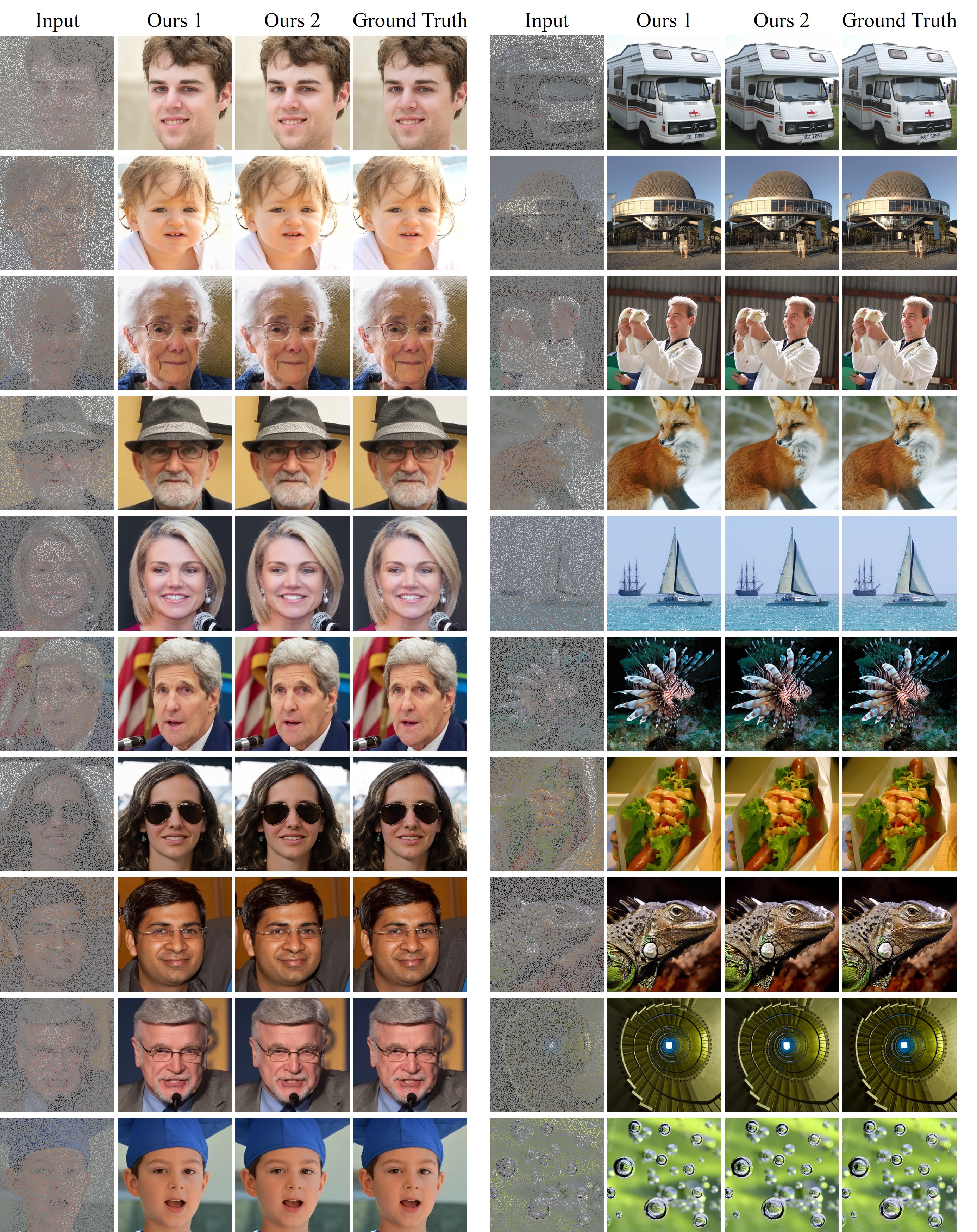
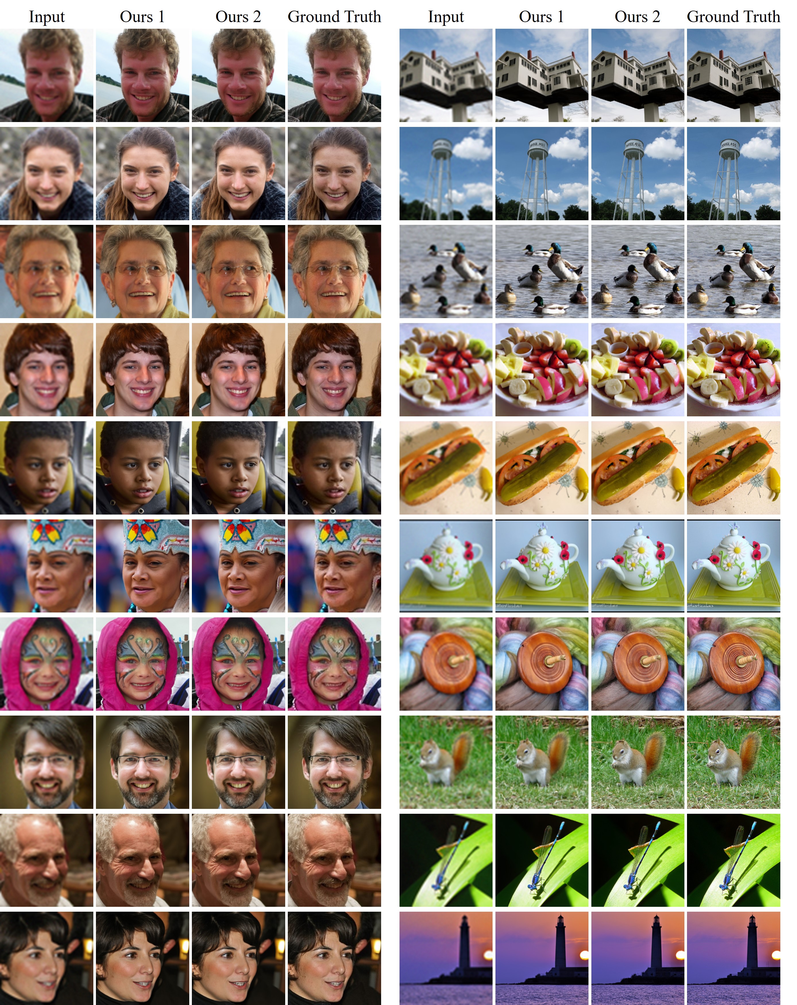
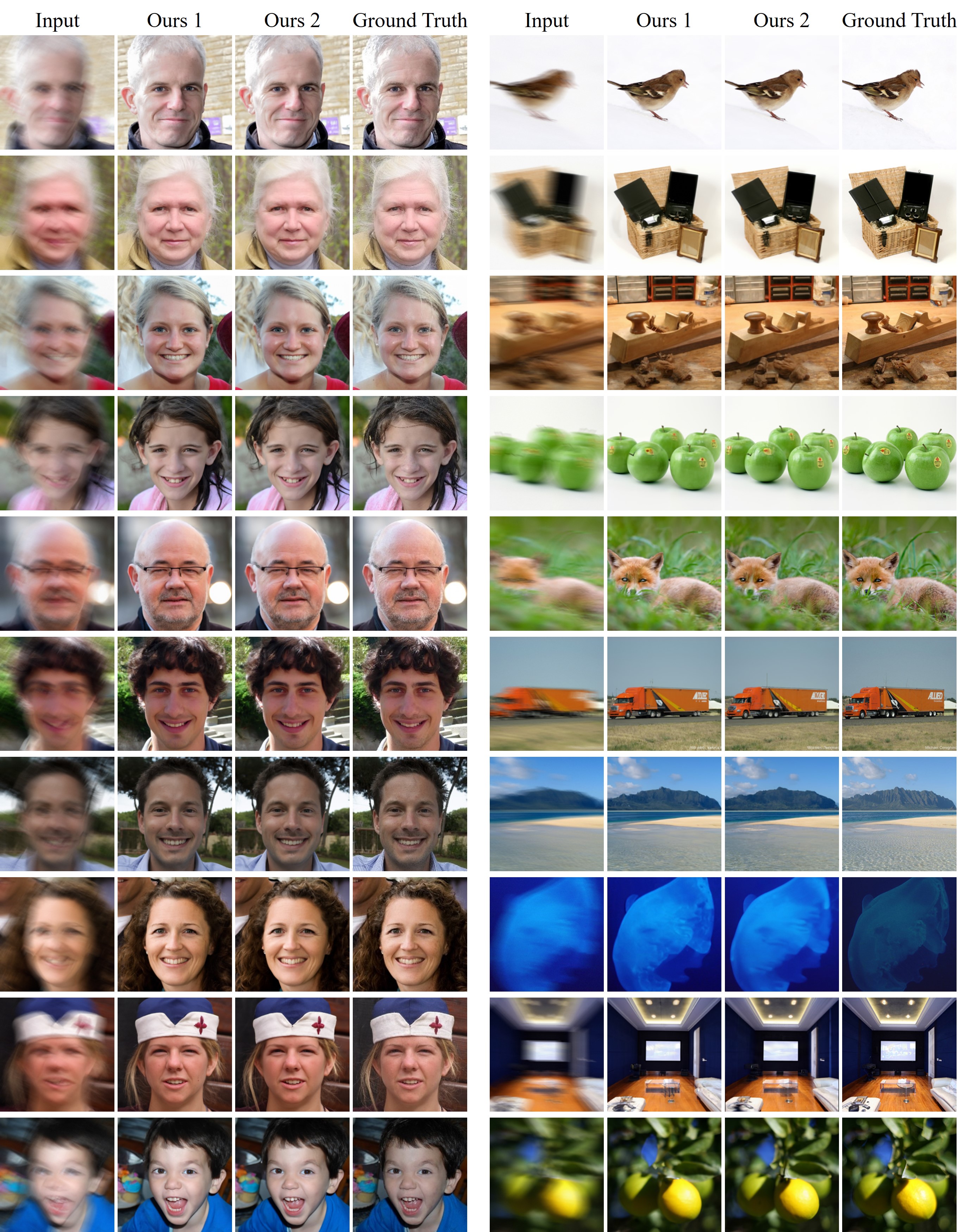
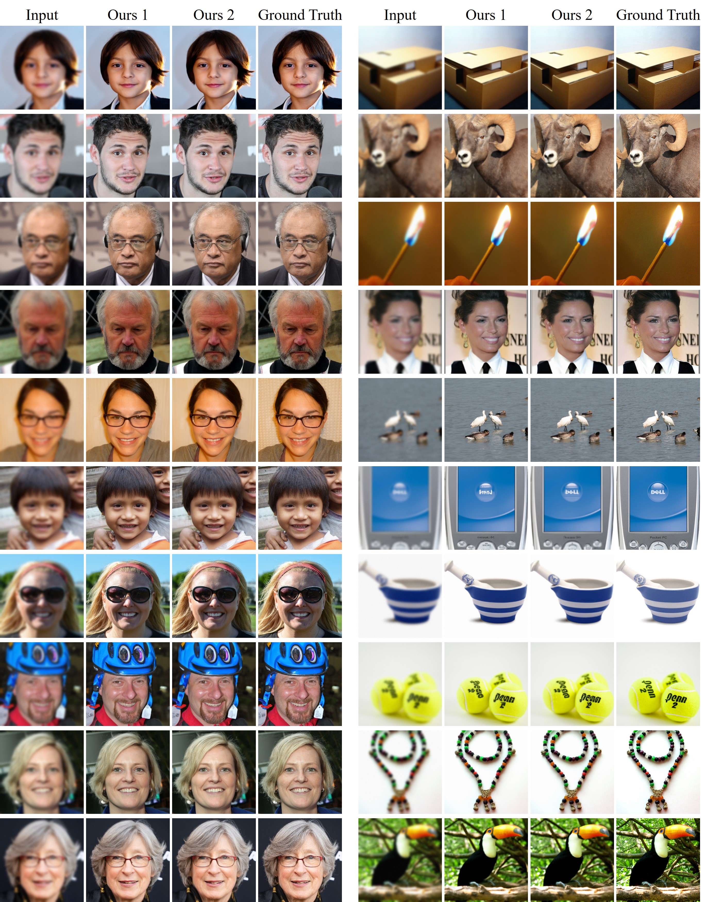
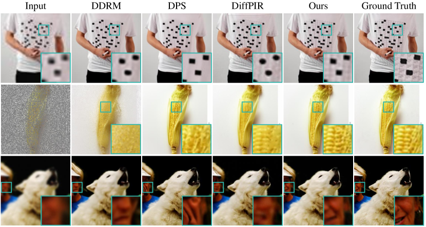
The visual results for inpainting, SR, and Gaussian deblurring are shown in Figure 4, showcasing the evident superiority of our proposed method. While DDRM attains commendable distortion results with fewer Neural Function Evaluations (NFEs), it faces limitations in reliably restoration results for image inpainting tasks characterized by a very low rank of the measurement. DiffPIR achieves satisfactory results in various scenarios; however, its performance is tied to the analytical solution for the data consistency term and exhibits sensitivity to measurement noise. DPS differs from our approach in that it introduces random noise at each generation step, leading to over-smoothed and unstable restoration results, as depicted in Figure 4 (row 3). Conversely, our proposed method circumvents such drawbacks. The generative process is stabilized by directing the sample to a predefined target, yielding realistic and detailed restoration outcomes. It is noteworthy that the generated results from our method exhibit minimal variation with different seeds (refer to Appendix F for additional visual results), aligning with the intended design of identity preserving.

5.3 The Effect of Proximal Sampling

Faster Convergence. To investigate the impact of our proximal sampling on the generated results, we conducted further experimental analyses using the first 150 images from the FFHQ validation set. In addition to the native DPS, we incorporated the results of DPS with DDIM (Song et al., 2021a) deterministic sampling, denoted as DPS_DDIM, which mitigates the effects of randomness. Results for (a) mean of $\|\mathbf{y}-\mathcal{A}\hat{\mathbf{x}}_{0|t}\|_{2}^{2}$, (b) average LPIPS of $\hat{\mathbf{x}}_{0|t}$, and (c) average PSNR of $\hat{\mathbf{x}}_{0|t}$ over timesteps are reported in LABEL:fig:Convergence_speed. It is evident that our method facilitates a more stable optimization process, yielding markedly superior results compared to DPS and DPS_DDIM within the same period. This observation also supports the claim that the measurement can provide reliable supervisory signals for the sampling result.

More Robust to Hyper-parameter.  We anticipate that our proposed proximal sampling serves as an adaptive correction for prediction errors resulting from imprecise parameter settings. To substantiate this claim, we conducted experiments with different $\lambda_{t}$, comparing the results of our proximal sampling with those obtained through random sampling.

Figure 8: FID comparison between random sampling and proximal sampling with different values of $\lambda_{t}$.

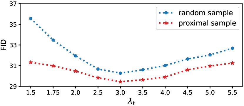
As illustrated in Figure 8, our method consistently outperforms random sampling across different parameter settings. Notably, the performance of the random sampling method exhibits fluctuations with changes in parameters. In contrast, our method demonstrates stability over a range of parameter configurations, thereby validating the assertion.

5.4 Ablation Study

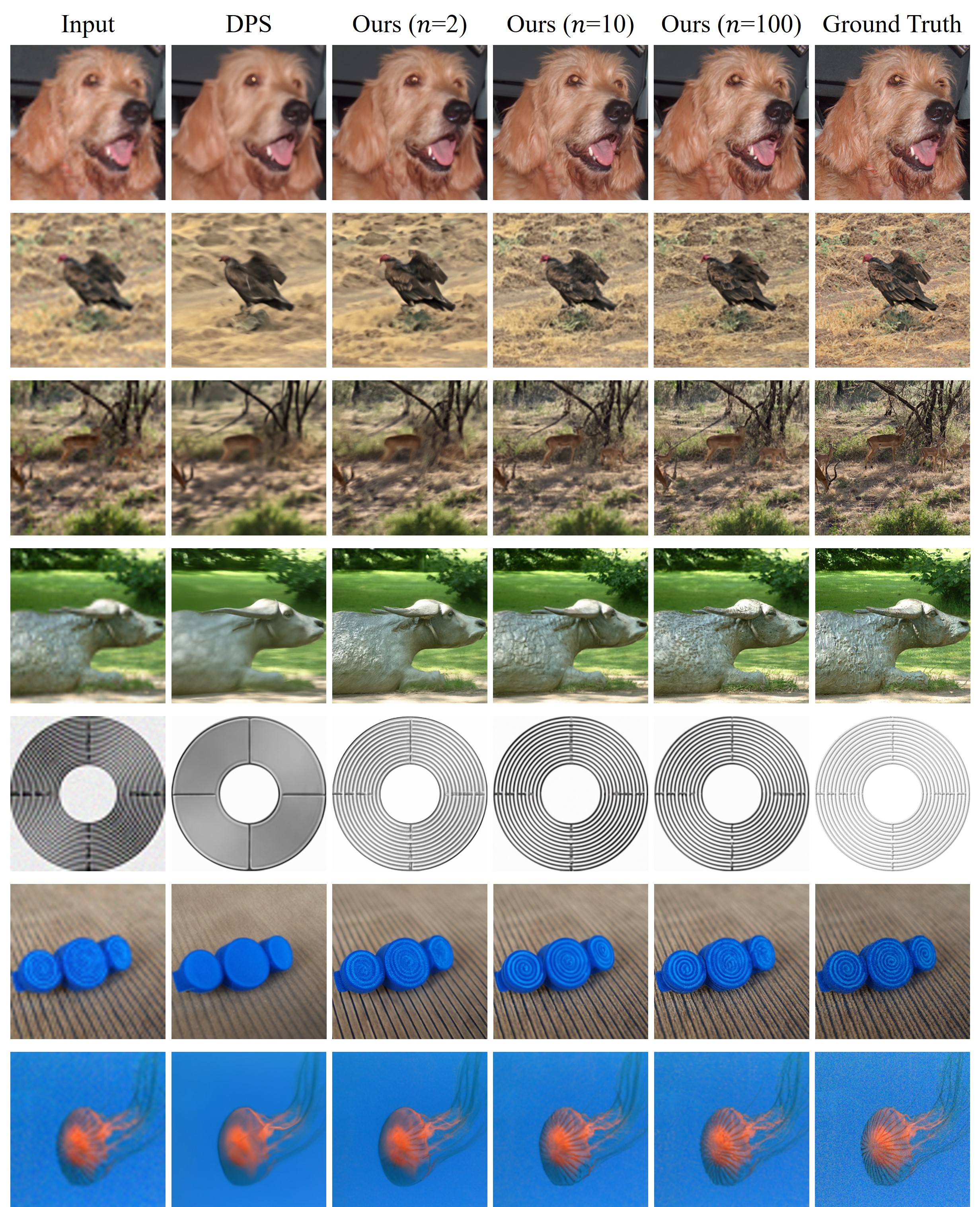
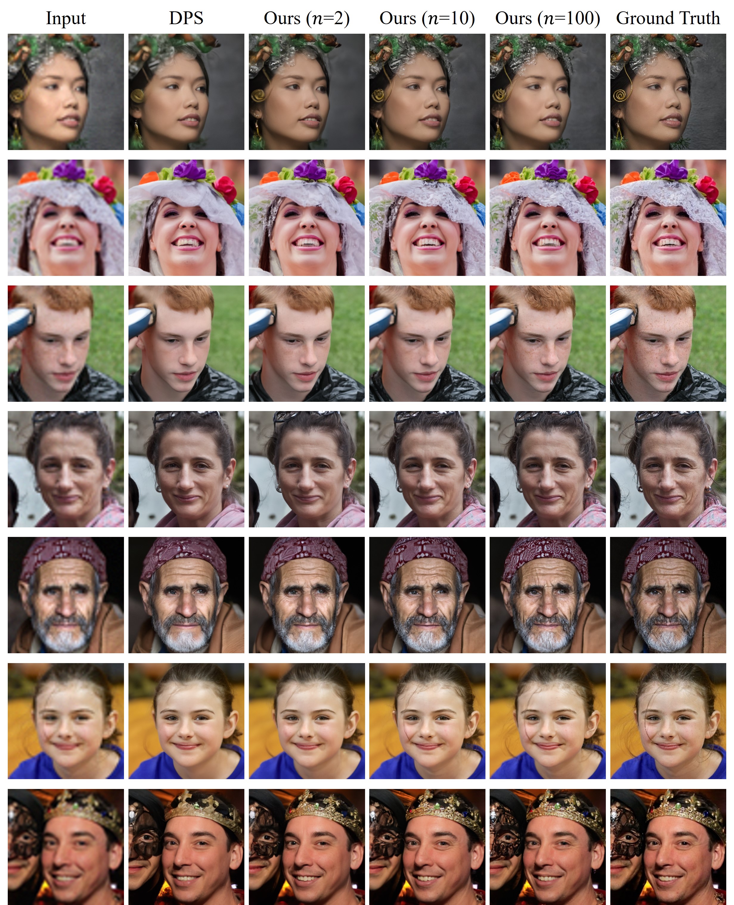
The Number of Candidate Samples.  The number of samples, denoted as $n$, stands out as a pivotal parameter of the proposed methodology. The ablation studies relating to $n$ are shown in Table 2 and Figure 7. Figure 7 illustrates a noticeable enhancement in output quality and details with increasing $n$. This observation is reinforced by Table 2, where both the LPIPS and FID metrics exhibit a notable decrease as $n$ increases. The augmented number of candidate samples corresponds to a higher likelihood of proximity to the intended target, thereby providing enhanced supervision for the generative process. This reaffirms the reliability and applicability of the proposed methodology. It is noteworthy that the improvement becomes relatively marginal when $n$ exceeds 20 and may even result in a decrease in PSNR. We posit that measurement noise ($\mathbf{n}$ in Eq. (5)) influences the precision of our approximation. Moreover, sample selection is conducted within the range space, introducing a certain degree of misalignment with the null space. Consequently, we set $n=20$ in our experiments to strike a balance between perceptual metrics, distortion metrics, and speed.

Table 2: Ablation studies on the number of candidate samples.

	FFHQ			ImageNet
Method	PSNR$\uparrow$	LPIPS$\downarrow$	FID$\downarrow$	PSNR$\uparrow$	LPIPS$\downarrow$	FID$\downarrow$
$n$=1	26.44	0.235	34.91	23.95	0.336	43.54
$n$=2	26.64	0.221	31.19	24.42	0.328	40.63
$n$=10	26.77	0.207	27.60	24.64	0.282	34.05
$n$=20∗	26.93	0.203	26.30	24.79	0.276	33.75
$n$=100	26.83	0.201	25.79	24.72	0.268	32.91

Noise Level.  The precision of the approximation is impacted by the level of measurement noise $\mathbf{n}$. We explore the effects of different noise levels on the proposed method compared with random sampling. The results presented in Table 3 reveal that (i) both methods experience a decline in performance as the noise level increases, and our approach consistently outperforms random sampling in all settings. (ii) For inpainting, both methods experience considerable degradations as the noise level increases, demonstrating sensitivity to the noise levels. (iii) For SR, notable performance degradation is observed in our method as the noise level increases, while the method adopting random sampling demonstrates greater robustness in this regard.

Design Components.  The proposed method consists of two design components: aligned initialization and proximal sample selection. To evaluate the impact of these components on overall performance, we conducted ablation experiments on the inpainting task. The results, as presented in Table 4, highlight that the proximal sample selection is a pivotal component, significantly contributing to performance improvements. While our aligned initialization method contributes moderately to the enhancement, more analyses can be found in Section C.1.

Table 3: Comparison of the impact of different noise levels.

		Inpainting			SR$\times$4
$\sigma_{y}$	Method	PSNR$\uparrow$	LPIPS$\downarrow$	FID$\downarrow$	PSNR$\uparrow$	LPIPS$\downarrow$	FID$\downarrow$
	Random	27.69	0.173	21.11	26.61	0.235	34.55
0.0	Ours	27.24	0.158	17.73	26.87	0.199	26.19
	Random	27.29	0.182	23.11	26.55	0.237	34.50
0.01	Ours	27.47	0.168	18.98	26.93	0.203	26.30
	Random	26.68	0.228	30.63	25.89	0.257	34.59
0.05	Ours	26.51	0.208	24.62	26.07	0.245	30.67

6 Conclusion

In this paper, we introduce a novel approach to mitigate problems caused by misaligned random sampling in diffusion-based image restoration methods. Specifically, our approach advocates selecting the proximal sample that is more consistent with the measurement in the predicted distribution at each generative step. In addition, we propose a realignment of the inference initialization involving measurement information to better align with expected generations. Experimental results validate a substantial performance improvement compared to SOTA methods. Our method innovatively takes advantage of stochastic sampling in the diffusion generative process to enhance the generation quality, offering new insights for future work.

7 Impact Statements

This paper presents work whose goal is to advance the field of Machine Learning. There are many potential societal consequences of our work, none which we feel must be specifically highlighted here.

Appendix A Score-based Diffusion Models

Here, we review the continues form of diffusion model introduced for completeness. The forward process of diffusion can be formulated by an Itô SDE:

$$\mathrm{d}\mathbf{x}=\mathbf{f}(\mathbf{x},t)\mathrm{d}t+g(t)\mathrm{d}\mathbf{w},$$ (17)

where $\mathbf{f}(\cdot,t):{\mathbb{R}}^{d}\mapsto{\mathbb{R}}^{d}$ is a drift coefficient function, ${g}(t)\in{\mathbb{R}}$ is a scalar function known as the diffusion coefficient, and $\mathbf{w}\in{\mathbb{R}}^{d}$ is the standard Wiener process. The forward process of DDPM can be viewed as variance-preserving (VP) SDE (Song et al., 2021b) as the total variance is preserved.

Correspondingly, the reversed generative (i.e., denoising) process is given by the reverse-time SDE:

$$\mathrm{d}\mathbf{x}=[\mathbf{f}(\mathbf{x},t)-g^{2}(t)\nabla_{\mathbf{x}_{t}}\log p_{t}(\mathbf{x}_{t})]\mathrm{d}t+g(t)\mathrm{d}\mathbf{\bar{w}},$$ (18)

where $\mathrm{d}\mathbf{\bar{w}}$ denotes the standard Wiener process running backward in time and $p_{t}(\mathbf{x}_{t})$ denotes the marginal probability density w.r.t. $\mathbf{x}$ at time $t$. In practice, a time-dependent network $\mathbf{s}_{\mathbf{\theta}}(\mathbf{x}_{t},t)$ parameterized by $\mathbf{\theta}$ is trained to approximate the (Stein) score function $\nabla_{\mathbf{x}_{t}}\log p_{t}(\mathbf{x}_{t})$ with score-matching method (Vincent, 2011):

$$\min_{\mathbf{\theta}}\mathbb{E}_{t,\mathbf{x}_{0},\mathbf{x}_{t}}\big{[}\|\mathbf{s}_{\mathbf{\theta}}(\mathbf{x}_{t},t)-\nabla_{\mathbf{x}_{t}}\log p(\mathbf{x}_{t}|\mathbf{x}_{0})\|_{2}^{2}\big{]},$$ (19)

where $t$ is uniformly sampled from $[0,T]$, $\mathbf{x}_{0}\sim q_{data}(\mathbf{x})$ and $\mathbf{x}_{t}\sim q(\mathbf{x}_{t}|\mathbf{x}_{0})$. Once we have aceess to the well-trained $\mathbf{s}_{\mathbf{\theta}}(\mathbf{x}_{t},t)$, an clean sample can be derived by simulating the generative reverse-time SDE (18) using numerical solvers (e.g. Euler-Maruyama).

Appendix B Additional Details

B.1 Derivation for $\mathbf{x}_{t-1}^{*}$

We show the detailed derivation and explanation for the $\mathbf{x}_{t-1}^{*}$ in Equation 9. Our motivation was to give the stochastic sampling process a supervision at inference, trying to make the sampled $\mathbf{x}_{t-1}$ in the vicinity of the theoretically derived solution. Recall the inference distributions defined in (Song et al., 2021a):

$$q(\mathbf{x}_{t-1}|\mathbf{x}_{t},\mathbf{x}_{0}^{*})={\cal N}(\sqrt{\bar{\alpha}_{t-1}}\mathbf{x}_{0}^{*}+\sqrt{1-\bar{\alpha}_{t-1}-\sigma_{t}^{2}}\cdot\frac{\mathbf{x}_{t}-\sqrt{\bar{\alpha}_{t}}\mathbf{x}_{0}^{*}}{\sqrt{1-\bar{\alpha}_{t}}},\sigma_{t}^{2}\mathbf{I}).$$ (20)

By setting $\sigma_{t}=0$, we get our deterministic denoised estimate $\mathbf{x}_{t-1}^{*}$

$$\mathbf{x}_{t-1}^{*}= \sqrt{\bar{\alpha}_{t-1}}{\mathbf{x}}_{0}^{*}+\sqrt{1-\bar{\alpha}_{t-1}}\cdot\frac{\mathbf{x}_{t}-\sqrt{\bar{\alpha}_{t}}\mathbf{x}_{0}^{*}}{\sqrt{1-\bar{\alpha}_{t}}}$$ (21)

$$= \frac{\sqrt{1-\bar{\alpha}_{t-1}}}{\sqrt{1-\bar{\alpha}_{t}}}\mathbf{x}_{t}+(\sqrt{\bar{\alpha}_{t-1}}-\frac{\sqrt{\bar{\alpha}_{t}}\cdot\sqrt{1-\bar{\alpha}_{t-1}}}{\sqrt{1-\bar{\alpha}_{t}}})\mathbf{x}_{0}^{*}.$$

Then we have the approximation for $\mathcal{A}\mathbf{x}_{t-1}^{*}$:

$$\mathcal{A}\mathbf{x}_{t-1}^{*}=\frac{\sqrt{1-\bar{\alpha}_{t-1}}}{\sqrt{1-\bar{\alpha}_{t}}}\mathcal{A}\mathbf{x}_{t}+(\sqrt{\bar{\alpha}_{t-1}}-\frac{\sqrt{\bar{\alpha}_{t}}\cdot\sqrt{1-\bar{\alpha}_{t-1}}}{\sqrt{1-\bar{\alpha}_{t}}})\mathcal{A}\mathbf{x}_{0}^{*}.$$ (22)

By applying $\mathbf{y}=\mathcal{A}\mathbf{x}_{0}^{*}+\mathbf{n}$,

$$\mathcal{A}\mathbf{x}_{t-1}^{*}= \frac{\sqrt{1-\bar{\alpha}_{t-1}}}{\sqrt{1-\bar{\alpha}_{t}}}\mathcal{A}\mathbf{x}_{t}+(\sqrt{\bar{\alpha}_{t-1}}-\frac{\sqrt{\bar{\alpha}_{t}}\cdot\sqrt{1-\bar{\alpha}_{t-1}}}{\sqrt{1-\bar{\alpha}_{t}}})(\mathbf{y}-\mathbf{n})$$ (23)

$$\approx \frac{\sqrt{1-\bar{\alpha}_{t-1}}}{\sqrt{1-\bar{\alpha}_{t}}}\mathcal{A}\mathbf{x}_{t}+(\sqrt{\bar{\alpha}_{t-1}}-\frac{\sqrt{\bar{\alpha}_{t}}\cdot\sqrt{1-\bar{\alpha}_{t-1}}}{\sqrt{1-\bar{\alpha}_{t}}})\mathbf{y}$$

The approximation of last step holds when $\sigma_{y}$ is assumed in a small range as $\mathbf{n}\sim\mathcal{N}(\mathbf{0},\mathbf{\sigma_{y}}\mathbf{I})$.

Proposition B.1.

Assume that $\|\mathbf{y}\|_{2}\leq Y,\|\mathbf{x}_{0}^{*}\|_{2}\leq X,\|\mathbf{x}_{t-1}^{\prime}\|_{2}\leq X,\|\bm{\mu}_{\theta}(\mathbf{x}_{t},t,\mathbf{y})\|_{2}\leq E$ are bounded and continuous, there exists a upper bound for $\|\mathcal{A}\left(\mathbf{x}_{t-1}^{i}-\mathbf{x}^{*}_{t-1}\right)\|_{2}^{2}$ which is:

$$\|\mathcal{A}\left(\mathbf{x}_{t-1}^{i}-\mathbf{x}^{*}_{t-1}\right)\|_{2}^{2}\leq\left(\mathcal{A}E-\mathcal{A}X+\mathcal{A}\sigma_{t}\right)^{2}.$$ (24)

It is proven that some linear (i.e. super-resolution and inpainting) operators $\mathcal{A}$ can be modeled as matrices (Chung et al., 2023a) which are bounded and linear. And for $\sigma_{t}$, it is usually set to a small value which is also bounded. Thus, we can conclude that the above upper bound holds.

Proof.

$$\|\mathcal{A}\left(\mathbf{x}_{t-1}^{i}-\mathbf{x}^{*}_{t-1}\right)\|_{2}^{2} =\|\mathcal{A}\mathbf{x}_{t-1}^{i}-\mathcal{A}\mathbf{x}^{*}_{t-1}\|_{2}^{2}$$ (25)

$$\overset{(\text{a})}{\approx}\|\mathcal{A}\left(\bm{\mu}_{\theta}(\mathbf{x}_{t},t,\mathbf{y})+\sigma_{t}\mathbf{z}^{i}_{t}\right)-\left(\sqrt{\bar{\alpha}_{t-1}}\mathbf{y}+\sqrt{1-\bar{\alpha}_{t-1}}\cdot\frac{\mathcal{A}\mathbf{x}_{t}-\sqrt{\bar{\alpha}_{t}}\mathbf{y}}{\sqrt{1-\bar{\alpha}_{t}}}\right)\|_{2}^{2},$$ (26)

where $\mathbf{z}^{i}_{t}\sim\mathcal{N}(\mathbf{0},\mathbf{I})$ and the $\overset{(\text{a})}{\approx}$ is from Eq. (11). Here, we apply trigonometric inequalities to the above equation, we have:

$$\|\mathcal{A}\left(\mathbf{x}_{t-1}^{i}-\mathbf{x}^{*}_{t-1}\right)\|_{2}^{2} \overset{(\text{a})}{\approx}\|\mathcal{A}\left(\bm{\mu}_{\theta}(\mathbf{x}_{t},t,\mathbf{y})+\sigma_{t}\mathbf{z}^{i}_{t}\right)-\left(\sqrt{\bar{\alpha}_{t-1}}\mathbf{y}+\sqrt{1-\bar{\alpha}_{t-1}}\cdot\frac{\mathcal{A}\mathbf{x}_{t}-\sqrt{\bar{\alpha}_{t}}\mathbf{y}}{\sqrt{1-\bar{\alpha}_{t}}}\right)\|_{2}^{2}$$ (27)

$$\approx\|\left(\mathcal{A}\bm{\mu}_{\theta}(\mathbf{x}_{t},t,\mathbf{y})-\sqrt{\bar{\alpha}_{t-1}}\mathbf{y}\right)+\left(\sigma_{t}\mathcal{A}\mathbf{z}_{t}^{i}-\sqrt{1-\bar{\alpha}_{t-1}}\cdot\frac{\mathcal{A}\mathbf{x}_{t}-\sqrt{\bar{\alpha}_{t}}\mathbf{y}}{\sqrt{1-\bar{\alpha}_{t}}}\right)\|_{2}^{2}$$ (28)

$$\approx\left(\|\mathcal{A}\bm{\mu}_{\theta}(\mathbf{x}_{t},t,\mathbf{y})-\sqrt{\bar{\alpha}_{t-1}}\mathbf{y}\|_{2}+\|\sigma_{t}\mathcal{A}\mathbf{z}_{t}^{i}-\sqrt{1-\bar{\alpha}_{t-1}}\cdot\frac{\mathcal{A}\mathbf{x}_{t}-\sqrt{\bar{\alpha}_{t}}\mathbf{y}}{\sqrt{1-\bar{\alpha}_{t}}}\|_{2}\right)^{2}.$$ (29)

Since $\|\bm{\mu}_{\theta}(\mathbf{x}_{t},t,\mathbf{y})\|_{2}\leq E$, $\|\bar{\alpha}_{t}\|_{2}\leq A$, $\|\bar{\alpha}_{t}\|_{2}\leq A$, $\|\bar{\alpha}_{t-1}\|_{2}\leq A,$, and $\|\mathbf{y}\|_{2}\leq Y$, we have the upper bound for $\|\mathcal{A}\bm{\mu}_{\theta}(\mathbf{x}_{t},t,\mathbf{y})-\sqrt{\bar{\alpha}_{t-1}}\mathbf{y}\|_{2}$, and thus $\|\mathcal{A}\bm{\mu}_{\theta}(\mathbf{x}_{t},t,\mathbf{y})-\sqrt{\bar{\alpha}_{t-1}}\mathbf{y}\|_{2}\leq\mathcal{A}E-\sqrt{A}Y$. Similarly, we have the upper bound for $\|\sqrt{1-\bar{\alpha}_{t-1}}\cdot\frac{\mathcal{A}\mathbf{x}_{t}-\sqrt{\bar{\alpha}_{t}}\mathbf{y}}{\sqrt{1-\bar{\alpha}_{t}}}\|_{2}$, which is $\|\sqrt{1-\bar{\alpha}_{t-1}}\cdot\frac{\mathcal{A}\mathbf{x}_{t}-\sqrt{\bar{\alpha}_{t}}\mathbf{y}}{\sqrt{1-\bar{\alpha}_{t}}}\|_{2}\leq\mathcal{A}X-\sqrt{A}Y$. Therefore, we have:

$$\|\mathcal{A}\left(\mathbf{x}_{t-1}^{i}-\mathbf{x}^{*}_{t-1}\right)\|_{2}^{2} \overset{(\text{a})}{\approx}\|\mathcal{A}\left(\bm{\mu}_{\theta}(\mathbf{x}_{t},t,\mathbf{y})+\sigma_{t}\mathbf{z}^{i}_{t}\right)-\left(\sqrt{\bar{\alpha}_{t-1}}\mathbf{y}+\sqrt{1-\bar{\alpha}_{t-1}}\cdot\frac{\mathcal{A}\mathbf{x}_{t}-\sqrt{\bar{\alpha}_{t}}\mathbf{y}}{\sqrt{1-\bar{\alpha}_{t}}}\right)\|_{2}^{2}$$ (30)

$$\leq\left(\mathcal{A}E-\mathcal{A}X+\mathcal{A}\sigma_{t}\right)^{2}.$$ (31)

Chung et al. (2023a) has shown that some linear operations $\mathcal{A}$ (such as super-resolution and inpainting) can be represented as matrices that are linear and bounded. Moreover, $\sigma_{t}$ is typically chosen to be a small and finite number. Therefore, we can affirm that the upper bound in the previous equation is valid. ∎

Proposition B.2.

For the random variable $\mathbf{z}\sim\mathcal{N}(\mathbf{0},\mathbf{I})$ and its objective function:

$$f(\mathbf{z})=\|\mathcal{A}(\bm{\mu}_{\mathbf{\theta}}(\mathbf{x}_{t},t,\mathbf{y})+\sigma_{t}\mathbf{z}-C_{1}\mathbf{x}_{t})-C_{2}\mathbf{y}\|^{2}_{2},$$ (32)

where $C_{1}={\sqrt{1-\bar{\alpha}_{t-1}}}/{\sqrt{1-\bar{\alpha}_{t}}}$ and $C_{2}=\sqrt{\bar{\alpha}_{t-1}}-{\sqrt{\bar{\alpha}_{t}}\sqrt{1-\bar{\alpha}_{t-1}}}/{\sqrt{1-\bar{\alpha}_{t}}}$. Thus, with $M$ trials, each consisting of $N$ samples, we have the variance for $f(\mathbf{z})$, which is $\text{Var}\left(f(\mathbf{z})\right)$. We have

$$\text{Var}_{\text{DPS}}\left(f(\mathbf{z})\right)>\text{Var}_{\text{MC}}\left(f(\mathbf{z})\right)>\text{Var}_{\text{Ours}}\left(f(\mathbf{z})\right),$$ (33)

here, $\text{Var}_{\text{DPS}}\left(f(\mathbf{z})\right)$ is the variance of DPS (Chung et al., 2023a), $\text{Var}_{\text{MC}}\left(f(\mathbf{z})\right)$ is the variance of Monte Carlo sampling, and $\text{Var}_{\text{Ours}}\left(f(\mathbf{z})\right)$ is the variance of our proximal sampling method.

Proof.

For each trial, we only take one sample $\mathbf{z}_{1}$ from the distribution, and compute $f(\mathbf{z}_{1})$. Thus, for DPS, the estimation of a single sample is $\hat{\mu}_{\text{single}}=f(\mathbf{z}_{1})$, and the variance of the estimation is $\text{Var}\left(f(\mathbf{z})\right)$.

For Monte Carlo sampling, we draw $N$ independently and identically distributed samples $\mathbf{z}_{1},\mathbf{z}_{2},\dots,\mathbf{z}_{N}$, and compute the function $f(\mathbf{z}_{i})$ for each sample. Finally, we can get the estimation of a single trial as:

$$\hat{\mu}_{\text{MC}}=\frac{1}{N}\sum^{N}_{i=1}f(\mathbf{z}_{i}).$$ (34)

By the central limit theorem, when $N$ is large enough, the variance of $\hat{\mu}_{\text{MC}}$ is $\frac{\text{Var}\left(f(\mathbf{z})\right)}{N}$.

For our proximal sampling method, similar to Monte Carlo sampling, we also draw $N$ independently and identically distributed samples $\mathbf{z}_{1},\mathbf{z}_{2},\dots,\mathbf{z}_{N}$ for each trial, and compute the function $f(\mathbf{z}_{i})$ for each sample. However, we only get the estimation from the sample with the lowest objective function value:

$$\hat{\mu}_{\text{Ours}}=\operatorname*{arg\,min}_{\mathbf{z}}{f(\mathbf{z}_{1},\mathbf{z}_{2},\dots,\mathbf{z}_{N})}.$$ (35)

In contrast to Monte Carlo sampling, which averages all function values, our proximal sampling selects only the samples corresponding to the smallest function values for each trial. Thus, the set of function value selected by our method is a subset of those sampled by Monte Carlo sampling. Obviously, for multiple trials, the variance of our method is smaller than Monte Carlo sampling, and also smaller than random sampling as in DPS. Therefore, we have:

$$\text{Var}_{\text{DPS}}\left(f(\mathbf{z})\right)>\text{Var}_{\text{MC}}\left(f(\mathbf{z})\right)=\frac{\text{Var}_{\text{DPS}}\left(f(\mathbf{z})\right)}{N}>\text{Var}_{\text{Ours}}\left(f(\mathbf{z})\right).$$ (36)

∎

Appendix C Additional Ablation Studies

C.1 Design Components.

The proposed method consists of two design components: aligned initialization and proximal sample selection. To assess the impact of these components on overall performance, we conducted ablation experiments on the inpainting task. The results are presented in Table 4. Our observations are as follows: (i) compared with random initialization, the improvement from our initialization method is limited. We attribute this to the high NFEs of our method, making initialization less critical. (ii) Sample selection emerges as the key component, facilitating substantial performance enhancements. (iii) The best results are achieved when both components are combined. Consequently, minimizing randomness and fluctuations proves highly beneficial for restoration performance.

Table 4: Ablation studies on the design components of inpainting with $\sigma_{y}=0.01$.

Components		FFHQ			ImageNet
initialization	proximal sample	PSNR$\uparrow$	LPIPS$\downarrow$	FID$\downarrow$	PSNR$\uparrow$	LPIPS$\downarrow$	FID$\downarrow$
✗	✗	27.29	0.182	23.11	25.65	0.240	29.04
✓	✗	27.58	0.179	22.81	25.15	0.249	28.32
✗	✓	27.03	0.169	19.01	24.65	0.221	25.92
✓	✓	27.47	0.168	18.98	24.97	0.217	24.90

C.2 Compute Resource.

To examine the impact of the variable $n$ on computational efficiency, we conducted an evaluation that consisted of measuring memory consumption and computational time required for the SR$\times 4$ task. This evaluation was performed on a single NVIDIA RTX 3090 GPU, and the results are presented in Table 5, accompanied by a graphical representation in Figure 6. Notably, the computational time exhibits negligible growth with an increase in $n$, while concurrently manifesting a notable enhancement in performance. The memory consumption only changes a bit when $n=100$, but this configuration is not recommended, as it yields only modest performance gains. Our recommended setting, $n=20$, substantially enhances the image quality (13.6%) with almost negligible additional computational resources, demonstrating the efficacy of our method in achieving a harmonious trade-off between performance and computational overhead.

Table 5: Comparision of computational resources and performance with different $n$ on the SR$\times 4$ task.

Dataset	Memory / Increased (%)	Speed / Increased (%)	LPIPS / Gain (%)
$n$=1	2841 MB /  0.0 %	56.36 s /  0.0 %	0.235 /  0.0 %
$n$=2	2841 MB /  0.0 %	56.64 s /  0.5 %	0.221 /  6.0 %
$n$=10	2841 MB / 0.0 %	56.82 s /  0.8 %	0.207 /  11.9 %
$n$=20	2841 MB /  0.0 %	57.25 s /  1.5 %	0.203 /  13.6 %
$n$=100	3591 MB / 26.4 %	61.91 s /  9.8 %	0.201 /  14.5 %

C.3 Less Error Accumulation

As discussed in Section 5.3, sampling in proximity to the measurement yields less error accumulation. This is achieved by treating the injected noise as an adaptive correction. To verify this, LABEL:fig:priordis reports the Frobenius norm between true values $\sqrt{\bar{\alpha}_{t-1}}\mathbf{x}_{0}$ and the predicted values $\bm{\mu}_{\mathbf{\theta}}(\mathbf{x}_{t},t,\mathbf{y})$.

The results validate that our proximal sampling exhibits superior predictive accuracy and less error accumulation compared to random sampling, consequently enhancing the precision in predicting subsequent samples.

Appendix D Experimental Details

D.1 Comparison Methods

Since Score-SDE, DDRM, MCG, DPS, and DiffPIR are all pixel-based diffusion models, we used the same pre-trained checkpoint for fair comparison.

PnP-ADMM:  For PnP-ADMM we take the pre-trained model from DnCNN (Zhang et al., 2017) repository, and set $\tau=0.2$ and number of iterations to 10 for all inverse problem.

Score-SDE:  For Score-SDE, data consistency projection is conducted after unconditional diffusion denoising at each step. We adopt the same projection settings as suggested in (Chung et al., 2022).

MCG, DPS:  The experimental results are derived from the source code implementation provided by (Chung et al., 2023a) with the default parameter setting as suggested in the paper, i.e. ${\zeta_{t}}=1/\|\mathbf{y}-\mathcal{A}(\hat{\mathbf{x}}_{0|t})\|$ for all inverse problem on FFHQ dataset, ${\zeta_{t}}=1/\|\mathbf{y}-\mathcal{A}(\hat{\mathbf{x}}_{0|t})\|$ for ImageNet SR and inpainting, ${\zeta_{t}}=0.4/\|\mathbf{y}-\mathcal{A}(\hat{\mathbf{x}}_{0|t})\|$ for ImageNet Gaussian deblur, and ${\zeta_{t}}=0.6/\|\mathbf{y}-\mathcal{A}(\hat{\mathbf{x}}_{0|t})\|$ for ImageNet motion deblur. The difference between these two methods is that MCG additionally applied data consistency steps as Euclidean projections onto the measurement set.

DDRM:  We apply 20 NFEs DDIM (Song et al., 2021a) sampling with $\eta=0.85,\eta_{B}=1.0$ for all experiment as suggested in the paper.

DiffPIR:  We use the original code and pre-trained models provided by (Zhu et al., 2023). We set the hyper-parameters consistent with the noiseless situation in the paper, i.e., SR: $\zeta=0.3,\lambda=6.0$ / motion deblur: $\zeta=0.9,\lambda=7.0$ / Gaussian deblur: $\zeta=0.4,\lambda=12.0$/ inpainting: $\zeta=1.0/\lambda=7.0$. Besides, we designate the sub_1_analytic as False in the motion deblurring task, since it directly leverages the pseudo-inverse of the fast Fourier transform, resulting in an unfair boost in performance (Miljković et al., 2012).

D.2 Metrics

The metrics employed for the comparison encompass: Peak Signal-to-Noise Ratio (PSNR) and Structural Similarity Index Measure (SSIM) as distortion metrics; Learned Perceptual Image Patch Similarity (LPIPS) (Zhang et al., 2018) distance, and Frechet Inception Distance (FID) (Heusel et al., 2017) as perceptual metrics.

D.3 Parameter Setting

Here, we list the hyper-parameter values for different tasks and datasets in Table 6.

Table 6: Hyper-parameter $\lambda_{t}$ for each problem setting.

Dataset	FFHQ 256x256	ImgaeNet 256x256
Inpaint	1.0	1.0
Deblur (Gaussian)	1.0	0.5
Deblur (motion)	1.0	0.3
SR ($\times 4$)	1.0	1.0

D.4 Reproducibility

We provide the detailed algorithm that can be easily replicated in Algorithm 2, and the source code will be made public upon publication.

Appendix E Limitations and Future Work

Our approach notably enhances perceptual metrics, yet it demonstrates a less substantial improvement in distortion metrics and, in certain tasks, experiences a slight decline. While this observation aligns with the perception-distortion trade-off phenomena as described in the literature (Blau & Michaeli, 2018), we acknowledge it as a noteworthy issue that warrants further investigation in our subsequent studies. In addition, subsequent work of this paper aims to extend the application to diverse domains, including but not limited to medical image reconstruction.

Appendix F More Visual Results

In this section, we provide supplementary visual results to show the effectiveness of our proposed method. Figures 9 and 10 indicate that our method produces images with better details and quality as $n$ increases. Figure 11 to Figure 14 show the robustness of our method across different random seeds, in line with the claims made in the paper.

Figure 9: Qualitative results to illustrate the effectiveness of our proposed method and the impact of $n$ on SR ($\times$4) task with $\sigma_{y}=0.01$.

Figure 10: Qualitative results to illustrate the effectiveness of our proposed method and the impact of $n$ on SR ($\times$4) task with $\sigma_{y}=0.01$.

Figure 11: Qualitative inpainting results (Left FFHQ, Right ImageNet) with $\sigma_{y}=0.01$.

Figure 12: Qualitative SR ($\times$4) results (Left FFHQ, Right ImageNet) with $\sigma_{y}=0.01$.

Figure 13: Qualitative motion deblurring results (Left FFHQ, Right ImageNet) with $\sigma_{y}=0.01$.

Figure 14: Qualitative Gaussian deblurring results (Left FFHQ, Right ImageNet) with $\sigma_{y}=0.01$.

References

- Bao et al. (2021) Bao, F., Li, C., Zhu, J., and Zhang, B. Analytic-dpm: an analytic estimate of the optimal reverse variance in diffusion probabilistic models. In International Conference on Learning Representations, 2021.
- Benton et al. (2023) Benton, J., De Bortoli, V., Doucet, A., and Deligiannidis, G. Linear convergence bounds for diffusion models via stochastic localization. arXiv preprint arXiv:2308.03686, 2023.
- Blau & Michaeli (2018) Blau, Y. and Michaeli, T. The perception-distortion tradeoff. In Proceedings of the IEEE conference on computer vision and pattern recognition, pp. 6228–6237, 2018.
- Cao et al. (2023) Cao, J., Shi, Y., Zhang, K., Zhang, Y., Timofte, R., and Van Gool, L. Deep equilibrium diffusion restoration with parallel sampling. arXiv preprint arXiv:2311.11600, 2023.
- Chan et al. (2016) Chan, S. H., Wang, X., and Elgendy, O. A. Plug-and-play admm for image restoration: Fixed-point convergence and applications. IEEE Transactions on Computational Imaging, 3(1):84–98, 2016.
- Chung & Ye (2022) Chung, H. and Ye, J. C. Score-based diffusion models for accelerated mri. Medical Image Analysis, pp. 102479, 2022.
- Chung et al. (2022) Chung, H., Sim, B., Ryu, D., and Ye, J. C. Improving diffusion models for inverse problems using manifold constraints. In Oh, A. H., Agarwal, A., Belgrave, D., and Cho, K. (eds.), Advances in Neural Information Processing Systems, 2022. URL https://openreview.net/forum?id=nJJjv0JDJju.
- Chung et al. (2023a) Chung, H., Kim, J., Mccann, M. T., Klasky, M. L., and Ye, J. C. Diffusion posterior sampling for general noisy inverse problems. In International Conference on Learning Representations, 2023a. URL https://openreview.net/forum?id=OnD9zGAGT0k.
- Chung et al. (2023b) Chung, H., Ye, J. C., Milanfar, P., and Delbracio, M. Prompt-tuning latent diffusion models for inverse problems. ArXiv, abs/2310.01110, 2023b.
- Corso et al. (2023) Corso, G., Jing, B., Barzilay, R., Jaakkola, T., et al. Diffdock: Diffusion steps, twists, and turns for molecular docking. In International Conference on Learning Representations (ICLR 2023), 2023.
- Dhariwal & Nichol (2021) Dhariwal, P. and Nichol, A. Q. Diffusion models beat GANs on image synthesis. In Beygelzimer, A., Dauphin, Y., Liang, P., and Vaughan, J. W. (eds.), Advances in Neural Information Processing Systems, 2021.
- Efron (2011) Efron, B. Tweedie’s formula and selection bias. Journal of the American Statistical Association, 106(496):1602–1614, 2011.
- Everaert et al. (2023) Everaert, M. N., Fitsios, A., Bocchio, M., Arpa, S., Süsstrunk, S., and Achanta, R. Exploiting the signal-leak bias in diffusion models. arXiv preprint arXiv:2309.15842, 2023.
- He et al. (2023) He, L., Yan, H., Luo, M., Luo, K., Wang, W., Du, W., Chen, H., Yang, H., and Zhang, Y. Iterative reconstruction based on latent diffusion model for sparse data reconstruction. arXiv preprint arXiv:2307.12070, 2023.
- Heusel et al. (2017) Heusel, M., Ramsauer, H., Unterthiner, T., Nessler, B., and Hochreiter, S. Gans trained by a two time-scale update rule converge to a local nash equilibrium. In Neural Information Processing Systems, 2017.
- Ho et al. (2020) Ho, J., Jain, A., and Abbeel, P. Denoising diffusion probabilistic models. Advances in Neural Information Processing Systems, 33:6840–6851, 2020.
- Jolicoeur-Martineau et al. (2021) Jolicoeur-Martineau, A., Li, K., Piché-Taillefer, R., Kachman, T., and Mitliagkas, I. Gotta go fast when generating data with score-based models. arXiv preprint arXiv:2105.14080, 2021.
- Karras et al. (2019) Karras, T., Laine, S., and Aila, T. A style-based generator architecture for generative adversarial networks. In Proceedings of the IEEE/CVF Conference on Computer Vision and Pattern Recognition, pp. 4401–4410, 2019.
- Karras et al. (2022) Karras, T., Aittala, M., Aila, T., and Laine, S. Elucidating the design space of diffusion-based generative models. In Proc. NeurIPS, 2022.
- Kawar et al. (2022) Kawar, B., Elad, M., Ermon, S., and Song, J. Denoising diffusion restoration models. In Oh, A. H., Agarwal, A., Belgrave, D., and Cho, K. (eds.), Advances in Neural Information Processing Systems, 2022. URL https://openreview.net/forum?id=kxXvopt9pWK.
- Li et al. (2023) Li, M., Qu, T., Sun, W., and Moens, M.-F. Alleviating exposure bias in diffusion models through sampling with shifted time steps. arXiv preprint arXiv:2305.15583, 2023.
- Li et al. (2022) Li, X., Thickstun, J., Gulrajani, I., Liang, P. S., and Hashimoto, T. B. Diffusion-lm improves controllable text generation. Advances in Neural Information Processing Systems, 35:4328–4343, 2022.
- Liu et al. (2020) Liu, S., Wang, T., Bau, D., Zhu, J.-Y., and Torralba, A. Diverse image generation via self-conditioned gans. In Proceedings of the IEEE/CVF conference on computer vision and pattern recognition, pp. 14286–14295, 2020.
- Ma et al. (2023) Ma, Y., Yang, H., Yang, W., Fu, J., and Liu, J. Solving diffusion odes with optimal boundary conditions for better image super-resolution. arXiv preprint arXiv:2305.15357, 2023.
- Meng et al. (2021) Meng, C., Song, Y., Song, J., Wu, J., Zhu, J.-Y., and Ermon, S. SDEdit: Image synthesis and editing with stochastic differential equations. arXiv preprint arXiv:2108.01073, 2021.
- Miljković et al. (2012) Miljković, S., Miladinović, M., Stanimirović, P., and Stojanović, I. Application of the pseudoinverse computation in reconstruction of blurred images. Filomat, 26(3):453–465, 2012.
- Ning et al. (2023) Ning, M., Sangineto, E., Porrello, A., Calderara, S., and Cucchiara, R. Input perturbation reduces exposure bias in diffusion models. arXiv preprint arXiv:2301.11706, 2023.
- Parikh & Boyd (2014) Parikh, N. and Boyd, S. Proximal algorithms. Foundations and Trends in optimization, 1(3):127–239, 2014.
- Rombach et al. (2022) Rombach, R., Blattmann, A., Lorenz, D., Esser, P., and Ommer, B. High-resolution image synthesis with latent diffusion models. In Proceedings of the IEEE/CVF Conference on Computer Vision and Pattern Recognition, pp. 10684–10695, 2022.
- Rout et al. (2023a) Rout, L., Chen, Y., Kumar, A., Caramanis, C., Shakkottai, S., and Chu, W.-S. Beyond first-order tweedie: Solving inverse problems using latent diffusion. ArXiv, abs/2312.00852, 2023a.
- Rout et al. (2023b) Rout, L., Raoof, N., Daras, G., Caramanis, C., Dimakis, A., and Shakkottai, S. Solving linear inverse problems provably via posterior sampling with latent diffusion models. In Thirty-seventh Conference on Neural Information Processing Systems, 2023b.
- Russakovsky et al. (2015) Russakovsky, O., Deng, J., Su, H., Krause, J., Satheesh, S., Ma, S., Huang, Z., Karpathy, A., Khosla, A., Bernstein, M., et al. Imagenet large scale visual recognition challenge. International journal of computer vision, 115:211–252, 2015.
- Saharia et al. (2021) Saharia, C., Ho, J., Chan, W., Salimans, T., Fleet, D. J., and Norouzi, M. Image super-resolution via iterative refinement. arXiv preprint arXiv:2104.07636, 2021.
- Saharia et al. (2022) Saharia, C., Chan, W., Chang, H., Lee, C., Ho, J., Salimans, T., Fleet, D., and Norouzi, M. Palette: Image-to-image diffusion models. In ACM SIGGRAPH 2022 Conference Proceedings, pp. 1–10, 2022.
- Singh et al. (2022) Singh, V., Jandial, S., Chopra, A., Ramesh, S., Krishnamurthy, B., and Balasubramanian, V. N. On conditioning the input noise for controlled image generation with diffusion models. arXiv preprint arXiv:2205.03859, 2022.
- Sohl-Dickstein et al. (2015) Sohl-Dickstein, J., Weiss, E., Maheswaranathan, N., and Ganguli, S. Deep unsupervised learning using nonequilibrium thermodynamics. In International Conference on Machine Learning, pp. 2256–2265. PMLR, 2015.
- Song et al. (2023a) Song, B., Kwon, S. M., Zhang, Z., Hu, X., Qu, Q., and Shen, L. Solving inverse problems with latent diffusion models via hard data consistency. ArXiv, abs/2307.08123, 2023a.
- Song et al. (2021a) Song, J., Meng, C., and Ermon, S. Denoising diffusion implicit models. In 9th International Conference on Learning Representations, ICLR, 2021a.
- Song et al. (2023b) Song, J., Vahdat, A., Mardani, M., and Kautz, J. Pseudoinverse-guided diffusion models for inverse problems. In International Conference on Learning Representations, 2023b. URL https://openreview.net/forum?id=9_gsMA8MRKQ.
- Song et al. (2023c) Song, J., Zhang, Q., Yin, H., Mardani, M., Liu, M.-Y., Kautz, J., Chen, Y., and Vahdat, A. Loss-guided diffusion models for plug-and-play controllable generation. In International Conference on Machine Learning, 2023c.
- Song et al. (2021b) Song, Y., Sohl-Dickstein, J., Kingma, D. P., Kumar, A., Ermon, S., and Poole, B. Score-based generative modeling through stochastic differential equations. In International Conference on Learning Representations, 2021b. URL https://openreview.net/forum?id=PxTIG12RRHS.
- Song et al. (2022) Song, Y., Shen, L., Xing, L., and Ermon, S. Solving inverse problems in medical imaging with score-based generative models. In International Conference on Learning Representations, 2022. URL https://openreview.net/forum?id=vaRCHVj0uGI.
- Stein (1981) Stein, C. M. Estimation of the mean of a multivariate normal distribution. The annals of Statistics, pp. 1135–1151, 1981.
- Vahdat et al. (2021) Vahdat, A., Kreis, K., and Kautz, J. Score-based generative modeling in latent space. Advances in Neural Information Processing Systems, 34:11287–11302, 2021.
- Vincent (2011) Vincent, P. A connection between score matching and denoising autoencoders. Neural computation, 23(7):1661–1674, 2011.
- Wang et al. (2023) Wang, Y., Yu, J., and Zhang, J. Zero-shot image restoration using denoising diffusion null-space model. In The Eleventh International Conference on Learning Representations, 2023. URL https://openreview.net/forum?id=mRieQgMtNTQ.
- Xiao et al. (2021) Xiao, Z., Kreis, K., and Vahdat, A. Tackling the generative learning trilemma with denoising diffusion gans. arXiv preprint arXiv:2112.07804, 2021.
- Zhang et al. (2017) Zhang, K., Zuo, W., Chen, Y., Meng, D., and Zhang, L. Beyond a gaussian denoiser: Residual learning of deep CNN for image denoising. IEEE transactions on image processing, 26(7):3142–3155, 2017.
- Zhang et al. (2018) Zhang, R., Isola, P., Efros, A. A., Shechtman, E., and Wang, O. The unreasonable effectiveness of deep features as a perceptual metric. 2018 IEEE/CVF Conference on Computer Vision and Pattern Recognition, pp. 586–595, 2018.
- Zhu et al. (2023) Zhu, Y., Zhang, K., Liang, J., Cao, J., Wen, B., Timofte, R., and Van Gool, L. Denoising diffusion models for plug-and-play image restoration. In Proceedings of the IEEE/CVF Conference on Computer Vision and Pattern Recognition, pp. 1219–1229, 2023.