Effects of anisotropy in an anisotropic extension of CDM model
Abstract
In this paper, we derive observational constraints on an anisotropic CDM model from observational data including Baryonic Acoustic Oscillations (BAOs), Cosmic Chronometer (CC), Big Bang Nucleosynthesis (BBN), Pantheon Plus (PP) compilation of Type Ia supernovae, and SH0ES Cepheid host distance anchors. We find that anisotropy is of the order , and its presence in the CDM model reduces tension by and in the analyses with BAO+CC+BBN+PP and BAO+CC+BBN+PPSH0ES data combinations, respectively. In both analyses, the quintessence form of dark energy is favored at 95% CL.
I Introduction
Our Universe is expanding with accelerated rate of expansion as observed from type Ia supernovae (SNe Ia) observations [1, 2]. Later on, various other observations such as the large scale structure (LSS), the Baryonic Acoustic Oscillations (BAOs) and the cosmic microwave background (CMB) supported this observation. A number of cosmological models have been proposed/investigated in the literature to help us comprehend the dynamics of the universe. But, among all cosmological models, CDM has proven to be the simplest mathematical model which has widely been accepted by the cosmological community and referred to as the standard cosmological model of cosmology. Basically, this model is composed of two main parts: cold (non-relativistic) dark matter (CDM) which is the reason behind the structure formation, and dark energy (DE) in the form of cosmological constant () which causes the late time accelerated expansion of Universe. The CDM model provides an excellent fit across a broad range of scales and epochs [3, 4, 5, 6, 7], and successfully describes late-time accelerated expansion of the Universe [8, 9]. Despite the excellent fit to the current available cosmological observations, the model faces several theoretical and observational challenges. For instance, the nature of DE is not known accurately so far, and within the CDM paradigm, DE is regarded as the cosmological constant in its most basic form, lacking any solid physical foundation. Except for its typical gravitational interactions with other components, the exact nature of dark matter remains unknown. Also, there is no concrete explanation of ‘coincidence problem’ stating why, despite having very distinct cosmic evolutions, do the dark matter densities and the DE have the same order? Is this coincidence indicating the possibility for interaction between the dark sector components? Up to what extent the cosmological principle has been tested? Is the Universe homogeneous and isotropic at cosmic scales?
Further, a few indications in the observations point towards the need to expand the CDM model in order to account for the growing conflicts between measurements made at early (high redshifts) and late (low redshifts) Universe [10, 11]. The Hubble constant, , which represents the Universe’s current rate of expansion, has the greatest statistically significant tension. The Hubble tension appears when we compare the value of predicted by CMB measurements within the CDM framework and the direct local distance ladder measurements, that is, the one estimated by the Cepheid calibrated supernovae SNe Ia. In particular, the Hubble tension is referred to as the disagreement at between the latest SH0ES (Supernovae and for the equation of state (EoS) of DE) collaboration [12] constraint, at 68% confidence level (CL), based on the supernovae calibrated by Cepheids, and the Planck collaboration [3] value, at 68% CL. The Hubble tension may be defined as a difference between the observed value of from two sets of observations: (i) all of the direct late time CDM independent measurements, and (ii) all of the indirect model dependent estimations at early times. In general, the value of obtained at late times is greater than the one obtained at early times.
This disparity could indicate the existence of novel physics outside of the CDM cosmology [13, 14, 15, 16, 17, 18]. In the literature, a number of extensions of CDM have been suggested to resolve the tension. These extensions include but not limited to: DM-DE interactions [19, 20, 21, 22, 23, 24, 25]; decaying DM [26, 27, 28, 29]; introducing Early DE [30, 31, 32, 33, 34]; and introducing a sign-switching DE at intermediate redshifts () [35, 36, 37, 38, 39]. The current status on tension and possible solutions can be found in recent review articles [40, 41, 42, 43]
The Cosmological Principle (CP), which asserts that the Universe is statistically homogenous and isotropic in space and matter on vast scales , is one of the fundamental tenets of CDM cosmology. Mathematically, such a universe is described by the Friedmann-Lemaître-Robertson-Walker (FLRW) space-time metric, in which all three of the metric’s spatial orthogonal components are functions of cosmic time () exclusively. This is the primary space-time metric that facilitates the creation of the effective and remarkably predictive standard model of cosmology. However, observational data suggest that there are slight fluctuations in CMB intensities originating from various directions of sky [44]. Gamma Ray Bursts (GRBs), Quasars, Galaxies, and SNe Ia are among the recent findings that suggest the Universe may be anisotropic and provide substantial observational evidence (see [45] and references therein). There are other interesting observational evidences, which have questioned the validity of CP, for instance, a strong evidence for a violation of the CP of isotropy is found by the authors in [46] after analysing the Planck Legacy temperature anisotropy data. This violation is likely to represent a statistical fluctuation of order . Also, see the recent and interesting review [47] where the authors emphasise differences and synergies that truly stimulate additional research in this field as they detail existing observational clues for departures from the predictions of CP. The spatially homogeneous and anisotropic Universe is expressed mathematically by homogeneous and anisotropic metrics and corresponding models are commonly known as Bianchi type models [48, 49]. The simplest of the various Bianchi type models is the Bianchi type I model. The empirical limitations on the Bianchi type I model might offer a platform for evaluating the precision of FLRW models characterising the current era of the universe. Various anisotropic generalizations of the standard CDM model have been investigated in recent years. In [50], the authors analyze an anisotropic model with the CMB and BAO data by fixing the drag redshift as and the last scattering redshift as and constrain the anisotropy parameter, . A similar investigation is done in [51] by considering anisotropic expansion and curvature together from different data sets and discovered very little present-day expansion anisotropy. Other anisotropic models are also investigated by using different observational data in different contexts, see [52, 53, 54, 55, 56, 57, 58]. In [59], a theoretical approach of spatially homogeneous universes with late-time anisotropy is discussed. Most recently, in [60] an anisotroic model, CDM + is investigated with the aim to derive CMB independent constraints on with BAO, BBN, CC, Pantheon Plus and SH0ES data. Following [60], we are motivated here to derive observational constraints on two simplest extensions of vanilla CDM model: (i) an isotropic extension by taking a constant EoS of DE instead of cosmological constant, namely CDM model; (ii) an anisotropic extension, namely CDM + by adding expansion anisotropy to CDM model. It is well known that the nature of DE could be investigated through its EoS parameter. As stated above, the fundamental nature of DE is unknown and there is no strong physical basis for assuming DE in the form of cosmological constant whose density remains constant even in an expanding background. In this paper, we have assumed a constant EoS parameter of DE. Our primary goal in this work is to analyze the possible effects of anisotropy on the constant EoS parameter of DE and the Hubble constant . For this, we derive observational constraints using the recent observational data and compare the results of CDM and CDM + models with the results obtained in [60] for CDM and CDM + , respectively.
The structure of the paper is as follows: In Section II, we describe the details of the considered models. In Section III, we provide a brief overview of the data sets and methodology used for the observational analysis of the models. In Section IV, we present the observational constraints on the models, and discuss the results. In Section V, we conclude with the main findings of our study.
II GOVERNING EQUATIONS AND MODELS
We investigate an extension of FLRW spacetime, the Bianchi type I metric, with three orthogonal directions of different scale factors, given by
| (1) |
where and are functions of cosmic time only and represent the scale factors along the principal axes and , respectively. Further, we define the average expansion scale factor: , and the average Hubble parameter: , where the corresponding directional Hubble parameters along the principal axes , and are being defined as , , and respectively.
The Einstein field equations in GR read as
| (2) |
where the left side of the above expression shows the Einstein tensor , the Ricci tensor , the Ricci scalar , and the metric tensor . Additionally, the right side shows the Newton’s gravitational constant and the energy momentum tensor . Further, for a perfect fluid with energy density and pressure , takes the form
| (3) |
As a result of the twice-contracted Bianchi identity (), the Einstein field equations (2) satisfy the conservation equation
| (4) |
In case of the perfect fluid matter distribution, it reduces to
| (5) |
where the dot denotes its cosmic time() derivative. The evolution of the energy density of a perfect fluid with pressure , energy density , and constant EoS is provided by the continuity equation (5), which is as follows:
| (6) |
where stands for the current value of , that is, at . Here, signifies the present day value of the cosmic scale factor . From this point on, every quantity with the subscript 0 indicates its value in the present day universe. We consider that the universe is made up of the standard cosmic fluids, namely the radiation (photons and neutrinos) whose EoS is , pressureless fluid (baryonic and cold dark matter) whose EoS is , and DE fluid with a constant EoS , to be fixed by observations in the analysis. Further, assuming only gravitational interaction between these energy components, the continuity equation (5) being satisfied by each component separately, and in view of (6), this gives
| (7) |
Further, for the Bianchi type I metric (1), the Einstein field equations (2) result into to the following set of differential equations:
| (8) | ||||
| (9) | ||||
| (10) | ||||
| (11) |
The shear scalar may be expressed as follows in terms of the directional Hubble parameters:
| (12) |
The equations (8)-(11) can be recast as follows:
| (13) | |||
| (14) | |||
| (15) | |||
| (16) |
We derive the following shear propagation equation using these equations (14)-(16) and the time derivative of provided in Eq. (12):
| (17) |
Its integration further leads to
| (18) |
Using equations (7) and (18) into (13), we obtain
| (19) |
where , , and , respectively denote the expansion anisotropy, radiation, matter, and DE density parameters, satisfying . Here, the expansion anisotropy parameter is purely a geometric term which is non-negative.
Furthermore, the generalized Friedmann equation (19) depicts the spatially flat and homogeneous but probably non-isotropic Universe (because of the presence of the expansion anisotropy). We denote this model by CDM+ and the set of free baseline parameters for this model is given by
Here and are physical density parameters of baryons and CDM, respectively, in the present Universe, is the Hubble constant and is the expansion anisotropy parameter.
In the absence of expansion anisotropy, equation (19) reduces to
| (20) |
It is an isotropic extension of CDM cosmology. We denote this model by CDM and the set of free baseline parameters for this model is given by
We follow standard neutrino scheme with normal hierarchy which has three species of neutrino, out of which two are massless and one is massive neutrino with the standard number of effective neutrino species, and minimum allowed mass, .
III Data and methodology
The following data sets have been used in this work:
Baryon Acoustic Oscillation (BAO): Updates on BAO measurements utilising galaxies, quasars, and Lyman- (Ly) for completed experiments are provided by the Sloan Digital Sky Survey (SDSS) [61]. These experiments involve the compilation of data from BOSS, eBOSS, SDSS, and SDSS-II, making accessible, as indicated in Table 1, independent BAO measurements of angular-diameter distances and Hubble distances relative to the sound horizon from eight separate samples.
| Parameter | ||||
|---|---|---|---|---|
| MGS | 0.15 | — | — | |
| BOSS Galaxy | — | |||
| BOSS Galaxy | — | |||
| eBOSS LRG | — | |||
| eBOSS ELG | — | — | ||
| eBOSS Quasar | — | |||
| Ly-Ly | — | |||
| Ly-Quasar | — |
At the drag redshift (), the comoving size of the sound horizon () is , and it is given by
| (21) |
where is the sound speed of the baryon-photon fluid; with being the present-day physical density of baryons and being the present-day physical density of photons [62, 63].
Direct constraints on the values and are provided by the BAO measurements. We calculate the Hubble distance as follows:
| (22) |
For flat cosmology, we calculate the comoving angular diameter distance () as follows:
| (23) |
The spherically averaged distance () is defined as follows:
| (24) |
We have opted for , for , and for . Then, the chi-squared function for each measurement in Table 1 is written as follows:
| (25) |
Here, denotes the observed distance value as shown in Table 1, whereas denotes the theoretical value computed for the models under consideration. The effective redshifts for MGS and eBOSS ELG samples in the scenario are denoted as (). For and , the effective redshifts for the six measurements are labelled as () which correspond to BOSS Galaxy, eBOSS Galaxy, eBOSS LRG, eBOSS Quasar, Ly-Ly, and Ly-Quasar, respectively.
For the BAO measurements, the cumulative chi-squared expression, denoted as , is therefore formulated as follows:
| (26) |
Cosmic Chronometer (CC): The Cosmic Chronometer (CC) uses a reliable technique to monitor the universe’s historical expansion through the analysis of measurements. 33 measurements from CC have been compiled, covering redshift values from 0.07 to 1.965. Table 2 provides a thorough description of these measurements and the corresponding references. The idea behind these measurements was first presented in [64], whereby a fundamental connection was established between the Hubble parameter , redshift , and cosmic time :
| (27) |
| Ref. | |||
|---|---|---|---|
| 0.07 | 69.0 | 19.6 | [65] |
| 0.09 | 69 | 12 | [66] |
| 0.12 | 68.6 | 26.2 | [65] |
| 0.17 | 83 | 8 | [66] |
| 0.179 | 75 | 4 | [67] |
| 0.199 | 75 | 5 | [67] |
| 0.20 | 72.9 | 29.6 | [65] |
| 0.27 | 77 | 14 | [66] |
| 0.28 | 88.8 | 36.6 | [65] |
| 0.352 | 83 | 14 | [67] |
| 0.38 | 83 | 13.5 | [68] |
| 0.4 | 95 | 17 | [66] |
| 0.4004 | 77 | 10.2 | [68] |
| 0.425 | 87.1 | 11.2 | [68] |
| 0.445 | 92.8 | 12.9 | [68] |
| 0.47 | 89.0 | 49.6 | [69] |
| 0.4783 | 80.9 | 9 | [68] |
| 0.48 | 97 | 62 | [70] |
| 0.593 | 104 | 13 | [67] |
| 0.68 | 92 | 8 | [67] |
| 0.75 | 98.8 | 33.6 | [71] |
| 0.781 | 105 | 12 | [67] |
| 0.8 | 113.1 | 15.1 | [72] |
| 0.875 | 125 | 17 | [67] |
| 0.88 | 90 | 40 | [70] |
| 0.9 | 117 | 23 | [66] |
| 1.037 | 154 | 20 | [67] |
| 1.3 | 168 | 17 | [66] |
| 1.363 | 160 | 33.6 | [73] |
| 1.43 | 177 | 18 | [66] |
| 1.53 | 140 | 14 | [66] |
| 1.75 | 202 | 40 | [66] |
| 1.965 | 186.5 | 50.4 | [73] |
We formulate the chi-squared function associated with these measurements as follows:
| (28) |
where signifies the value of the observed Hubble parameter, along with its corresponding standard deviation from the table provided. The equivalent represents the Hubble parameter value in theory obtained from the considered cosmological model.
Big Bang Nucleosynthesis (BBN):
An independent method of inferring the density of baryons is to examine BBN, which serves as a probe of the early Universe’s dynamics. With the help of BBN, we can look at the limitations regarding the anisotropic extensions of the conventional cosmological model [74, 75, 76]. For all of our calculations, we use an updated estimate of the physical baryon density, (where ), which comes from Big Bang Nucleosynthesis (BBN) and has a value of . This computation makes use of revised data obtained from experimental nuclear physics at the INFN Laboratori Nazionali del Gran Sasso in Italy, at the Laboratory for Underground Nuclear Astrophysics (LUNA) [77].
Pantheon Plus and SH0ES: Historically, Type Ia supernovae (SNe Ia) have played crucial role in developing the conventional model of the universe. These supernovae yield useful distance moduli measurements, which constrain the late-time expansion rate or the uncalibrated luminosity distance . For a supernova at redshift , the theoretical apparent magnitude is determined by the following equation:
| (29) |
where stands for the absolute magnitude. Consequently, the distance modulus () can be written as . In a flat cosmology, the luminosity distance is determined as follows:
| (30) |
In the present study, we make use of SNe Ia distance modulus measurements from the Pantheon+ sample [78]. We name the collection as PP, which comprises 1701 light curves that correspond to 1550 unique supernovae Ia within the redshift range. We also include constraints on and by including SH0ES Cepheid host distance anchors [78] into our analysis; this dataset is referred to as PPSH0ES.
We utilise PP data to minimise the equation that follows to constrain the cosmological parameters:
| (31) |
where represents the vector of 1701 SN distance modulus residuals calculated as
| (32) |
while comparing the observed supernova distance () with the predicted model distance () by utilising the measured supernova/host redshift. Here, , with and denote the statistical and the systematic covariance matrices respectively.
While SNe analysis alone suffers from degeneracy between the parameters and , we get over this restriction by adding the recently reported SH0ES Cepheid host distance anchors (R22) into the likelihood. With this changement, we are able to confine as well as . The following adjustments are made to the SN distance residuals after including SH0ES Cepheid host distances:
| (33) |
where stands for the Cepheid-calibrated host-galaxy distance from SH0ES. After incorporating this data with the SH0ES Cepheid host-distance covariance matrix () from R22, the likelihood function is modified as follows:
where represents the SN covariance. Further information is available in the reference [78].
The baseline free parameters of the model CDM+ and CDM are as discussed in section II. We have assumed three neutrino species, approximated as two massless states and a single massive neutrino of mass . We have used uniform priors: , , , , and the publicly available Boltzmann code CLASS [79] with the parameter inference code Monte Python [80] to obtain correlated Monte Carlo Markov Chain (MCMC) samples. We analyze the MCMC samples using the python package GetDist111https://getdist.readthedocs.io/en/latest/intro.html.
IV Results and Discussion
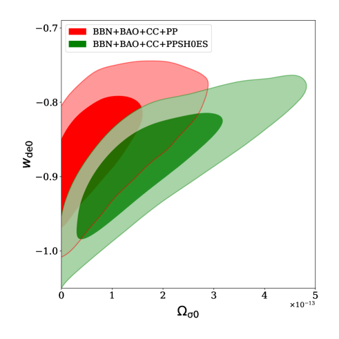
In Table 3, we summarize the observational constraints on free parameters and some derived parameters of the CDM and CDM+ models at CL from two data combinations: BAO+CC+BBN+PP and BAO+CC+BBN+PPSH0ES. The second row over each parameter (mentioned in blue color) represents the constraints at CL on CDM and CDM+ models from same set of data combinations. The upper bounds on anisoptropic expansion parameter, , at CL are of order for CDM+ model with both the data combinations. The upper bounds of for this model read as: and from BAO+CC+BBN+PP and BAO+CC+BBN+PPSH0ES, respectively. On other hand, the upper bounds on anisoptropic expansion parameter for CDM+ model are: and from BAO+CC+BBN+PP and BAO+CC+BBN+PPSH0ES combinations, respectively. Thus, we see that the CDM+ model provides weaker upper bounds on anisotropy parameter by one order of magnitude as compared to CDM+ model with both the data combinations. We observe that anisotropic parameter has a strong positive correlation with DE EoS parameter from both the data combinations. This means that larger amount of anisotropy in the Universe results larger value of DE EoS, see Figure 1.
| Data set | BAO+CC+BBN+PP | BAO+CC+BBN+PP+SH0ES | ||
|---|---|---|---|---|
| Model | CDM | CDM+ | CDM | CDM+ |
| CDM | CDM+ | CDM | CDM+ | |
| 0 | 0 | |||
| 0 | 0 | |||
For the CDM+ model, it can be observed from Table 3 that the DE EoS parameter does not prefer the cosmological constant form of DE (having ) with both data combinations. Also, at CL, the DE EoS parameter ( for BAO+CC+BBN+PP data combination and for BAO+CC+BBN+PPSH0ES data combination) does not prefer the cosmological constant form of DE with both data combinations. For this model, the mean values of DE EoS parameter (at CL as well as CL range), , lie in quintessence region , pointing towards quintessence behaviour of DE with both data combinations. Also, for the CDM model, the mean value of at CL, as shown in Table 3, lies in quintessence region with BAO+CC+BBN+PP data combination whereas, it touches the phantom barrier at CL with the same data combination ( for BAO+CC+BBN+PP data combination). Again, for the same model with BAO+CC+BBN+PPSH0ES data combination, the mean value of lies in phantom region at CL as well as CL. At CL, for BAO+CC+BBN+PPSH0ES data combination. Also, we observe from Figure 2 that finds a strong negative correlation with in case of CDM model whereas slight negative correlation in case of CDM+ model from both the data combinations.
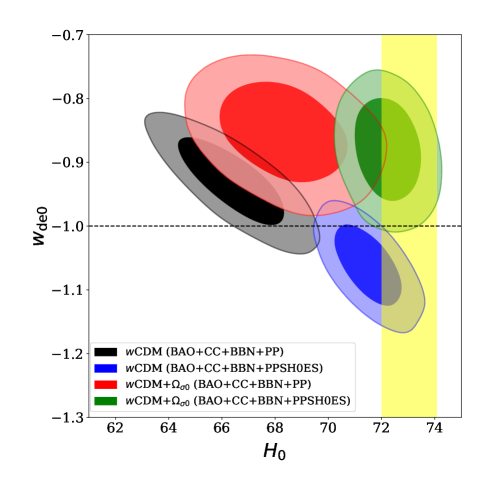
One of the most well known and intriguing puzzle nowadays in cosmology is discrepancy between Planck CMB data within the baseline CDM model and direct local measurements of the current rate of expansion of the Universe (that is, the value of Hubble constant, ), as discussed in Section I. Now, we discuss the constraints on Hubble constant for the considered models and compare the results with the previous work [60]. For BAO+CC+BBN+PP data combination, the constraint on for CDM (CDM) model reads: , and for CDM+ (CDM+) model, it reads: at 68% CL. For BAO+CC+BBN+PP data combination, we have obtained lower mean values of for CDM and CDM+ models as compared to CDM and CDM+ models, respectively. For BAO+CC+BBN+PPSH0ES data combination, the constraint on for CDM (CDM) model reads: , and for CDM+ (CDM+) model, it reads: at 68% CL. Thus, from BAO+CC+BBN+PPSH0ES data CDM model provides higher mean value of as compared to CDM model, whereas CDM+ and CDM+ models provide more or less the same mean values of . The highest value of Hubble constant obtained in the present analysis is from BAO+CC+BBN+PPSH0ES data combinations which is consistent with from SH0ES measurement. Quantifying the tension with SH0ES measurement for BAO+CC+BBN+PP data combination, we found that there is tension on in the CDM model and there is tension on in CDM+ model. Also, for BAO+CC+BBN+PPSH0ES data combination, tension on is observed in CDM model and tension is observed on in CDM+ model. So, for BAO+CC+BBN+PP data combination tension is relieved by in presence of anisotropy of the order with constant EoS parameter of DE. Also, for BAO+CC+BBN+PPSH0ES data combination tension is relieved by in presence of anisotropy of the order with constant EoS parameter of DE. See the Figure 2 where vertical yellow band represents from SH0ES measurement and constraints on in Table 3. Also, from Figure 4, we observe a positive correlation of with with both the data combinations. So, in order to get a larger value of , a larger amount of anisotropy is required.
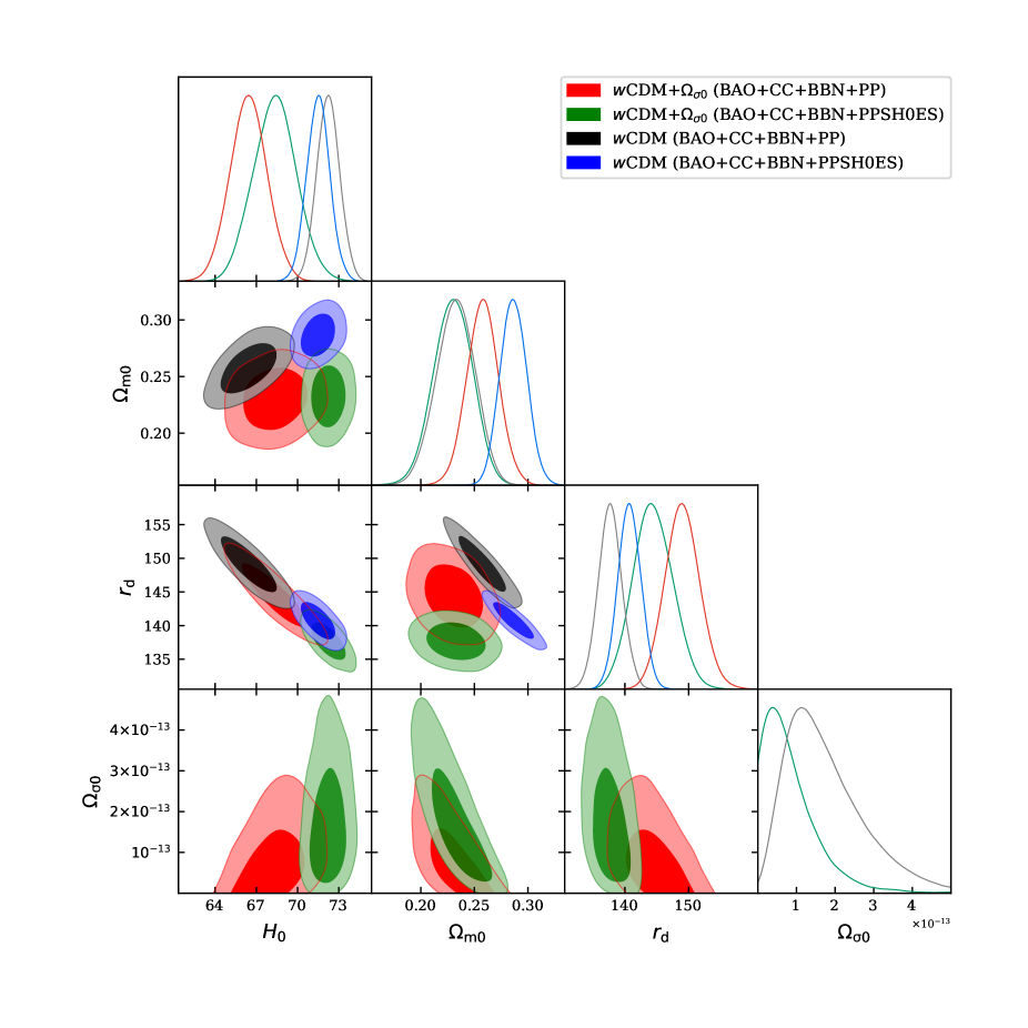
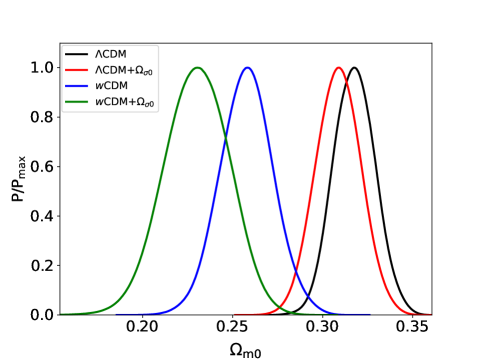
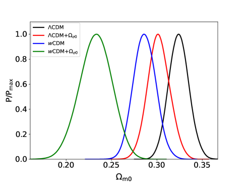
Now, we discuss how and affect the present day matter density parameter, . Firstly, we observe that the CDM model provides significantly lower mean values of as compared to CDM model for both data combinations. Second, adding anisotropy to CDM model slightly reduces the mean value of for both the data combinations.Also, inclusion of anisotropy into the CDM model significantly reduces the mean values of for both the data combinations. The constraints on for CDM model are: and from the data combinations BAO+CC+BBN+PP and BAO+CC+BBN+PPSH0ES, respectively. The constraints on for CDM+ model are: for the data combination BAO+CC+BBN+PP and for the data combination BAO+CC+BBN+PPSH0ES. We can observe the deviations in the distribution of for considered models in one dimensional marginalized probability distribution as shown in Figure 3 (also, see table 3) for both the data combinations. We also observe that parameters, and finds a negative correlation with both data combinations, see parametric space in the Figure 4.
The considered CDM and CDM+ models provides higher values of as compared to CDM and CDM+ models with BAO+CC+BBN+PP data combination. Also, from BAO+CC+BBN+PPSH0ES data combination, we obtain the result that the CDM model prefers a lower value of than CDM model, but CDM+ and CDM+ provide equivalent mean values on with similar error bars. Further, we notice that the addition of anisotropy reduces the value of in both the cases. We can observe from Figure 4, that the parameters and are negatively correlated with both the data combinations, which means that for a small increment in values, there would be corresponding decrement in values.
We have observed that different model parameters are influenced due to anisotropy. For instance, we observe a negative correlation between and which can be seen in Figure 2. Note that parameters influence each other while fitting the multi-parameter space simultaneously [81, 82]. Also, the other parameters of the models under consideration (with constant EoS of DE) are affected by anisotropy in such a way that results into the relieving of the tension up to . It is important to emphasize that in equation (19), the scaling has relevance for the early Universe while it becomes negligible in the late Universe. Thus, the anisotropic model under consideration behaves like the Early DE model. For more about Early DE models, we refer the readers to see the recent and interesting review [33] and references therein.
V Concluding Remarks
In the present work, we have derived CMB independent observational constraints on two simplest extensions of CDM model, namely CDM and CDM+ models from recent data sets including BAO, CC, BBN, PP and PPSH0ES in two combinations: BAO+CC+BBN+PP and BAO+CC+BBN+PPSH0ES. We have obtained that DE EoS parameter favours quintessence form of DE for CDM+ model from both the data combinations at CL as well as CL. For the CDM model, the mean value of at CL lies in quintessence region with BAO+CC+BBN+PP data combination whereas, it touches the phantom barrier at CL with the same data combination. Again, for the same model with BAO+CC+BBN+PPSH0ES data combination, the mean value of lies in phantom region at CL. Also, we notice a strong positive correlation between and anisotropy parameter () with both data combinations, see Figure 1. The upper bounds on are of the order from both the data combinations. The constant EoS of DE significantly affects present day matter density parameter and provides lower values for both the models (as compared to models investigated in [60] with cosmological constant DE) from both the data combinations.
We have obtained higher values of Hubble constant with and at 68% CL for CDM and CDM+ models, respectively with BAO+CC+BBN+PPSH0ES data. The obtained value of in both the considered models from BAO+CC+BBN+PPSH0ES are consistent with SH0ES measurements (), and thus tension is relieved. Further, we notice that inclusion of anisotropy parameter in the CDM model reduces the tension by and with BAO+CC+BBN+PP and BAO+CC+BBN+PPSH0ES data combinations, respectively.
Overall, we have shown that how the anisotropic extensions of standard cosmological model can influence the estimation of , and contribute significantly to the resolution of the tension.
References
- Riess et al. [1998] A. G. Riess et al. (Supernova Search Team), Astron. J. 116, 1009 (1998), arXiv:astro-ph/9805201 .
- Perlmutter et al. [1999] S. Perlmutter et al. (Supernova Cosmology Project), Astrophys. J. 517, 565 (1999), arXiv:astro-ph/9812133 .
- Aghanim et al. [2020] N. Aghanim et al. (Planck), Astron. Astrophys. 641, A6 (2020), [Erratum: Astron.Astrophys. 652, C4 (2021)], arXiv:1807.06209 [astro-ph.CO] .
- Abbott et al. [2019] T. M. C. Abbott et al. (DES), Astrophys. J. Lett. 872, L30 (2019), arXiv:1811.02374 [astro-ph.CO] .
- Blomqvist et al. [2019] M. Blomqvist et al., Astron. Astrophys. 629, A86 (2019), arXiv:1904.03430 [astro-ph.CO] .
- Abbott et al. [2022] T. M. C. Abbott et al. (DES), Phys. Rev. D 105, 023520 (2022), arXiv:2105.13549 [astro-ph.CO] .
- Riechers et al. [2022] D. A. Riechers, A. Weiss, F. Walter, C. L. Carilli, P. Cox, R. Decarli, and R. Neri, Nature 602, 58 (2022), arXiv:2202.00693 [astro-ph.GA] .
- Copeland et al. [2006] E. J. Copeland, M. Sami, and S. Tsujikawa, Int. J. Mod. Phys. D 15, 1753 (2006), arXiv:hep-th/0603057 .
- Bamba et al. [2012] K. Bamba, S. Capozziello, S. Nojiri, and S. D. Odintsov, Astrophys. Space Sci. 342, 155 (2012), arXiv:1205.3421 [gr-qc] .
- Verde et al. [2019] L. Verde, T. Treu, and A. G. Riess, Nature Astron. 3, 891 (2019), arXiv:1907.10625 [astro-ph.CO] .
- Clark et al. [2023] S. J. Clark, K. Vattis, J. Fan, and S. M. Koushiappas, Phys. Rev. D 107, 083527 (2023), arXiv:2110.09562 [astro-ph.CO] .
- Riess et al. [2022] A. G. Riess et al., Astrophys. J. Lett. 934, L7 (2022), arXiv:2112.04510 [astro-ph.CO] .
- Freedman [2017] W. L. Freedman, Nature Astron. 1, 0121 (2017), arXiv:1706.02739 [astro-ph.CO] .
- Mörtsell and Dhawan [2018] E. Mörtsell and S. Dhawan, JCAP 09, 025 (2018), arXiv:1801.07260 [astro-ph.CO] .
- Knox and Millea [2020] L. Knox and M. Millea, Phys. Rev. D 101, 043533 (2020), arXiv:1908.03663 [astro-ph.CO] .
- Di Valentino et al. [2021] E. Di Valentino, O. Mena, S. Pan, L. Visinelli, W. Yang, A. Melchiorri, D. F. Mota, A. G. Riess, and J. Silk, Class. Quant. Grav. 38, 153001 (2021), arXiv:2103.01183 [astro-ph.CO] .
- Vagnozzi [2021] S. Vagnozzi, Phys. Rev. D 104, 063524 (2021), arXiv:2105.10425 [astro-ph.CO] .
- Hu and Wang [2023] J.-P. Hu and F.-Y. Wang, Universe 9, 94 (2023), arXiv:2302.05709 [astro-ph.CO] .
- Pan et al. [2019] S. Pan, W. Yang, E. Di Valentino, E. N. Saridakis, and S. Chakraborty, Phys. Rev. D 100, 103520 (2019), arXiv:1907.07540 [astro-ph.CO] .
- Kumar and Nunes [2016] S. Kumar and R. C. Nunes, Phys. Rev. D 94, 123511 (2016), arXiv:1608.02454 [astro-ph.CO] .
- Kumar and Nunes [2017] S. Kumar and R. C. Nunes, Phys. Rev. D 96, 103511 (2017), arXiv:1702.02143 [astro-ph.CO] .
- Yang et al. [2018] W. Yang, A. Mukherjee, E. Di Valentino, and S. Pan, Phys. Rev. D 98, 123527 (2018), arXiv:1809.06883 [astro-ph.CO] .
- Kumar et al. [2019] S. Kumar, R. C. Nunes, and S. K. Yadav, Eur. Phys. J. C 79, 576 (2019), arXiv:1903.04865 [astro-ph.CO] .
- Kumar [2021] S. Kumar, Phys. Dark Univ. 33, 100862 (2021), arXiv:2102.12902 [astro-ph.CO] .
- Kaeonikhom et al. [2023] C. Kaeonikhom, H. Assadullahi, J. Schewtschenko, and D. Wands, JCAP 01, 042 (2023), arXiv:2210.05363 [astro-ph.CO] .
- Bringmann et al. [2018] T. Bringmann, F. Kahlhoefer, K. Schmidt-Hoberg, and P. Walia, Phys. Rev. D 98, 023543 (2018), arXiv:1803.03644 [astro-ph.CO] .
- Kumar et al. [2018] S. Kumar, R. C. Nunes, and S. K. Yadav, Phys. Rev. D 98, 043521 (2018), arXiv:1803.10229 [astro-ph.CO] .
- Yadav [2019] S. K. Yadav, Mod. Phys. Lett. A 35, 1950358 (2019), arXiv:1907.05886 [astro-ph.CO] .
- Yadav et al. [2023] V. Yadav, S. K. Yadav, and A. K. Yadav, Phys. Dark Univ. 42, 101363 (2023), arXiv:2307.05155 [astro-ph.CO] .
- Poulin et al. [2019] V. Poulin, T. L. Smith, T. Karwal, and M. Kamionkowski, Phys. Rev. Lett. 122, 221301 (2019), arXiv:1811.04083 [astro-ph.CO] .
- Niedermann and Sloth [2020] F. Niedermann and M. S. Sloth, Phys. Rev. D 102, 063527 (2020), arXiv:2006.06686 [astro-ph.CO] .
- Hill et al. [2020] J. C. Hill, E. McDonough, M. W. Toomey, and S. Alexander, Phys. Rev. D 102, 043507 (2020), arXiv:2003.07355 [astro-ph.CO] .
- Poulin et al. [2023] V. Poulin, T. L. Smith, and T. Karwal, Phys. Dark Univ. 42, 101348 (2023), arXiv:2302.09032 [astro-ph.CO] .
- Reeves et al. [2023] A. Reeves, L. Herold, S. Vagnozzi, B. D. Sherwin, and E. G. M. Ferreira, Mon. Not. Roy. Astron. Soc. 520, 3688 (2023), arXiv:2207.01501 [astro-ph.CO] .
- Akarsu et al. [2020] O. Akarsu, J. D. Barrow, L. A. Escamilla, and J. A. Vazquez, Phys. Rev. D 101, 063528 (2020), arXiv:1912.08751 [astro-ph.CO] .
- Akarsu et al. [2021] O. Akarsu, S. Kumar, E. Özülker, and J. A. Vazquez, Phys. Rev. D 104, 123512 (2021), arXiv:2108.09239 [astro-ph.CO] .
- Akarsu et al. [2023a] O. Akarsu, S. Kumar, E. Özülker, J. A. Vazquez, and A. Yadav, Phys. Rev. D 108, 023513 (2023a), arXiv:2211.05742 [astro-ph.CO] .
- Akarsu et al. [2023b] O. Akarsu, E. Di Valentino, S. Kumar, R. C. Nunes, J. A. Vazquez, and A. Yadav, (2023b), arXiv:2307.10899 [astro-ph.CO] .
- Akarsu et al. [2024] O. Akarsu, A. D. Felice, E. D. Valentino, S. Kumar, R. C. Nunes, E. Ozulker, J. A. Vazquez, and A. Yadav, “CDM cosmology from a type-II minimally modified gravity,” (2024), arXiv:2402.07716 [astro-ph.CO] .
- Perivolaropoulos and Skara [2022] L. Perivolaropoulos and F. Skara, New Astron. Rev. 95, 101659 (2022), arXiv:2105.05208 [astro-ph.CO] .
- Abdalla et al. [2022] E. Abdalla et al., JHEAp 34, 49 (2022), arXiv:2203.06142 [astro-ph.CO] .
- Vagnozzi [2023] S. Vagnozzi, Universe 9, 393 (2023), arXiv:2308.16628 [astro-ph.CO] .
- Freedman and Madore [2023] W. L. Freedman and B. F. Madore, JCAP 11, 050 (2023), arXiv:2309.05618 [astro-ph.CO] .
- Yeung and Chu [2022] S. Yeung and M.-C. Chu, Phys. Rev. D 105, 083508 (2022), arXiv:2201.03799 [astro-ph.CO] .
- Hu et al. [2020] J. P. Hu, Y. Y. Wang, and F. Y. Wang, Astron. Astrophys. 643, A93 (2020), arXiv:2008.12439 [astro-ph.CO] .
- Fosalba and Gaztanaga [2020] P. Fosalba and E. Gaztanaga, (2020), 10.1093/mnras/stab1193, arXiv:2011.00910 [astro-ph.CO] .
- Aluri et al. [2023] P. K. Aluri et al., Class. Quant. Grav. 40, 094001 (2023), arXiv:2207.05765 [astro-ph.CO] .
- Watanabe et al. [2009] M.-a. Watanabe, S. Kanno, and J. Soda, Phys. Rev. Lett. 102, 191302 (2009), arXiv:0902.2833 [hep-th] .
- Kanno et al. [2010] S. Kanno, J. Soda, and M.-a. Watanabe, JCAP 12, 024 (2010), arXiv:1010.5307 [hep-th] .
- Akarsu et al. [2019] O. Akarsu, S. Kumar, S. Sharma, and L. Tedesco, Phys. Rev. D 100, 023532 (2019), arXiv:1905.06949 [astro-ph.CO] .
- Akarsu et al. [2023c] O. Akarsu, E. Di Valentino, S. Kumar, M. Ozyigit, and S. Sharma, Phys. Dark Univ. 39, 101162 (2023c), arXiv:2112.07807 [astro-ph.CO] .
- Amirhashchi and Amirhashchi [2019] H. Amirhashchi and S. Amirhashchi, Phys. Rev. D 99, 023516 (2019), arXiv:1803.08447 [astro-ph.CO] .
- Amirhashchi and Amirhashchi [2020] H. Amirhashchi and S. Amirhashchi, Phys. Dark Univ. 29, 100557 (2020), arXiv:1802.04251 [astro-ph.CO] .
- Amirhashchi et al. [2022] H. Amirhashchi, A. K. Yadav, N. Ahmad, and V. Yadav, Phys. Dark Univ. 36, 101043 (2022), arXiv:2001.03775 [astro-ph.CO] .
- Yadav et al. [2021a] A. K. Yadav, A. Alshehri, N. Ahmad, G. Goswami, and M. Kumar, Physics of the Dark Universe 31, 100738 (2021a).
- Yadav et al. [2021b] A. K. Yadav, A. K. Yadav, M. Singh, R. Prasad, N. Ahmad, and K. P. Singh, Physical Review D 104, 064044 (2021b).
- Rahman et al. [2022] W. Rahman, R. Trotta, S. S. Boruah, M. J. Hudson, and D. A. van Dyk, Mon. Not. Roy. Astron. Soc. 514, 139 (2022), arXiv:2108.12497 [astro-ph.CO] .
- Bhardwaj [2023] V. K. Bhardwaj, (2023), arXiv:2308.02864 [gr-qc] .
- Constantin et al. [2023] A. Constantin, T. R. Harvey, S. von Hausegger, and A. Lukas, Class. Quant. Grav. 40, 245015 (2023), arXiv:2212.03234 [astro-ph.CO] .
- Yadav [2023] V. Yadav, Phys. Dark Univ. 42, 101365 (2023), arXiv:2306.16135 [astro-ph.CO] .
- Alam et al. [2021] S. Alam et al. (eBOSS), Phys. Rev. D 103, 083533 (2021), arXiv:2007.08991 [astro-ph.CO] .
- Cooke et al. [2016] R. J. Cooke, M. Pettini, K. M. Nollett, and R. Jorgenson, Astrophys. J. 830, 148 (2016), arXiv:1607.03900 [astro-ph.CO] .
- Bennett et al. [2021] J. J. Bennett, G. Buldgen, P. F. De Salas, M. Drewes, S. Gariazzo, S. Pastor, and Y. Y. Y. Wong, JCAP 04, 073 (2021), arXiv:2012.02726 [hep-ph] .
- Jimenez and Loeb [2002] R. Jimenez and A. Loeb, Astrophys. J. 573, 37 (2002), arXiv:astro-ph/0106145 .
- Zhang et al. [2014] C. Zhang, H. Zhang, S. Yuan, T.-J. Zhang, and Y.-C. Sun, Res. Astron. Astrophys. 14, 1221 (2014), arXiv:1207.4541 [astro-ph.CO] .
- Simon et al. [2005] J. Simon, L. Verde, and R. Jimenez, Phys. Rev. D 71, 123001 (2005), arXiv:astro-ph/0412269 .
- Moresco et al. [2012] M. Moresco et al., JCAP 08, 006 (2012), arXiv:1201.3609 [astro-ph.CO] .
- Moresco et al. [2016] M. Moresco, L. Pozzetti, A. Cimatti, R. Jimenez, C. Maraston, L. Verde, D. Thomas, A. Citro, R. Tojeiro, and D. Wilkinson, JCAP 05, 014 (2016), arXiv:1601.01701 [astro-ph.CO] .
- Ratsimbazafy et al. [2017] A. L. Ratsimbazafy, S. I. Loubser, S. M. Crawford, C. M. Cress, B. A. Bassett, R. C. Nichol, and P. Väisänen, Mon. Not. Roy. Astron. Soc. 467, 3239 (2017), arXiv:1702.00418 [astro-ph.CO] .
- Stern et al. [2010] D. Stern, R. Jimenez, L. Verde, M. Kamionkowski, and S. A. Stanford, JCAP 02, 008 (2010), arXiv:0907.3149 [astro-ph.CO] .
- Borghi et al. [2022] N. Borghi, M. Moresco, and A. Cimatti, Astrophys. J. Lett. 928, L4 (2022), arXiv:2110.04304 [astro-ph.CO] .
- Jiao et al. [2023] K. Jiao, N. Borghi, M. Moresco, and T.-J. Zhang, Astrophys. J. Suppl. 265, 48 (2023), arXiv:2205.05701 [astro-ph.CO] .
- Moresco [2015] M. Moresco, Mon. Not. Roy. Astron. Soc. 450, L16 (2015), arXiv:1503.01116 [astro-ph.CO] .
- Kneller and Steigman [2004] J. P. Kneller and G. Steigman, New J. Phys. 6, 117 (2004), arXiv:astro-ph/0406320 .
- Steigman [2007] G. Steigman, Ann. Rev. Nucl. Part. Sci. 57, 463 (2007), arXiv:0712.1100 [astro-ph] .
- Barrow and Scherrer [2018] J. D. Barrow and R. J. Scherrer, Phys. Rev. D 98, 043534 (2018), arXiv:1803.02383 [astro-ph.CO] .
- Mossa et al. [2020] V. Mossa et al., Nature 587, 210 (2020).
- Brout et al. [2022] D. Brout et al., Astrophys. J. 938, 110 (2022), arXiv:2202.04077 [astro-ph.CO] .
- Blas et al. [2011] D. Blas, J. Lesgourgues, and T. Tram, JCAP 07, 034 (2011), arXiv:1104.2933 [astro-ph.CO] .
- Audren et al. [2013] B. Audren, J. Lesgourgues, K. Benabed, and S. Prunet, JCAP 02, 001 (2013), arXiv:1210.7183 [astro-ph.CO] .
- Marra and Perivolaropoulos [2021] V. Marra and L. Perivolaropoulos, Phys. Rev. D 104, L021303 (2021), arXiv:2102.06012 [astro-ph.CO] .
- Camarena and Marra [2023] D. Camarena and V. Marra, (2023), arXiv:2307.02434 [astro-ph.CO] .