Unveiling Intrinsic Many-Body Complexity by Compressing Single-Body Triviality

Abstract

The simultaneous treatment of static and dynamical correlations in strongly-correlated electron systems is a critical challenge. In particular, finding a universal scheme for identifying a single-particle orbital basis that minimizes the representational complexity of the many-body wavefunction is a formidable and longstanding problem. As a substantial contribution towards its solution, we show that the total orbital correlation actually reveals and quantifies the intrinsic complexity of the wavefunction, once it is minimized via orbital rotations. To demonstrate the power of this concept in practice, an iterative scheme is proposed to optimize the orbitals by minimizing the total orbital correlation calculated by the tailored coupled cluster singles and doubles (TCCSD) ansatz. The optimized orbitals enable the limited TCCSD ansatz to capture more non-trivial information of the many-body wavefunction, indicated by the improved wavefunction and energy. An initial application of this scheme shows great improvement of TCCSD in predicting the singlet ground state potential energy curves of the strongly correlated C₂ and Cr₂ molecule.

I Introduction

The ab-initio simulation of strongly correlated systems is a critical challenge in quantum chemistry [1, 2] and materials science [3, 4, 5]. More specifically, this problem is complicated by the intricate interplay between the so-called static and dynamical electron-electron correlations. The former exhibits itself in the presence of many significant many-body configurations, or in the case of matrix product state (MPS), the very high bond dimensions, needed to even qualitatively describe the wavefunction. The latter includes the remaining correlation effects, such as those related to the short-range Kato cusp condition [6], long-range electron-electron screening effects [7, 8, 9, 10], van der Waals interactions [11, 12, 13] etc. Towards solving this problem, recent years have witnessed promising developments of a plethora of methods, including tensor network theories [14, 15, 16], quantum Monte Carlo methods [17, 18, 19, 20, 21], quantum chemical theories, such as specific perturbation theories [22, 23, 24, 25], coupled cluster (CC) [26, 27, 28, 29, 30] and functional theories [31, 32, 33, 34]. Each of these methods covers certain pieces of the strong correlation puzzle. Ongoing efforts are focussed on utilizing combinations of them to reach larger areas of the correlation landscape [35, 36, 37, 38, 39, 40, 41], while maintaining a delicate balance between accuracy and efficiency. In face of the complexity of the total electron correlation problem, it is surprising that the pivotal role of the underlying single-particle orbital basis is neither fully appreciated nor conclusively understood yet.

For systems dominated by dynamical correlations, the choice of the orbitals influences more the efficiency than the accuracy: Typically, orbitals from cost-effective mean-field theories like Hartree-Fock (HF) and density functional theory (DFT) are used to construct correlated many-body wavefunction ansätze; Natural orbitals, introduced by Löwdin [42], are also commonly used for a more compact Slater determinant expansion in configuration interaction (CI), CC [43, 44, 45, 46], and explicitly correlated methods [47, 48, 49, 50, 51]; Localized orbitals [52, 53] are often used to achieve linear scaling with system size, exploiting the entanglement area law in gapped systems [54, 55, 56].

In systems with strong static correlations, such as systems containing transition metal elements with partially filled $d$-shells, the choice of orbitals can significantly impact not only the efficiency, but, more importantly, the accuracy. It is well recognized that the choice of the single-particle orbitals affects the representational complexity of the many-body wavefunction, e.g. in the context of density matrix renormalization group (DMRG) [57] and full configuration interaction quantum Monte Carlo (FCIQMC) [58]. A badly chosen orbital basis can lead to an artificially difficult computational problem. For example, HF orbitals are normally too delocalized to capture strongly correlated physics, such as strong on-site Coulomb interactions and spin fluctuations. An important advancement was the introduction of the complete active space (CAS) self-consistent field (CASSCF) method [59, 60], where both the orbitals and the CI coefficients in the active space are optimized simultaneously. Another popular choice are the natural orbitals (NO) from computationally efficient methods [51, 61, 37]. For a comprehensive review of the active space orbital construction and selection methods, we refer to Ref. [62] and the references therein .

As a key motivation for our work, we recall that none of the aforementioned orbitals are optimal for the total correlation problem as they are optimized for either static or dynamical correlations, but not for both. Some recognition of the importance of optimizing orbitals by taking into account both types of correlations exists at the single reference methods level [64, 28]. Yet, a general scheme that can be easily extended to other higher-level theories is still missing. The main reason for this is the lack of a concise tool that allows one to quantify the intrinsic complexity of the many-body wavefunction universally, i.e., independently of the underlying ansätze. Inspired by previous work using effective quantum information concepts in quantum chemistry [65, 66, 67, 68, 69, 70], it will be the accomplishment of our work to provide exactly this missing tool. To be more specific, we will establish the total orbital correlation as a quantitative means to link the single-particle basis and the many-body wavefunction’s representational complexity. In particular, we will demonstrate for the first time that through minimizing the total orbital correlation one can systematically reduce the representational complexity, and hence reveal the intrinsic complexity of the many-body wavefunction. In practice, this leads to an improved accuracy of approximate ansätze like TCCSD for strongly correlated systems, as we will show in the exemplary study of the C₂ and Cr₂ molecule.

II Theory

To establish the total orbital correlation as a quantitative means for describing the representational complexity of the many-body wavefunction, we first introduce some basic quantum information concepts, along with an illustrative example. Given an orbital basis $\mathcal{B}$, and a particle number and spin conserving ground state wavefunction $\ket{\Psi}$, we can always perform the following Schmidt decomposition with respect to the bipartition between an orbital $i$ and the rest of the orbitals, $\ket{\Psi}=\sum_{k={0,\uparrow,\downarrow,\uparrow\downarrow}}\sqrt{\lambda^{(i)}_{k}}\ket{k}_{i}\otimes\ket{\psi_{k}}_{\backslash\{i\}}$, where $\lambda^{(i)}_{k}$ are the eigenvalues of the reduced density matrix $\rho_{i}$ of orbital $i$ defined as $\rho_{i}=\mathrm{Tr}_{\backslash\{i\}}[\ket{\Psi}\bra{\Psi}]$. Accordingly, the entropy of orbital $i$ follows as

$$S(\rho_{i})\equiv-\mathrm{Tr}[\rho_{i}\log\rho_{i}]=-\sum_{k={0,\uparrow,\downarrow,\uparrow\downarrow}}\lambda^{(i)}_{k}\log\lambda^{(i)}_{k},$$ (1)

which quantifies for pure states precisely the entanglement between orbital $i$ and the rest of the orbitals, or equivalently (up to a factor $1/2$) the entire correlation including both quantum and classical contributions[71, 72]. It is worth noticing here that the eigenvalues $\lambda_{k}^{(i)}$ change as $\mathcal{B}$ is varied. This can easily be seen when they are expressed as functions of the one- and two-particle reduced density matrix (1-RDM and 2-RDM) [66, 70, 73]. Moreover, the total orbital correlation describes the correlation of various $M$ orbitals in $\mathcal{B}$ collectively. To be more specific, it quantifies through the quantum relative entropy $S(\rho||\sigma)\equiv\mathrm{Tr}[\rho(\log(\rho)-\log(\sigma))]$ the deviation of the quantum state $\rho=|\Psi\rangle\langle\Psi|$ to the manifold of states with zero correlation between various orbitals in $\mathcal{B}$, i.e.,

$$I_{\mathrm{tot}}^{(\mathcal{B})}(\rho) = \min_{\sigma\equiv\sigma_{1}\otimes\ldots\otimes\sigma_{d}}S\big{(}|\Psi\rangle\langle\Psi|\big{|}\big{|}\sigma\big{)}$$ (2)

$$= \sum_{i=1}^{M}S(\rho_{i})$$

In the last line, we used the well-know fact [74] that the minimum in the first line is attained for the uncorrelated state given by the product of the single orbital reduced density matrices $\rho_{i}$ of $|\Psi\rangle$.

In order to illustrate how total orbital correlation directly reflects the multiconfigurational character of a wavefunction $\ket{\Psi}$, we first consider a two-electron singlet state in two orbitals. In this case, the Shannon entropy of the CI coefficients of the many-body wavefunction expanded in the four configurations $\{\ket{0,\uparrow\downarrow},\ket{\uparrow,\downarrow},\ket{\downarrow,\uparrow},\ket{\uparrow\downarrow,0}\}$ is defined as $H(\{|c_{i}|^{2}\})=-\sum_{i=1}^{4}|c_{i}|^{2}\log(|c_{i}|^{2})$ which actually equals (up to a prefactor) the total orbital correlation (2). In particular, when the total orbital correlation is 0, the state $\ket{\Psi}$ is a single Slater determinant, whereas when it is maximal, $\ket{\Psi}$ is also maximally multiconfigurational. Remarkably, the total orbital correlation of $\ket{\Psi}$ can vary drastically when the orbital basis changes.

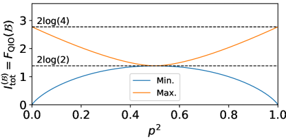
Figure 1: Minimal and maximal total orbital correlation, Eq. (2), over all real orbital bases $\mathcal{B}$ for a two electron singlet state $\ket{\Psi}=p\ket{\uparrow\downarrow,0}+\sqrt{1-p^{2}}\ket{0,\uparrow\downarrow}$ against $p^{2}$.

One can verify that it attains its minimal value for the natural orbitals of $\ket{\Psi}$ (which are in general not the minimizer), where $\ket{\Psi}$ can be expressed as a zero-senority state $\ket{\Psi}=p\ket{\uparrow\downarrow,0}+\sqrt{1-p^{2}}\ket{0,\uparrow\downarrow}$, where we use $p$ to denote the CI coefficient of the first configuration in the natural orbital basis. We therefore define the single-body triviality as any redundant orbital correlation beyond the minimal total orbital correlation, as shown as the blue curve in Fig. 6. When $p^{2}$ is closed to 0 or 1, $\ket{\Psi}$ is of single reference character, and correspondingly the difference of the total orbital correlation between the “best” and “worst” choice of orbital basis is radical. When $p^{2}=1/2$, the state is equally and maximally multiconfigurational in every orbital basis, which means there is no single-body triviality in the state. For more details on this example, we refer to the Appendix B.

Based on the analytic insights above, and the precise meaning of the total orbital correlation, we propose the following cost function for orbital optimization

$$F_{\mathrm{QIO}}(\mathcal{B})\equiv I_{\mathrm{tot}}^{(\mathcal{B})}(\rho)=\sum_{i=1}^{M}S(\rho_{i}),$$ (3)

where $M$ is the total number of spatial orbitals. The cost function is 0 when the wavefunction is a single Slater determinant, and achieves the maximal value of $M\log 4$ when the wavefunction is maximally multiconfigurational.

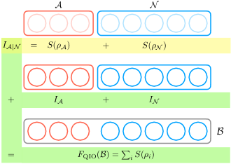
Figure 2: Illustration of coarse-grained and finest-grained orbital correlation, and the associating sum rules.

To provide more evidence for the distinct suitability of our cost function (3), let us first consider instead of the finest split a coarser partitioning $\Pi\equiv\mathcal{S}_{1}|\ldots|\mathcal{S}_{R}$ of the orbital basis $\mathcal{B}$. As an extension of Eq. (2), for any quantum state $\rho$ the correlation between various subsystems $\mathcal{S}_{J}$ is quantified by $I_{\Pi}(\rho)=\sum_{J=1}^{R}S(\rho_{J})-S(\rho).$ Here $\rho_{J}$ is the orbital reduced state of subsystem $\mathcal{S}_{J}$ including all orbitals $i\in\mathcal{S}_{J}$. This coarse-grained correlation vanishes indeed if and only if the total state $\rho$ takes the form of a product of reduced states $\rho_{J}$ of various subsystems $\mathcal{S}_{J}$. Yet, $I_{\Pi}(\rho)$ is therefore not capable of detecting any correlation within any of the subsystems $\mathcal{S}_{J}$, in striking contrast to our cost function (3) which refers to the finest partitioning of $\mathcal{B}$. To put this into context, we consider the partitioning of the orbitals into active and non-active spaces. We denote the subset of active orbitals as $\mathcal{A}$, and its complement, i.e. the subset of non-active orbitals as $\mathcal{N}$. Then $I_{\mathcal{A}}$ and $I_{\mathcal{N}}$ quantify the internal total correlation within the active and non-active subspaces, respectively. At the same time, the correlation between the two subspaces is quantified as $I_{\mathcal{A}|\mathcal{N}}=S(\rho_{\mathcal{A}})+S(\rho_{\mathcal{N}}).$ Therefore, $F_{\mathrm{QIO}}$ can be decomposed as

$$F_{\mathrm{QIO}}(\mathcal{B})=I_{\mathcal{A}|\mathcal{N}}+I_{\mathcal{A}}+I_{\mathcal{N}}.$$ (4)

Accordingly, as a key insight of our work, minimizing $F_{\mathrm{QIO}}(\mathcal{B})$ means nothing else than reducing simultaneously the correlation between the active space and the non-active space, as well as within these two subspaces.

Also from a practical point of view, our cost function is particulary suitable. To explain this, we first recall that in certain scenarios, for instance DMRG, the entropy of blocks containing more than one orbital can be efficiently exploited for orbital optimization due to the unique structure of the ansatz [57]. But, in general, going beyond the current partition will require higher order RDMs, which is computationally expensive for ansätze that do not possess the special structure of an MPS.

After having presented all these appealing features of our proposed cost function (3), one may wonder which orbitals its minimization will actually yield. Providing a comprehensive analytical answer is out of reach due to the huge complexity of the electron correlation problem and the form of (3). Yet, we recall a remarkable observation made in Ref. [75]. There, they considered our cost function (3) for spinless fermions, or equivalently for spinful fermions the finest splitting of the entire one-particle Hilbert space rather than the orbital one-particle Hilbert space. In that case, the minimization leads to the natural spin-orbitals, i.e., the eigenstates of the full 1-RDM still including spin-information. In our case, however, the ideas of the derivation in [75] do not apply anymore. Hence, the spatial orbitals minimizing our cost function (3), termed QIOs, will not coincide with the natural orbitals but they could be quite similar, at least for some systems. In that sense, our work may provides a quite surprising alternative characterization of the natural orbitals: They approximately but not exactly minimize the total orbital correlation in a $N$-electron wavefunction. Because of this, we will also consider the spatial natural orbitals in this work together with the orbitals obtained by minimizing (3).

Based on the above considerations, we conclude that Eq (3) is ideal for minimizing the representational complexity of the many-body wavefunction from both a theoretical and practical point of view. In the remainder of the Letter, we will use the term orbital to refer to spatial orbital only.

To turn the above theoretical insights into practical use, it is critical to calculate the 1- and 2-RDM in a both efficient and accurate way in the whole orbital space. Low-bond DMRG was used in previous studies [67, 73] for this purpose. However, in practice this approach becomes computationally expensive when the system size increases. In this Letter, we propose to use the tailored CCSD ansatz (TCCSD) [76]. This enables us to obtain the 1- and 2-RDM efficiently in the whole orbital space, as well as incorporate static and dynamical correlations simultaneously. We stress that TCCSD is used as an example and the theoretical framework in this work can be generalized easily to other ansätze.

II.1 TCCSD

TCCSD [76] was introduced to overcome the shortcomings of CCSD, namely its inadequacy at treating multireference systems, while retaining its merits at capturing dynamical correlations. Here, we focus on TCCSD paired with the complete active space CI (CASCI) solver and on the singlet ground state. First, a FCI calculation in a predefined CAS space size of ($n^{\rm CAS}_{e},n^{\rm CAS}_{o}$) is performed, where $n^{\rm CAS}_{e}$ and $n^{\rm CAS}_{o}$ are the number of electrons and spatial orbitals in the CAS space, respectively. This provides the $T_{1}^{\rm CAS}$ and $T_{2}^{\rm CAS}$ amplitudes in the CAS space. Then the TCCSD ansatz reads $\ket{\Psi_{\rm TCCSD}}=\exp(\hat{T}_{1}^{\rm CAS}+\hat{T}_{2}^{\rm CAS}+\hat{T}_{1}^{\rm ext}+\hat{T}_{2}^{\rm ext})\ket{D_{0}},$ where $\hat{T}_{1}^{\rm CAS}$ and $\hat{T}_{2}^{\rm CAS}$ are the excitation operators in the CAS space, and $\hat{T}_{1}^{\rm ext}$ and $\hat{T}_{2}^{\rm ext}$ contain the rest of the excitations. While solving the CCSD amplitudes equations, we keep the $T_{1}^{\rm CAS}$ and $T_{2}^{\rm CAS}$ amplitudes fixed and allow the $T_{1}^{\rm ext}$ and $T_{2}^{\rm ext}$ amplitudes to be optimized. We refer to Ref. [76] for more details. Here, we resort to the following efficient scheme to calculate the 1- and 2-RDM, without solving for the left eigenstate:

$$\gamma^{p}_{q} =\braket{\Psi_{\rm CISD}}{\hat{a}^{\dagger}_{p}\hat{a}_{q}}{\Psi_{\rm CISD}},$$ (5)

$$\Gamma^{pq}_{rs} =\braket{\Psi_{\rm CISD}}{\hat{a}^{\dagger}_{p}\hat{a}^{\dagger}_{q}\hat{a}_{r}\hat{a}_{s}}{\Psi_{\rm CISD}},$$

where we define $\Psi_{\rm CISD}=\frac{1}{C}(\ket{D_{0}}+\sum_{i,a}T_{i}^{a}\ket{D_{i}^{a}}+\sum_{i,j,a,b}(T_{ij}^{ab}+\frac{1}{2}T^{a}_{i}T^{b}_{j})\ket{D_{ij}^{ab}})$, which is normalized to 1 by $C$. The amplitudes are taken directly from the TCCSD ansatz, including the active and external parts. We stress that this symmetric expression is crucial for maintaining the positive semi-definiteness of the 1-RDM during orbital rotations.

Figure 3: Flowchart of the QIO optimization algorithm. See the main text and the Supplemental Material for more details.

Figure 4: TCCSD-QIO optimization of C₂ at the bond length of 6.0 Bohr (3.175 ${\rm\AA}$) in the cc-pVDZ basis set. An active space size of (8,8) is used. The inset shows the distance between the TCCSD 2-RDM and that of a nearly exact DMRG calculation, defined as $\Delta D=\sqrt{\sum_{pqrs}|\Delta\Gamma^{pq}_{rs}|^{2}}$. The DMRG calculation is performed using the Block2 code [77].

II.2 QIO Optimization Algorithm

An iterative algorithm, consisting of macro and micro cycles as shown in Fig. 3, is employed to find the optimal orbitals by minimizing the cost function in Eq. (3). The algorithm is initialized normally with the HF orbitals at the beginning. The minimization of the cost function is achieved by a quasi-Newton method, of which the details are presented in Appendix 22. The convergence of the macro cycle is reached when the change in the total energy is smaller than a threshold. For comparison, we also carry out an iterative construction of the natural orbitals, substituting the step where we minimize the cost function with the step where we diagonalize the 1-RDM to obtain NOs.

III Results

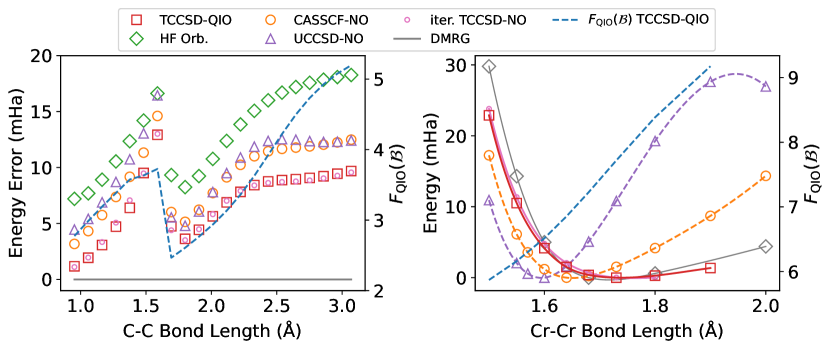
Figure 5: (Left) TCCSD energy errors relative to nearly exact DMRG results [78] along the C₂ dissociation curve using various orbitals in the cc-pVDZ basis set. An active space size of (8,8) is used. (Right) Cr₂ potential energy curves, calculated by TCCSD and DMRG [61] in the cc-pVDZ-DK basis set. All energy curves are shifted by their respective lowest data points and are fitted using the cubic spline method. Entropies in the QIOs are shown in a blue dashed line.

An example of the QIO algorithm in action is shown in Fig. 4 for the orbital optimization of the C₂ at the bond length of 6.0 Bohr (3.175 ${\rm\AA}$) in the cc-pVDZ basis set. See C for the example on the Cr₂ molecule. Only macro iterations are shown, the micro iterations which minimize the cost function $F_{\rm QIO}$ are not presented. An active space size of (8,8) is used. Starting from the HF orbitals, the total total orbital correlation $F_{\rm QIO}$ initially drops at the first macro iteration, then increases as the macro iterations proceed. Correspondingly, the total TCCSD energy first increases and then decreases. At first sight, it is counterintuitive that the total entropy increases as the macro iterations proceed, since the algorithm is designed to minimize the entropy. Indeed, inside each macro iteration, when the orbitals are rotated in several micro iterations, the entropy is minimized. But at the beginning of the next macro iteration, after the correlated ansatz is built anew in the new orbital basis, the value of the entropy increases. We interpret this increase as a gain of non-trivial information on the many-body wavefunction level, after trivial information in the single-particle orbitals is compressed by the minimization. This claim can be supported by the improved wavefunction quality quantified by the distance between the TCCSD 2-RDM and that of a nearly exact DMRG calculation. The distance between the two 2-RDMs is defined as $\Delta D=\sqrt{\sum_{pqrs}|\Delta\Gamma^{pq}_{rs}|^{2}}$ where $\Delta\Gamma=\Gamma^{\rm TCCSD}-\Gamma^{\rm DMRG}$ and $q,p,r,s$ refer to the indices of atomic orbitals. In the inset of Fig. 4, we show that the distance indeed decreases as the macro iterations proceed. Since TCCSD is not variational, a lower energy cannot be taken as better for granted. The reduced error in 2-RDM also justifies that the final decreased TCCSD energy is improved compared to the initial one.

We now turn to the TCCSD energy errors using various orbitals along the dissociation curve in Fig. 5 (Left). The total entanglement entropy is also shown in the optimized orbitals. All calculations are performed in the cc-pVDZ basis set, the same as in the reference DMRG calculations from Ref. [78]. Overall, the errors in the TCCSD energies using QIOs are smaller than those using HF orbitals, CASSCF-NOs and spin-averaged unrestricted CCSD natural orbitals (UCCSD-NOs). As suspected, the CASSCF-NOs, which provide the lowest active space energy, are not the optimal for the total correlation. Remarkably, in a large region along the dissociation curve, the improvement in the total energy from CASSCF-NOs/UCCSD-NOs to QIOs is as substantial as that from HF orbitals to the former. This highlights the importance of the simultaneous consideration of static and dynamical correlations in orbital optimization. As expected, the iterative TCCSD-NO results follow the QIO’s closely, with small deviations around the equilibrium bond length. We observe that the total entropy increases as the bond length increases, until it suddenly drops at the level crossing point, then increases again. We point out that the total entropy is an useful indicator of the complexity of the wavefunction, e.g. it signals the level crossing point, but its value cannot be used to predict the accuracy of the TCCSD energy directly, as shown in Fig. 5 (Left). At very stretched bond lengths, the entanglement entropy is indeed larger than those at shorter bond lengths, in agreement with the intuition that the wavefunction has more multireference character at dissociation.

In Fig. 5 (Right), we show the potential energy curves of Cr₂ around the equilibrium point, calculated by TCCSD using different orbitals along with the exact DMRG results [61] in the cc-pVDZ-DK basis set. The relativistic effects are treated by using the scalar relativistic exact two-component (X2C) Hamiltonian [79, 80] as implemented in PySCF [81]. A minimal active space of (12,12) is used in TCCSD calculations. All curves are shifted by their respective lowest data points. This system has attracted extensive studies over the years [82, 83, 84, 85, 86, 87, 88, 89, 61], and serves as a benchmark for the performance of various methods at handling strong correlations. Even around the equilibrium bond length, the ground state exhibits strong multireference characters, and to capture the shallow potential well requires also the inclusion of dynamical correlations. We note in passing that a previous study employing TCCSD has shown rather unsatisfactory results [89], i.e. a too steep potential energy well, which makes it a perfect test for QIOs.

First, we use UCCSD-NOs as done in DMRG [61]. With these orbitals, TCCSD energies yield a significantly shorter equilibrium bond length of 1.595 ${\rm\AA}$, compared to the exact DMRG result of 1.722 ${\rm\AA}$, with increasingly larger errors as the bond length increases, resulting a very steep potential well. The TCCSD energies using CASSCF-NOs are better than using UCCSD-NOs, with a predicted equilibrium bond length of 1.651 ${\rm\AA}$. However, it yields qualitatively wrong shape of the dissociation curve at shorter and longer bond lengths, resulting still a too steep potential well. TCCSD in the QIOs, on the other hand, captures correctly the shallow potential well around the equilibrium point and in general improves the curve both at shorter and longer bond lengths. Especially, the equilibrium bond length predicted by TCCSD using QIO is 1.737 ${\rm\AA}$, which agrees well with the DMRG result. Most interestingly, we see a difference between the TCCSD-NO and TCCSD-QIO results at slightly stretched bond lengths: the former does not produce a bounded potential energy curve up until 1.8 ${\rm\AA}$, after which the iterative TCCSD-NO algorithm becomes unstable and diverges. The difference in the TCCSD energies between two stretched bond lengths is very small, therefore this unbounded behavior is more evident when we examine the energies values directly, listed in Appendix D.

As noted in Ref. [61], the ground state around 2.25 ${\rm\AA}$ is particularly difficult to capture even with very high bond dimensions in DMRG. We also observe that starting from 2.0 ${\rm\AA}$, the TCCSD iterations in the QIO optimizations do not converge to the threshold of $10^{-6}$ in energy and the TCCSD energies oscillate between macro iterations. Therefore, we do not show the TCCSD-QIO results at bond lengths larger or equal than 2.0 ${\rm\AA}$. This likely underscores the limitations of the TCCSD ansatz with a minimal active space to represent state with very strong multireference character, rather than indicating shortcomings in the QIO algorithm itself. The entropy of the QIOs is shown as a blue dashed line in Fig. 5 (Right). Its smooth increase with the bond length hints at the increasing multireference character of the wavefunction, and serves as an indicator if unphysical results are obtained in the TCCSD calculations when going to larger bond lengths. As pointed out in previous studies on Cr₂ [85, 87, 61], to capture qualitatively correct the whole potential energy curve, a larger active space is needed.

IV Conclusion

We introduced a quantum information-based orbital (QIO) optimization scheme, emerging from a fresh perspective on one of the crucial steps — orbital optimization — in solving the strongly correlated many-body problem. The QIOs are characterized as those orbitals that minimize the total orbital correlation. Accordingly, they reveal the intrinsic complexity of the many-body wavefunction by compressing all trivial information into single-particle orbitals. Due to its distinctive nature, our scheme addresses the challenging task of concurrently treating both static and dynamical correlations in strongly correlated systems by optimizing orbitals considering both types of correlations. By employing our orbital optimization scheme within the TCCSD framework, we obtained superior results compared to other commonly used orbitals. The iterative orbital optimization also provides, to some extent, self-consistent feedback between the active and external space treated separately by CASCI and CCSD, which addresses partially the long-standing issue of the lack of self-consistency in the TCCSD framework. Through the lens of total orbital correlation, we also explained and demonstrated the close relationship between the QIOs and iteratively constructed NOs. The QIOs use information from both the 1- and 2-RDM, so we suspect that in more challenging cases where the two-body cumulant is non-negligible, these two types of orbitals will differ more significantly, hinted by the Cr₂ case. In the future, we hope to extend this algorithm to other systematically improvable methods, such as auxiliary-field quantum Monte Carlo (AFQMC) [87, 21, 20], as well as to spin states beyond singlets. A current bottleneck in TCCSD is the limited active space size that can be treated by CASCI, which can straightforwardly be overcome by using DMRG [90] or FCIQMC [37] as the active space solver. Given the demonstrated advantages of QIOs and the comparable computational cost of QIO to CASSCF, we believe that the QIO algorithm may lead to a change of paradigm in how we approach strongly correlated many-electron systems.

V Acknowledgement

We thank Huanchen Zhai and Seunghoon Lee for useful discussions on DMRG and TCCSD. We are also grateful to Ali Alavi, Daniel Kats, Stefan Knecht and Giovanni Li Manni for comments. We acknowledge financial support from the German Research Foundation (Grant SCHI 1476/1-1), the Munich Center for Quantum Science and Technology, and the Munich Quantum Valley, which is supported by the Bavarian state government with funds from the Hightech Agenda Bayern Plus.

Appendix A Analytic Gradients, Hessians and Quasi-Newton Algorithm

The objective here is to minimize the sum of orbital entropy of all orbitals, amounting to the following cost function

$$F_{\mathrm{QI}}(\mathcal{B})=\sum_{i=1}^{D}S(\rho_{i})$$ (6)

Let $\mathbf{B}$ be the matrix of molecular orbital coefficients where each column corresponds to a molecular orbital. Then the transformation from the initial orbital basis $\mathbf{B}_{0}$ to the minimizing orbital basis $\mathbf{B}_{\mathrm{opt}}$ can be achieved by a unitary transformation $\mathbf{U}_{\mathrm{opt}}=\exp(\mathbf{X}_{\mathrm{opt}})$ as

$$\mathbf{B}_{\mathrm{opt}}=\mathbf{B}_{0}\mathbf{U}^{\dagger}_{\mathrm{opt}}.$$ (7)

With the initial orbital basis fixed, e.g. the HF basis, we can denote all orbital bases by the corresponding real-value unitary $\mathbf{U}$ or its generator, namely a skew-symmetric matrix $\mathbf{X}$. The set of skew-symmetric matrices can be parameterized as

$$\mathbf{X}=\sum_{i<j}x_{ij}\mathbf{A}^{(ij)}$$ (8)

where where $\mathbf{A}^{(ij)}$ is an antisymmetric matrix with elements $A^{(ij)}_{ij}=-A^{(ij)}_{ji}=1$ and otherwise 0. The cost function can be reparameterized as

$$F_{\mathrm{QI}}(\mathcal{B})\equiv F_{\mathrm{QI}}(\mathbf{B})=F_{\mathrm{QI}}(\mathbf{B}_{0}(e^{\mathbf{X}})^{\dagger})\equiv F_{\mathrm{QI}}(\mathbf{X}).$$ (9)

At a local extremum, $F_{\mathrm{QI}}(\mathbf{X}_{\mathrm{opt}})$ satisfies the following extremal conditions

$$\begin{split}&\quad\frac{\partial F_{\mathrm{QI}}}{\partial x_{ij}}(\mathbf{X}_{\mathrm{opt}})\\ &=\lim_{\theta\rightarrow 0}\frac{F_{\mathrm{QI}}(\mathbf{X}_{\mathrm{opt}}\!+\!\theta\mathbf{A}^{(ij)})\!-\!F_{\mathrm{QI}}(\mathbf{X}_{\mathrm{opt}})}{\theta}=0,\end{split}$$ (10)

for all tuples $(i,j)$ such that $i<j$. In practice, the translation invariance of the underlying $D(D-1)/2$ dimensional real space can be exploited to simplify the exponential. To be more specific, one can set the current matrix $\mathbf{X}$ to be the origin at every gradient step, which is the same as constantly updating the reference orbital basis $\mathbf{B}_{0}$. In that case, the derivative of the cost function simplifies to

$$\frac{\partial F_{\mathrm{QI}}}{\partial x_{ij}}(\mathbf{0})=\lim_{\theta\rightarrow 0}\frac{F_{\mathrm{QI}}(\theta\mathbf{A}^{(ij)})\!-\!F_{\mathrm{QI}}(\mathbf{0})}{\theta}.$$ (11)

The infinitesimal unitary transformation $\mathbf{J}^{(ij)}(\theta)=e^{\theta\mathbf{A}^{(ij)}}$ associating to this derivative is simply a Jacobi rotation between orbital $i$ and $j$:

$$\begin{split}(\mathbf{J}^{(ij)}(\theta))_{ii}&=\phantom{-}\cos(\theta),\\ (\mathbf{J}^{(ij)}(\theta))_{ij}&=\phantom{-}\sin(\theta),\\ (\mathbf{J}^{(ij)}(\theta))_{ji}&=-\sin(\theta),\\ (\mathbf{J}^{(ij)}(\theta))_{jj}&=\phantom{-}\cos(\theta),\end{split}$$ (12)

and $(\mathbf{J}^{(ij)}(\theta))_{kl}=\delta_{kl}$ for $k,l\neq i,j$. The derivatives of $F_{\mathrm{QI}}$ can be further broken down using the chain rule

$$\begin{split}\frac{\partial F_{\mathrm{QI}}}{\partial x_{ij}}(\mathbf{0})=-\sum_{i=1}^{D}\sum_{k=0}^{3}\log(\lambda_{k}^{(i)}(\mathbf{0}))\frac{\partial\lambda_{k}^{(i)}}{\partial x_{ij}}(\mathbf{0}),\end{split}$$ (13)

where

$$\begin{split}\lambda_{0}^{(i)}(\mathbf{X})&=1-\gamma(\mathbf{X})^{i}_{i}-\gamma(\mathbf{X})^{\bar{i}}_{\bar{i}}+\Gamma(\mathbf{X})^{i\bar{i}}_{i\bar{i}},\\ \lambda_{1}^{(i)}(\mathbf{X})&=\gamma(\mathbf{X})^{i}_{i}-\Gamma(\mathbf{X})^{i\bar{i}}_{i\bar{i}},\\ \lambda_{2}^{(i)}(\mathbf{X})&=\gamma(\mathbf{X})^{\bar{i}}_{\bar{i}}-\Gamma(\mathbf{X})^{i\bar{i}}_{i\bar{i}},\\ \lambda_{3}^{(i)}(\mathbf{X})&=\Gamma(\mathbf{X})^{i\bar{i}}_{i\bar{i}}.\end{split}$$ (14)

Here, $\gamma(\mathbf{X})$ and $\Gamma(\mathbf{X})$ are the 1- and 2-RDMs in the rotated basis given by

$$\begin{split}\gamma(\mathbf{X})^{i}_{i}&=\sum_{ab}(e^{\mathbf{X}})_{ia}(e^{\mathbf{X}})_{ib}\gamma(\mathbf{0})^{a}_{b},\\ \Gamma(\mathbf{X})^{i\bar{i}}_{i\bar{i}}&=\sum_{abcd}(e^{\mathbf{X}})_{ia}(e^{\mathbf{X}})_{ib}(e^{\mathbf{X}})_{ic}(e^{\mathbf{X}})_{id}\Gamma(\mathbf{0})^{a\bar{b}}_{c\bar{d}},\end{split}$$ (15)

Eventually, their derivatives at $\mathbf{0}$ can be computed from the partial derivatives of the unitary

$$\begin{split}\left.\frac{\partial\exp(\mathbf{X})}{\partial x_{ij}}\right|_{\mathbf{X}=\mathbf{0}}=\lim_{\theta\rightarrow 0}\frac{\mathbf{J}^{(ij)}(\theta)-\openone}{\theta}=(\mathbf{J}^{(ij)})^{\prime}({0})\end{split}$$ (16)

where

$$\begin{split}(\mathbf{J}^{(ij)})^{\prime}({0})_{ii}&=\phantom{-}0,\\ (\mathbf{J}^{(ij)})^{\prime}({0})_{ij}&=\phantom{-}1,\\ (\mathbf{J}^{(ij)})^{\prime}({0})_{ji}&=-1,\\ (\mathbf{J}^{(ij)})^{\prime}({0})_{jj}&=\phantom{-}0,\end{split}$$ (17)

with $(\mathbf{J}^{(ij)}(\theta))_{kl}=0$ for $k,l\neq i,j$. With this we can write the derivatives of the relevant entries of the RDMs as

$$\begin{split}\frac{\partial\gamma(\mathbf{0})^{i}_{i}}{\partial x_{ij}}&=\gamma(\mathbf{0})_{i}^{j}+\gamma(\mathbf{0})_{j}^{i},\\ \frac{\partial\gamma(\mathbf{0})^{j}_{j}}{\partial x_{ij}}&=-\gamma(\mathbf{0})_{i}^{j}-\gamma(\mathbf{0})_{j}^{i},\\ \frac{\partial\Gamma(\mathbf{0})^{i\bar{i}}_{i\bar{i}}}{\partial x_{ij}}&=\Gamma(\mathbf{0})^{j\bar{i}}_{i\bar{i}}+\Gamma(\mathbf{0})^{i\bar{j}}_{i\bar{i}}+\Gamma(\mathbf{0})^{i\bar{i}}_{j\bar{i}}+\Gamma(\mathbf{0})^{i\bar{i}}_{i\bar{j}}.\\ \frac{\partial\Gamma(\mathbf{0})^{j\bar{j}}_{j\bar{j}}}{\partial x_{ij}}&=-\Gamma(\mathbf{0})^{i\bar{j}}_{j\bar{j}}-\Gamma(\mathbf{0})^{j\bar{i}}_{j\bar{j}}-\Gamma(\mathbf{0})^{j\bar{j}}_{i\bar{j}}-\Gamma(\mathbf{0})^{j\bar{j}}_{i\bar{j}}.\end{split}$$ (18)

For the quasi-Newton algorithm we also need the second derivative of the cost function, which we shall approximate with its diagonal elements

$$\begin{split}\frac{\partial^{2}F_{\mathbf{QI}}(\mathrm{0})}{\partial x_{ij}^{2}}=&-\sum_{i=1}^{D}\sum_{k=0}^{3}\left[\frac{1}{\lambda_{k}^{(i)}(\mathbf{0})}\left(\frac{\partial\lambda_{k}^{(i)}(\mathbf{0})}{\partial x_{ij}}\right)^{2}\right.\\ &+\left.\log(\lambda^{(i)}_{k}(\mathbf{0}))\frac{\partial^{2}\lambda_{k}^{(i)}(\mathbf{0})}{\partial x_{ij}^{2}}\right],\end{split}$$ (19)

which involves the second derivatives of the RDMs. Again, from the second derivative of the orbital rotation matrix

$$\begin{split}(\mathbf{J}^{(ij)})^{\prime\prime}({0})_{ii}&=-1,\\ (\mathbf{J}^{(ij)})^{\prime\prime}({0})_{ij}&=\phantom{-}0,\\ (\mathbf{J}^{(ij)})^{\prime\prime}({0})_{ji}&=\phantom{-}0,\\ (\mathbf{J}^{(ij)})^{\prime\prime}({0})_{jj}&=-1,\end{split}$$ (20)

with $(\mathbf{J}^{(ij)}(\theta))_{kl}=0$ for $k,l\neq i,j$, we can derive the second derivatives of the relevant entries of the RDMs

$$\begin{split}\frac{\partial^{2}\gamma(\mathbf{0})^{i}_{i}}{\partial x_{ij}^{2}}&=-2\gamma(\mathbf{0})_{i}^{i}+2\gamma(\mathbf{0})_{j}^{j},\\ \frac{\partial^{2}\gamma(\mathbf{0})^{j}_{j}}{\partial x_{ij}^{2}}&=2\gamma(\mathbf{0})_{i}^{i}-2\gamma(\mathbf{0})_{j}^{j},\\ \frac{\partial^{2}\Gamma(\mathbf{0})^{i\bar{i}}_{i\bar{i}}}{\partial x_{ij}^{2}}&=-4\Gamma(\mathbf{0})^{i\bar{i}}_{i\bar{i}}+2\sum_{(a,b,c,d)\in\mathcal{P}(i,i,j,j)}\Gamma(\mathbf{0})^{b\bar{d}}_{a\bar{c}},\\ \frac{\partial^{2}\Gamma(\mathbf{0})^{j\bar{j}}_{j\bar{j}}}{\partial x_{ij}^{2}}&=-4\Gamma(\mathbf{0})^{j\bar{j}}_{j\bar{j}}+2\sum_{(a,b,c,d)\in\mathcal{P}(i,i,j,j)}\Gamma(\mathbf{0})^{b\bar{d}}_{a\bar{c}},\end{split}$$ (21)

where $\mathcal{P}(i,i,j,j)$ collects all permutations of the tuple $(i,i,j,j)$.

At each micro-iteration, the ${\bf X}$ matrix is updated by the following equation

$${\bf X}\leftarrow{\bf X}-\alpha[{\bf H}-({\rm min}({\bf H})+\delta)]^{-1}{\bf G},$$ (22)

where $\alpha$ (typically $0.1-0.3$) is the step size, ${\bf H}$ is the diagonal Hessian matrix of the cost function (21), $\delta$ is a small positive level-shift parameter ($10^{-4}-10^{-1}$) and ${\bf F}$ is the gradient of the cost function (20).

Appendix B Two-Electron Singlet State in Two Orbitals

Let $|\Psi\rangle$ be a two-electron singlet state in two orbitals (which form a basis $\mathcal{B}$ of the orbital one-particle Hilbert space) associated with annihilation (creation) operators $f^{(\dagger)}_{1/2\sigma}$. Then the following form is general

$$|\Psi(\mathbf{p})\rangle=p_{0}|\Psi_{0}\rangle+p_{1}|\Psi_{1}\rangle+p_{2}|\Psi_{2}\rangle,$$ (23)

where

$$\begin{split}&|\Psi_{0}\rangle=f^{\dagger}_{1\uparrow}f^{\dagger}_{1\downarrow}|0\rangle,\\ &|\Psi_{1}\rangle=\frac{1}{\sqrt{2}}(f^{\dagger}_{1\uparrow}f^{\dagger}_{2\downarrow}-f^{\dagger}_{1\downarrow}f^{\dagger}_{2\uparrow})|0\rangle,\\ &|\Psi_{2}\rangle=f^{\dagger}_{2\uparrow}f^{\dagger}_{2\downarrow}|0\rangle.\end{split}$$ (24)

Although the form of $|\Psi(\mathbf{p})\rangle$ is the most general, it is not the most concise in terms of its CI expansion, whose complexity can be measured by the Shannon entropy of the absolute squares of the CI coefficients

$$\begin{split}&\quad H\left(\left\{p_{0}^{2},\frac{p_{1}^{2}}{2},\frac{p_{1}^{2}}{2},p_{2}^{2}\right\}\right)\\ &=-p_{0}^{2}\log(p_{0}^{2})-p_{1}^{2}\log\left(\frac{p_{1}^{2}}{2}\right)-p_{2}^{2}\log(p_{2}).\end{split}$$ (25)

In this very special case, the CI entropy precisely coincide with the entanglement between the two spatial orbitals, given by the von Neumann entropy

$$S(\rho)=-\mathrm{Tr}[\rho\log(\rho)]$$ (26)

of one of the orbital reduced density matrix

$$\rho_{1/2}(\mathbf{p})=\mathrm{Tr}_{2/1}[|\Psi(\mathbf{p})\rangle\langle\Psi(\mathbf{p})]=\begin{pmatrix}p_{0}^{2}&0&0&0\\ 0&p_{1}^{2}/2&0&0\\ 0&0&p_{1}^{2}/2&0\\ 0&0&0&p^{2}_{2}\end{pmatrix}.$$ (27)

Clearly, $S(\rho_{1/2}(\mathbf{p}))$ depends on the vector $\mathbf{p}$, which for a fixed state $|\Psi\rangle$ again depends on the orbital basis $\mathbf{B}$. We now determine the orbital basis in which the single orbital entropy as well as the multireference character of the state is minimized/maximized.

We consider all possible real orbital basis, which can be realized by a 2-by-2 orthogonal transformation from the current basis

$$\begin{split}f^{(\dagger)}_{1\uparrow/\downarrow}&\longmapsto\cos(\theta)f^{(\dagger)}_{1\uparrow/\downarrow}-\sin(\theta)f^{(\dagger)}_{2\uparrow/\downarrow},\\ f^{(\dagger)}_{2\uparrow/\downarrow}&\longmapsto\sin(\theta)f^{(\dagger)}_{1\uparrow/\downarrow}+\cos(\theta)f^{(\dagger)}_{2\uparrow/\downarrow}.\end{split}$$ (28)

In the new orbital basis the state $|\Psi\rangle$ becomes

$$\begin{split}|\Psi(\mathbf{p},\theta)\rangle=q_{0}(\theta)|\Psi_{0}\rangle+q_{1}(\theta)|\Psi_{1}\rangle+q_{2}(\theta)|\Psi_{2}\rangle,\end{split}$$ (29)

where the new coefficients are given as

$$\begin{split}q_{0}(\theta)&=p_{0}\cos^{2}(\theta)+\sqrt{2}p_{1}\cos(\theta)\sin(\theta)+p_{2}\sin^{2}(\theta),\\ q_{1}(\theta)&=\frac{1}{\sqrt{2}}\sin(2\theta)(p_{2}-p_{0})+\frac{1}{\sqrt{2}}\cos(2\theta)p_{1},\\ q_{2}(\theta)&=p_{0}\sin^{2}(\theta)-\sqrt{2}p_{1}\cos(\theta)\sin(\theta)+p_{2}\cos^{2}(\theta).\end{split}$$ (30)

First of all, we notice that $q_{1}(\theta)$ can always be set to 0 for some choice of $\theta$. Therefore we can without loss of generality always assume that there is a basis such that the amplitutde of $|\Psi_{1}\rangle$ is 0 and $p_{0},p_{2}>0$. That is, a general singlet state becomes

$$|\Psi(\mathbf{p})\rangle=p_{0}|\Psi_{0}\rangle+p_{2}|\Psi_{2}\rangle.$$ (31)

We will use this orbital basis as the reference basis, and the transformed amplitudes simplify to

$$\begin{split}q_{0}(\theta)&=p_{0}\cos^{2}(\theta)+p_{2}\sin^{2}(\theta),\\ q_{1}(\theta)&=\sqrt{2}\cos(\theta)\sin(\theta)(p_{2}-p_{0}),\\ q_{2}(\theta)&=p_{0}\sin^{2}(\theta)+p_{2}\cos^{2}(\theta).\end{split}$$ (32)

Specially, $p_{0}=p_{2}=1/\sqrt{2}$ is a stationary point.

Second, the orbital entropy is minimal in the reference orbital basis, where the eigenvalues of the orbital RDMs are simply $\{p_{0}^{2},p_{2}^{2},0,0\}$, and the minimal entropy is given by

$$S(\rho_{1/2}(\mathbf{p}))=-p_{0}^{2}\log(p_{0}^{2})-p_{2}^{2}\log(p_{2}^{2}).$$ (33)

In a transformed orbital basis, the spectrum of the orbital RDMs is

$$\begin{split}\mathrm{Spec}(\rho_{1/2}(\mathbf{p},\theta))=\left\{q_{0}(\theta)^{2},\frac{q_{1}(\theta)^{2}}{2},\frac{q_{1}(\theta)^{2}}{2},q_{2}(\theta)^{2}\right\}.\end{split}$$ (34)

The largest eigenvalue of the RDMs is given by $\max{q_{0}(\theta)^{2},q_{2}(\theta)^{2}}$, since

$$\begin{split}\max\{q_{0}(\theta),q_{2}(\theta)\}&\geq\frac{q_{0}(\theta)+q_{2}(\theta)}{2}\\ &=\frac{p_{0}(\theta)+p_{2}(\theta)}{2}\\ &\geq\left|\frac{q_{1}(\theta)}{\sqrt{2}}\right|.\end{split}$$ (35)

Additionally, it is easy to see that $p_{0}^{2}\geq\max{q_{0}(\theta)^{2},q_{2}(\theta)^{2}}$. We can therefore easily conclude that the spectrum of the RDMs at $\theta=0$ majorizes all other possible spectra, and that when $\theta=0$ the orbital entropy is at its lowest.

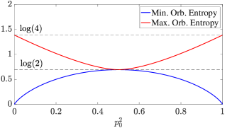
Figure 6: Minimal/maximal orbital entropy $S(\rho_{1/2})$ over all real orbital basis, against the amplitude $p_{0}^{2}$ in (31).

Third, maximal orbital entropy is achieved by a $\frac{\pi}{4}$-rotation from the reference orbitals. When $\theta=\frac{\pi}{4}$, the spectrum of the RDMs is given by

$$\begin{split}\mathrm{Spec}\left(\rho_{1/2}\left(\mathbf{p},\frac{\pi}{4}\right)\right)&=\left\{\left(\frac{p_{0}+p_{2}}{2}\right)^{2},\left(\frac{p_{0}-p_{2}}{2}\right)^{2},\right.\\ &\left.\quad\left(\frac{p_{0}-p_{2}}{2}\right)^{2},\left(\frac{p_{0}+p_{2}}{2}\right)^{2}\right\}.\end{split}$$ (36)

Notice that

$$\begin{split}\mathrm{Spec}(\rho_{1/2}(\mathbf{p},\theta))&\succ\left\{\frac{q_{0}(\theta)^{2}+q_{2}(\theta)}{2},\frac{q_{1}(\theta)^{2}}{2},\right.\\ &\quad\left.\frac{q_{1}(\theta)^{2}}{2},\frac{q_{0}(\theta)^{2}+q_{2}(\theta)}{2}\right\}\\ &\succ\mathrm{Spec}\left(\rho_{1/2}\left(\mathbf{p},\frac{\pi}{4}\right)\right).\end{split}$$ (37)

Therefore the orbital entropy is maximal when $\theta=\frac{\pi}{4}$, which equals to

$$\begin{split}S\left(\rho_{1/2}\left(\mathbf{p},\frac{\pi}{4}\right)\right)&=-2\left(\frac{p_{0}+p_{2}}{2}\right)^{2}\log\left[\left(\frac{p_{0}+p_{2}}{2}\right)^{2}\right]\\ &\quad-2\left(\frac{p_{0}-p_{2}}{2}\right)^{2}\log\left[\left(\frac{p_{0}-p_{2}}{2}\right)^{2}\right].\end{split}$$ (38)

To summarize, through orbital rotation, one can minimize/maximize the orbital entropy of the two-electron state, which in this case coincide with a measure of multireference character, namely the CI entropy. The orbital entropy is minimized when $|\Psi\rangle$ is expressed in a zero senority form, and is maximized when a $\frac{\pi}{4}$-rotation is applied to the minimizing orbital basis. These findings are encapsulated in Figure 6, where we presented the minimal/maximal single orbital entropy $S(\rho_{1/2})$ over all real orbital basis, against the amplitude $p_{0}^{2}$. When $p_{0}^{2}=0,1$, the state is a single Slater determinant, and correspondingly the minimal orbital entropy vanishes. As $p_{0}^{2}$ approaches $1/2$, $|\Psi\rangle$ becomes more multireference, and accordingly the minimal orbital entropy increases. When $p_{0}^{2}=1/2$, the two orbitals are equally correlated/entangled in every orbital basis. In other words, the complexity of the state cannot be transformed away by orbital rotation. In contrast, the maximal orbital entropy behaves in the opposite manner. It is maximal when $p_{0}^{2}=0,1$, and minimal when $p_{0}^{2}=1/2$. It signals the triviality of the orbital correlation of a single reference state in a poorly chosen orbital basis.

Figure 7: TCCSD-QIO optimization of the Cr₂ molecule at the bond length of 1.679 ${\rm\AA}$ in the cc-pV5Z-DK basis set, consisting of 306 orbitals. A minimal active space of (12,12) is used. The inset shows the details of the TCCSD energies and the total entanglement entropies as the orbitals are optimized.

Appendix C TCCSD-QIO optimization of Cr₂

In the original QICAS paper [73], a truncated set of orbitals were used due to the huge computational cost of low-bond DMRG calculation. We also point out that the CASSCF algorithm in this case also gets very expensive. As the optimization proceeds, the active space CASCI energies decrease and eventually converge slightly above the CASSCF energy, while the TCCSD energies decrease below the one using CASSCF canonical orbitals. The abrupt decrease in the TCCSD energy at iteration 1 results from the orbital rotation traversing a region where the reference determinant isn’t dominant, and the tailored MP2 (TMP2) ansatz is employed to navigate out of this region. Even at the equilibrium bond length, the wavefunction exhibits a large amount of multi-reference character, as indicated by the large reduction of roughly 700 mHa in the CASCI energy in the active space alone from the initial HF orbitals to the final QIO orbitals. The difference between the CASCI and TCCSD energies can be considered as the dynamical correlation energy, which is on the order of 1000 mHa across the optimization.

Appendix D Original Data

Table 1: TCCSD energy and entropy data for C₂ presented in Fig. 5 in the main text. Energy in Hartree.

C-C (Bohr)	QIO	TCCSD-NO	CASSCF-NO	UCCSD-NO	HFO	FQIO
1.8	-75.4537845	-75.4538515	-75.451787	-75.4505035	-75.4477625	2.775
2.0	-75.6339123	-75.6338969	-75.631530	-75.6304366	-75.6281571	2.987
2.2	-75.7105573	-75.7102883	-75.707881	-75.7067405	-75.7047199	3.190
2.4	-75.7284669	-75.7281048	-75.725810	-75.7244722	-75.7226391	3.384
2.6	-75.7151864	-75.7145051	-75.712407	-75.7108455	-75.7092274	3.575
2.8	-75.6858595	-75.6858930	-75.684042	-75.6823171	-75.6811697	3.634
3.0	-75.6522752	-75.6521957	-75.650593	-75.6487491	-75.6485821	3.725
3.2	-75.6342023	-75.6345553	-75.632930	-75.6334080	-75.6296234	2.466
3.4	-75.6143219	-75.6144370	-75.612805	-75.6131546	-75.6097061	2.607
3.6	-75.5952101	-75.5951644	-75.593422	-75.5935781	-75.5904149	2.764
3.8	-75.5779611	-75.5777775	-75.575879	-75.5757977	-75.5728311	2.937
4.0	-75.5630263	-75.5628871	-75.560785	-75.5604078	-75.5575338	3.133
4.2	-75.5508078	-75.5507175	-75.548390	-75.5477326	-75.5447838	3.361
4.4	-75.5412382	-75.5412656	-75.538661	-75.5378033	-75.5346044	3.628
4.6	-75.5340541	-75.5341825	-75.531360	-75.5304352	-75.5268035	3.922
4.8	-75.5288546	-75.5290184	-75.526062	-75.5251912	-75.5210413	4.220
5.0	-75.5250909	-75.5252870	-75.522268	-75.5215623	-75.5168579	4.496
5.2	-75.5223409	-75.5225585	-75.519520	-75.5190494	-75.5138422	4.732
5.4	-75.5202896	-75.5204730	-75.517464	-75.5172273	-75.5116615	4.925
5.6	-75.5186942	-75.5188673	-75.515894	-75.5158398	-75.5100565	5.077
5.8	-75.5174429	-75.5175640	-75.514640	-75.5147167	-75.5088626	5.196

Table 2: TCCSD energy and entropy data for Cr₂ presented in Fig. 5 in the main text. Energy in Hartree.

Cr-Cr ($\AA$)	QIO	TCCSD-NO	CASSCF-NO	UCCSD-NO	FQIO
1.50	-2099.8682088	-2099.8665733	-2099.8604731	-2099.8505611	5.869
1.55	-2099.8805779	-2099.8790180	-2099.8715983	-2099.8594378	6.159
1.57	N/A	N/A	-2099.8741577	-2099.8609289	N/A
1.60	-2099.8869346	-2099.8855955	-2099.8765241	-2099.8614968	6.514
1.64	-2099.8895896	-2099.8882957	-2099.8777240	-2099.8598751	6.853
1.68	-2099.8907057	-2099.8896679	-2099.8774932	-2099.8564156	7.226
1.73	-2099.8910933	-2099.8903517	-2099.8761989	-2099.8506864	7.719
1.80	-2099.8908079	-2099.8903717	-2099.8735534	-2099.8422357	8.386
1.90	-2099.8897337	N/A	-2099.8690127	-2099.8338818	9.175
2.00	N/A	N/A	-2099.8633707	-2099.8345337	N/A

References

- Sharma et al. [2014] S. Sharma, K. Sivalingam, F. Neese, and G. K.-L. Chan, Nature Chemistry 6, 927 (2014).
- Kurashige et al. [2013] Y. Kurashige, G. K.-L. Chan, and T. Yanai, Nature Chemistry 5, 660 (2013).
- Booth et al. [2013] G. H. Booth, A. Grüneis, G. Kresse, and A. Alavi, Nature 493, 365 (2013), 23254929 .
- Bogdanov et al. [2022] N. A. Bogdanov, G. Li Manni, S. Sharma, O. Gunnarsson, and A. Alavi, Nature Physics 18, 190 (2022).
- Cui et al. [2022] Z.-H. Cui, H. Zhai, X. Zhang, and G. K.-L. Chan, Science 377, 1192 (2022).
- Kato [1957] T. Kato, Communications on Pure and Applied Mathematics 10, 151 (1957).
- Shepherd and Grüneis [2013] J. J. Shepherd and A. Grüneis, Physical Review Letters 110, 10.1103/PhysRevLett.110.226401 (2013), arxiv:1310.6059 .
- Ochi et al. [2017] M. Ochi, R. Arita, and S. Tsuneyuki, Physical Review Letters 118, 026402 (2017).
- Masios et al. [2023] N. Masios, A. Irmler, T. Schäfer, and A. Grüneis, Physical Review Letters 131, 186401 (2023).
- Neufeld and Berkelbach [2023] V. A. Neufeld and T. C. Berkelbach, Physical Review Letters 131, 186402 (2023).
- Drummond and Needs [2007] N. D. Drummond and R. J. Needs, Physical Review Letters 99, 166401 (2007).
- Tkatchenko et al. [2012] A. Tkatchenko, R. A. DiStasio, R. Car, and M. Scheffler, Physical Review Letters 108, 236402 (2012).
- Cioslowski et al. [2023] J. Cioslowski, C. Schilling, and R. Schilling, The Journal of Chemical Physics 158, 084106 (2023).
- Schollwöck [2005] U. Schollwöck, Reviews of Modern Physics 77, 259 (2005).
- Chan and Sharma [2011] G. K.-L. Chan and S. Sharma, Annual Review of Physical Chemistry 62, 465 (2011).
- Baiardi and Reiher [2020] A. Baiardi and M. Reiher, The Journal of Chemical Physics 152, 040903 (2020).
- Booth et al. [2009] G. H. Booth, A. J. Thom, and A. Alavi, Journal of Chemical Physics 131, 054106 (2009).
- Cleland et al. [2010] D. Cleland, G. H. Booth, and A. Alavi, Journal of Chemical Physics 132, 10.1063/1.3302277 (2010).
- Li Manni et al. [2016] G. Li Manni, S. D. Smart, and A. Alavi, Journal of Chemical Theory and Computation 12, 1245 (2016).
- Shi and Zhang [2021] H. Shi and S. Zhang, The Journal of Chemical Physics 154, 024107 (2021).
- Lee et al. [2022] J. Lee, H. Q. Pham, and D. R. Reichman, Journal of Chemical Theory and Computation 18, 7024 (2022).
- Andersson et al. [1992] K. Andersson, P.-Å. Malmqvist, and B. O. Roos, The Journal of Chemical Physics 96, 1218 (1992).
- Angeli et al. [2001] C. Angeli, R. Cimiraglia, S. Evangelisti, T. Leininger, and J.-P. Malrieu, The Journal of Chemical Physics 114, 10252 (2001).
- Li Manni et al. [2014] G. Li Manni, R. K. Carlson, S. Luo, D. Ma, J. Olsen, D. G. Truhlar, and L. Gagliardi, Journal of Chemical Theory and Computation 10, 3669 (2014).
- Gagliardi et al. [2017] L. Gagliardi, D. G. Truhlar, G. Li Manni, R. K. Carlson, C. E. Hoyer, and J. L. Bao, Accounts of Chemical Research 50, 66 (2017).
- Bartlett and Musiał [2007] R. Bartlett and M. Musiał, Reviews of Modern Physics 79, 291 (2007).
- Kats and Manby [2013] D. Kats and F. R. Manby, The Journal of Chemical Physics 139, 021102 (2013).
- Kats [2014] D. Kats, The Journal of Chemical Physics 141, 061101 (2014).
- Gruber et al. [2018] T. Gruber, K. Liao, T. Tsatsoulis, F. Hummel, and A. Grüneis, Physical Review X 8, 21043 (2018).
- Kats and Köhn [2019] D. Kats and A. Köhn, The Journal of Chemical Physics 150 (2019).
- Yang et al. [2000] W. Yang, Y. Zhang, and P. W. Ayers, Physical Review Letters 84, 5172 (2000).
- Mazziotti [2006] D. A. Mazziotti, Physical Review Letters 97, 143002 (2006).
- Mazziotti [2008] D. A. Mazziotti, Physical Review Letters 101, 253002 (2008).
- Schilling and Pittalis [2021] C. Schilling and S. Pittalis, Physical Review Letters 127, 023001 (2021).
- Neuscamman et al. [2010] E. Neuscamman, T. Yanai, and G. K.-L. Chan, International Reviews in Physical Chemistry 29, 231 (2010).
- Luo and Alavi [2018] H. Luo and A. Alavi, Journal of Chemical Theory and Computation 14, 1403 (2018).
- Vitale et al. [2020] E. Vitale, A. Alavi, and D. Kats, Journal of Chemical Theory and Computation 16, 5621 (2020).
- Liao et al. [2021] K. Liao, T. Schraivogel, H. Luo, D. Kats, and A. Alavi, Physical Review Research 3, 033072 (2021).
- Schraivogel et al. [2021] T. Schraivogel, A. J. Cohen, A. Alavi, and D. Kats, The Journal of Chemical Physics 155, 191101 (2021).
- Baiardi et al. [2022] A. Baiardi, M. Lesiuk, and M. Reiher, Journal of Chemical Theory and Computation 18, 4203 (2022).
- Liao et al. [2023] K. Liao, H. Zhai, E. M. Christlmaier, T. Schraivogel, P. L. Ríos, D. Kats, and A. Alavi, Journal of Chemical Theory and Computation 19, 1734 (2023).
- Löwdin [1955] P.-O. Löwdin, Physical Review 97, 1474 (1955).
- Taube and Bartlett [2005] A. G. Taube and R. J. Bartlett, Collection of Czechoslovak Chemical Communications 70, 837 (2005).
- Taube and Bartlett [2008] A. G. Taube and R. J. Bartlett, The Journal of Chemical Physics 128, 164101 (2008).
- Grüneis et al. [2011] A. Grüneis, G. H. Booth, M. Marsman, J. Spencer, A. Alavi, and G. Kresse, Journal of Chemical Theory and Computation 7, 2780 (2011).
- Liao et al. [2019] K. Liao, X.-Z. Li, A. Alavi, and A. Grüneis, npj Computational Materials 5, 1 (2019).
- Kong et al. [2012] L. Kong, F. A. Bischoff, and E. F. Valeev, Chemical Reviews 112, 75 (2012).
- Ma et al. [2017] Q. Ma, M. Schwilk, C. Köppl, and H.-J. Werner, Journal of Chemical Theory and Computation 13, 4871 (2017).
- Pavošević et al. [2017] F. Pavošević, C. Peng, P. Pinski, C. Riplinger, F. Neese, and E. F. Valeev, The Journal of Chemical Physics 146, 174108 (2017).
- Kállay et al. [2023] M. Kállay, R. A. Horváth, L. Gyevi-Nagy, and P. R. Nagy, Journal of Chemical Theory and Computation 19, 174 (2023).
- Dobrautz et al. [2023] W. Dobrautz, I. O. Sokolov, K. Liao, P. L. Ríos, M. Rahm, A. Alavi, and I. Tavernelli, Ab Initio Transcorrelated Method enabling accurate Quantum Chemistry on near-term Quantum Hardware (2023), arxiv:2303.02007 [cond-mat, physics:physics, physics:quant-ph] .
- Li et al. [2009] W. Li, P. Piecuch, J. R. Gour, and S. Li, The Journal of Chemical Physics 131, 114109 (2009).
- Rolik et al. [2013] Z. Rolik, L. Szegedy, I. Ladjánszki, B. Ladóczki, and M. Kállay, The Journal of Chemical Physics 139, 094105 (2013).
- Srednicki [1993] M. Srednicki, Physical Review Letters 71, 666 (1993).
- Hastings [2007] M. B. Hastings, Physical Review B 76, 035114 (2007).
- Eisert et al. [2010] J. Eisert, M. Cramer, and M. B. Plenio, Reviews of Modern Physics 82, 277 (2010).
- Krumnow et al. [2016] C. Krumnow, L. Veis, Ö. Legeza, and J. Eisert, Physical Review Letters 117, 210402 (2016), arxiv:1504.00042 [cond-mat, physics:physics, physics:quant-ph] .
- Li Manni et al. [2020] G. Li Manni, W. Dobrautz, and A. Alavi, Journal of Chemical Theory and Computation 16, 2202 (2020).
- Roos [1980] B. O. Roos, International Journal of Quantum Chemistry 18, 175 (1980).
- Siegbahn et al. [1981] P. E. M. Siegbahn, J. Almlöf, A. Heiberg, and B. O. Roos, The Journal of Chemical Physics 74, 2384 (1981).
- Larsson et al. [2022] H. R. Larsson, H. Zhai, C. J. Umrigar, and G. K.-L. Chan, Journal of the American Chemical Society 144, 15932 (2022).
- Tóth and Pulay [2020] Z. Tóth and P. Pulay, Journal of Chemical Theory and Computation 16, 7328 (2020).
- Note [1] The selection of the active space in general is a very challenging task on its own, here we focus on the optimization of the orbitals within a given active space size.
- Lee and Head-Gordon [2018] J. Lee and M. Head-Gordon, Journal of Chemical Theory and Computation 14, 5203 (2018).
- Boguslawski et al. [2012] K. Boguslawski, P. Tecmer, Ö. Legeza, and M. Reiher, The Journal of Physical Chemistry Letters 3, 3129 (2012).
- Boguslawski and Tecmer [2015] K. Boguslawski and P. Tecmer, International Journal of Quantum Chemistry 115, 1289 (2015).
- Stein and Reiher [2016] C. J. Stein and M. Reiher, Journal of Chemical Theory and Computation 12, 1760 (2016).
- Stein and Reiher [2017] C. J. Stein and M. Reiher, Molecular Physics 115, 2110 (2017).
- Ding and Schilling [2020] L. Ding and C. Schilling, Journal of Chemical Theory and Computation 16, 4159 (2020).
- Ding et al. [2021] L. Ding, S. Mardazad, S. Das, S. Szalay, U. Schollwöck, Z. Zimborás, and C. Schilling, Journal of Chemical Theory and Computation 17, 79 (2021).
- Henderson and Vedral [2001] L. Henderson and V. Vedral, Journal of Physics A: Mathematical and General 34, 6899 (2001).
- Groisman et al. [2005] B. Groisman, S. Popescu, and A. Winter, Physical Review A 72, 032317 (2005).
- Ding et al. [2023] L. Ding, S. Knecht, and C. Schilling, The Journal of Physical Chemistry Letters 14, 11022 (2023).
- Modi et al. [2010] K. Modi, T. Paterek, W. Son, V. Vedral, and M. Williamson, Physical Review Letters 104, 080501 (2010).
- Gigena and Rossignoli [2015] N. Gigena and R. Rossignoli, Physical Review A 92, 042326 (2015).
- Kinoshita et al. [2005] T. Kinoshita, O. Hino, and R. J. Bartlett, The Journal of Chemical Physics 123, 074106 (2005).
- Zhai et al. [2023] H. Zhai, H. R. Larsson, S. Lee, Z.-H. Cui, T. Zhu, C. Sun, L. Peng, R. Peng, K. Liao, J. Tölle, J. Yang, S. Li, and G. K.-L. Chan, The Journal of Chemical Physics 159, 234801 (2023).
- Wouters et al. [2014] S. Wouters, W. Poelmans, P. W. Ayers, and D. Van Neck, Computer Physics Communications 185, 1501 (2014).
- Kutzelnigg and Liu [2005] W. Kutzelnigg and W. Liu, The Journal of Chemical Physics 123, 241102 (2005).
- Peng and Reiher [2012] D. Peng and M. Reiher, Theoretical Chemistry Accounts 131, 1081 (2012).
- Sun et al. [2020] Q. Sun, X. Zhang, S. Banerjee, P. Bao, M. Barbry, N. S. Blunt, N. A. Bogdanov, G. H. Booth, J. Chen, Z.-H. Cui, J. J. Eriksen, Y. Gao, S. Guo, J. Hermann, M. R. Hermes, K. Koh, P. Koval, S. Lehtola, Z. Li, J. Liu, N. Mardirossian, J. D. McClain, M. Motta, B. Mussard, H. Q. Pham, A. Pulkin, W. Purwanto, P. J. Robinson, E. Ronca, E. R. Sayfutyarova, M. Scheurer, H. F. Schurkus, J. E. T. Smith, C. Sun, S.-N. Sun, S. Upadhyay, L. K. Wagner, X. Wang, A. White, J. D. Whitfield, M. J. Williamson, S. Wouters, J. Yang, J. M. Yu, T. Zhu, T. C. Berkelbach, S. Sharma, A. Y. Sokolov, and G. K.-L. Chan, The Journal of Chemical Physics 153, 024109 (2020).
- Roos [2003] B. O. Roos, Collection of Czechoslovak Chemical Communications 68, 265 (2003).
- Kurashige and Yanai [2011] Y. Kurashige and T. Yanai, The Journal of Chemical Physics 135, 094104 (2011).
- Hongo and Maezono [2012] K. Hongo and R. Maezono, International Journal of Quantum Chemistry 112, 1243 (2012).
- Li Manni et al. [2013] G. Li Manni, D. Ma, F. Aquilante, J. Olsen, and L. Gagliardi, Journal of Chemical Theory and Computation 9, 3375 (2013).
- Yamada et al. [2013] Y. Yamada, K. Hongo, K. Egashira, Y. Kita, U. Nagashima, and M. Tachikawa, Chemical Physics Letters 555, 84 (2013).
- Purwanto et al. [2015] W. Purwanto, S. Zhang, and H. Krakauer, The Journal of Chemical Physics 142, 064302 (2015).
- Vancoillie et al. [2016] S. Vancoillie, P. Å. Malmqvist, and V. Veryazov, Journal of Chemical Theory and Computation 12, 1647 (2016).
- Leszczyk et al. [2022] A. Leszczyk, M. Máté, Ö. Legeza, and K. Boguslawski, Journal of Chemical Theory and Computation 18, 96 (2022).
- Veis et al. [2016] L. Veis, A. Antalík, J. Brabec, F. Neese, Ö. Legeza, and J. Pittner, The Journal of Physical Chemistry Letters 7, 4072 (2016).