Training Neural Networks from Scratch with Parallel Low-Rank Adapters

Abstract

The scalability of deep learning models is fundamentally limited by computing resources, memory, and communication. Although methods like low-rank adaptation (LoRA) have reduced the cost of model finetuning, its application in model pre-training remains largely unexplored. This paper explores extending LoRA to model pre-training, identifying the inherent constraints and limitations of standard LoRA in this context. We introduce LoRA-the-Explorer (LTE), a novel bi-level optimization algorithm designed to enable parallel training of multiple low-rank heads across computing nodes, thereby reducing the need for frequent synchronization. Our approach includes extensive experimentation on vision transformers using various vision datasets, demonstrating that LTE is competitive with standard pre-training.
$\triangleright\;\mathsf{project\;page}:$ minyoungg.github.io/LTE

1 Introduction

The escalating complexity of state-of-the-art deep learning models presents significant challenges not only in terms of computational demand but also in terms of memory and communication bandwidth. As these demands exceed the capacity of consumer-grade GPUs, training larger models requires innovative solutions. A prominent example for finetuning models is low-rank adaptation (Hu et al., 2022) that uses a low-rank parameterization of a deep neural network to reduce memory requirements for storing optimizer-state and gradient communication during training. The memory requirement was further reduced by quantizing model parameters (Dettmers et al., 2023). Such innovations have enabled the finetuning of large models, even on a single consumer-grade GPU.

However, prior work has been limited to finetuning, and tools to pre-train models from scratch are still absent. Hence, the goal of this paper is to extend adaptation methods to model pre-training. Specifically, we ask the question: Can neural networks be trained from scratch using low-rank adapters?

Successfully addressing this question carries substantial implications, especially considering that common computing clusters often have slower cross-node training than single-node training with gradient accumulation due to slow communication speed and bandwidth. Low-rank adapters effectively compress the communication between these processors while preserving essential structural attributes for effective model training. Our investigation reveals that while vanilla LoRA underperforms in training a model from scratch, the use of parallel low-rank updates can bridge this performance gap.

Figure 1: Lora-The-Explorer: We propose LoRA-the-explorer, an optimization algorithm that can match the performance of standard training from scratch. Our method optimizes unique LoRA parameters in parallel and merges them back to the main weights. Our algorithm can leverage lower-memory devices and only depends on communicating the LoRA parameters for training, making it an ideal candidate in a bandlimited or memory-constraint training framework.

Principal findings and contributions:

• In Section 3, we establish limitations inherent to LoRA for model pre-training. We show that parallel updates are needed and introduce our algorithmic approach LTE in Section 3.1 and Section 3.3.

• In Section 4 we combine LTE with federated averaging (McMahan et al., 2017), to demonstrate comparable performance to distributed pre-training, even with infrequent synchronization.

• We provide empirical analysis and ablation studies in Section 4.1, Section 4.2, and Section 4.3.

• In Section 4.5, we conduct a resource utilization comparison with standard distributed data-parallel (DDP) training on $8$ GPUs. Although our method extends the training samples required for convergence by $40\%$, we can fit models that are $3\times$ bigger with roughly half the bandwidth. This, in turn, enables faster training if one has access to many low-memory devices.

Differences to existing works

Our work explores a new territory in the pre-training paradigm, leveraging both data and model parallelism. Our approach stores different copies of the LoRA parameters and is trained on different shards of the data distribution. This is in contrast with traditional federated learning, which replicates the same model across devices, and in-silo distributed training, which either divides the model across many devices for model parallelism or replicates the exact same model across devices for data parallelism. Our method enables distributed training with infrequent synchronizations while allowing for single-device inference. Several concurrent works have aimed at similar goals. We highlight a few notable works below:

ReLoRA (Lialin et al., 2023) sequentially trains and merges LoRA parameters back into the main weights. However, it does not yield comparable pre-training performance without initial full-parameter training. In contrast, our work uses parallel updates to match pre-training performance without bells and whistles.

FedLoRA (Yi et al., 2023) is designed to train LoRA parameters for finetuning within a federated learning framework. It involves training multiple LoRAs and averaging them into a single global LoRA. FedLoRA focuses on the distributed finetuning of LoRA parameters.

AdaMix (Wang et al., 2022) averages all MLPs in a Mixture of Experts (MOE) into a single MLP. AdaMix requires constant synchronization during the forward and backward passes. Our work requires no synchronization in the forward pass, and merging of the parameters can happen infrequently.

For an in-depth discussion of related works, see Section 5.

2 Preliminaries

Unless stated otherwise, we denote $x$ as a scalar, $\mathbf{x}$ a vector, $\mathbf{X}$ a matrix, $\mathcal{X}$ a distribution or a set, $f(\cdot)$ a function and $F(\cdot)$ a composition of functions, and $\mathcal{L}(\cdot,\cdot)$ a loss-function.

2.1 Parameter efficient adapters

Adapters serve as trainable functions that modify existing layers in a neural network. They facilitate parameter-efficient finetuning of large-scale models by minimizing the memory requirements for optimization (see Section 5 for various types of adapters used in prior works).

The focus of this work is on the low-rank adapter (Hu et al., 2022, LoRA), a subclass of linear adapters. The linearity of LoRA allows for the trained parameters to be integrated back into the existing weights post-training without further tuning or approximation. Hence, the linearity allows models to maintain the original inference cost. LoRA is frequently used for finetuning transformers, often resulting in less than $10\%$ of the total trainable parameters (even as low as $0.5\%$).

Low-Rank Adapter (LoRA)   Given input $\mathbf{x}\in\mathbb{R}^{n}$, and a linear layer $f(\cdot):\mathbb{R}^{n}\rightarrow\mathbb{R}^{m}$ parameterized by the weight $\mathbf{W}\in\mathbb{R}^{m\times n}$, LoRA re-parameterizes the function as:

$$f_{\mathsf{lora}}(\mathbf{x})=\mathbf{W}\mathbf{x}+s\mathbf{B}\mathbf{A}\mathbf{x}$$ (1)

For some low-rank matrices $\mathbf{B}\in\mathbb{R}^{m\times r}$, $\mathbf{A}\in\mathbb{R}^{r\times n}$ and a fixed scalar $s\in\mathbb{R}$, where the rank $r$ is often chosen such that $r\ll\min(m,n)$.

Although the forward pass incurs an extra computational overhead, the significance of LoRA parameterization pertains to the optimizer memory footprint. Optimizers such as AdamW (Kingma & Ba, 2015; Loshchilov & Hutter, 2019) typically maintain two states for each parameter, resulting in memory consumption that is twice the size of the trainable parameters. In the case of LoRA parameterization, the optimizer memory scales with the combined sizes of $\mathbf{A}$ and $\mathbf{B}$. This results in significant memory savings when the memory cost of LoRA $\mathcal{O}(r(m+n))$ is less than the memory cost of the model $\mathcal{O}(mn)$. Moreover, QLoRA (Dettmers et al., 2023) achieves further memory savings by storing $\mathbf{W}$ in low-precision (4bit) while keeping the trainable parameters $\mathbf{A}$ and $\mathbf{B}$ in higher-precision (16bit). These works have catalyzed the development of several repositories (Wang, 2023; Dettmers et al., 2023; Dettmers, 2023; huggingface, 2023), enabling finetuning of models with billions of parameters on low-memory devices.

3 Method

To understand the conditions required to pre-train a model with LoRA, we first identify a specific scenario where standard training performance can be recovered using LoRA. This serves as a guide for developing our algorithm that retains the memory efficiency of LoRA.

Although low-rank adapters (LoRAs) have proven to be an effective finetuning method, they have apparent limitations when pre-training. As evidenced in Figure 2, models parameterized with LoRA demonstrate inferior performance compared to models trained using standard optimization. This performance gap isn’t surprising as it can be attributed to the inherent rank constraint in LoRA. Specifically, for parameter $\mathbf{W}\in\mathbb{R}^{m\times n}$, LoRA is fundamentally incapable of recovering weights that exceed the rank $r<\min(m,n)$. Of course, there are exceptions in which, by happenstance, a solution exists within a low-rank proximity of the initialization. However, in Appendix B, we observed the rank of the gradient tends to increase throughout training, hinting at the necessity for high-rank updates.

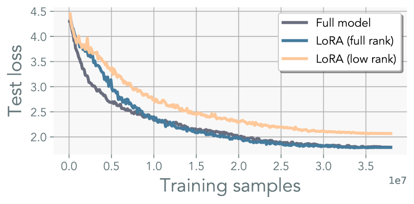
Figure 2: Increasing the rank of LoRA can recover the standard training performance: ViT-S trained on ImageNet100 using with and without LoRA. Low-rank LoRA uses rank $r=64$, and full-rank LoRA uses rank $r=\min(m,n)$ set to the dimension of the original weight $\mathbf{W}\in\mathbb{R}^{m\times n}$. Increasing $r$ suffices to match standard training performance.

3.1 Motivation: Multi-head merging perspective

This section provides intuition on why LoRA heads in parallel can achieve the performance of standard pre-training.

As demonstrated in Figure 2, elevating the rank $r$ of the LoRA to be the same as the rank $\min(m,n)$ of the weight matrix $\mathbf{W}\in\mathbb{R}^{m\times n}$ is sufficient to replicate standard pre-training performance, albeit with different inherent dynamics as detailed in Appendix B.2. However, such an approach compromises the memory efficiency of low-rank adapters.

Therefore, we investigate the possibility of arriving at an equivalent performance by leveraging multiple low-rank adapters in parallel. Our motivation leverages the trivial idea of linearity of these adapters to induce parallelization.

Given a matrix of the form $\mathbf{B}\mathbf{A}\in\mathbb{R}^{d_{1}\times d_{2}}$ with $\mathbf{B}\in\mathbb{R}^{d_{1}\times d}$ and $\mathbf{A}\in\mathbb{R}^{d\times d_{2}}$, it is possible to represent the product as the sum of two lower-rank matrices: $\mathbf{B}_{1}\mathbf{A}_{1}+\mathbf{B}_{2}\mathbf{A}_{2}$. To demonstrate this, let $\mathbf{b}_{i}$ and $\mathbf{a}_{i}$ be the column vectors of $\mathbf{B}$ and $\mathbf{A}$ respectively. One can then construct $\mathbf{B}_{1}=[\mathbf{b}_{1},\dots,\mathbf{b}_{[d/2]}]$ , $\mathbf{B}_{2}=[\mathbf{b}_{[d/2]},\dots,\mathbf{b}_{d}]$, and $\mathbf{A}_{1}=[\mathbf{a}_{1}^{T},\dots,\mathbf{a}_{[d/2]}^{T}]$ , $\mathbf{A}_{2}=[\mathbf{a}_{[d/2]}^{T},\dots,\mathbf{a}_{d}^{T}]$. This decomposition allows for the approximation of high-rank matrices through a linear combination of lower-rank matrices. The same conclusion can be reached by beginning with a linear combination of rank-1 matrices. This forms the basis for a novel multi-head LoRA parameterization, which we will use as one of the baselines to compare with our final method.

Multi-head LoRA (MHLoRA)   Given a matrix $\mathbf{W}\in\mathbb{R}^{m\times n}$, and constant $N$, multi-head LoRA parameterizes the weights as a linear combination of $N$ low-rank matrices $\mathbf{B}_{n}$ and $\mathbf{A}_{n}$:

$$f_{\mathsf{mhlora}}(\mathbf{x})=\mathbf{W}\mathbf{x}+\frac{s}{N}\sum_{n=1}^{N}\mathbf{B}_{n}\mathbf{A}_{n}\mathbf{x}$$ (2)

Multi-head LoRA reparameterizes the full-rank weights into a linear combination of low-rank weights.

Now, we will point out a trivial observation that a single parallel LoRA head can approximate the trajectory of a single step of the multi-head LoRA, provided that the parallel LoRA heads are periodically merged into the full weights.

Using the same rank $r$ for all the LoRA parameters, the dynamics of a single parallel LoRA head (denoted with $\hat{\cdot}$ ) is equivalent to multi-head LoRA:

$$\operatorname*{arg\,min}_{\mathbf{B}_{n}\mathbf{A}_{n}}\mathcal{L} \left(\mathbf{W}+\frac{s}{N}\sum_{n=1}^{N}\mathbf{B}_{n}\mathbf{A}_{n}\right)$$

$$=\operatorname*{arg\,min}_{\hat{\mathbf{B}}_{n},\hat{\mathbf{A}}_{n}}\mathcal{L}\left(\hat{\mathbf{W}}+\frac{s}{N}\hat{\mathbf{B}}_{n}\hat{\mathbf{A}}_{n}\right)$$ (3)

When either $\sum_{n=1}^{N}\mathbf{B}_{n}\mathbf{A}_{n}$ is equal to $\hat{\mathbf{B}}_{n}\hat{\mathbf{A}}_{n}$, or when $\hat{\mathbf{W}}=\mathbf{W}+\frac{s}{N}\sum_{j\neq n}^{N}\mathbf{B}_{j}\mathbf{A}_{j}$; here we used a shorthand notation to indicate that sum is over all the LoRA parameters except for index $n$. We assume the parameters on both sides of the equation are initialized to be the same: $\mathbf{A}_{n}=\hat{\mathbf{A}}_{n}$ and $\mathbf{B}_{n}=\hat{\mathbf{B}}_{n}\forall n$. The first scenario is rank deficient, which we know is unable to recover the original model performance. The latter case necessitates that $\hat{\mathbf{W}}$ accumulates all the information of the LoRA parameters at every iteration. Hence, if we can apply a merge operator at every iteration, we can recover the exact update.

This rather simple observation implies that one can recover the exact gradient updates of the multi-head LoRA parameterized model, which we observed to match pre-training performance across a wide range of tasks (see Appendix D). Moreover, in a distributed setting, only the LoRA parameters/gradients have to be communicated across devices, which is often a fraction of the original model size, making it a good candidate where interconnect speed between computing nodes is limited.

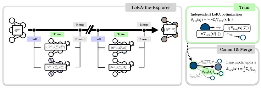
Figure 3: LTE diagram: Our method is decomposed into 3 steps. (1) We parameterize the model with multiple LoRA heads and train them independently for $T$ iterations using different mini-batches sampled from the same (homogeneous) distribution. This results in overall update of $\delta_{\mathsf{lora}_{n}}(\mathbf{x})=-\eta\sum_{t}\nabla_{\mathsf{lora}_{n}}(\mathbf{x}[t])$ (2). Next, we accumulate the individual LoRA updates by averaging the heads $\Delta_{\mathsf{lora}}(\mathbf{x})=\frac{1}{N}\sum_{n}\delta_{\mathsf{lora}_{n}}(\mathbf{x})$. (3) The update is applied to the main weights, and the LoRA parameter $\mathbf{B}$ is reset. The optimization repeats with the new LoRA parameters.

3.2 LoRA soup: delayed LoRA merging

To further reduce the communication cost of LTE, we extend and combine the ideas of local updates (McMahan et al., 2017) and model-averaging (Wortsman et al., 2022; Yadav et al., 2023; Ilharco et al., 2023). Instead of merging every iteration, we allow the LoRA parameters to train independently of each other for a longer period before the merge operator. This is equivalent to using stale estimates of the LoRA parameters $\hat{\mathbf{W}}=\mathbf{W}+\frac{s}{N}\sum_{j\neq n}^{N}\mathbf{B}_{j}^{\prime}\mathbf{A}_{j}^{\prime}$ with ^′ indicating a stale estimate of the parameters.

Merging every iteration ensures that the representation will not diverge from the intended update. While using stale estimates relaxes this equivalence, we observe that it can still match the standard training performance as shown in Table 1. Nevertheless, as the estimate becomes inaccurate, the optimization trajectory does indeed diverge from the optimization path of multi-head LoRA. We quantify this divergence in Figure LABEL:fig:lora-divergence. The divergence does not imply that the model won’t optimize; rather, it suggests that the optimization trajectory will deviate from that of the multi-head LoRA. In this work, we opt for simple averaging and leave more sophisticated merging such as those used in (Karimireddy et al., 2020; Matena & Raffel, 2022; Yadav et al., 2023) for future works.

3.3 LoRA-the-Explorer: parallel low-rank updates

Our algorithm is designed with two primary considerations: (1) achieving an informative update $\Delta\mathbf{W}$ that does not require materialization of the full parameter size during training, and (2) parameterizing $\mathbf{W}$ such that it can be stored in low-precision and communicated efficiently. The latter can be achieved by using quantized weights and keeping a high-precision copy of $\mathbf{W}$.

We propose LoRA-the-Explorer (LTE), an optimization algorithm that approximates full-rank updates with parallel low-rank updates. The algorithm creates $N$-different LoRA parameters for each linear layer at initialization. Each worker is assigned the LoRA parameter and creates a local optimizer. Next, the data is independently sampled from the same distribution $\mathbf{x}=\{\mathbf{x}_{1},\dots\mathbf{x}_{N}\}$. For each LoRA head $n$, the parameters are optimized with respect to its own data partition for $T$ iterations resulting in an update $\delta_{\mathsf{lora_{n}}}=-\eta\sum_{t=1}^{T}\nabla_{\mathsf{lora}_{n}}\mathbf{x}_{i}[t]$. We do not synchronize the optimizer state across workers. After the optimization, the resulting LoRA parameters are synchronized to compute the final update for the main weight $\Delta_{\mathsf{lora}}(\mathbf{x})=\frac{1}{N}\sum_{n=1}^{N}\delta_{n}$. In the next training cycle, the LoRA parameters are trained with the updated weights $\mathbf{W}$. Here, the LoRA parameters can be either be re-initialized or the same parameters can be used with the correction term (see Appendix A.2). Since we do not train directly on the main parameter $\mathbf{W}$, we can use the quantized parameter $q(\mathbf{W})$ instead. Where one can either keep the high-precision weight only in the master node or offload it from the device during training. This reduces not only the memory footprint of each worker but also the transmission overhead. A pseudo-code is provided in Algorithm 1 and an illustration in Figure 3.

3.4 Implementation details

We discuss a few of the implementation details we found necessary for improving the convergence speed and the performance of our method. Full training details and the supporting experiments can be found in Appendix A.

Not resetting matrix $\mathbf{A}$ and optimizer states   We investigate whether the matrices $\mathbf{A}_{n}$ would converge to the same sub-space during training. If so, it would necessitate resetting of matrices $\mathbf{A}_{n}$ or the use of a regularizer. In Figure 8, we did not observe this to be the case. We observed the orthogonality of $\mathbf{A}$ to remain consistent throughout training, and we found it to perform better without resets. We posit that re-learning matrix $\mathbf{A}$ and re-accumulating the optimizer state ends up wasting optimization steps. The comparison figures can be found in Appendix A.4 and a more detailed discussion in Section 4.2.

Scaling up $s$ and lowering learning rate $\eta$

It is a common misconception that scaling $s$ has the same effect as tuning the learning rate $\eta$. During our experimentation, we were unable to yield comparable performance when using the standard value of $s$ (in the range of $1\sim 4$). Instead, we found using a large value of $s$ and a slightly lower learning rate $\eta$ to work the best. The standard practice is to set the scaling proportionately to the rank of the LoRA $s=\alpha/r$. This is done to automatically adjust for the rank (Hu et al., 2022). We use $\alpha=4096$ ($s=64$) and a learning rate of $\eta=2\cdot 10^{-4}$. It is worth noting that the learning rate does not scale linearly with $s$, and the scalar only affects the forward computation (Appendix B.1). The scalar $s$ modifies the contribution of the LoRA parameters in the forward pass which has a non-trivial implication on the effective gradient. Moreover, in Appendix B.2, we provide the effective update rule of LoRA updates and observe the emergence of the term $s$ that scales quadratically with the alignment of $\mathbf{B}$ and $\mathbf{A}$. Since $s$ is large relative to the learning rate, it may have a non-negligible effect on the dynamics.

Input: Dataset $\mathcal{D}_{\mathsf{train}}$, model $\mathcal{F}$, loss function $\mathcal{L}$

    parameters $\Theta=\{\mathbf{W}_{0},\dots,\mathbf{W}_{L}\}$,

    merge scalar $s$, num workers $N$, merge iter $T$

 

while not converged do

       (Optional) quantize $\Theta$. Keep high-precision copy

       (in parallel) for each worker $n$ do

             if LoRA not initialized then

                   $\mathcal{B}_{n},\mathcal{A}_{n}\leftarrow\mathbf{lora\_parameterize}(\mathcal{F})$

                  

            else

                   (Optional) reset parameters $\mathcal{B}_{n}$ to zero

                  

            Optimize $\mathcal{B}_{n},\mathcal{A}_{n}$ for $T$ iterations by minimizing $\mathbb{E}_{\mathbf{x},\mathbf{y}\sim\mathcal{D}_{\mathsf{train}}}\left[\mathcal{L}(\mathcal{F}(\mathbf{x}),\mathbf{y})\right]$

            

      

       # Synchronize by communicating LoRA parameters.

       for each worker $n$ do

             for $\mathbf{B}_{n},\mathbf{A}_{n}$ in $\mathcal{B}_{n},\mathcal{A}_{n}$ do

                   Merge LoRA params $\mathbf{W}_{n}\leftarrow\mathbf{W}_{n}+\frac{s}{n}\mathbf{B}_{n}\mathbf{A}_{n}$

                  

Algorithm 1 LoRA-the-Explorer (LTE)

Figure 5: LTE pseudocode. Not resetting $\mathcal{B}_{n}$ requires a correction term to LTE. See Appendix A.2.

Significance of Initialization Strategies

Initialization of LoRA plays a pivotal role in pre-training. Kaiming initialization used in the original work (Hu et al., 2022) – are not well-suited for rectangular matrices as discussed in (Bernstein et al., 2023; Yang et al., 2024a). Given that LoRA parameterization often leads to wide matrices, alternative methods from (Bernstein et al., 2023) and (Glorot & Bengio, 2010) resulted in better empirical performance.

We use the initialization scheme prescribed in (Bernstein et al., 2023) that utilizes a semi-orthogonal matrix scaled by $\sqrt{d_{out}/d_{in}}$. Note that these methods were originally designed for standard feed-forward models. Whereas LoRA operates under the assumption that matrix $\mathbf{B}$ is zero-initialized with a residual connection. This aspect warrants further study for exact gain calculations. Our ablation studies, in Appendix A.4, indicate the best performance with (Bernstein et al., 2023), with Kaiming and Xavier initializations performing similar. In ImageNet-1k, we found the performance gap to be more evident.

4 Experiments

We follow standard training protocols, and all implementation details and training hyper-parameters can be found in Appendix A.1.

Disclaimer: During the preparation of the code release, we found that the transformer experiments used a scaling factor of $1/\sqrt{d_{out}}$ instead of the standard scaling $1/\sqrt{d_{out}/n_{attn}}$ (Vaswani et al., 2017). Hence using LTE with the standard scaling would require a different set of hyper-parameters than the ones reported in Appendix A.1. We will revise the hyper-parameters in the next revision.

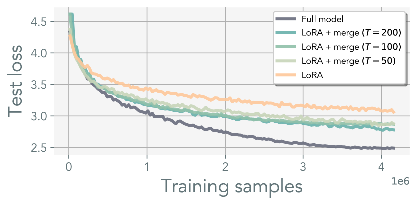
Figure 6: Sequential merging of LoRA cannot recover performance. ViT-S trained on ImageNet100. Merging and resetting the LoRA parameters achieves better performance than single-head LoRA pre-training but still cannot recover the standard full-model pre-training. Note that LoRA + merge is akin to concurrent work of ReLoRA (Lialin et al., 2023).

4.1 Iterative LoRA Merging

In Section 3.1, we motivated that iteratively merging LoRA parameters is a key component in accurately recovering the full-rank representation of the model. As a sanity check, in Appendix A.3, we assess the effectiveness of merging a single LoRA head in the context of linear networks trained on synthetic least-squares regression datasets. The underlying rank of the optimal solution, $\mathbf{W}^{*}$, is controlled, and datasets are generated as $\mathbf{Y}=\mathbf{X}(\mathbf{W}^{*})^{\mathsf{T}}$. Each $\mathbf{x}\in\mathbf{X}$ follows a normal distribution, $\mathbf{x}\sim\mathcal{N}(\mathbf{0},\mathbf{I})$. Figure 11 evaluates the model’s rank recovery across varying merge iteration $T$. Dimension of the weights $\mathbf{W}$ are set to $m=n=32$. Without merging, the model performance plateaus rapidly on full-rank $\mathbf{W}^{*}$. In contrast, iterative merging recovers the ground truth solution with the rate increasing with higher merge frequency.

Further tests in Figure 6 using ViT-S (Dosovitskiy et al., 2020) with a patch-size of 32 on the ImageNet100 dataset (Tian et al., 2020) (a subset of ImageNet (Russakovsky et al., 2015)) confirm that merging of a single LoRA head outperforms standalone LoRA parameter training. However, frequent merging delays convergence, likely due to LoRA parameter re-initialization and momentum state inconsistencies. Additionally, the performance does not match that of fully trained models, indicating potential local minima when training with rank-deficient representations.

We find that the merge iteration of $T=10$ is still stable when using batch size $4096$. With higher $T$ values, additional training may be required to achieve comparable performance (Stich, 2019; Wang & Joshi, 2021; Yu et al., 2019). Our initial efforts to improve merging using methods such as (Yadav et al., 2023) did yield better results. Nonetheless, we believe with increased merge iteration, smarter merging techniques may be necessary. Existing literature in federated learning and linear-mode connectivity/model-averaging may provide insights in designing better merging criteria.

To further test the generalizability of our method, we conducted a suite of experiments on various vision tasks in Figure 7. Moreover, we test our method on MLP-Mixer (Tolstikhin et al., 2021) to demonstrate its use outside of transformer architecture. We provide additional experiments when using $T=1$ and initial language-modeling results in Appendix D.

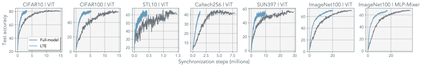
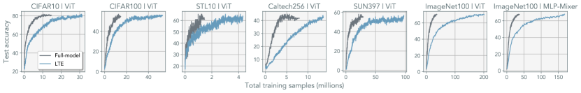
Figure 7: Experiments on various vision tasks: We apply our method to a range of vision tasks, including CIFAR10, CIFAR100 (Krizhevsky et al., 2009), STL10 (Coates et al., 2011), Caltech256 (Griffin et al., 2007), SUN397 (Xiao et al., 2010), and ImageNet100 (Tian et al., 2020). Details of these datasets are listed in Appendix 4. Additionally, we incorporated the MLP-mixer and observed consistent results. The figure is presented with two different x-axes. On the top, we plot the total number of synchronization steps, and on the bottom, we measure the total number of training samples observed across all devices. All LTE experiments are conducted on ViT-S with a merge iteration of $T=10$ and 32 LoRA heads with a rank of $r=64$. In Appendix D, we provide additional results for $T=1$, LLM experiments, and LTE trained on ViT and MLP-mixer at various scales.

4.2 LoRA parameter alignment

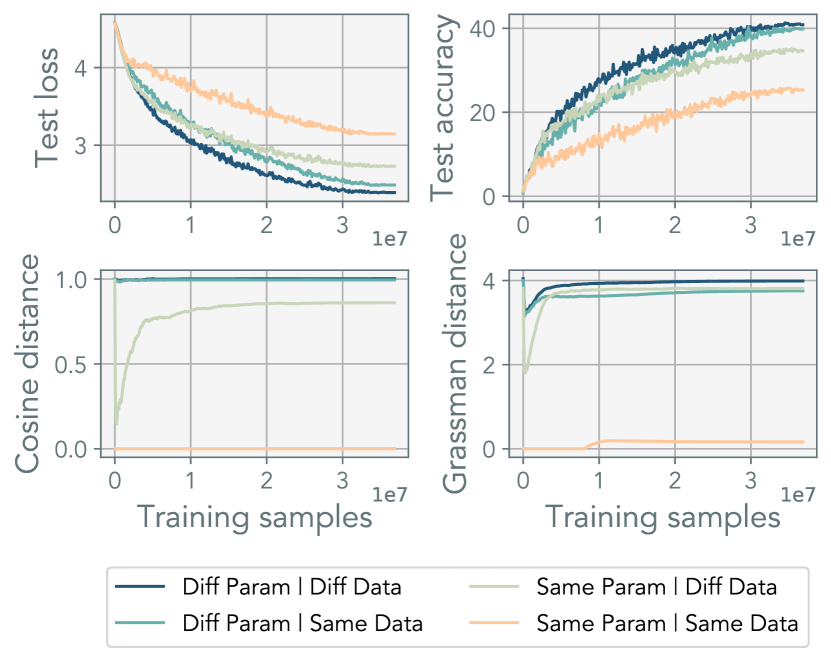
Figure 8: LoRA alignment: Alignment of LTE heads when varying parameters and data. “Diff Param” uses random initialization across each head, and “Diff Data” uses different mini-batches. The similarity is computed on the first epoch of ImageNet100 on ViT-S. We use LTE of $r$=$8$ with $4$ LoRA heads. Pair-wise similarity is averaged across all linear layers. The performance of the model correlates with orthogonality between LoRA heads.

The efficacy of our optimization algorithm hinges on the ability of individual heads to explore distinct subspaces within the parameter space. We examine the extent to which data and initial parameters influence intra-head similarity throughout training. In Figure 8, we compute the average cosine similarity and Grassman distance (see Appendix A.5) between the heads $\mathbf{B}_{n}\mathbf{A}_{n}$. These tests were conducted with data samples drawn from the same distribution, and each set of LoRA parameters was exposed to a different set of samples.

Our results confirm that LoRA heads do not converge to the same representation. We find using different initializations across LoRA heads yields the greatest orthogonality. This orthogonality is further increased when different mini-batches are used for each head. Importantly, the degree of alignment among LoRA heads remains stable post-initialization and does not collapse into the same representation. In Figure 8, we find that lower similarity corresponds well with model performance, where using different parameters and mini-batches significantly outperforms other configurations.

	LTE	Heads	Rank	Merge	Test loss $\downarrow$	Test acc $\uparrow$
	-	-	-	-	1.78	71.97
$\mathsf{head}$	✓	2	8	10	2.31	54.68
	✓	8	8	10	2.35	54.88
	✓	32	8	10	2.26	58.21
	✓	2	64	10	1.86	69.82
	✓	8	64	10	1.84	71.97
	✓	32	64	10	1.79	73.73
$\mathsf{rank}$	✓	32	8	10	2.66	44.00
	✓	32	16	10	2.12	60.35
	✓	32	32	10	1.81	71.20
	✓	32	64	10	1.79	73.73
	✓	32	128	10	1.78	73.54
$\mathsf{merge}$	✓	32	64	5	1.87	70.67
	✓	32	64	10	1.79	73.73
	✓	32	64	20	1.97	66.80
	✓	32	64	50	1.99	65.43
	✓	32	64	100	2.10	61.04

Table 1: LTE ablation for ViT-S trained ImageNet100: For fixed cumulative training epoch of $1200$, we vary the number of heads, rank, and merge iteration of our method. More heads require longer cumulative training samples to converge; see Figure 9.

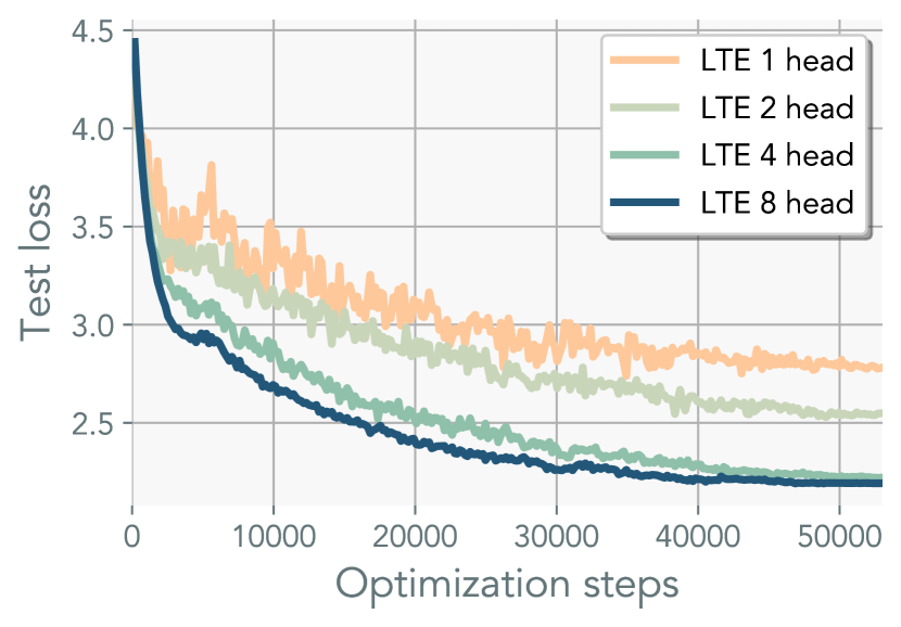
Figure 9: LTE with same batch-size per head: ViT-S trained on ImageNet100. We use the same batch-size for each LoRA head with rank $r=8$. In contrast to other figures, we plot the loss in optimization steps. LTE with more heads converge to a better solution but require longer training samples to converge.

4.3 Ablation study: the effect of LoRA heads, rank, and merge iteration

We systematically evaluate the effects of varying the number of LoRA heads, rank, and merge iteration on model performance for ImageNet100 in Table 1. Our findings indicate a monotonic improvement in performance with an increased number of heads and ranks. Conversely, extending the merge iteration negatively impacts performance. As in the case of least-squares regression, we found excessive merging to hurt model accuracy. With a large enough rank and head, we found the model to converge to better test accuracy, even if the test loss was similar. We hypothesize the averaging of the LoRA heads has a regularization effect similar to that model ensembling.

We use ViT-S as the primary architecture for analysis, which has a hidden dimension of $384$ and an MLP dimension of $1536$. We find that setting the product of the number of heads and the rank of the LoRA larger than the largest dimension of the model serves as a good proxy for configuring LTE. For example, using $32$ heads with $r=64$ results in $2048>1536$. However, when it comes to increasing the number of heads rather than rank, we noticed longer training iterations were required to achieve comparable performance. We discuss a potential cause of the slowdown in convergence in the preceding section.

4.4 Gradient noise with parallel updates

In our ablation study, we utilized a fixed cumulative batch size of $4096$ and a training epoch of $1200$. Each LoRA head received a reduced batch size of $\frac{4096}{\text{heads}}$. Our findings indicate that scaling the rank exerts a greater impact than increasing the number of heads. Due to the proportional scaling of gradient noise with smaller mini-batches (McCandlish et al., 2018; Shallue et al., 2019; Smith & Le, 2018), we hypothesize that gradient noise is the primary factor contributing to slower convergence, in addition to the use of stale parameter estimates. To validate this hypothesis, we employed the same mini-batch size across all heads in Figure 9, using a reduced rank of $r=8$. When we adjusted the batch size in proportion to the number of heads and measured it with respect to the optimization steps, the impact of varying the number of heads became more pronounced. While increasing the number of heads necessitates more sequential FLOPs, it offers efficient parallelization. Furthermore, using a larger batch size for gradient estimation may prove beneficial in distributed training, as it increases the computational workload on local devices. Careful optimization of the effective batch size to maximize the signal-to-noise ratio may be crucial for achieving maximum FLOP efficiency.

Figure 10: ImageNet compute analysis: We break down the computational cost for training ViT-S on ImageNet1k. We compare against distributed data-parallel with $8$ devices. LTE requires $40\%$ longer to achieve the same performance of $68\%$ top-1 accuracy on $1000$-way classification. We used $32$ LoRA heads with $r=64$. Our method requires fewer trainable parameters per device. This, in turn, enables the fitting of larger models in low-memory devices. With a smaller memory footprint and infrequent communication, our method requires lower communication bandwidth. Further discussion is in Section 4.5.

4.5 Performance Scaling on ImageNet-1K

We scaled up our method to ImageNet-1K. We followed the training protocols detailed in Appendix A.1. In accordance with our initial hypothesis on gradient noise, we doubled the batch size to $8192$ (see Appendix A.7). Since using different mini-batches was crucial early in training, we did not alter the way mini-batches were sampled. Scheduling the randomness for the mini-batches is an option we have not yet explored.

In the initial training phase, we observed that LTE outperformed standard training. However, as training approached completion, standard training overtook LTE, necessitating additional iterations for LTE to achieve comparable performance. Standard training appeared to benefit more from a lower learning rate compared to LTE. For ViT-S, the model took $40\%$ more training samples to converge to the same top-1 accuracy of $68\%$ (see Appendix A.6).

The primary focus of our work was to investigate whether it is possible to train deep networks with parallel low-rank adapters; hence, we did not aim to maximize efficiency. However, we do provide a hypothetical computation analysis for future scaling efforts. Let the model size be denoted by $M_{\mathsf{ddp}}=M$, and $M_{\mathsf{lte}}$ for LTE, and the respective number of devices for each method be denoted with $N_{\mathsf{ddp}}$, and $N_{\mathsf{lte}}$. With quantization, each LTE device would require a memory footprint of $qM+M_{\mathsf{lte}}$. With the base model operating in 16-bit precision, using 4-bit quantization results in $q=0.25$. With AdamW, DDP necessitates an additional $2M$ parameters, making the total memory footprint $3M$ per device. For LTE, the total memory footprint per device is $qM+3M_{\mathsf{lte}}$. Assuming the training is parameter-bound by the main weights $r\ll\min(m,n)$, LTE can leverage GPUs that are roughly $1/3$ the size required for DDP. It is worth noting that LTE requires $40\%$ more data to train and a slowdown of $20\%$ per iteration when using quantization methods such as QLoRA. If the cost of low-memory devices is lower, these slowdowns may be negligible compared to the speed-up achieved through parallelization. On average, each LTE device observes $1/3$ less data than a device in DDP. With improvements in our method and future advances in quantization, we believe this gap will be reduced. The compute analysis for ViT-S on ImageNet1k is illustrated in Figure 10.

Communication also presents bottlenecks when training models across nodes. For a single node, one can interleave the communication of gradients asynchronously with the backward pass (Li et al., 2020a). In multi-node systems, the communication scales with the size of the trained parameters and is bottlenecked at interconnect speed, especially when high-throughput communication hardware, such as InfiniBand, is not utilized. Using standard all-reduce, the gradient is shared between each device for a total communication of $N_{\mathsf{ddp}}(N_{\mathsf{ddp}}-1)M$. For LTE we communicate every $T$ iteration hence we have $\frac{1}{T}N_{\mathsf{lte}}(N_{\mathsf{lte}}-1)M$. To maximize the efficacy of LTE, an alternative approach is to use a parameter server for 1-and-broadcast communication. Here, gradients are sent to the main parameter server and averaged. The accumulated updates are broadcast back to other nodes. DDP with a parameter server would use $2(N_{\mathsf{ddp}}-1)M$ and LTE would use $\frac{1}{T}((N_{\mathsf{lte}}-1)M_{\mathsf{lte}}+(N_{\mathsf{lte}}-1)qM)$. Moreover, LTE can leverage lower-bandwidth communication since the parameters shared between devices are strictly smaller by a factor of $M_{\mathsf{ddp}}/M_{\mathsf{lte}}$.

5 Related works

Training with adapters

The use of LoRA has garnered considerable attention in recent research. While our work focuses on using adapters to pre-train model from scratch, majority of the works have focused on enhancing finetuning processes through these adapters (Chavan et al., 2023; Zhang et al., 2023b), while others aim to diminish computational requirements (Zhang et al., 2023a) or to offset part of the pre-training computation (Lialin et al., 2023). Moreover, motivated by (Wortsman et al., 2022), (Wang et al., 2022) proposes the use mixture-of-expert for parameter efficient finetuning and uses averaging for efficient inference. Various forms of adapters have been proposed in prior research, each serving specific applications. Additive adapters (Zhang et al., 2021) augment the model size for inference, and hence the community has turned towards linear adapters either in the form residual connections (Cai et al., 2020) or affine parameters in batch-norm, (Bettelli et al., 2006; Mudrakarta et al., 2018). Adapters have been applied for natural language processing (Houlsby et al., 2019; Stickland & Murray, 2019), video (Yang et al., 2024b; Xing et al., 2023), computer vision (Sax et al., 2020; Zhang & Agrawala, 2023; Chen et al., 2023), incremental learning (Rosenfeld & Tsotsos, 2018), domain adaptation (Rebuffi et al., 2018), and vision-language tasks (Gao et al., 2023; Radford et al., 2021; Sung et al., 2022), text-to-vision generative models (Mou et al., 2023), and even perceptual learning (Fu et al., 2023).

Distributed Training and Federated Learning

Our work has relevance to both distributed and federated learning paradigms, wherein each head is conceptualized as a distinct computational device. Federated learning addresses various topics, including low-compute devices, high-latency training, privacy, and both cross and in-silo learning, as comprehensively discussed in (McMahan et al., 2017; Wang et al., 2021). Communication efficiency serves as a cornerstone in both distributed and federated learning. Techniques such as local steps have been employed to mitigate communication load (McMahan et al., 2017; Lin et al., 2020; Povey et al., 2014; Smith et al., 2018; Su & Chen, 2015; Zhang et al., 2016). These methods defer the averaging of weights to specific optimization steps, thus alleviating the communication cost per iteration. The effectiveness of decentralized training has been studied in (Lian et al., 2017; Koloskova et al., 2019, 2020; Coquelin et al., 2022). Traditionally, activation computations have dominated the computational load. However, the advent of gradient checkpointing (Chen et al., 2016) and reversible gradient computation (Gomez et al., 2017; Mangalam et al., 2022) has shifted the training process toward being increasingly parameter-bound. Techniques such as gradient or weight compression also seek to reduce the communication burden (Lin et al., 2018; Aji & Heafield, 2017; Wen et al., 2017). Combining models in federated learning is often credited to FedAvg (McMahan et al., 2017). Numerous studies explore the use of weighted averaging to improve convergence speed (Li et al., 2020b). Since then, many works have tried to use probabilistic frameworks to understand and improve merging (Hsu et al., 2019; Wang et al., 2020; Reddi et al., 2021). The conditions for optimal merging is still an open question, with recent efforts to improve updating with stale parameters has been explored in (Chen et al., 2022). Server momentum and adaptive methods constitute another active area of research where macro synchronization steps may be interpreted as gradients, thus facilitating bi-level optimization schemes (Hsu et al., 2019; Wang et al., 2020; Reddi et al., 2021). Initial efforts to employ federated learning with large models have been made. (Yuan et al., 2022) examined the cost models for pre-training Language Learning Models (LLMs) in a decentralized configuration. (Wang et al., 2023) suggested the utilization of compressed sparse optimization methods for efficient communication.

Linear mode connectivity and model averaging

Linear mode connectivity (Garipov et al., 2018) pertains to the study of model connectivity. Deep models are generally linearly disconnected but can be connected through nonlinear means (Freeman & Bruna, 2017; Draxler et al., 2018; Fort & Jastrzebski, 2019). Under the same initialization, linear paths with constant energy exist in trained models (Nagarajan & Kolter, 2019; Frankle et al., 2020; Wortsman et al., 2022). For models with different initializations, parameter permutations can be solved to align them linearly (Brea et al., 2019; Tatro et al., 2020; Entezari et al., 2021; Simsek et al., 2021). Following this line of research, numerous works have delved into model averaging and stitching. Where averaging of large models has shown to improve performance (Wortsman et al., 2022; Ainsworth et al., 2023; Stoica et al., 2024; Jordan et al., 2023). Model stitching (Lenc & Vedaldi, 2015) has also shown to yield surprising transfer capabilities (Moschella et al., 2023). This idea is conceptually related to optimal averaging in convex problems (Scaman et al., 2019) and the “Anna Karenina” principle where successful models converge to similar solutions (Bansal et al., 2021). The effectiveness of averaging models within ensembles is well-established (Huang et al., 2017; Izmailov et al., 2018; Polyak & Juditsky, 1992). Utilizing an average model as a target has also been investigated (Tarvainen & Valpola, 2017; Cai et al., 2021; Grill et al., 2020; Jolicoeur-Martineau et al., 2023; Wortsman et al., 2023).

6 Conclusion

In this work, we investigated the feasibility of using low-rank adapters for model pre-training. We introduced LTE, a bi-level optimization method that capitalizes on the memory-efficient properties of LoRA. Although we succeeded in matching performance on moderately sized tasks, several questions remain unresolved. These include: how to accelerate convergence during the final $10\%$ of training; how to dynamically determine the number of ranks or heads required; whether heterogeneous parameterization of LoRA is feasible, where each LoRA head employs a variable rank $r$; and leveraging merging strategies to accompany higher local optimization steps. Our work serves as a proof-of-concept, demonstrating the viability of utilizing low-rank adapters for neural network training from scratch. However, stress tests on larger models are essential for a comprehensive understanding of the method’s scalability. Addressing these open questions will be crucial for understanding the limitations of our approach. We anticipate that our work will pave the way for pre-training models in computationally constrained or low-bandwidth environments, where less capable and low-memory devices can collaboratively train a large model, embodying the concept of the “wisdom of the crowd.”

7 Acknowledgement

JH is supported by the ONR MURI grant N00014-22-1-2740 and the MIT-IBM Watson AI Lab. JB is supported by the MIT-IBM Watson AI Lab and the Packard Fellowship. PI is supported by the Packard Fellowship. BC is supported by the NSF STC award CCF-1231216. We thank Han Guo, Lucy Chai, Wei-Chiu Ma, Eunice Lee, and Yen-Chen Lin for their feedback.

Appendix A Appendix

A.1 Training details

Training details:   We adhere to the standard training protocols. Below are the references:

Vision training code	PyTorch TorchVision references
ViT implementation	PyTorch TorchVision models
MLP-mixer implementations	huggingface/pytorch-image-models
Quantization	TimDettmers/bitsandbytes

We replace the fused linear layers with standard linear layers to use LoRA. LoRA is applied across all linear layers. All experiments incorporate mixed-precision training. For nodes equipped with 4 GPU devices, we implement gradient checkpointing. We used gradient checkpointing for ViT-B and ViT-L.

Hardware:   Our experiments were conducted using various NVIDIA GPUs, including V100 and Titan RTX.

Architecture detail:

Architecture	ViT-S	ViT-B	ViT-L
Patch-sizse	32	32	32
Attention blocks	12	12	24
Attention heads	6	12	16
Hidden dim	6	768	1024
MLP dim	1536	3072	4096
Total parameters	22.9M	88.2M	306.5M

Table 2: ViT architecture details.

Architecture	Mixer-T	Mixer-S	Mixer-B
Patch-sizs	32	32	32
Mixer blocks	6	8	12
Embed dim	384	512	768
MLP dim	1536	2048	3072
Total parameters	8.8M	19.1M	60.3M

Table 3: MLP-mixer architecture details

Architecture	NanoGPT	GPT2
Block-size	256	1024
Attention blocks	6	12
Attention heads	6	12
Hidden dim	384	768
MLP dim	1152	2304
Total parameters	10.7M	124.4M

Table 4: LLM GPT architecture details.

Dataset details:

Dataset	CIFAR10	CIFAR100	STL10	CALTECH256	SUN397	ImageNet100	ImageNet1K
Original image-size	$32\times 32$	$32\times 32$	$96\times 96$	Variable	Variable	Variable	Variable
Training image-size	$224\times 224$	$224\times 224$	$224\times 224$	$224\times 224$	$224\times 224$	$224\times 224$	$224\times 224$
Number of classes	$10$	$100$	$10$	$257$	$397$	$100$	$1,000$
Number of images	$60,000$	$60,000$	$13,000$	$30,607$	$108,754$	$130K$	$>$1.2M
Learning-rate $\eta_{\mathsf{default}}$	$3\cdot 10^{-4}$	$3\cdot 10^{-4}$	$3\cdot 10^{-4}$	$3\cdot 10^{-4}$	$3\cdot 10^{-3}$	$3\cdot 10^{-3}$	$3\cdot 10^{-3}$
Learning-rate $\eta_{\mathsf{lte}}$	$2\cdot 10^{-5}$	$2\cdot 10^{-5}$	$2\cdot 10^{-5}$	$2\cdot 10^{-5}$	$5\cdot 10^{-6}$	$3\cdot 10^{-5}$	$3\cdot 10^{-5}$
Batch-size	$1024$	$1024$	$1024$	$1024$	$1024$	$4096$	$8192$

Table 5: Specifications for vision datasets. Most dataset images indicated as “variable size” are larger than the training image size. We provide training configuration used for ViT. For MLP-Mixer on ImageNet100, we use a learning rate of $0.001$ for full-model pre-training and $1\cdot 10^{-4}$ for LTE, both with a batch size of 4096.

Dataset	Shakespeare	TinyStories
Total number of tokens	$1.0M$	$474.0M$
Tokenizer size	$65$	$50304$
Learning-rate $\eta_{\mathsf{default}}$	$1\cdot 10^{-3}$	$6\cdot 10^{-4}$
Learning-rate $\eta_{\mathsf{lte}}$	$2\cdot 10^{-6}$	$5\cdot 10^{-5}$
Batch-size	$512$	$512$
Block-size	$256$	$1024$

Table 6: Specifications for LLM datasets and hyper-parameters used for miniGPT on Shakespeare and GPT2 on Tinystories.

LTE Optimization Details:   We use $\alpha=4096\sim 8192$, which is $s=128\sim 256$ when $r=32$ and $s=64\sim 128$ when $r=64$. A good rule of thumb for the learning rate is to set it at approximately $0.1\sim 0.05\times$ the standard model training learning rate. We use the same learning rate scheduler as the standard pre-training, which is cosine learning-rate decay with linear warmup.

LTE Batching Detail:   We use a fixed cumulative batch size for LTE. This means that given a batch size $B$ with $N$ LoRA heads, each head receives a batch size of $[B/N]$. When counting the training iterations, we count $B$ and not $[B/N]$. Counting using $[B/N]$ would significantly inflate our numbers, but in the federated learning community, it is referred to as “synchronization steps”. LTE training epochs were set to $4\times$ the cumulative batch size, and we exited early when we matched the performance of full-model training. For smaller datasets, our method seemed to consistently outperform the baseline, likely due to the regularization properties of rank and over-parameterization.

LTE Implementation Details:   We implemented LTE using Parameter Server, model-parallelism, and DDP. Parameter server is theoretically more beneficial for our method, we conducted most of our development using DMP and DDP as it does not require rewriting communication logic. We utilize ‘torch.vmap’ and simulate multiple devices on the same GPU, and share computation of the main parameters to reduce run-time.

LTE for Convolution, Affine, and Embedding Layers:   Specific choices for all these layers did not impact the final performance significantly, but we detail the choices we made below.

For convolution layers, we use the over-parameterization trick in (Huh et al., 2023), which uses $1\times 1$ for the second layer. Since convolution layers are typically used at most once in the models we tested, we did not explore beyond this parameterization. However, other potential choices exist for low-rank parameterization of convolution layers, such as channel-wise convolution and separable convolutions.

There is no notion of low-rank decomposition for affine parameters used in normalization layers. We tried various strategies to train and communicate these parameters. For affine parameters, we tried: (1) LoRA-style vector-vector parameterization $\textbf{a},\textbf{b}$, (2) LoRA-style vector-scalar parameterization $\textbf{A}=\textbf{a},b$, (3) DDP-style averaging, and (4) removing affine parameters. Removing affine parameters improved both baseline and LTE for classification.

Lastly, we found that using the standard averaging technique or allowing only one model to train the embedding layer worked best for the embedding layer. We chose to use standard averaging at the same iteration as the rest of the LoRA layers.

A.2 Getting exact equivalence

The exact equivalence condition for LTE and MHLoRA is achieved when the LoRA parameters are not reset. Empirically, this does lead to slightly better model performance but requires a more involved calculation. We posit that the slight improvement comes from the fact that we do not have to re-learn the LoRA parameters and ensure the optimizer state is consistent with respect to its parameters. We provide the exact equivalence below.

Denote $t$ as the synchronization steps, $\tau$ as the local optimization step:

$$\underset{\mathbf{B}_{0},\mathbf{A}_{0},\dots\mathbf{B}_{N},\mathbf{A}_{N}}{\text{optimize}}\quad\mathbf{W}\mathbf{x}+\frac{s}{N}\sum_{i=1}^{N}\mathbf{B}_{i}^{(t,\tau)}\mathbf{A}_{i}^{(t,\tau)}\mathbf{x}$$

To match the gradient dynamics exactly, one needs to merge all LoRA and subtract the contribution of its weight after the merge. Denote $\mathbf{V}$ as the previous LoRA parameter contribution and is set to $\mathbf{0}$. Then, the LTE optimization with the correction term is:

Where the equivalence to multi-head LoRA holds when $\tau=1$. Note that the subtracting of the previous contribution can be absorbed into the weight $(\mathbf{W}^{(t)}-s\mathbf{V}_{i}^{(t)})\mathbf{x}$.

A.3 Merge with least-squares

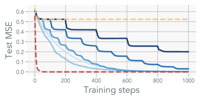
Figure 11: Least-squares with LoRA: Linear models parameterized with LoRA with varying target rank. Least-squares with $\mathbb{R}^{32\times 32}$, with target rank of $32$ (right) and $8$ (left). LoRA is parameterized with rank $r=4$. With merging, the model can recover the solution, with convergence scaling with merge frequencies.

We train a linear network, parameterized with LoRA, on least-squares regression. Here, we artificially constructed the problem to control for the underlying rank of the solution $\mathbf{W}^{*}$. We then constructed a dataset by randomly generating $\mathbf{Y}=\mathbf{X}(\mathbf{W}^{*})^{\mathsf{T}}$. Where for each element $\mathbf{x}\in\mathbf{X}$ is drawn from a normal distribution $\mathbf{x}\sim\mathcal{N}(\mathbf{0},\mathbf{I})$.

Figure 11 visualizes the model’s ability to recover the underlying ground-truth solution across various merge iterations $T$. Here, the optimal solution $\mathbf{W}^{*}$ is set to be full rank where $m=n=32$. We employ a naive re-initialization strategy of initializing $\mathbf{A}$ with a uniform distribution scaled by the fan-out.

Without merging the LoRA parameters, the model’s performance rapidly plateaus. In contrast, models trained with merges can eventually recover the full-rank solution, with the recovery rate of the solution scaling with the merging frequency.

A.4 Ablation

We conducted an ablation study focusing on initialization, resetting of LoRA $\mathbf{A}$, and resetting the optimizer for the LoRA parameters. All ablation studies presented here were conducted with an LTE with rank $r=16$, $8$ heads using ViT-S on ImageNet100.

Kaiming initialization serves as the default scheme for LoRA. The conventional Kaiming initialization is tailored for square matrices and depends solely on the input dimension. Given that LoRA parameters often manifest as wide matrices, we experimented with various initialization schemes. Xavier initialization ((Glorot & Bengio, 2010)) preserves the variance relationship of a linear layer for rectangular matrices. Bernstein et al. ((Bernstein et al., 2023)) employ semi-orthogonal initialization to maintain the spectral norm of the input. As depicted in Figure LABEL:subfig:init_ablation_losses, the method by Bernstein et al. proved most effective. It should be noted that none of these initialization methods assume residual connection or zero-ed out LoRA parameters. Hence, further tuning of the gain parameters might be needed.

When resetting the LoRA parameters, we investigated the impact of re-initializing the matrix $\mathbf{A}$ as well as its optimizer. As shown in Figure LABEL:subfig:A_reset_ablation, we found that resetting matrix $\mathbf{A}$ adversely affects model performance, possibly due to the necessity of re-learning the representation at each iteration and discarding the momentum states. In Figure LABEL:subfig:opt_reset_ablation, we also experimented with retaining the LoRA parameters while resetting the optimizer state for those parameters. Similarly, we found that resetting the optimizer state diminishes performance.

A.5 Grassman distance of LoRA heads

Motivated by (Hu et al., 2022), we measure the Grassman distance of the LoRA heads to measure sub-space similarity between the optimized sub-spaces. Grassman distance measures the distance of $k$-dimensional subspace in a $n$-dimensional space. The distance is defined as:

For LoRA, the number of principal components is spanned by the LoRA rank $r$; therefore, we set $k=r$. When the LoRA parameters span the same sub-space, they have a Grassman distance of $0$. The pairwise Grassman distance is measured by:

$$\frac{1}{2N}\sum_{(i,j)\in[1,N]\land i\neq j}d_{\mathsf{Grassman}}(f_{\perp}(\mathbf{B}_{i}\mathbf{A}_{i}),f_{\perp}(\mathbf{B}_{j}\mathbf{A}_{j}),r)$$ (4)

Where $f_{\perp}(\cdot)$ computes the orthogonal basis by computing the input matrix’s left singular vectors.

A.6 Training curve on ImageNet1k

Figure 14: ImageNet1k test curve

We plot the test curves in Figure 14 for both standard and LTE training on ImageNet-1K. Both models were trained using a cosine learning rate scheduler. We found that training LTE for $300$ epochs performed roughly $5\%$ worse. Hence, we repeated the experiment by setting the training epoch to $600$. The final performance was matched at around $420$ epochs. For LTE, we doubled the batch size to $8192$ (see Appendix A.7). We found that LTE benefits from larger cumulative batch size and does not require as intensive of data augmentation as standard training, likely due to implicit regularization induced by low-rank parameterization and stale updates. The baseline did not improve when using a bigger batch size. In simpler tasks, using bigger-batches did not perform better.

Early in the training phase, the baseline outperformed LTE, but this trend was quickly reversed after the first initial epochs. LTE approached its final performance quite rapidly. However, LTE fell short compared to the standard training duration by 300 epochs, and an additional $120$ epochs were required to reach the same test accuracy. Unlike LTE, we found that standard training benefited significantly more from the learning-rate scheduler, possibly hinting that the gradient noise and stale parameter estimates overpower the signal-to-noise ratio. We observed this trend across all ViT sizes.

A few ways to mitigate the slow convergence include synchronizing the mini-batches or the LoRA parameters as the model is trained; we leave such investigation for future works. The baseline was trained with a weight-decay of $0.01$, resulting in slow convergence but better final performance – standard optimization does exhibit faster convergence if the weight-decay is removed. Training the baseline for longer, $600$ epochs, did not achieve better performance.

A.7 Effect of batch-size on ImageNet1k

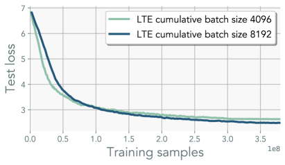
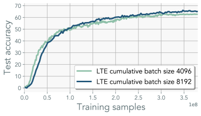
Figure 15: ImageNet1k with doubled accumulative batch-size

Utilizing larger batch sizes is beneficial for maximizing FLOP efficiency. However, when evaluated in terms of samples seen, larger batch sizes are known to underperform (Masters & Luschi, 2018). Given that LTE introduces more noise, we hypothesized that a reduced learning rate could be adversely affected by both gradient noise and estimate noise from using merges. In Figure 15, we experimented with increasing the batch size and observed a moderate improvement of $3\%$ with bigger batches.

Appendix B Rank of the model in pre-training

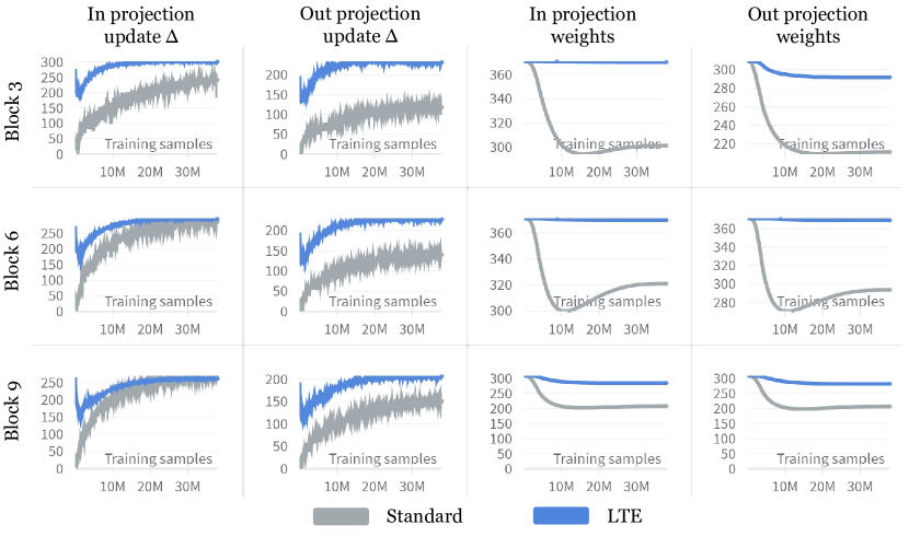
Figure 16: Rank dynamics of ViT for standard training and LTE. Rank is measured using effective rank. We track the rank of the weights and update to the main weight throughout training.

We measure the effective rank (Roy & Vetterli, 2007) of standard training and LTE throughout training.

The rank of the updates for standard training is the gradients, and LTE is $\nabla_{\mathbf{W}}\mathcal{L}$ and $\frac{s}{N}\sum_{n}\mathbf{B}_{n}\mathbf{A}_{n}$ respectively. In the context of standard training, the rank of the weights exhibits only a minor decrease throughout the optimization process. Conversely, the rank of the gradient monotonically increases following the initial epochs. This observation provides empirical evidence that approximating the updates with a single LoRA head is not feasible. Despite its markedly different dynamics, LTE can represent full-rank updates throughout the training period. This may also be useful for designing how many LoRA heads to use with LTE, where the number of LoRA heads can start with one and slowly annealed to match the maximum rank of the weights.

B.1 Is scaling $s$ the same as scaling the learning rate?

There is a misconception that the scalar $s$ only acts as a way to tune the learning rate in these updates. Focusing on the update for $\mathbf{B}$ (same analysis holds for $\mathbf{A}$), we can write out the gradient as:

$$g(\mathbf{B})=\frac{\partial\mathcal{L}}{\partial\mathbf{B}}=s\frac{\partial\mathcal{L}}{\partial\mathbf{z}_{out}}(\mathbf{A}\mathbf{z}_{in})^{T}=s\bar{g}_{t}$$ (5)

If we were using stochastic gradient descent, we would expect $s$ to behave like a linear scaling on the learning rate:

$$\Delta(\mathbf{B})=-\eta s\bar{g}$$ (6)

Where we denoted $\bar{g}$ as the component of the gradient with $s$ factored out. We now show that $s$ does not linearly scale the learning rate for Adam (this analysis can be extended to scale-invariant optimizers). Adam is a function of the first-order momentum $m_{t}$ and second-order momentum $v_{t}$. One can factor out $s$ from the momentum term: $m_{t}=s\hat{m}_{t}=s\beta_{1}\hat{m}_{t-1}+(1-\beta_{1})\hat{g}_{t}$ and $v_{t}=s^{2}\hat{v}_{t}=s^{2}\beta_{1}\hat{v}_{t-1}+(1-\beta_{1})\hat{g}_{t}^{2}$. Incorporating the gradient into the update rule, we see that the adaptive update does not depend linearly on $s$:

$$\Delta(\mathbf{B})=-\eta\frac{m_{t}}{\sqrt{v_{t}+\epsilon}}=-\eta\frac{{\color[rgb]{1,0,0}s}\hat{m}_{t}}{\sqrt{{\color[rgb]{1,0,0}s^{2}}\hat{v}_{t}+\epsilon}}=-\eta\frac{\hat{m}_{t}}{\sqrt{\hat{v}_{t}+\epsilon}}$$ (7)

However, $\hat{g}_{t}$ is not invariant to $s$. Therefore, while $s$ is not the same as the learning rate, it will impact the downward gradient $\frac{\partial\mathcal{L}(\dots,{\color[rgb]{1,0,0}s})}{\partial\mathbf{z}_{out}}$. We will discuss this in the next subsection. It is worth noting that $s$ quadratically impacts the attention map and may require a separate scaling factor as opposed between MLP layers and attention layers. Consider a batched input $\mathbf{X}$ with the output of a linear as $\hat{\mathbf{X}}=\mathbf{W}\mathbf{X}+{\color[rgb]{1,0,0}s}\mathbf{B}\mathbf{A}\mathbf{X}=\mathbf{W}\mathbf{X}+s\mathbf{D}$. Then, the un-normalized attention map is dominated by the LoRA parameters:

$$\left(\mathbf{W}_{Q}\hat{X}\right)\left(\mathbf{W}_{K}\hat{X}\right)^{T} =\mathbf{W}_{Q}\left(\mathbf{W}\mathbf{X}+s\mathbf{D}\right)\left(\mathbf{X}^{T}\mathbf{W}^{T}+s\mathbf{D}^{T}\right)\mathbf{W}_{K}^{T}$$ (8)

$$=\dots+{\color[rgb]{1,0,0}s^{2}}\mathbf{W}_{Q}\mathbf{D}\mathbf{D}^{T}\mathbf{W}_{K}^{T}$$ (9)

Unlike learning rate, scaling $s$ affects both the forward and backward dynamics. Large $s$ emphasizes the contribution of the LoRA parameters, which may explain why we have observed better performance when using larger $s$ for pre-training. It is possible that using a scheduler for $s$ could further speed up training or even better understand how to fuse $s$ into the optimizer or $\mathbf{A}$; we leave this for future work. Next, we dive into the effect of $s$ on $\bar{g}_{t}$.

B.2 The effective update rule for LoRA is different from standard update

When $s$ is small, we can safely discard the second term as it will scale quadratically with learning rate $\eta\hat{g}$. However, when $s$ is large, the contribution of the second term becomes non-negligible. This term can be interpreted as the alignment of the LoRA parameters, and taking a step in this direction encourages $\mathbf{B}$ and $\mathbf{A}$ to be spectrally aligned. The increased contribution of the LoRA parameters and the alignment induced by larger $s$ may explain our observation that higher $s$ leads to better performance. It’s important to note that with a learning rate scheduler, the contribution of the second term would decay to zero.

B.3 Derivation

Over-parameterization or linear re-parameterization, in general, has a non-trivial effect on the optimization dynamics. Here, we analyze the update of the effective weight to point out a rather surprising interaction between $s$ and $\eta$. Consider a standard update rule for SGD for $\mathbf{z}_{in}\in\mathbb{R}^{n\times 1}$, and $\mathbf{z}_{out}\in\mathbb{R}^{m\times 1}$ and $\mathbf{W}\in\mathbb{R}^{m\times n}$:

$$g(\mathbf{W}) =\frac{\partial\mathcal{L}}{\partial\mathbf{W}}=\frac{\partial\mathcal{L}}{\partial\mathbf{z}_{out}}\frac{\partial\mathbf{z}_{out}}{\partial\mathbf{W}}=\frac{\partial\mathcal{L}}{\partial\mathbf{z}_{out}}\mathbf{z}_{in}^{T}$$ (11)

We will denote $g(\mathbf{W})=g$ from now on for clarity. For standard LoRA with parameters $\hat{\mathbf{W}}=\mathbf{W}+s\mathbf{B}\mathbf{A}$, where $\mathbf{B}\in\mathbb{R}^{m\times r}$, $\mathbf{A}\in\mathbb{R}^{r\times n}$, the update rule on the effective weight is:

$$\hat{\mathbf{W}} \leftarrow\mathbf{W}+s\left(\mathbf{B}-\eta\frac{\partial\mathcal{L}}{\partial\mathbf{B}}\right)\left(\mathbf{A}-\eta\frac{\partial\mathcal{L}}{\partial\mathbf{A}}\right)$$ (12)

$$=\mathbf{W}+s\mathbf{B}\mathbf{A}-s\eta\left(\left(\mathbf{B}\frac{\partial\mathcal{L}}{\partial\mathbf{A}}-\mathbf{A}\frac{\partial\mathcal{L}}{\partial\mathbf{B}}\right)+\eta\frac{\partial\mathcal{L}}{\partial\mathbf{B}}\frac{\partial\mathcal{L}}{\partial\mathbf{A}}\right)$$ (13)

We denote $g(\hat{\mathbf{W}})$ as $\hat{g}$. With the resulting effective update being:

$$\hat{g}=\left(\mathbf{B}\frac{\partial\mathcal{L}}{\partial\mathbf{A}}-\frac{\partial\mathcal{L}}{\partial\mathbf{B}}\mathbf{A}\right)-\eta\frac{\partial\mathcal{L}}{\partial\mathbf{B}}\frac{\partial\mathcal{L}}{\partial\mathbf{A}}$$ (14)

Computing the derivative for each variable introduces the dependency on $s$.

$$\frac{\partial\mathcal{L}}{\partial\mathbf{B}} =\frac{\partial\mathcal{L}}{\partial\mathbf{z}_{out}}\frac{\partial\mathbf{z}_{out}}{\partial\mathbf{z}_{res}}\frac{\partial\mathbf{z}_{res}}{\partial\mathbf{B}}=s\frac{\partial\mathcal{L}}{\partial\mathbf{z}_{out}}(\mathbf{A}\mathbf{z}_{in})^{T}$$ (15)

$$\frac{\partial\mathcal{L}}{\partial\mathbf{A}} =\frac{\partial\mathcal{L}}{\partial\mathbf{z}_{out}}\frac{\partial\mathbf{z}_{out}}{\partial\mathbf{z}_{res}}\frac{\partial\mathbf{z}_{res}}{\partial\mathbf{A}}=s\mathbf{B}^{T}\frac{\partial\mathcal{L}}{\partial\mathbf{z}_{out}}\mathbf{z}_{in}^{T}$$ (16)

Plugging it back in, we have

$$\hat{g} =\left(\mathbf{B}\left(s\mathbf{B}^{T}\frac{\partial\mathcal{L}}{\partial\mathbf{z}_{out}}\mathbf{z}_{in}^{T}\right)-\left(s\frac{\partial\mathcal{L}}{\partial\mathbf{z}_{out}}(\mathbf{A}\mathbf{z}_{in})^{T}\right)\right)\mathbf{A}-\eta\left(s\frac{\partial\mathcal{L}}{\partial\mathbf{z}_{out}}(\mathbf{A}\mathbf{z}_{in})^{T}\right)\left(s\mathbf{B}^{T}\frac{\partial\mathcal{L}}{\partial\mathbf{z}_{out}}\mathbf{z}_{in}^{T}\right)$$ (17)

$$=s\left(\frac{\partial\mathcal{L}}{\partial\mathbf{z}_{out}}\mathbf{z}_{in}^{T}\mathbf{A}^{T}\mathbf{A}-\mathbf{B}\mathbf{B}^{T}\frac{\partial\mathcal{L}}{\partial\mathbf{z}_{out}}\mathbf{z}_{in}^{T}\right)-s^{2}\eta\left(\frac{\partial\mathcal{L}}{\partial\mathbf{z}_{out}}\mathbf{z}_{in}^{T}\mathbf{A}^{T}\mathbf{B}^{T}\frac{\partial\mathcal{L}}{\partial\mathbf{z}_{out}}\mathbf{z}_{in}^{T}\right)$$ (18)

$$=s\left(\mathbf{B}\mathbf{B}^{T}g-g\mathbf{A}^{T}\mathbf{A}\right)-s^{2}\eta\left(g\mathbf{A}^{T}\mathbf{B}^{T}g\right)$$ (19)

When $s$ is small, both terms exist. When $s$ is large, the second term dominates. Since the last term is quadratic with $g$, one can safely ignore the second term when the learning rate is sufficiently small. Similarly, when using a learning rate scheduler, the contribution of the second term would decay to zero. The second term can be interpreted as an alignment loss where the gradient moves in the direction that aligns LoRA parameters.

Appendix C Method illustrations

In our illustrations, we detail the distinctions between our method and other common strategies. Distributed Data-Parallel (DDP) synchronizes the model at every iteration, with only the gradients being communicated between devices. This necessitates model synchronization across devices every iteration. Therefore, if there’s a significant delay in synchronization due to slow interconnect speeds or large model sizes, synchronization becomes a bottleneck. One way to mitigate this is through local optimization, often referred to as local steps or local SGD in federated learning. Here, instead of communicating gradients, model weights are shared. Local steps are known to converge on expectation, but they still require communicating the full model, which is loaded in half or full precision, which will quickly become infeasible in $1$B+ size models.

Our proposed method addresses both communication and memory issues by utilizing LoRA. Each device loads a unique set of LoRA parameters, and these parameters are updated locally. As discussed in our work, this enabled efficient exploration of full-rank updates. We communicate only the LoRA parameters, which can be set to be the order of magnitude smaller than the original model’s size. Our approach balances single-contiguous memory use with the ability to utilize more devices. The aim is to enable the training of large models using low-memory devices.

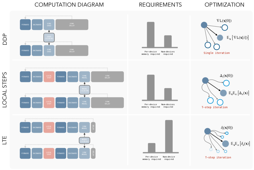
Figure 17: Method illustration: Comparisons between distributed learning methods to our method.

Appendix D Additional results

In all of our experiments, we present two distinct curves for analysis: one that represents the total training data observed across all devices and another that shows the training samples or tokens seen per device. We use LTE with $T=1$ for all experiments below, which is equivalent to the Multihead-LoRA optimization.

D.1 Vision Image Classification

We conduct additional experiments in image classification, covering datasets like CIFAR10 (Krizhevsky et al., 2009), CIFAR100 (Krizhevsky et al., 2009), STL10 (Coates et al., 2011), Caltech256 (Griffin et al., 2007), and SUN397 (Xiao et al., 2016). For these tests, we re-tuned all baseline learning rates. Detailed information about these datasets is available in Appendix A.1. For LTE, we use ranks of $r=64$ and $N=32$ heads.

D.2 Scaling up ViT model size

We train larger variants of the Vision Transformer (ViT) model. Details on these architectures are provided in Appendix A.1. Across all sizes, our results remained consistent, and for ViT-L, we used a rank of $r=128$.

D.3 LTE on MLP-Mixer

To evaluate the generalizability of our method to non-Transformer-based architectures, we train MLP-Mixer (Tolstikhin et al., 2021) using LTE. The specific details of the architecture used in datasets are listed in Appendix A.1. Our findings are consistent results across different scales of the MLP-Mixer. For Mixer-B, we use a rank of $r=128$.

D.4 Language Modeling

We also apply our method to language modeling. For these experiments, we utilized the nanoGPT codebase (Karpathy, 2023). Detailed information about the architectures and datasets employed can be found in Appendix A.1. Shakespeare’s dataset was trained using MiniGPT (Karpathy, 2023), while TinyStories (Eldan & Li, 2023) was trained on GPT2 (Radford et al., 2019). For Shakespeare, we used a configuration with rank $r=16$ and $N=32$ heads, and for TinyStories, we employed rank $r=64$ and $N=32$ heads. Consistent results were observed across all sizes. We observed on simple and small datasets that LTE has a beneficial regularization effect, reducing overfitting. Note: We did not increase the training duration for these experiments and used fixed cumulative training samples.

References

- Ainsworth et al. (2023) Ainsworth, S., Hayase, J., and Srinivasa, S. Git re-basin: Merging models modulo permutation symmetries. In The Eleventh International Conference on Learning Representations, 2023. URL https://openreview.net/forum?id=CQsmMYmlP5T.
- Aji & Heafield (2017) Aji, A. F. and Heafield, K. Sparse communication for distributed gradient descent. In Palmer, M., Hwa, R., and Riedel, S. (eds.), Proceedings of the 2017 Conference on Empirical Methods in Natural Language Processing, pp. 440–445, Copenhagen, Denmark, September 2017. Association for Computational Linguistics. doi: 10.18653/v1/D17-1045. URL https://aclanthology.org/D17-1045.
- Bansal et al. (2021) Bansal, Y., Nakkiran, P., and Barak, B. Revisiting model stitching to compare neural representations. Advances in neural information processing systems, 34:225–236, 2021.
- Bernstein et al. (2023) Bernstein, J., Mingard, C., Huang, K., Azizan, N., and Yue, Y. Automatic Gradient Descent: Deep Learning without Hyperparameters. arXiv:2304.05187, 2023.
- Bettelli et al. (2006) Bettelli, E., Carrier, Y., Gao, W., Korn, T., Strom, T. B., Oukka, M., Weiner, H. L., and Kuchroo, V. K. Reciprocal developmental pathways for the generation of pathogenic effector th17 and regulatory t cells. Nature, 441(7090):235–238, 2006.
- Brea et al. (2019) Brea, J., Simsek, B., Illing, B., and Gerstner, W. Weight-space symmetry in deep networks gives rise to permutation saddles, connected by equal-loss valleys across the loss landscape. arXiv preprint arXiv:1907.02911, 2019.
- Cai et al. (2020) Cai, H., Gan, C., Zhu, L., and Han, S. Tinytl: Reduce memory, not parameters for efficient on-device learning. In Larochelle, H., Ranzato, M., Hadsell, R., Balcan, M., and Lin, H. (eds.), Advances in Neural Information Processing Systems, volume 33, pp. 11285–11297. Curran Associates, Inc., 2020. URL https://proceedings.neurips.cc/paper_files/paper/2020/file/81f7acabd411274fcf65ce2070ed568a-Paper.pdf.
- Cai et al. (2021) Cai, Z., Ravichandran, A., Maji, S., Fowlkes, C., Tu, Z., and Soatto, S. Exponential moving average normalization for self-supervised and semi-supervised learning. In Proceedings of the IEEE/CVF Conference on Computer Vision and Pattern Recognition, pp. 194–203, 2021.
- Chavan et al. (2023) Chavan, A., Liu, Z., Gupta, D., Xing, E., and Shen, Z. One-for-all: Generalized lora for parameter-efficient fine-tuning. arXiv preprint arXiv:2306.07967, 2023.
- Chen et al. (2016) Chen, T., Xu, B., Zhang, C., and Guestrin, C. Training deep nets with sublinear memory cost. arXiv preprint arXiv:1604.06174, 2016.
- Chen et al. (2022) Chen, Y., Xie, C., Ma, M., Gu, J., Peng, Y., Lin, H., Wu, C., and Zhu, Y. Sapipe: Staleness-aware pipeline for data parallel dnn training. Advances in Neural Information Processing Systems, 35:17981–17993, 2022.
- Chen et al. (2023) Chen, Z., Duan, Y., Wang, W., He, J., Lu, T., Dai, J., and Qiao, Y. Vision transformer adapter for dense predictions. In The Eleventh International Conference on Learning Representations, 2023. URL https://openreview.net/forum?id=plKu2GByCNW.
- Coates et al. (2011) Coates, A., Ng, A., and Lee, H. An analysis of single-layer networks in unsupervised feature learning. In Proceedings of the fourteenth international conference on artificial intelligence and statistics, pp. 215–223. JMLR Workshop and Conference Proceedings, 2011.
- Coquelin et al. (2022) Coquelin, D., Debus, C., Götz, M., von der Lehr, F., Kahn, J., Siggel, M., and Streit, A. Accelerating neural network training with distributed asynchronous and selective optimization (daso). Journal of Big Data, 9(1):14, 2022.
- Dettmers (2023) Dettmers, T. bitsandbytes. https://github.com/TimDettmers/bitsandbytes, 2023.
- Dettmers et al. (2023) Dettmers, T., Pagnoni, A., Holtzman, A., and Zettlemoyer, L. Qlora: Efficient finetuning of quantized llms. arXiv preprint arXiv:2305.14314, 2023.
- Dosovitskiy et al. (2020) Dosovitskiy, A., Beyer, L., Kolesnikov, A., Weissenborn, D., Zhai, X., Unterthiner, T., Dehghani, M., Minderer, M., Heigold, G., Gelly, S., et al. An image is worth 16x16 words: Transformers for image recognition at scale. arXiv preprint arXiv:2010.11929, 2020.
- Draxler et al. (2018) Draxler, F., Veschgini, K., Salmhofer, M., and Hamprecht, F. Essentially no barriers in neural network energy landscape. In International conference on machine learning, pp. 1309–1318. PMLR, 2018.
- Eldan & Li (2023) Eldan, R. and Li, Y. Tinystories: How small can language models be and still speak coherent english? arXiv preprint arXiv:2305.07759, 2023.
- Entezari et al. (2021) Entezari, R., Sedghi, H., Saukh, O., and Neyshabur, B. The role of permutation invariance in linear mode connectivity of neural networks. arXiv preprint arXiv:2110.06296, 2021.
- Fort & Jastrzebski (2019) Fort, S. and Jastrzebski, S. Large scale structure of neural network loss landscapes. Advances in Neural Information Processing Systems, 32, 2019.
- Frankle et al. (2020) Frankle, J., Dziugaite, G. K., Roy, D., and Carbin, M. Linear mode connectivity and the lottery ticket hypothesis. In International Conference on Machine Learning, pp. 3259–3269. PMLR, 2020.
- Freeman & Bruna (2017) Freeman, C. D. and Bruna, J. Topology and geometry of half-rectified network optimization. In International Conference on Learning Representations, 2017. URL https://openreview.net/forum?id=Bk0FWVcgx.
- Fu et al. (2023) Fu, S., Tamir, N., Sundaram, S., Chai, L., Zhang, R., Dekel, T., and Isola, P. Dreamsim: Learning new dimensions of human visual similarity using synthetic data. arXiv preprint arXiv:2306.09344, 2023.
- Gao et al. (2023) Gao, P., Geng, S., Zhang, R., Ma, T., Fang, R., Zhang, Y., Li, H., and Qiao, Y. Clip-adapter: Better vision-language models with feature adapters. International Journal of Computer Vision, pp. 1–15, 2023.
- Garipov et al. (2018) Garipov, T., Izmailov, P., Podoprikhin, D., Vetrov, D. P., and Wilson, A. G. Loss surfaces, mode connectivity, and fast ensembling of dnns. Advances in neural information processing systems, 31, 2018.
- Glorot & Bengio (2010) Glorot, X. and Bengio, Y. Understanding the difficulty of training deep feedforward neural networks. In Proceedings of the thirteenth international conference on artificial intelligence and statistics, pp. 249–256. JMLR Workshop and Conference Proceedings, 2010.
- Gomez et al. (2017) Gomez, A. N., Ren, M., Urtasun, R., and Grosse, R. B. The reversible residual network: Backpropagation without storing activations. Advances in neural information processing systems, 30, 2017.
- Griffin et al. (2007) Griffin, G., Holub, A., and Perona, P. Caltech-256 object category dataset. 2007.
- Grill et al. (2020) Grill, J.-B., Strub, F., Altché, F., Tallec, C., Richemond, P., Buchatskaya, E., Doersch, C., Avila Pires, B., Guo, Z., Gheshlaghi Azar, M., et al. Bootstrap your own latent-a new approach to self-supervised learning. Advances in neural information processing systems, 33:21271–21284, 2020.
- Houlsby et al. (2019) Houlsby, N., Giurgiu, A., Jastrzebski, S., Morrone, B., De Laroussilhe, Q., Gesmundo, A., Attariyan, M., and Gelly, S. Parameter-efficient transfer learning for nlp. In International Conference on Machine Learning, pp. 2790–2799. PMLR, 2019.
- Hsu et al. (2019) Hsu, T.-M. H., Qi, H., and Brown, M. Measuring the effects of non-identical data distribution for federated visual classification. arXiv preprint arXiv:1909.06335, 2019.
- Hu et al. (2022) Hu, E. J., yelong shen, Wallis, P., Allen-Zhu, Z., Li, Y., Wang, S., Wang, L., and Chen, W. LoRA: Low-rank adaptation of large language models. In International Conference on Learning Representations, 2022. URL https://openreview.net/forum?id=nZeVKeeFYf9.
- Huang et al. (2017) Huang, G., Li, Y., Pleiss, G., Liu, Z., Hopcroft, J. E., and Weinberger, K. Q. Snapshot ensembles: Train 1, get m for free. In International Conference on Learning Representations, 2017. URL https://openreview.net/forum?id=BJYwwY9ll.
- huggingface (2023) huggingface. peft. https://github.com/huggingface/peft, 2023.
- Huh et al. (2023) Huh, M., Mobahi, H., Zhang, R., Cheung, B., Agrawal, P., and Isola, P. The low-rank simplicity bias in deep networks. Transactions on Machine Learning Research, 2023. ISSN 2835-8856. URL https://openreview.net/forum?id=bCiNWDmlY2.
- Ilharco et al. (2023) Ilharco, G., Ribeiro, M. T., Wortsman, M., Schmidt, L., Hajishirzi, H., and Farhadi, A. Editing models with task arithmetic. In The Eleventh International Conference on Learning Representations, 2023. URL https://openreview.net/forum?id=6t0Kwf8-jrj.
- Izmailov et al. (2018) Izmailov, P., Podoprikhin, D., Garipov, T., Vetrov, D., and Wilson, A. G. Averaging weights leads to wider optima and better generalization. Uncertainty in Artificial Intelligence, 2018.
- Jolicoeur-Martineau et al. (2023) Jolicoeur-Martineau, A., Gervais, E., Fatras, K., Zhang, Y., and Lacoste-Julien, S. Population parameter averaging (papa). arXiv preprint arXiv:2304.03094, 2023.
- Jordan et al. (2023) Jordan, K., Sedghi, H., Saukh, O., Entezari, R., and Neyshabur, B. REPAIR: REnormalizing permuted activations for interpolation repair. In The Eleventh International Conference on Learning Representations, 2023. URL https://openreview.net/forum?id=gU5sJ6ZggcX.
- Karimireddy et al. (2020) Karimireddy, S. P., Kale, S., Mohri, M., Reddi, S., Stich, S., and Suresh, A. T. Scaffold: Stochastic controlled averaging for federated learning. In International conference on machine learning, pp. 5132–5143. PMLR, 2020.
- Karpathy (2023) Karpathy, A. nanogpt. https://github.com/karpathy/nanoGPT, 2023.
- Kingma & Ba (2015) Kingma, D. P. and Ba, J. Adam: A method for stochastic optimization. In International Conference on Learning Representations, 2015.
- Koloskova et al. (2019) Koloskova, A., Stich, S., and Jaggi, M. Decentralized stochastic optimization and gossip algorithms with compressed communication. In International Conference on Machine Learning, pp. 3478–3487. PMLR, 2019.
- Koloskova et al. (2020) Koloskova, A., Loizou, N., Boreiri, S., Jaggi, M., and Stich, S. A unified theory of decentralized sgd with changing topology and local updates. In International Conference on Machine Learning, pp. 5381–5393. PMLR, 2020.
- Krizhevsky et al. (2009) Krizhevsky, A., Hinton, G., et al. Learning multiple layers of features from tiny images. 2009.
- Lenc & Vedaldi (2015) Lenc, K. and Vedaldi, A. Understanding image representations by measuring their equivariance and equivalence. In Proceedings of the IEEE conference on computer vision and pattern recognition, pp. 991–999, 2015.
- Li et al. (2020a) Li, S., Zhao, Y., Varma, R., Salpekar, O., Noordhuis, P., Li, T., Paszke, A., Smith, J., Vaughan, B., Damania, P., et al. Pytorch distributed: Experiences on accelerating data parallel training. arXiv preprint arXiv:2006.15704, 2020a.
- Li et al. (2020b) Li, X., Huang, K., Yang, W., Wang, S., and Zhang, Z. On the convergence of fedavg on non-iid data. In International Conference on Learning Representations, 2020b. URL https://openreview.net/forum?id=HJxNAnVtDS.
- Lialin et al. (2023) Lialin, V., Shivagunde, N., Muckatira, S., and Rumshisky, A. Stack more layers differently: High-rank training through low-rank updates. arXiv preprint arXiv:2307.05695, 2023.
- Lian et al. (2017) Lian, X., Zhang, C., Zhang, H., Hsieh, C.-J., Zhang, W., and Liu, J. Can decentralized algorithms outperform centralized algorithms? a case study for decentralized parallel stochastic gradient descent. Advances in neural information processing systems, 30, 2017.
- Lin et al. (2020) Lin, T., Stich, S. U., Patel, K. K., and Jaggi, M. Don’t use large mini-batches, use local sgd. In International Conference on Learning Representations, 2020. URL https://openreview.net/forum?id=B1eyO1BFPr.
- Lin et al. (2018) Lin, Y., Han, S., Mao, H., Wang, Y., and Dally, B. Deep gradient compression: Reducing the communication bandwidth for distributed training. In International Conference on Learning Representations, 2018. URL https://openreview.net/forum?id=SkhQHMW0W.
- Loshchilov & Hutter (2019) Loshchilov, I. and Hutter, F. Decoupled weight decay regularization. In International Conference on Learning Representations, 2019. URL https://openreview.net/forum?id=Bkg6RiCqY7.
- Mangalam et al. (2022) Mangalam, K., Fan, H., Li, Y., Wu, C.-Y., Xiong, B., Feichtenhofer, C., and Malik, J. Reversible vision transformers. In Proceedings of the IEEE/CVF Conference on Computer Vision and Pattern Recognition, pp. 10830–10840, 2022.
- Masters & Luschi (2018) Masters, D. and Luschi, C. Revisiting small batch training for deep neural networks. arXiv preprint arXiv:1804.07612, 2018.
- Matena & Raffel (2022) Matena, M. S. and Raffel, C. A. Merging models with fisher-weighted averaging. Advances in Neural Information Processing Systems, 35:17703–17716, 2022.
- McCandlish et al. (2018) McCandlish, S., Kaplan, J., Amodei, D., and Team, O. D. An empirical model of large-batch training. arXiv preprint arXiv:1812.06162, 2018.
- McMahan et al. (2017) McMahan, B., Moore, E., Ramage, D., Hampson, S., and y Arcas, B. A. Communication-efficient learning of deep networks from decentralized data. In Artificial intelligence and statistics, pp. 1273–1282. PMLR, 2017.
- Moschella et al. (2023) Moschella, L., Maiorca, V., Fumero, M., Norelli, A., Locatello, F., and Rodolà, E. Relative representations enable zero-shot latent space communication. In The Eleventh International Conference on Learning Representations, 2023. URL https://openreview.net/forum?id=SrC-nwieGJ.
- Mou et al. (2023) Mou, C., Wang, X., Xie, L., Zhang, J., Qi, Z., Shan, Y., and Qie, X. T2i-adapter: Learning adapters to dig out more controllable ability for text-to-image diffusion models. arXiv preprint arXiv:2302.08453, 2023.
- Mudrakarta et al. (2018) Mudrakarta, P. K., Sandler, M., Zhmoginov, A., and Howard, A. K for the price of 1: Parameter-efficient multi-task and transfer learning. arXiv preprint arXiv:1810.10703, 2018.
- Nagarajan & Kolter (2019) Nagarajan, V. and Kolter, J. Z. Uniform convergence may be unable to explain generalization in deep learning. Advances in Neural Information Processing Systems, 32, 2019.
- Polyak & Juditsky (1992) Polyak, B. T. and Juditsky, A. B. Acceleration of stochastic approximation by averaging. SIAM journal on control and optimization, 30(4):838–855, 1992.
- Povey et al. (2014) Povey, D., Zhang, X., and Khudanpur, S. Parallel training of dnns with natural gradient and parameter averaging. arXiv preprint arXiv:1410.7455, 2014.
- Radford et al. (2019) Radford, A., Wu, J., Child, R., Luan, D., Amodei, D., Sutskever, I., et al. Language models are unsupervised multitask learners. OpenAI blog, 1(8):9, 2019.
- Radford et al. (2021) Radford, A., Kim, J. W., Hallacy, C., Ramesh, A., Goh, G., Agarwal, S., Sastry, G., Askell, A., Mishkin, P., Clark, J., et al. Learning transferable visual models from natural language supervision. In International conference on machine learning, pp. 8748–8763. PMLR, 2021.
- Rebuffi et al. (2018) Rebuffi, S.-A., Bilen, H., and Vedaldi, A. Efficient parametrization of multi-domain deep neural networks. In Proceedings of the IEEE Conference on Computer Vision and Pattern Recognition, pp. 8119–8127, 2018.
- Reddi et al. (2021) Reddi, S. J., Charles, Z., Zaheer, M., Garrett, Z., Rush, K., Konečný, J., Kumar, S., and McMahan, H. B. Adaptive federated optimization. In International Conference on Learning Representations, 2021. URL https://openreview.net/forum?id=LkFG3lB13U5.
- Rosenfeld & Tsotsos (2018) Rosenfeld, A. and Tsotsos, J. K. Incremental learning through deep adaptation. IEEE transactions on pattern analysis and machine intelligence, 42(3):651–663, 2018.
- Roy & Vetterli (2007) Roy, O. and Vetterli, M. The effective rank: A measure of effective dimensionality. In 2007 15th European signal processing conference, pp. 606–610. IEEE, 2007.
- Russakovsky et al. (2015) Russakovsky, O., Deng, J., Su, H., Krause, J., Satheesh, S., Ma, S., Huang, Z., Karpathy, A., Khosla, A., Bernstein, M., et al. Imagenet large scale visual recognition challenge. International journal of computer vision, 115:211–252, 2015.
- Sax et al. (2020) Sax, A., Zhang, J., Zamir, A., Savarese, S., and Malik, J. Side-tuning: Network adaptation via additive side networks. In European Conference on Computer Vision, 2020.
- Scaman et al. (2019) Scaman, K., Bach, F., Bubeck, S., Lee, Y. T., and Massoulié, L. Optimal convergence rates for convex distributed optimization in networks. Journal of Machine Learning Research, 20:1–31, 2019.
- Shallue et al. (2019) Shallue, C. J., Lee, J., Antognini, J., Sohl-Dickstein, J., Frostig, R., and Dahl, G. E. Measuring the effects of data parallelism on neural network training. Journal of Machine Learning Research, 20(112):1–49, 2019.
- Simsek et al. (2021) Simsek, B., Ged, F., Jacot, A., Spadaro, F., Hongler, C., Gerstner, W., and Brea, J. Geometry of the loss landscape in overparameterized neural networks: Symmetries and invariances. In International Conference on Machine Learning, pp. 9722–9732. PMLR, 2021.
- Smith & Le (2018) Smith, S. L. and Le, Q. V. A bayesian perspective on generalization and stochastic gradient descent. In International Conference on Learning Representations, 2018. URL https://openreview.net/forum?id=BJij4yg0Z.
- Smith et al. (2018) Smith, V., Forte, S., Chenxin, M., Takáč, M., Jordan, M. I., and Jaggi, M. Cocoa: A general framework for communication-efficient distributed optimization. Journal of Machine Learning Research, 18:230, 2018.
- Stich (2019) Stich, S. U. Local SGD converges fast and communicates little. In International Conference on Learning Representations, 2019. URL https://openreview.net/forum?id=S1g2JnRcFX.
- Stickland & Murray (2019) Stickland, A. C. and Murray, I. Bert and pals: Projected attention layers for efficient adaptation in multi-task learning. In International Conference on Machine Learning, pp. 5986–5995. PMLR, 2019.
- Stoica et al. (2024) Stoica, G., Bolya, D., Bjorner, J. B., Ramesh, P., Hearn, T., and Hoffman, J. Zipit! merging models from different tasks without training. In The Twelfth International Conference on Learning Representations, 2024. URL https://openreview.net/forum?id=LEYUkvdUhq.
- Su & Chen (2015) Su, H. and Chen, H. Experiments on parallel training of deep neural network using model averaging. arXiv preprint arXiv:1507.01239, 2015.
- Sung et al. (2022) Sung, Y.-L., Cho, J., and Bansal, M. Vl-adapter: Parameter-efficient transfer learning for vision-and-language tasks. In Proceedings of the IEEE/CVF Conference on Computer Vision and Pattern Recognition, pp. 5227–5237, 2022.
- Tarvainen & Valpola (2017) Tarvainen, A. and Valpola, H. Mean teachers are better role models: Weight-averaged consistency targets improve semi-supervised deep learning results. Advances in neural information processing systems, 30, 2017.
- Tatro et al. (2020) Tatro, N., Chen, P.-Y., Das, P., Melnyk, I., Sattigeri, P., and Lai, R. Optimizing mode connectivity via neuron alignment. Advances in Neural Information Processing Systems, 33:15300–15311, 2020.
- Tian et al. (2020) Tian, Y., Krishnan, D., and Isola, P. Contrastive multiview coding. In Computer Vision–ECCV 2020: 16th European Conference, Glasgow, UK, August 23–28, 2020, Proceedings, Part XI 16, pp. 776–794. Springer, 2020.
- Tolstikhin et al. (2021) Tolstikhin, I. O., Houlsby, N., Kolesnikov, A., Beyer, L., Zhai, X., Unterthiner, T., Yung, J., Steiner, A., Keysers, D., Uszkoreit, J., et al. Mlp-mixer: An all-mlp architecture for vision. Advances in neural information processing systems, 34:24261–24272, 2021.
- Vaswani et al. (2017) Vaswani, A., Shazeer, N., Parmar, N., Uszkoreit, J., Jones, L., Gomez, A. N., Kaiser, Ł., and Polosukhin, I. Attention is all you need. Advances in neural information processing systems, 30, 2017.
- Wang (2023) Wang, E. alpaca-lora. https://github.com/tloen/alpaca-lora, 2023.
- Wang & Joshi (2021) Wang, J. and Joshi, G. Cooperative sgd: A unified framework for the design and analysis of local-update sgd algorithms. The Journal of Machine Learning Research, 22(1):9709–9758, 2021.
- Wang et al. (2020) Wang, J., Tantia, V., Ballas, N., and Rabbat, M. Slowmo: Improving communication-efficient distributed sgd with slow momentum. In International Conference on Learning Representations, 2020. URL https://openreview.net/forum?id=SkxJ8REYPH.
- Wang et al. (2021) Wang, J., Charles, Z., Xu, Z., Joshi, G., McMahan, H. B., Al-Shedivat, M., Andrew, G., Avestimehr, S., Daly, K., Data, D., et al. A field guide to federated optimization. arXiv preprint arXiv:2107.06917, 2021.
- Wang et al. (2023) Wang, J., Lu, Y., Yuan, B., Chen, B., Liang, P., De Sa, C., Re, C., and Zhang, C. Cocktailsgd: Fine-tuning foundation models over 500mbps networks. In International Conference on Machine Learning, pp. 36058–36076. PMLR, 2023.
- Wang et al. (2022) Wang, Y., Mukherjee, S., Liu, X., Gao, J., Awadallah, A. H., and Gao, J. Adamix: Mixture-of-adapter for parameter-efficient tuning of large language models. arXiv preprint arXiv:2205.12410, 1(2):4, 2022.
- Wen et al. (2017) Wen, W., Xu, C., Yan, F., Wu, C., Wang, Y., Chen, Y., and Li, H. Terngrad: Ternary gradients to reduce communication in distributed deep learning. Advances in neural information processing systems, 30, 2017.
- Wortsman et al. (2022) Wortsman, M., Ilharco, G., Gadre, S. Y., Roelofs, R., Gontijo-Lopes, R., Morcos, A. S., Namkoong, H., Farhadi, A., Carmon, Y., Kornblith, S., et al. Model soups: averaging weights of multiple fine-tuned models improves accuracy without increasing inference time. In International Conference on Machine Learning, pp. 23965–23998. PMLR, 2022.
- Wortsman et al. (2023) Wortsman, M., Gururangan, S., Li, S., Farhadi, A., Schmidt, L., Rabbat, M., and Morcos, A. S. lo-fi: distributed fine-tuning without communication. Transactions on Machine Learning Research, 2023. ISSN 2835-8856. URL https://openreview.net/forum?id=1U0aPkBVz0.
- Xiao et al. (2010) Xiao, J., Hays, J., Ehinger, K. A., Oliva, A., and Torralba, A. Sun database: Large-scale scene recognition from abbey to zoo. In 2010 IEEE computer society conference on computer vision and pattern recognition, pp. 3485–3492. IEEE, 2010.
- Xiao et al. (2016) Xiao, J., Ehinger, K. A., Hays, J., Torralba, A., and Oliva, A. Sun database: Exploring a large collection of scene categories. International Journal of Computer Vision, 119:3–22, 2016.
- Xing et al. (2023) Xing, Z., Dai, Q., Hu, H., Wu, Z., and Jiang, Y.-G. Simda: Simple diffusion adapter for efficient video generation. arXiv preprint arXiv:2308.09710, 2023.
- Yadav et al. (2023) Yadav, P., Tam, D., Choshen, L., Raffel, C., and Bansal, M. TIES-merging: Resolving interference when merging models. In Thirty-seventh Conference on Neural Information Processing Systems, 2023. URL https://openreview.net/forum?id=xtaX3WyCj1.
- Yang et al. (2024a) Yang, G., Yu, D., Zhu, C., and Hayou, S. Feature learning in infinite depth neural networks. In The Twelfth International Conference on Learning Representations, 2024a. URL https://openreview.net/forum?id=17pVDnpwwl.
- Yang et al. (2024b) Yang, S., Du, Y., Dai, B., Schuurmans, D., Tenenbaum, J. B., and Abbeel, P. Probabilistic adaptation of black-box text-to-video models. In The Twelfth International Conference on Learning Representations, 2024b. URL https://openreview.net/forum?id=pjtIEgscE3.
- Yi et al. (2023) Yi, L., Yu, H., Wang, G., and Liu, X. Fedlora: Model-heterogeneous personalized federated learning with lora tuning. arXiv preprint arXiv:2310.13283, 2023.
- Yu et al. (2019) Yu, H., Yang, S., and Zhu, S. Parallel restarted sgd with faster convergence and less communication: Demystifying why model averaging works for deep learning. In Proceedings of the AAAI Conference on Artificial Intelligence, 2019.
- Yuan et al. (2022) Yuan, B., He, Y., Davis, J., Zhang, T., Dao, T., Chen, B., Liang, P. S., Re, C., and Zhang, C. Decentralized training of foundation models in heterogeneous environments. Advances in Neural Information Processing Systems, 35:25464–25477, 2022.
- Zhang et al. (2016) Zhang, J., De Sa, C., Mitliagkas, I., and Ré, C. Parallel sgd: When does averaging help? arXiv preprint arXiv:1606.07365, 2016.
- Zhang & Agrawala (2023) Zhang, L. and Agrawala, M. Adding conditional control to text-to-image diffusion models. ICCV, 2023.
- Zhang et al. (2023a) Zhang, L., Zhang, L., Shi, S., Chu, X., and Li, B. Lora-fa: Memory-efficient low-rank adaptation for large language models fine-tuning. arXiv preprint arXiv:2308.03303, 2023a.
- Zhang et al. (2023b) Zhang, Q., Chen, M., Bukharin, A., He, P., Cheng, Y., Chen, W., and Zhao, T. Adaptive budget allocation for parameter-efficient fine-tuning. In The Eleventh International Conference on Learning Representations, 2023b. URL https://openreview.net/forum?id=lq62uWRJjiY.
- Zhang et al. (2021) Zhang, R., Fang, R., Zhang, W., Gao, P., Li, K., Dai, J., Qiao, Y., and Li, H. Tip-adapter: Training-free clip-adapter for better vision-language modeling. arXiv preprint arXiv:2111.03930, 2021.