A stochastic perturbation approach to nonlinear bifurcating problems

Abstract.

Incorporating probabilistic terms in mathematical models is crucial for capturing and quantifying uncertainties in real-world systems. Indeed, randomness can have a significant impact on the behavior of the problem’s solution, and a deeper analysis is needed to obtain more realistic and informative results. On the other hand, the investigation of stochastic models may require great computational resources due to the importance of generating numerous realizations of the system to have meaningful statistics. This makes the development of complexity reduction techniques, such as surrogate models, essential for enabling efficient and scalable simulations. In this work, we exploit polynomial chaos (PC) expansion to study the accuracy of surrogate representations for a bifurcating phenomena in fluid dynamics, namely the Coanda effect, where the stochastic setting gives a different perspective on the non-uniqueness of the solution. Then, its inclusion in the finite element setting is described, arriving to the formulation of the enhanced Spectral Stochastic Finite Element Method (SSFEM). Moreover, we investigate the connections between the deterministic bifurcation diagram and the PC polynomials, underlying their capability in reconstructing the whole solution manifold.

1. Introduction

Nonlinear parametric partial differential equations (PDEs) play a fundamental role in accurately modeling several physics problems, but their solution may exhibit dependencies from the system parameters which could be difficult to capture.

This is the case of bifurcating phenomena [44], where the nonlinear terms present in the equations give rise to a non-differentiable evolution of the solution manifold with respect to the parameters, and thus to the non-uniqueness of the solution. More specifically, the problem admits multiple co-existing states for the same value of the parameter $\mu$ (e.g. controlling the physical properties of the model), and an in-depth numerical investigation is often needed to deal with this ill-posedness in order to fully describe the system. Studying a model’s bifurcating behavior means evaluating the curve individuated in the state space by the solutions obtained solving the equations for different values of the parameters. An intuitive way of describing the bifurcation is to represent it via the bifurcation diagram, which consists in tracking a specific scalar quantity of interest characterizing the different branches w.r.t the corresponding parameter value, possibly including information regarding their stability properties.

Thus, the complexity of the topic, coupled with its broad range of potential applications, has stimulated interest in employing numerical methods to both navigate such problems and enhance the spectrum of available applications. In particular, continuation methods [1] are usually employed, consisting in the use of various types of deterministic numerical solvers in an iterative pipeline, progressively exploring the parametric space. The idea behind this approach is to accurately “continue” an already known solution branch in the yet unexplored regions, following its evolution. Nevertheless, the local nature of continuation methods clearly creates a problem when interested in the behavior of the system far from the bifurcation point. Indeed, continuing all the branches for many parameter values easily becomes computationally unbearable, especially when employing full-order methodologies as the classical Finite Element Method (FEM) [42] and forced by the complexity of the problem to take only small steps.

In the recent years, several efforts have been dedicated to reduce the computational complexity associated with the reconstruction of the bifurcation diagram and the detection of the bifurcation point, via the development of ad-hoc surrogate models [35]. Despite this, a complete and computationally affordable realistic investigation of bifurcation problems is still far from being reached. To this aim, stochastic approaches incorporating uncertainty quantification techniques have in general been proposed [19, 15], leading in particular to formulate the bifurcation problem in the stochastic PDEs setting and treating it as a “noisy version” of the deterministic one [6]. Indeed, even if conventionally the parameters governing the system’s physics (boundary conditions, physical parameters, and geometry) are assumed to be deterministically fixed, for results reflective of real-world scenarios, it becomes crucial to acknowledge and incorporate the inherent randomness within the model’s components. This entails accounting for operating conditions capable of encapsulating the stochastic nature of the problem’s variables.

Towards this goal, we present a stochastic-perturbation approach to the topic, aiming at enabling the characterization of the solution branches without any prior knowledge of the solution manifold. The idea is to capture the dynamics of the deterministic bifurcation diagram under small perturbations of the bifurcation parameter around the value of interest, thus releasing the need of performing a continuation approach to infer the branches topology. Indeed, as underlined before, while existing numerical methodologies provide valuable tools for a strictly local analysis around the bifurcation point, there persist challenges in efficiently reconstructing solution branches across extensive parametric ranges.

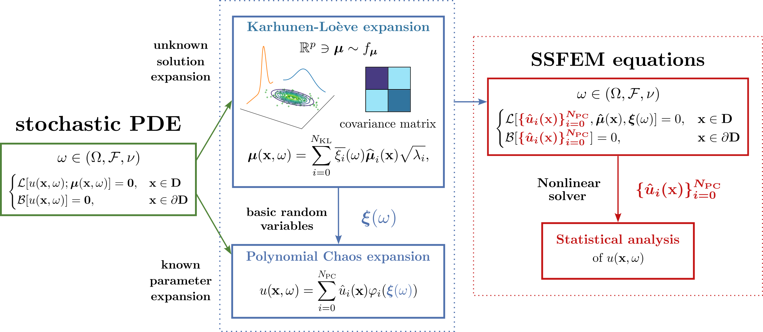
Specifically, we are interested in the capability of the Polynomial Chaos (PC) [50, 58] surrogate model, to obtain accurate information on the branches evolution in the parametric space. To obtain a PC formulation of any stochastic PDEs solution, we considered the Spectral Stochastic Finite Element Method (SSFEM) pipeline [49], which extends the well known FEM projection approach to the probabilistic setting under investigation. Namely, we first model the parameter of the system as a known stochastic processes that can be expanded over the eigenfunctions of the covariance matrix, i.e. the so-called Karhunen-Loève (K-L) expansion. Then, we write the unknowns of the system in the PC form, exploiting the previously computed eigenfunctions as basic random variables. Solving the stochastic PDE now means finding the PC coefficients for the solution, typically via a generic nonlinear solver. Finally, once obtained such representation, a statistical analysis on the solution can be easily performed thanks to the orthogonal properties of the PC polynomials, which enable the computation of the statistical moments through proper combinations of the coefficients themselves. A schematic overview of the developed pipeline is illustrated in Figure 1.

Figure 1. Pipeline for the statistical analysis of bifurcating phenomena via the stochastic-perturbation approach.

Polynomial Chaos has become increasingly prominent in stochastic computation to properly model in the discrete setting the presence of stochastic parameters in PDEs. Indeed, treating pivotal parameters as random variables, PC yields probability density functions (PDFs) linked with the quantities of interest of the system. As such, both the propagation of stochastic terms through the equations and the peculiar properties of the PC expansion furnish insights into the statistical properties of the solution, facilitating its investigation from the statistical standpoint.

In this work, we study the results of SSFEM applied to a specific and well-known bifurcating phenomenon in computational fluid dynamics: the Coandă effect [53, 41]. To increase the complexity of the problem, within this work we consider the viscosity of the fluid as a random variable. Given its role in the bifurcation, this step is fundamental to investigate how its mean and variance influence the velocity field solution.

We focus our analysis on the shape of the polynomial solutions in the probability space while increasing the order of degree of the expansion, and on their statistical moments obtained through the SSFEM approach. Moreover, we discuss a close connection between the numerical expansion of the solution probability distribution and the deterministic bifurcating branches, which up to our knowledge, has not been investigated in literature and could open interesting scenarios.

In order to properly deepen into the topics, we firstly introduce in Section 3 the two expansions used in the SSFEM setting, through which we are able to represent a generic second-order stochastic process in a finite-dimensional space: the K-L and the PC expansions. Moreover, their inclusion in the context of stochastic PDEs is argued, together with a comparison between non-intrusive sample-based and intrusive methods, discussing the problem of retrieving the solution expansion coefficients in the bifurcating setting. Successively, we proceed with the description of the SSFEM intrusive approach in Section 4, finally presenting its application to the specific context of the Navier-Stokes equation for the Coandă effect in Section 5. Therefore, in Section 6 we show the numerical results, underlying the relation discovered between the PC surrogate model of the solution and its deterministic bifurcation diagram.

2. Related works

The study of bifurcating phenomena in nonlinear PDEs has been a subject of extensive research due to its relevance in various physical and engineering domains [2].

Traditional numerical methods [13], including the finite element method [17], finite volume method [59], and spectral element method [39], have been widely employed to explore the coexisting solution branches and the critical regime in a neighborhood of the bifurcation points. Indeed, several numerical techniques are needed to effectively explore or control the global behavior of the system, such as continuation techniques [1, 20] and deflation methods [22]. These tools are respectively designed to reconstruct a specific solution branch, and discover new admissible ones as parameters vary. Additionally, one could also be interested in adopting control strategies on a bifurcation problem, in order to control its behaviour in the parameters space [10].

When dealing with complex problems, the computational effort associated with all these tasks for a complete exploration of the model could be unbearable. Recent works focused on developing reduced-order models (ROMs) [25, 8] to enable many-query simulations, and thus recovering efficiently the full bifurcating pattern. These approaches can be divided in two categories: the ones exploiting standard projection-based techniques [35, 40, 30, 39], and the data-driven ones based on machine-learning strategies [12, 36, 37, 18].

All the above works treat the bifurcation problem in absence of randomness, but such setting is often not physically realistic, even if deterministic assumptions simplify the analysis to explore the contribution of the nonlinearities of the system without additional computational burden. Nevertheless, the presence of stochasticity in the models cannot be disregarded for a comprehensive analysis of the topic, as, in line with other complex problems, bifurcation phenomena face various uncertainties due to input variability, parameter uncertainty, and numerical discretization [45].

Towards a more realistic study of the problem, the concept of deterministic bifurcation has been expanded in the stochastic setting with the analysis of additive and multiplicative noise effects on the models, thus characterizing various types of stochastic bifurcations [4, 6]. Indeed, while in the deterministic case the bifurcation corresponds to a qualitative change in the dynamics of the system as a response to a small variation of the parameters, in the stochastic case it can be observed as a sudden change in some invariant measure of the system. Such changes can involve variations in the largest Lyapunov exponent (dynamical bifurcations), as well as changes in the shape of the solution probability density function (phenomenological bifurcations) [5].

Early investigations explored the dynamic response, stability, and bifurcating behavior of nonlinear dynamical systems under stochastic excitation. In [48], the author studied the impact of small stochastic perturbations on systems exhibiting codimension-one and -two bifurcations. The work exploited methods of stochastic averaging and stochastic normal forms to analyze the asymptotic behavior of nonlinear dynamical systems in the presence of noise. Furthermore, various works have been conducted for specific systems of equations, such as the stochastic reaction-diffusion equation perturbed by an infinite-dimensional Wiener process in [9], and the stochastic regime-switching predator–prey system in [33].

Investigating the interplay between deterministic and stochastic bifurcations, the authors in [34] propose a method to derive probabilistic bifurcation diagrams for stochastic nonlinear dynamical systems using the Fokker-Planck equation.

In [54], the authors explore stochastic bifurcations in Rayleigh–Bénard convection within a two-dimensional cavity. The study investigates the onset of instability, and the existence of multiple stable states under specific ranges of Rayleigh number.

Through stochastic simulations conducted around a point of deterministic bifurcation, the authors reveal the influence of random initial flow states on convection patterns.

The importance of stochastic aspects has been highlighted via Monte Carlo simulations in [43], investigating the probabilities of the solution branches through a stochastic sampling of the parameterized initial conditions. Moreover, they introduce a comparison between the accuracy of statistical moments computation of Monte Carlo sampling and the PC expansion of the solution, confirming the high reliability and computational convenience of the latter.

3. Stochastic modeling in PDEs: stochastic expansions

Given an established deterministic model for a physical system, the question we want to address with this work is related to the definition of a convenient set up for a stochastic model, aiming at studying the effect of uncertainty in the inputs on the system itself.

As illustrated in Figure 1, the starting point of such analysis is the characterization of the random inputs $\bm{\mu}(\bm{x},\omega):\mathcal{D}\times\Omega\rightarrow\mathbb{R}^{p}$ for a stochastic PDE of the form:

(1) $$\begin{cases}\mathcal{L}[u(\bm{x},\omega);\bm{\mu}(\bm{x},\omega)]=0&\quad\bm{x}\in\mathcal{D},\quad\omega\in\Omega,\\ \mathcal{B}[u(\bm{x},\omega)]=0&\quad\bm{x}\in\partial\mathcal{D},\quad\omega\in\Omega,\end{cases}$$

where $\mathcal{L}$ and $\mathcal{B}$ incorporate respectively the physics and the boundary constraints, $u(\bm{x},\omega):\mathcal{D}\times\Omega\rightarrow\mathbb{R}$ is the unknown solution of the system, $\mathcal{D}\subset\mathbb{R}^{n}$ the spatial domain, and $(\Omega,\mathcal{F},\nu)$ a probability space.

By considering the solution as a generic stochastic process $\bm{\alpha}(\bm{x},\omega)$, we need to reduce the infinite-dimensional probability space to a finite-dimensional one to enable numerical computations. This is accomplished by exploiting a decomposition of the stochastic processes space via a finite set of random variables, built with specific stochastic approaches.

We recall that a generic real stochastic process is defined as a family $\bm{\alpha}(\bm{x},\omega)=\{\bm{\alpha}(\bm{x},\cdot)\}_{\bm{x}\in\mathcal{D}}$ of random variables, which are in turn measurable functions of the type $\bm{\alpha}(\bm{x},\cdot):(\Omega,\mathcal{F},\nu)\rightarrow(\mathbb{R}^{d},\mathcal{B})$ for a generic $d<\infty$.

Then, we are interested in obtaining meaningful expansions of the real stochastic processes $\bm{\alpha}(\bm{x},\omega)$ having finite second-order moment, thus belonging to the space:

(2) $$\mathbb{L}_{2}(\Omega,\mathcal{F},\nu;\mathbb{R}^{d}):=\{\bm{\alpha}(\bm{x},\omega):\mathcal{D}\times\Omega\rightarrow\mathbb{R}^{d}\ \quad\text{s.t.}\ \quad\mathbb{E}[\bm{\alpha}^{2}(\bm{x},\cdot)]=\int_{\Omega}\bm{\alpha}(\bm{x},\omega)^{2}d\nu(\omega)<\infty\}.$$

In this section, two well-known methodologies are introduced: the Karhunen-Loève and the Polynomial Chaos expansions, which constitute the basis for the generalization of FEM in the probabilistic context, allowing for the definition of the Spectral Stochastic Finite Element Method, which will be discussed in Section 4.

3.1. Karhunen-Loève expansion

The Karhunen-Loève (K–L) expansion [28, 32, 3] operates similarly to the Fourier expansion but it applies to the space of stochastic processes with finite second-order moment $\mathbb{L}_{2}(\Omega,\mathcal{F},\nu;\mathbb{R}^{d})$. The main idea of the method is to first find the orthonormal eigenfunctions $\bm{\pi}_{i}(\bm{x})$ of the Hilbert-Schmidt integral operator $\mathcal{H}_{K}$ defined as:

(3) $$\mathcal{H}_{K}[\bm{\pi}_{i}(\bm{x})](\bm{x})=\int_{\mathcal{D}}K_{\bm{\alpha}}(\bm{x},\bm{y})\bm{\pi}_{i}(\bm{y})d\bm{y}=\lambda_{i}\bm{\pi}_{i}(\bm{x}),$$

whose kernel $K_{\bm{\alpha}}(\bm{x},\bm{y})$ is the covariance function of the process $\bm{\alpha}(\bm{x},\omega)\in\mathbb{L}_{2}(\Omega,\mathcal{F},\nu;\mathbb{R}^{d})$, and $\lambda_{i}$ are the eigenvalues associated with $\bm{\pi}_{i}(\bm{x})$. Subsequently, the process is projected onto such orthonormal basis, obtaining the random variables:

(4) $$\xi_{i}(\omega)=\int_{\mathcal{D}}\bm{\alpha}(\bm{x},\omega)\bm{\pi}_{i}(\bm{x})d\bm{x}\quad\text{s.t.}\quad\mathbb{E}[\xi_{i}]=0,\ \text{and}\ \mathbb{E}[\xi_{i}\xi_{j}]=\lambda_{i}\delta_{i,j},$$

where the conditions on their mean and variance are easily obtained substituting the $\bm{\pi}_{i}(\bm{x})$ functions with their definition in Equation (3). Namely, they are orthogonal in $\mathbb{L}_{2}(\Omega,\mathcal{F},\nu;\mathbb{R}^{d})$, thus uncorrelated. The K-L expansion can then be expressed as:

(5) $$\begin{split}\bm{\alpha}(\bm{x},\omega)&=\overline{\bm{\alpha}}(\bm{x})+\sum_{i=1}^{\infty}\frac{\xi_{i}(\omega)}{\sqrt{\lambda_{i}}}\bm{\pi}_{i}(\bm{x})\sqrt{\lambda_{i}}\\ &=\overline{\bm{\alpha}}(\bm{x})+\sum_{i=1}^{\infty}\overline{\xi_{i}}(\omega)\bm{\pi}_{i}(\bm{x})\sqrt{\lambda_{i}}\\ &=\sum_{i=0}^{\infty}\overline{\xi_{i}}(\omega)\bm{\pi}_{i}(\bm{x})\sqrt{\lambda_{i}},\end{split}$$

where the first two equivalence follow directly from introducing the normalized random variables $\overline{\xi_{i}}(\omega)$ such that $\mathbb{E}[\overline{\xi_{i}}]=0$ and $\mathbb{E}[\overline{\xi_{i}}\overline{\xi_{j}}]=\delta_{i,j}$, and assuming without loss of generality that $\overline{\xi_{0}}(\omega)\sim\mathcal{N}(1,0)$, $\bm{\pi}_{0}(\bm{x})=\overline{\bm{\alpha}}(\bm{x})$, and $\lambda_{0}=1$.

The convergence properties of this expansion clearly strictly depend on the nature of the stochastic process covariance function, namely on the decay of its eigenvalues. For a further discussion on the topic we refer to [26].

In general, it is to be noted that the K-L expansion is particularly useful to model the parameters of a generic stochastic PDE (1), since their covariance function is known and all the computation comes down to its spectral study.

3.2. Polynomial Chaos expansion

The PC expansion [55, 23] decomposes a stochastic process $\bm{\alpha}(\bm{x},\omega)\in\mathbb{L}_{2}(\Omega,\mathcal{F},\nu;\mathbb{R}^{d})$ thanks to the Cameron-Martin theorem [14].

This theorem establishes the existence of a sequence of closed, pairwise orthogonal linear subspaces of $\mathbb{L}_{2}(\Omega,\mathcal{F},\nu;\mathbb{R}^{d})$ which are spanned by polynomial bases. In particular, the PC expansion can be exploited to express the process $\bm{\alpha}(\mathbf{x},\omega)$ as the infinite sum:

(6) $$\bm{\alpha}(\mathbf{x},\omega)=\sum_{i=0}^{\infty}\widehat{\bm{\alpha}}_{\bm{i}}(\mathbf{x})\psi_{i}(\{\zeta_{j}(\omega)\}_{j=1}^{N_{\text{RV}}}),$$

where $\widehat{\bm{\alpha}}_{\bm{i}}(\mathbf{x})$ are the expansion coefficients associated with the stochastic basis $\psi_{i}(\{\zeta_{j}(\omega)\}_{j=1}^{N_{\text{RV}}}):(\Omega,\mathcal{F},\nu)\rightarrow\mathbb{R}$, which are instead the set of polynomial basis orthogonal with respect to the Gaussian measure $d\nu_{\bm{\zeta}}$ and depending on $N_{RV}$ independent standard normal random variables $\zeta_{j}(\omega)$. Namely:

(7) $$\int_{\mathbb{R}^{d}}\psi_{i}(\bm{\zeta})\psi_{j}(\bm{\zeta})d\nu_{\bm{\zeta}}\ =\ \parallel\psi_{i}\parallel^{2}\delta_{i,j},$$

where we have indicated the set of random variables, called also seeds or basic random variables, as $\bm{\zeta}=\{\zeta_{j}(\omega)\}_{i=1}^{N_{\text{RV}}}$ .

For computational purposes, the infinite sum in (6) is truncated to a finite number of terms $N_{PC}$. It is often useful to relate such number to the desired maximum degree $M$ of the polynomials, and the number or variables $N_{RV}$ from which they depend, so that the following formula can easily be proved through combinatorial calculus:

(8) $$1+N_{PC}=\frac{(M+N_{RV})!}{M!N_{RV}!}.$$

A generalization of this result has been presented in [57] with the generalized Polynomial Chaos (gPC), in which the PC expansion is obtained using different classes of polynomials, depending on the measure associated to the basic random variables $\bm{\zeta}$. Such polynomials, also known as Wiener-Askey polynomials, are classified in the Askey-scheme that we partially report in Table 1. Convergence of moments, convergence in probability, and convergence in law have been proved for such expansions; for a more in-depth discussion, we refer the reader to [27, 21].

Type	Basic random variables	Wiener-Askey polynomials	Support
Continuous	Gaussian	Hermite	$(-\infty,\infty)$
	Gamma	Laguerre	$[0,\infty)$
	Beta	Jacobi	$[a,b]$
	Uniform	Legendre	$[a,b]$
Discrete	Poisson	Charlier	$\{0,1,2,\dots\}$
	Binomial	Krautchouk	$\{0,1,2,\dots,N\}$
	Negative Binomial	Meixner	$\{0,1,2,\dots\}$

Table 1. Some of the correspondences between basic random variables, the Wiener–Askey orthogonal polynomials for gPC expansion, and their support.

3.3. Intrusive and non-intrusive approaches

In the former sections, we have seen that modeling the stochastic components of the system as random variables and stochastic processes allows us to express them as series expansions. However, a crucial task in this context consists in the determination of the coefficients for such representation when the covariance function is unknown. Furthermore, once found their representation, such expansions could also be used to infer relevant statistical information, such as statistical moments.

In general, when well-established deterministic codes exist, sample–based non–intrusive stochastic simulations of the system can be [7] performed repeating the same solution computation for different parameters values. Such methods include Monte Carlo simulation [43], orthogonal spectral projection [56], and stochastic collocation [7]. Monte Carlo simulation gathers a set of solutions by varying input parameters and then deduces statistical properties from the collected data. On the other hand, orthogonal spectral projection aims at determining solution expansion coefficients through numerical integration of its projection integral, while stochastic collocation achieves this through interpolation of sampled deterministic solutions. For a more thorough discussion, we refer the interested reader to [51].

However, in the context of bifurcating behavior, sample–based approaches may not be suitable. Indeed, as we will point out in Section 5.1, deterministic numerical solvers provide results strictly dependent on the given initial guess, often guiding the final solution to a specific branch among all possible ones. Because of this limitation, obtaining reliable statistical information on the solution using such methods is quite complex and not completely meaningful. Thus, such scenarios need the development of intrusive approaches which are independent on the availability of solution samples.

Towards this goal, in the next section we introduce an intrusive intrusive way of retrieving the unknown coefficients of the PC expansion of the solution.

4. Spectral Stochastic Finite Element Method

In this section we rewrite in the form shown in (9) the general framework of a stochastic PDE already presented in Equation (1), and describe the SSFEM pipeline explaining how the two stochastic expansions introduced before can be connected in order to obtain a PC expansion of the solution.

Let $\mathcal{D}\subset\mathbb{R}^{n}$ ($n=2,3$) represent a bounded domain, and $(\Omega,\mathcal{F},\nu)$ denote a probability. We consider the following general abstract problem:

(9) $$(\bm{D}(\bm{x})+\bm{S}(\bm{x},\bm{\mu}(\bm{x},\omega)))[u(\bm{x},\omega)]=\bm{f}(\bm{x})\ \quad\text{for}\ \bm{x}\in\mathcal{D},\ \omega\in\Omega$$

where $u(\bm{x},\omega):\mathcal{D}\times\Omega\rightarrow\mathbb{R}$ is the unknown function, and $\bm{\mu}(\bm{x},\omega):\mathcal{D}\times\Omega\rightarrow\mathbb{R}^{p}$ represents the $p$-dimensional stochastic process characterizing the system’s parameters. The deterministic operator $\bm{D}$ and its stochastic counterpart $\bm{S}$ act on $u(\bm{x},\omega)$ returning an object that belongs to $\mathbb{R}^{out}$, while $\bm{f}(\bm{x}):\mathcal{D}\rightarrow\mathbb{R}^{out}$ represents the source term.

Figure 2. Synthetic workflow diagram showing the process of computing the corresponding PDF of $u(\bm{x},\omega)$ by solving Equation (9) using SSFEM.

The general workflow we are interested in, reported in a synthetic version in Figure 2, starts with an arbitrary and known covariance function assigned to $\bm{\mu}$, which is taken to be a stochastic process with finite second-order moments. The final goal is the computation of the corresponding probability density function (PDF) for $u$ by exploiting Equation (9), and the analysis of meaningful statistics. For this purpose the SSFEM has been adopted, as it provides a natural extension of FEM enhanced with the notion of stochastic process expansions through an orthogonal decomposition of the space $\mathbb{L}_{2}(\Omega,\mathcal{F},\nu;\mathbb{R})$.

In particular, the stochastic parameters are expanded using the K-L decomposition presented in Section 3.1: considering the stochastic process $\bm{\mu}$ with a known covariance function $K_{\bm{\mu}}(\bm{x},\bm{y})$, the decomposition performs a separation of stochastic and deterministic variables:

(10) $$\bm{\mu}(\bm{x},\omega)=\sum_{i=0}^{N_{\text{KL}}}\overline{\xi_{i}}(\omega)\widehat{\bm{\mu}}_{i}(\bm{x})\sqrt{\lambda_{i}},$$

where we denoted by $\widehat{\bm{\mu}}_{i}(\bm{x})$ the eigenfunctions of $K_{\bm{\mu}}(\bm{x},\bm{y})$.

It is important to remark that a direct and straightforward K-L expansion of the solution $u$ is not feasible since the covariance function of the solution process is not known a-priori. Therefore, the representation of $u$ is achieved via the gPC expansion (Section 3.2), consisting of a truncated series comprising of the first $N_{\text{PC}}$ terms:

(11) $$u(\bm{x},\omega)=\sum_{i=0}^{N_{\text{PC}}}\widehat{u}_{i}(\bm{x})\psi_{i}(\{\overline{\xi_{l}}(\omega)\}_{l=1}^{N_{\text{KL}}}),$$

where we used as the $\{\zeta_{j}(\omega)\}_{j=1}^{N_{\text{RV}}}$ of equation (6), the uncorrelated normalized random variables $\{\overline{\xi_{j}}(\omega)\}_{j=1}^{N_{\text{KL}}}=:\bm{\xi}(\omega)$ resulting from the K-L expansion of the parameters.

For the sake of simplicity, let us consider the case where $p=1$ and the stochastic operator $\bm{S}$ in Equation $\eqref{eq:general_prob}$ can be decomposed as $\bm{S}(\mu,\bm{x})=\mu\bm{S}(\bm{x})$. By inserting the formulation of the gPC and the K-L expansions, respectively for $u$ and $\mu$, into Equation (9), we can rewrite the problem as follows:

(12) $$\left(\bm{D}(\bm{x})+\sum_{i=0}^{N_{\text{KL}}}\overline{\xi_{i}}(\omega)\widehat{\mu}_{i}(\bm{x})\sqrt{\lambda_{i}}\bm{S}(\bm{x})\right)\left[\sum_{j=0}^{N_{\text{PC}}}\widehat{u}_{j}(\bm{x})\psi_{j}(\bm{\xi}(\omega))\right]=\bm{f}(\bm{x}).$$

Once that the stochastic nature of the problem has been tackled, we can now numerically approximate the formulation above through a classical FEM. This involves performing a Galerkin projection on the subspace $\mathcal{D}_{h}\subset\mathcal{D}$ spanned by a set of deterministic basis functions $\{\phi_{k}(\bm{x})\}_{k=1}^{N_{\text{D}}}$. By doing this, we can expand each gPC coefficient with respect to the FEM basis as:

(13) $$\widehat{u}_{j}(\bm{x})=\sum_{k=1}^{N_{D}}\widehat{u}_{k,j}\phi_{k}(\bm{x}),\quad\forall j\in\{0,\dots,N_{\text{PC}}\}.$$

Substituting the former expansion into Equation (12), we obtain the formulation:

(14) $$\left(\bm{D}(\bm{x})+\sum_{i=0}^{N_{\text{KL}}}\overline{\xi_{i}}(\omega)\widehat{\mu}_{i}(\bm{x})\sqrt{\lambda_{i}}\bm{S}(\bm{x})\right)\left[\sum_{j=0}^{N_{\text{PC}}}\sum_{k=1}^{N_{D}}\widehat{u}_{k,j}\phi_{k}(\bm{x})\psi_{j}(\bm{\xi}(\omega))\right]=\bm{f}(\bm{x}),$$

that has to be solved for the unknown $\mathbf{\widehat{U}}={\{\widehat{u}_{k,j}\}_{k=1}^{N_{D}}}{\vphantom{=\{\widehat{u}_{k,j}\}}}_{j=0}^{N_{\text{PC}}}\in\mathbb{R}^{N_{\text{D}}\times(N_{\text{PC}}+1)}$.

To construct an algebraic system of equations for $\mathbf{\widehat{U}}$ one imposes the orthogonality of the residual in Equation (14) with respect to the deterministic and stochastic test functions, respectively $\{\phi_{n}(\bm{x})\}_{n=1}^{N_{\text{KL}}}$ and $\{\psi_{m}(\bm{\xi})\}_{m=0}^{N_{\text{PC}}}$.

The discrete counterpart of the stochastic PDE now reads as the system of equations:

(15) $$\begin{split}&\sum_{j=0}^{N_{\text{PC}}}\sum_{k=1}^{N_{D}}C_{j,m}\widehat{u}_{k,j}A_{k,n}+\sum_{i=0}^{N_{\text{KL}}}\sum_{j=0}^{N_{\text{PC}}}\sum_{k=1}^{N_{D}}E_{i,j,m}\widehat{u}_{k,j}B_{i,k,n}=F_{n},\\ &\hskip 216.81pt\forall n\in\{1,\dots,N_{D}\},\forall m\in\{0,\dots,N_{\text{PC}}\},\end{split}$$

where we have introduced the following notation for the coefficients of the tensors to be assembled:

(16a) $$A_{k,n} =\int_{\mathcal{D}}\bm{D}(\bm{x})[\phi_{k}(\bm{x})]\phi_{n}(\bm{x})d\bm{x},$$

(16b) $$B_{i,k,n} =\int_{\mathcal{D}}\widehat{\mu_{i}}(\bm{x})\bm{S}(\bm{x})[\phi_{k}(\bm{x})]\phi_{n}(\bm{x})d\bm{x},$$

(16c) $$F_{n} =\int_{\mathcal{D}}\bm{f}(\bm{x})\phi_{n}(\bm{x})d\bm{x},$$

(17a) $$C_{j,m} =\int_{\mathbb{R}^{d}}\psi_{j}(\bm{\xi})\psi_{m}(\bm{\xi})d\nu_{\bm{\xi}},$$

(17b) $$E_{i,j,m} =\int_{\mathbb{R}^{d}}\overline{\xi_{i}}\sqrt{\lambda_{i}}\psi_{j}(\bm{\xi})\psi_{m}(\bm{\xi})d\nu_{\bm{\xi}}.$$

Therefore, the system can now be solved in function of the unknown $\widehat{\bm{U}}$ with a generic nonlinear solver, assuming a generic nonlinear nature of the two operators $\bm{D}$ and $\bm{S}$. As it will be underlined in the results section, the choice of the solver represents a crucial choice for the methodology. Indeed, when interested in simulations involving dense grids (i.e. high $N_{\text{D}}$), and high polynomial degrees (i.e. high $N_{\text{PC}}$), the convergence rate of the solver might be compromised by the cardinality of the degrees of freedom of $\widehat{\bm{U}}$.

4.1. Statistical moments computation

A significant advantage of the gPC representation is that, having obtained the solution coefficients $\widehat{\bm{U}}$ from Equation (15), it enables an easy computation of the first and second-order moments of the solution probability distribution.

Indeed, leveraging the orthogonality property of the polynomials $\{\psi_{i}\}_{i=1}^{N_{\text{PC}}}$, and recognizing that, since the polynomial of degree zero is constant, the following condition holds:

(18) $$\mathbb{E}[\psi_{i}(\bm{\xi})]=\mathbb{E}[\psi_{i}(\bm{\xi})\psi_{0}(\bm{\xi})]=\delta_{i,0}\quad\forall i\in\{0,\dots,N_{\text{PC}}\},$$

it can be observed that the mean of the solution is equivalent to the first coefficient of the expansion:

(19) $$\mathbb{E}[u(\omega,\bm{x})]=\mathbb{E}\left[\sum_{i=0}^{N_{\text{PC}}}\widehat{u}_{i}(\bm{x})\psi_{i}(\bm{\xi})\right]=\widehat{u_{0}}(\bm{x}).\\$$

Furthermore, each element of the covariance matrix can be approximated by a weighted sum involving the products of all the coefficients except the first one $\widehat{u_{0}}$, where the weights correspond to the polynomial stochastic norms $\mathbb{E}[\bm{\psi}_{i}^{2}]$:

(20) $$\begin{split}\mathrm{Cov}\left[u(\omega,\bm{x}),u(\omega,\bm{x})\right]&=\mathbb{E}\left[\left(\sum_{i=0}^{N_{\text{PC}}}\widehat{u_{i}}(\bm{x})\psi_{i}(\bm{\xi})-\widehat{u_{0}}(\bm{x})\right)\left(\sum_{i=0}^{N_{\text{PC}}}\widehat{u_{i}}(\bm{y})\psi_{i}(\bm{\xi})-\widehat{u_{0}}(\bm{y})\right)\right]\\ &=\sum_{i=1}^{N_{\text{PC}}}\widehat{u_{i}}(\bm{x})\widehat{u_{i}}(\bm{y})\mathbb{E}[\bm{\psi}_{i}^{2}].\end{split}$$

The straightforward computation of the statistical moments from the PC surrogate model represents a key advantage for the implementation of the SSFEM pipeline. Indeed, within the PC context, the PDF reconstruction is facilitated by the both the moments computation, through a proper combination of the coefficients, and the sampling of the solution probability distribution, achieved evaluating the solution polynomials at a sample of their basic random variables $\bm{\xi}$.

5. A revisited benchmark in fluid-dynamics: the Coandă effect

Let $\mathcal{D}\in\mathbb{R}^{2}$ be the bounded domain representing a sudden-expansion channel in Figure 3.

Figure 3. Computational domain representing the two-dimensional sudden-expansion channel.

We consider the steady incompressible Navier–Stokes equations described by the PDE system:

(21) $$\begin{cases}-\mu\Delta\bm{v}+\bm{v}\cdot\nabla\bm{v}+\nabla p=0&\text{in}\ \ \mathcal{D},\\ \bm{\nabla}\cdot\bm{v}=0&\text{in}\ \ \mathcal{D},\\ \end{cases}$$

where the unknown state of the fluid, defined by $(\bm{v},p)$, encompasses its velocity $\bm{v}=(v_{1},v_{2})$ and pressure $p$ normalized over a constant density.

The parameter $\mu$ represents the kinematic viscosity, and plays a fundamental role in the behavior of the system. Indeed, being related to the Reynolds number, balancing the viscous and inertial forces, it originates a symmetry-breaking phenomenon, known as the Coandă effect. The unique stable symmetric branch bifurcates in two asymmetric coexisting configurations, switching its stability property with them at critical values of the fluid’s viscosity parameter, generating a pitchfork bifurcation. Its study has relevance in various fields of application, ranging from shape-modeling in aerodynamics to cardiovascular blood-flow in health-care, recently garnering a substantial body of literature, comprising both experimental and deterministic numerical investigations [46, 16, 53, 38, 11, 29]. In particular, it models the “wall-hugging” tendency of a viscous fluid, which for instance in the cardiovascular setting could cause mitral valve [38].

The imposed boundary conditions for the Navier–Stokes problem (21) are the following:

(22) $$\begin{cases}\bm{v}=\bm{v}_{\text{in}}&\text{on}\ \ \Gamma_{\text{in}},\\ \bm{v}=0&\text{on}\ \ \Gamma_{\text{wall}},\\ -p\bm{n}+(\mu\nabla\bm{v})\bm{n}=0&\text{on}\ \ \Gamma_{\text{out}},\\ \end{cases}\quad\text{with}\quad\bm{v}_{\text{in}}(x_{1},x_{2})=\begin{bmatrix}20(5-x_{2})(x_{2}-2.5)\\ 0\\ \end{bmatrix},$$

entailing: a stress-free boundary condition on the velocity at the outlet $\Gamma_{\text{out}}$, with the outer normal denoted as $\bm{n}=(n_{x_{1}},n_{x_{2}})$; a no-slip homogeneous Dirichlet boundary condition on $\Gamma_{\text{wall}}$; and a non-homogeneous Dirichlet boundary condition $\bm{v}_{\text{in}}$ at the inlet $\Gamma_{\text{in}}$. For more details regarding the benchmark we refer the reader to [38].

For the numerical approximation of the problem, we first need to consider its weak formulation, that reads as: given a parameter $\mu\in\mathcal{P}$ , find $(\bm{v},p)\in\mathbb{V}_{\text{in}}\times\mathbb{Q}$ such that

(23) $$\begin{cases}\mu\int_{\mathcal{D}}\nabla\bm{v}\cdot\nabla\bm{\psi}d\bm{x}+\int_{\mathcal{D}}(\bm{v}\cdot\nabla\bm{v})\bm{\psi}d\bm{x}-\int_{\mathcal{D}}p\nabla\cdot\bm{\psi}d\bm{x},\quad&\forall\bm{\psi}\in\mathbb{V}_{0}\\ +\int_{\mathcal{D}}\pi\nabla\cdot\bm{v}d\bm{x}=0,\quad&\forall\pi\in\mathbb{Q},\end{cases}$$

where we have defined the continuous function spaces as:

$$\mathbb{V}_{0} =\left\{\bm{v}\in H^{1}\left(\mathcal{D};\mathbb{R}^{2}\right):\left.\bm{\psi}\right|_{\Gamma_{\text{wall}}\cup\Gamma_{\text{in}}}=0\right\},$$

$$\mathbb{V}_{\text{in}} =\mathbb{V}_{0}\oplus\bm{v}_{\text{in}}$$

$$\mathbb{Q} =L^{2}(\mathcal{D}).$$

In the next sections, we exploit the weak formulation derived in (23) to recover the bifurcation diagram, both in the deterministic setting and using a non-intrusive Monte Carlo sampling. Finally, we present the details of the SSFEM pipeline, specific for the benchmark under investigation, in order to study the properties and results of the perturbation approach in the stochastic setting.

5.1. Deterministic bifurcation analysis

The pitchfork bifurcation originating from the Navier–Stokes system in (21) with boundary conditions reported in (22) has been deeply investigated in literature in the deterministic setting, where the kinematic viscosity $\mu$ plays the role of the bifurcation parameter, causing the fluid to adhere to adjacent walls.

Specifically, when studying the behavior of the solution to the system in (21), while decreasing the kinematic viscosity, the influence of inertia gradually becomes more significant, leading to a breakdown of solution symmetry at a critical viscosity value, denoted as $\mu^{*}$.

Therefore, below this critical threshold, the uniqueness of the solution is lost, and we expect to observe a physically unstable symmetrical flow configuration alongside two stable asymmetric solutions that display wall-hugging behavior. Notably, these solutions coexist for the same parameter values, a characteristic feature of these kind of bifurcating phenomena.

Figure 4. Deterministic FEM bifurcation diagram with the corresponding co-existing solutions belonging to the upper, middle and lower branches for $\mu=0.5$.

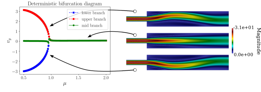
To build a bifurcation diagram for the Coandă problem, and thus investigate the evolution of all the solution branches, one may choose to examine the behavior of the vertical velocity, the component responsible for breaking the symmetry, at a point along the channel’s symmetry axis $\widehat{x}$, as illustrated in Figure 4. To construct such deterministic diagram, giving a visual information regarding the model’s behavior, one needs an iterative process involving the solution of the problem in (21) with some high-fidelity numerical solver. The parameter $\mu$ has been considered as a known parameter, varying uniformly in the parametric space $\mathbb{P}=[0.5,2]$, with a step size $\Delta\mu=0.01$. The strategy to recover the plot in Figure 4 is complex and costly, involving a continuation strategy to properly select the initial guess for the nonlinear solver. Consistently with the results in literature we can see that, within this parametric/geometry context, the bifurcation occurs at a value of the parameter $\mu^{*}\approx 0.96$. Thus, in the well-known deterministic setting the fixed location of the bifurcation points allows for several computational simplifications, but towards a more realistic and complex scenario it is important to study the properties of the branching behavior in a stochastic setting.

5.2. A non–intrusive approach: Monte Carlo sampling

As anticipated in Section 3.3, a sample–based approach to bifurcation problems could be misleading, providing only partial information about the system’s behavior when any a-priori assumption on the potential multiplicity of the existing branches is made. Indeed, without exploiting ad-hoc techniques such as the deflation method [22], the are no guarantees that the nonlinear solver is able to find samples of the solution equally distributed on the possible branches.For instance, approaching the problem via MC simulations, or similar non–intrusive methodologies, one collects an ensemble of solutions by repeatedly solving the system for different values of the stochastic parameters.

Therefore, as a first step in the stochastic context, we investigate the Navier–Stokes system treating the viscosity as a normally distributed random variable $\mu\sim\mathcal{N}(0.9,0.001)$ centered at the point $0.9$, where the bifurcation has already occurred. In order to validate the assumptions made in Section 3.3, we draw $300$ samples from such parameter distribution and solve the nonlinear system for these values, collecting an ensemble of solutions.

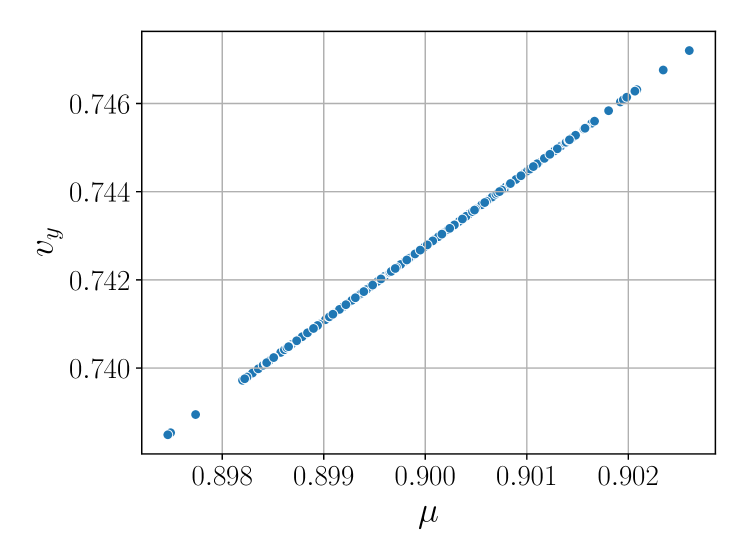
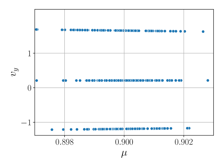
As shown in Figure 5(a), if the nonlinear solver initialization is not exploiting any prior knowledge regarding the possible states, but it is set to zero, the variance obtained from the collected ensemble has small magnitude in the whole domain. On the other hand, if we incorporate some knowledge by means of a random continuation approach for the initialization of the Newton–Krylov method, the variance clearly shows a different behavior with an increased magnitude, and concentrates in the expansion-region of the channel, as it can be seen in Figure 5(b).

(a) Fixed initialization of the numerical solver to a null vector.

(b) Ad-hoc initialization of the numerical solver basing on a prior knowledge of the solutions branches.

Figure 5. Variance of the vertical component of the velocity field solution computed through a MC simulation of $300$ samples with $\mu\sim\mathcal{N}(0.9,0.001)$.

As a further confirmation of the need for additional knowledge in the non–intrusive approach, we can study the actual samples from the grid points realizing the maximum value of the variance in both cases. In Figure 6(a), we see that the higher variance only comes from a linear trend, while in Figure 6(b), corresponding to the ad-hoc initialization of the solver, we observe a multi-valued map identifying the three co-existing branches in the deterministic bifurcation diagram in Figure 4.

(a) Samples of the solution at the point of maximum variance in the case of Figure 5(a).

(b) Samples of the solution at the point of maximum variance in the case of Figure 5(b).

Figure 6. Monte Carlo samples of the vertical component of the velocity field in case of $\mu\sim\mathcal{N}(0.9,0.001)$.

Thus, even if sample–based approaches could be of easier interpretation and implementation, they lack of reliability in case of non–uniqueness of the solution, and require some computationally expensive continuation methods. On the other hand, performing a sample–based stochastic simulation enlarging the parameter interval of interest could lead to interesting results.

It is the case of Figure 7, where we assign greater variance to the parameter and perform the MC non–intrusive method with prior knowledge of the three admissible branches. Indeed, in the case of $\mu\sim\mathcal{N}(0.9,0.2)$, even if the non–sequential analysis of the branches produces less precise solutions of the ones in Figure 4, not only the bifurcation diagram topology is reproduced, but an additional bifurcating behaviour is observed around $\mu=0.5$.

Figure 7. Bifurcation plot in case of $\mu\sim\mathcal{N}(0.9,0.2)$ at the point of maximum variance.

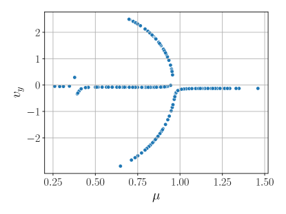
Therefore, sample–based approaches to bifurcating problems do not guarantee an accurate prediction of the complete solution manifold, nonetheless they could serve as interesting starting points for some further analysis, for instance regarding new possible branches. For further investigation on the non–intrusive potentiality in the bifurcating setting, we refer to [52], where the authors analyse such methods in the case of compressible Navier Stokes equations.

However, in this work we are interested in the numerical capabilities of accurately inferring information on the deterministic bifurcation diagram given no prior knowledge of the solution manifold. Following this path, we continue in the next section with the application of the SSFEM intrusive approach to the Navier–Stokes equations with randomic viscosity.

5.3. SSFEM approach: random viscosity parameter

Having highlighted the issues when dealing with non-intrusive approaches, we proceed exploring the evolution of the system via the SSFEM pipeline presented in Section 4. In order to study the behaviour of the solution in a small neighborhood of the viscosity parameter, we consider $\mu$ as the random variable following a Gaussian distribution with mean $\overline{\mu}$ and variance $\sigma^{2}$. This way, we can write its K-L expansion (5) as

(24) $$\mu=\overline{\mu}+\sigma\overline{\xi},$$

where $\pi_{1}(\bm{x})=1$, $\overline{\xi_{1}}=\overline{\xi}\sim\mathcal{N}(0,1)$ and $\lambda_{1}=\sigma^{2}$.

Thus, by expanding the unknowns of the problem in (23) we can write:

(25) $$\bm{v}(\bm{x},\omega)=\sum_{i=0}^{N_{PC}^{\bm{v}}}\sum_{j=1}^{N_{D}^{\bm{v}}}\bm{v}_{j,i}\phi_{j}^{\bm{v}}(\bm{x})\psi_{i}^{\bm{v}}(\bm{\xi}(\omega)),\quad\text{and}\quad p(\bm{x},\omega)=\sum_{i=0}^{N_{PC}^{p}}\sum_{j=1}^{N_{D}^{p}}p_{j,i}\phi_{j}^{p}(\bm{x})\psi_{i}^{p}(\bm{\xi}(\omega)).$$

where we introduced the superscripts to refer to the quantities related to the velocity and pressure fields. This way, the system can be expressed in the generic form of Equation (15). In particular, the first equation in the weak formulation (23) can be expanded both in the FEM space via the test functions $\{\phi_{n}^{\bm{v}}(\bm{x})\}_{n=1}^{N_{D}^{\bm{v}}}$, $\{\phi_{n}^{p}(\bm{x})\}_{n=1}^{N_{D}^{p}}$, and in the probabilistic one with $\{\psi_{m}^{\bm{v}}(\xi)\}_{m=1}^{N_{PC}^{\bm{v}}}$, $\{\psi_{m}^{p}(\bm{\xi})\}_{m=1}^{N_{PC}^{p}}$, as follows:

(26) $$\begin{split}&\sum_{k=0}^{1}\sum_{i=0}^{N_{PC}^{\bm{v}}}\sum_{j=1}^{N_{D}^{\bm{v}}}\bm{v}_{i,j}\int_{\mathbb{R}}\sqrt{\lambda_{k}}\xi_{k}\psi_{i}^{\bm{v}}(\bm{\xi})\psi_{m}^{(\bm{v})}(\bm{\xi})d\nu_{\bm{\xi}}\int_{\bm{D}}\nabla\phi_{j}^{\bm{v}}(\bm{x})\cdot\nabla\phi_{n}^{\bm{v}}(\bm{x})d\bm{x}\\ &+\sum_{i=0}^{N_{PC}^{\bm{v}}}\sum_{j=1}^{N_{D}^{\bm{v}}}\sum_{l=0}^{N_{PC}^{\bm{v}}}\sum_{h=1}^{N_{D}^{\bm{v}}}\bm{v}_{i,j}\bm{v}_{l,h}\int_{\mathbb{R}}\psi_{i}^{\bm{v}}(\bm{\xi})\psi_{l}^{\bm{v}}(\bm{\xi})\psi_{m}^{\bm{v}}(\bm{\xi})d\nu_{\bm{\xi}}\int_{\bm{D}}(\phi_{j}^{\bm{v}}(\bm{x})\cdot\nabla\phi_{h}^{\bm{v}}(\bm{x}))\phi_{n}^{\bm{v}}(\bm{x})d\bm{x}\\ &-\sum_{i=0}^{N_{PC}^{p}}\sum_{j=1}^{N_{D}^{p}}p_{i,j}\int_{\mathbb{R}}\psi_{i}^{p}(\bm{\xi})\psi_{m}^{\bm{v}}(\bm{\xi})d\nu_{\bm{\xi}}\int_{\bm{D}}\phi_{j}^{p}(\bm{x})\nabla\cdot\phi_{n}^{\bm{v}}(\bm{x})d\bm{x}=0,\\ &\hskip 216.81pt\forall n\in\{1,\dots,N_{D}^{\bm{v}}\},m\in\{1,\dots,N_{PC}^{\bm{v}}\}.\end{split}$$

Similarly, one can use the deterministic and probabilistic basis function to expand the second equation in (23), obtaining

(27) $$\begin{split}&\sum_{i=0}^{N_{PC}^{\bm{v}}}\sum_{j=1}^{N_{D}^{\bm{v}}}\bm{v}_{i,j}\int_{\bm{D}}\nabla\cdot\phi_{j}^{\bm{v}}(\bm{x})\phi_{n}^{p}(\bm{x})d\bm{x}\int_{\mathbb{R}}\psi^{\bm{v}}_{i}(\bm{\xi})\psi^{p}_{m}(\bm{\xi})d\nu_{\bm{\xi}}=0,\\ &\hskip 216.81pt\forall n\in\{1,\dots,N_{D}^{p}\},m\in\{1,\dots,N_{PC}^{p}\}.\end{split}$$

We remark that, after the SSFEM expansion, we can write the derived discrete approximation of the weak formulation (23) in the more compact form

(28) $$\begin{cases}\bm{A}^{T}\cdot\bm{U}\cdot(\bm{E}^{(0)}+\bm{E}^{(1)})+\bm{I}-\bm{C}^{T}\cdot\bm{Q}\cdot\bm{G}=\bm{0},\\ \bm{D}^{T}\cdot\bm{U}\cdot\bm{H}=\bm{0}.\end{cases}$$

where we denoted with $\bm{U}\in\mathbb{R}^{N_{D}^{\bm{v}}\times N_{PC}^{\bm{v}}}$ and $\bm{Q}\in\mathbb{R}^{N_{D}^{p}\times N_{PC}^{p}}$, respectively, the unknown coefficients for the velocity and pressure fields, and the FEM and stochastic matrices, respectively in Equations (29) and (30), as

(29a) $$A_{j,n} =\int_{\bm{D}}\nabla\phi_{j}^{\bm{v}}(\bm{x})\cdot\nabla\phi_{n}^{\bm{v}}(\bm{x})d\bm{x},$$

(29b) $$B_{n,j,h} =\int_{\bm{D}}(\phi_{j}^{\bm{v}}(\bm{x})\cdot\nabla\phi_{h}^{\bm{v}}(\bm{x}))\phi_{n}^{\bm{v}}(\bm{x})d\bm{x},$$

(29c) $$C_{j,n} =\int_{\bm{D}}\phi_{j}^{p}(\bm{x})\nabla\cdot\phi_{n}^{\bm{v}}(\bm{x})d\bm{x},$$

(29d) $$D_{j,n} =\int_{\bm{D}}\nabla\cdot\phi_{j}^{\bm{v}}(\bm{x})\phi_{n}^{p}(\bm{x})d\bm{x},$$

(29e) $$I_{n,m} =(\bm{U}^{T}\cdot\bm{B}_{n}\cdot\bm{U})\odot\bm{F}_{m},$$

(30a) $$E_{i,m}^{(0)} =\int_{\mathbb{R}}\sqrt{\lambda_{0}}\xi_{0}\psi_{i}^{\bm{v}}(\bm{\xi})\psi_{m}^{\bm{v}}(\bm{\xi})d\nu_{\bm{\xi}},$$

(30b) $$E_{i,m}^{(1)} =\int_{\mathbb{R}}\sqrt{\lambda_{1}}\xi_{1}\psi_{i}^{\bm{v}}(\bm{\xi})\psi_{m}^{\bm{v}}(\bm{\xi})d\nu_{\bm{\xi}},$$

(30c) $$F_{m,l,i} =\int_{\mathbb{R}}\psi_{i}^{\bm{v}}(\bm{\xi})\psi_{l}^{\bm{v}}(\bm{\xi})\psi_{m}^{\bm{v}}(\bm{\xi})d\nu_{\bm{\xi}},$$

(30d) $$G_{i,m} =\int_{\mathbb{R}}\psi_{i}^{p}(\bm{\xi})\psi_{m}^{\bm{v}}(\bm{\xi})d\nu_{\bm{\xi}},$$

(30e) $$H_{i,m} =\int_{\mathbb{R}}\psi^{\bm{v}}_{i}(\bm{\xi})\psi^{p}_{m}(\bm{\xi})d\nu_{\bm{\xi}},$$

where $\odot$ stands for the Hadamard product.

As concerns the imposition of the boundary conditions defined in the general formulation of the problem (21), we identify the inlet/wall nodes belonging to $\Gamma_{\text{in}}$ and $\Gamma_{\text{wall}}$, and we enforce them strongly by directly updating the matrices.

We have now everything in place to present the statistical analysis of the bifurcating problem.

6. Results

In this section, we discuss the numerical results of the SSFEM pipeline introduced in Section 4 when applied to the Navier-Stokes equations governing the bifurcation problem associated with the Coandă effect.

In line with deterministic study, we start by presenting the statistical moments of the vertical component of the velocity field. These moments are computed for a Gaussian viscosity parameter characterized by a small variance and a mean close to the bifurcation point. This choice of setting was made to study the system’s behavior while limiting perturbations to a narrow range around the bifurcation point.

Successively, we deepen the role of the polynomial coefficients in the velocity PC expansion. We extend the statistical analysis of the solution to various viscosity values, including those distant from the bifurcation point.

Finally, we discuss the discovered strict relationship between the PC representation of the solution and its deterministic bifurcation diagram.

The numerical simulations were conducted on a computational domain discretized using an unstructured triangular grid composed by 472 nodes and 950 elements. The space discretization has been carried out using the Taylor-Hood ($\mathbb{P}_{2}$–$\mathbb{P}_{1}$) elements. The FEM stiffness matrices have been extracted using FEniCSx, while the stochastic tensors were assembled performing the integration of the corresponding polynomials in the basic random variables space, as defined in Equation (30). Finally, to solve nonlinear System (28), we chose the Newton-Krylov iterative method as nonlinear solver.

6.1. Statistical moments around the bifurcation point

As a first step, we are interested in understanding whether or not the statistical moments inferred from the PC representation of the velocity solution (see Section 4.1) are informative on its bifurcating behaviour.

To this aim, we perform the SSFEM computation assigning to the viscosity a normal distribution $\mu\sim\mathcal{N}(0.9,0.001)$ in the non-uniqueness regime, and relying only on a linear polynomial expansion of the velocity in the $\mathbb{L}_{2}(\Omega,\mathcal{F},\nu;\mathbb{R}^{2})$ space. Following the intuitive interpretation of a bifurcating behaviour, where drastic changes follow small variation of the parameter, we apply a small stochastic perturbation to the kinematic viscosity $\mu$. In particular, we expect that the stochastic solution exhibit greater variance at the spatial coordinates for which the discrepancy between the coexisting deterministic solutions is maximized.

Indeed, we can be observe this behavior in Figure 8, where the grid point corresponding to the highest variance value is located in the post-inlet region, where the vertical components of the admissible velocity solutions break the symmetry. This way, one can easily guess, a-posteriori, the cause and effect of the bifurcating phenomena directly in the domain space.

Figure 8. Variance of the vertical component of the velocity field solution for $\mu\sim\mathcal{N}(0.9,0.001)$, and a linear chaos polynomials.

(a) Chaos polynomials of order $2$.

(b) Chaos polynomials of order $3$.

(c) Chaos polynomials of order $4$.

(d) Chaos polynomials of order $5$.

Figure 9. Variance of the vertical component of the velocity field solution with chaos polynomials of increasing orders in case of $\mu\sim\mathcal{N}(0.9,0.001)$.

Nevertheless, from the above variance plots it is not possible to identify the cases in which the solution exhibits a bifurcating behavior, and the ones simply showing an high variability induced by pressure distribution. Indeed, no further consideration can be made exploring polynomials of degree one, as they are only able to recover linear trends.

Let us now discuss in more detail the exploitation of surrogate PC model of the stochastic PDE solution. In particular, given the bifurcating nature of the model, we analyse the contribution of the polynomial solution representations to the investigation of coexisting states. More precisely, here we consider the number of local extrema found in the sampling zone as a crucial quantity to recover the bifurcation diagram. By sampling zone, we refer to the subset of supp$(\bm{\xi})$ at which the $98\%$ the measure $\nu_{\bm{\xi}}$ is concentrated (e.g. for standard normal basic random variables $\bm{\xi}$, it corresponds to the interval $(-3,3)$). That is, by viewing the stochastic solution process as a family of spatially dependent random variables, we can identify the random ones corresponding to the grid point at higher variance (as in the previous analysis), and study its polynomial shape. The goal is to collect information about the branching behavior for the parameter values in a neighborhood of the SSFEM simulation.

The polynomials represent surrogate models of the stochastic process of the solution at a specific grid point, and take as input the basic random variables $\bm{\xi}$. Therefore, sampling the solution at a specific grid point means evaluating the corresponding polynomial for a realization of its basic random variables. It should be clear that the region of interest for the probability distribution of the solution through the polynomials is defined by the sampling zone. There, we are interested in the evolution of local extrema, since they are characterized by low-gradient values, at which the solution samples will be concentrated.

To get evidence of this intuition, the study of the PC expansion with polynomials of increasing degree is therefore necessary. To start, we proceed with the variance analysis for the SSFEM calculations performed in Figure 8 for different degree orders of polynomials. As it can be seen in Figure 10, the variance increases in absolute value as the polynomial degree increases, while remaining localized at the same grid points. This consistency, highlighted by the increasing capability of the polynomials, confirms the ability of the PC surrogate model to accurately reveal the coordinates at which a relevant change in the solution occurs in response to a small change in the parameter.

(a) degree $=2$

(b) degree $=3$

(c) degree $=4$

(d) degree $=5$

Figure 10. Evolution of the polynomials in the point of maximum variance in case of $\mu\sim\mathcal{N}(0.9,0.001)$.

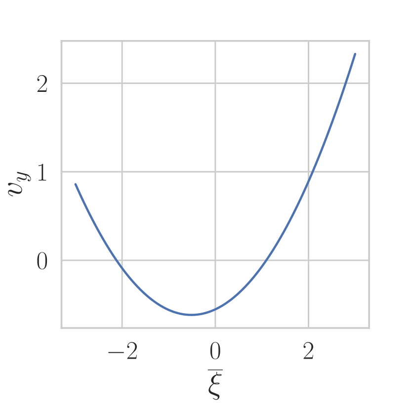
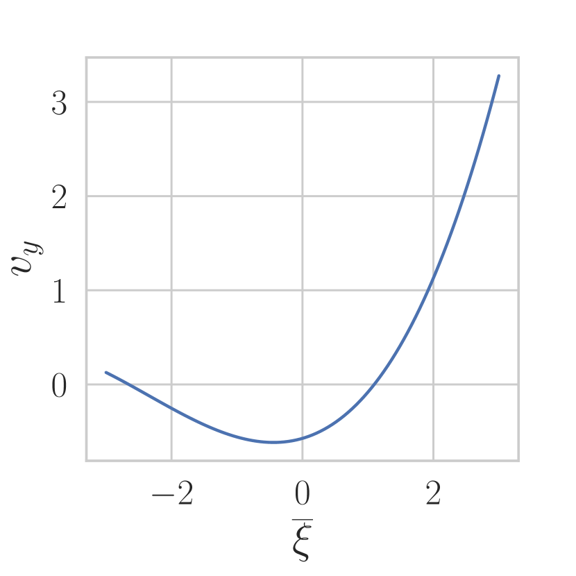
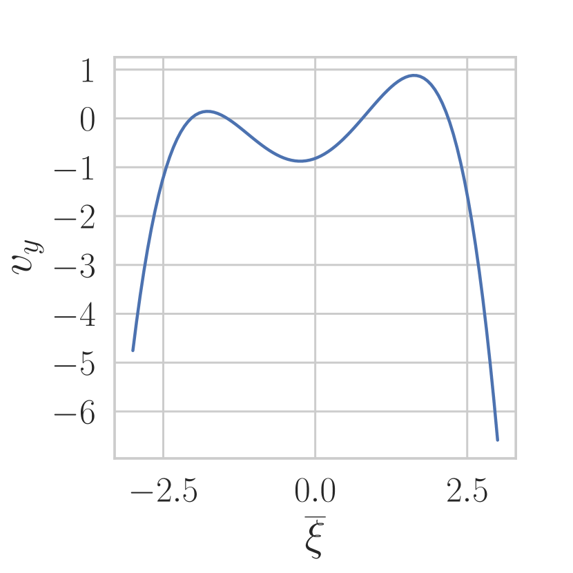
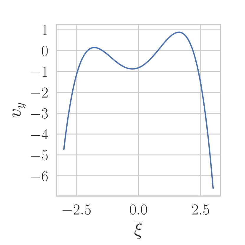
Furthermore, showing the shapes of the polynomials sequentially in Figure 10, up to degree $3$ there is no evidence of bifurcating behavior. Instead, when reaching degree four, three local extrema can be seen in the sampling area. The values of the polynomial in Figure 10(c) corresponding to low-gradient points are particularly interesting, since they correspond to the values reached by the three solution branches at a viscosity value of $0.9$ (see Figure 4).

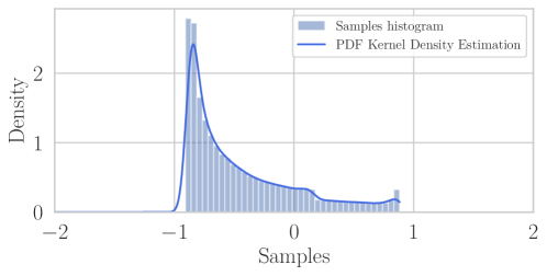
In particular, this insight is supported by Figure 11, where the PDF of the velocity solution of the PC surrogate model with degree $4$ is reconstructed. Indeed, three peaks can be observed at the three local extrema of the polynomial, around the values $\{-1,0,1\}$, respectively. As anticipated before, samples of the velocity variable are obtained by repeatedly applying the polynomial to samples from a normal Gaussian variable $\overline{\xi}$. This is indeed the reason for the higher peak at $-1$ in the density plot since the abscissa of the corresponding local minimum of the polynomial is close to zero and thus more frequent in the sample.

Figure 11. Kernel Density Estimation of the velocity PDF at the domain point of maximum variance.

In addition, it should be noted that the behavior of polynomials keep the same shape for degree five (see Figure 10(d)), suggesting that the velocity probability distribution at that point is completely described by these three local extrema.

6.2. Deterministic bifurcation diagram inference

In this section, we want to study how the previous analysis extends to different parameter values, thus going in the direction of zero knowledge regarding the bifurcation. Thus, the goal is to look for the general behavior of PC polynomials, and their ability to provide information regarding the topology of the deterministic bifurcation diagram seen in the stochastic perturbation context.

First, we are interested in checking the behavior of the variance of the velocity in the uniqueness regime. The results of the SSFEM calculations are shown in Figure 12. When the uniqueness of the solution is ensured, the variance is significantly lower (about four orders of magnitude) than the one observed in the non-uniqueness region (see Figure 9).

(a) Viscosity $\mu\sim\mathcal{N}(1.1,0.001)$ and maximum PC degree of $4$.

(b) Viscosity $\mu\sim\mathcal{N}(1.3,0.001)$ and maximum PC degree of $4$.

Figure 12. Variance of the vertical component of the velocity field solution in the uniqueness regime.

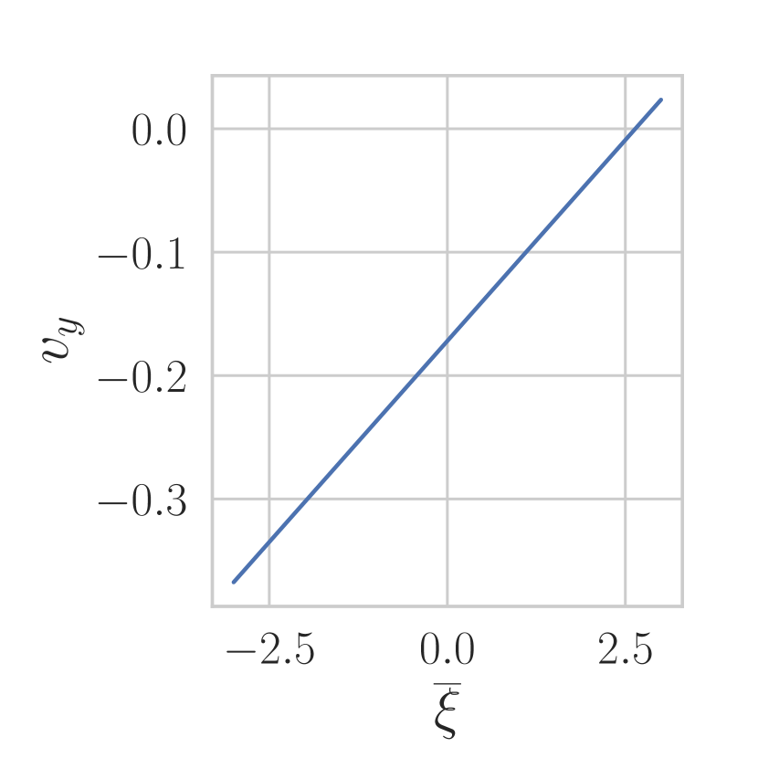
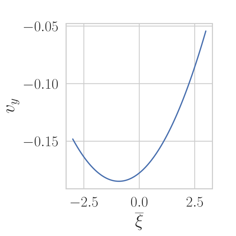
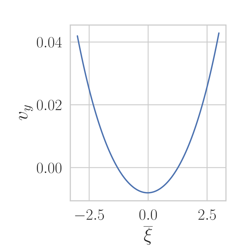
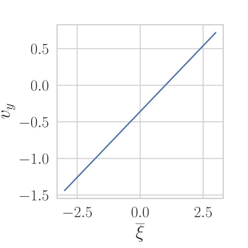
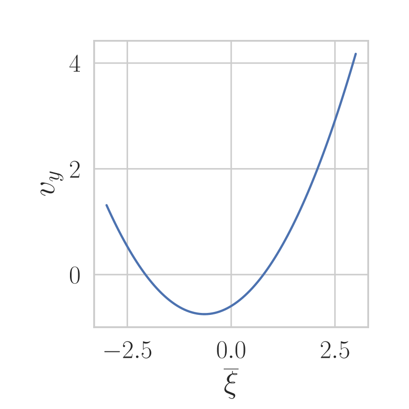
We remark that, by investigating the polynomials corresponding to parameter values for which the solution is unique, their shapes consistently change but still providing the same information regarding the connection between local maxima and number of branches. In fact, taking the point of maximum variance in the cases $\mu\sim\mathcal{N}(1.1,0.001)$ and $\mu\sim\mathcal{N}(1.3,0.001)$, in Figures 13 and 14, even increasing the polynomial degree, only one peak is evident in the sampling zone, contrarily to what happened in the bifurcating regime depicted in Figure 9.

Precisely, in Figure 12(b) the point of maximum variance is different from the previous one, while in the case of Figure 12(a) it remains the same, although the absolute value of variance decreases significantly. However, in both cases of Figure 12 the shapes of the polynomials are similar: multiple local extremes do not appear when the solution is unique, providing a consistent result with the interpretation given in the previous section.

(a) degree $=1$

(b) degree $=2$

(c) degree $=3$

(d) degree $=4$

Figure 13. Evolution of the polynomials in the point of maximum variance in case of $\mu\sim\mathcal{N}(1.1,0.001)$.

(a) degree $=1$

(b) degree $=2$

(c) degree $=3$

(d) degree $=4$

Figure 14. Evolution of the polynomials in the point of maximum variance in case of $\mu\sim\mathcal{N}(1.3,0.001)$.

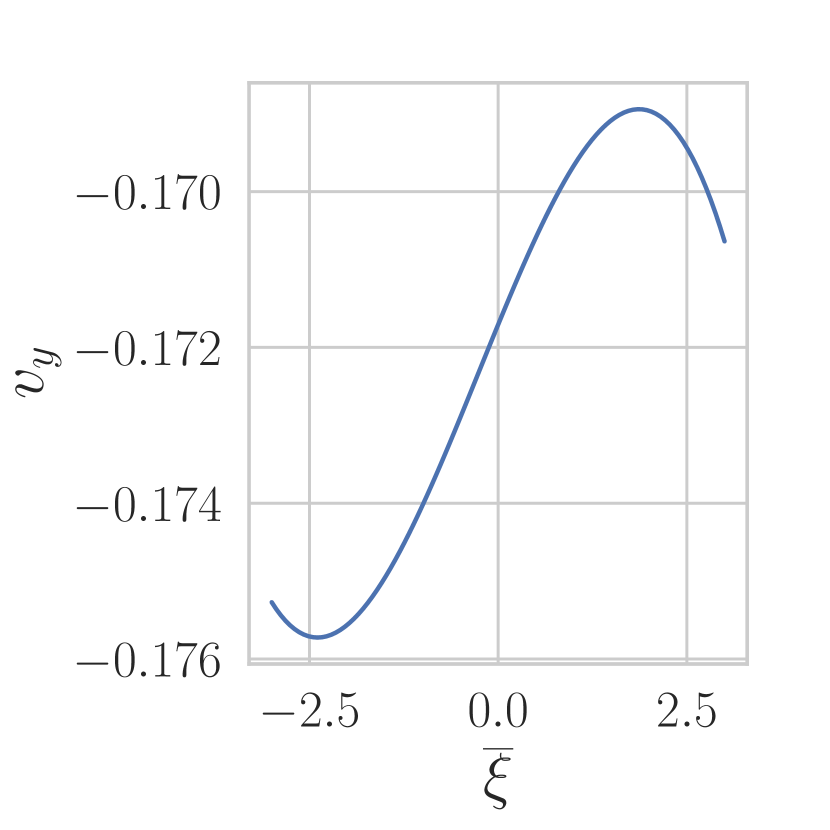
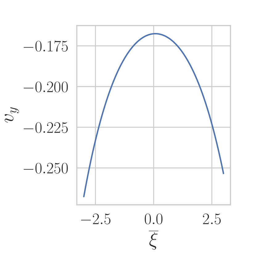
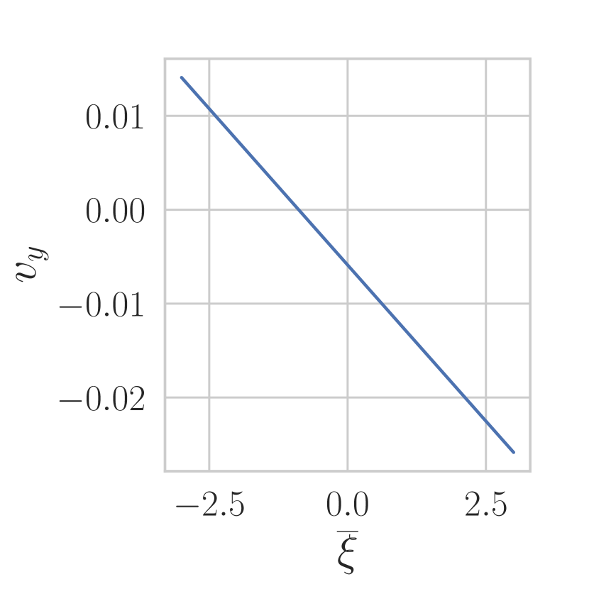
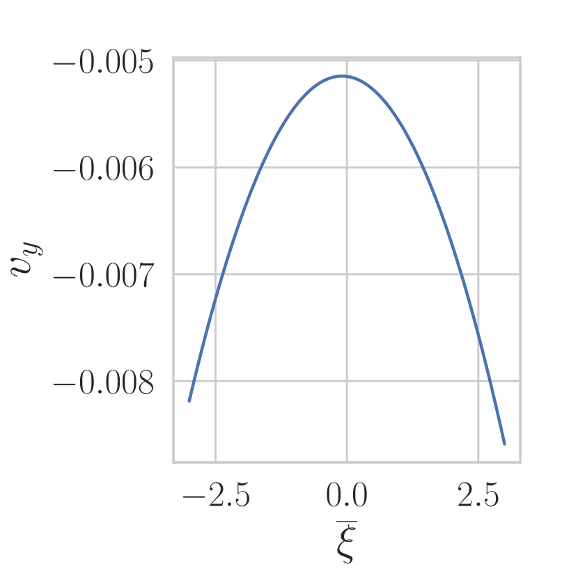
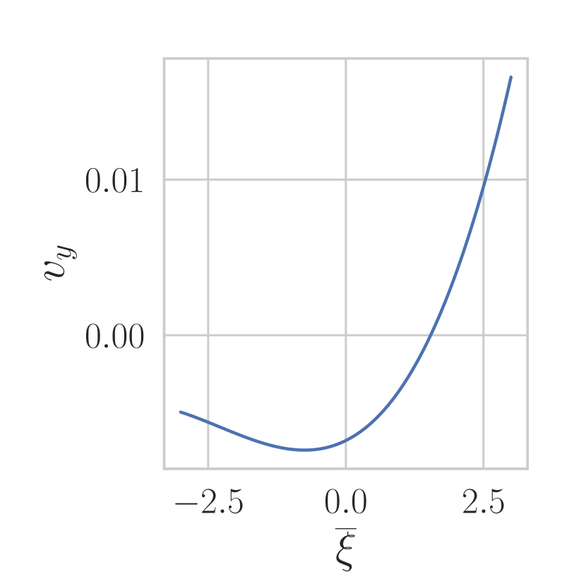
Towards a complete investigation of the bifurcation diagram, we are interested in the possibility of reconstructing the branches for any value of viscosity, without relying on any prior information. To this end, we show the same simulation for viscosity values below the critical bifurcation point $\mu^{*}$. In particular, we report here the results of the SSFEM calculations for $\mu\sim\mathcal{N}(0.85,0.001)$ and $\mu\sim\mathcal{N}(0.8,0.001)$ in Figure 15.

As a first consideration, the magnitude of the variance increases significantly from Figure 10(c)) with viscosity value $0.9$, to Figure 15(b) with value $0.8$. Indeed, this is consistent with the deterministic bifurcation diagram, as the branches become increasingly separated as the viscosity parameter decreases.

(a) Viscosity $\mu\sim\mathcal{N}(0.85,0.001)$ and maximum PC degree of $4$.

(b) Viscosity $\mu\sim\mathcal{N}(0.8,0.001)$ and maximum PC degree of $4$.

Figure 15. Variance of the vertical component of the velocity field solution of Equations (23) in case of non-uniqueness of the velocity solution.

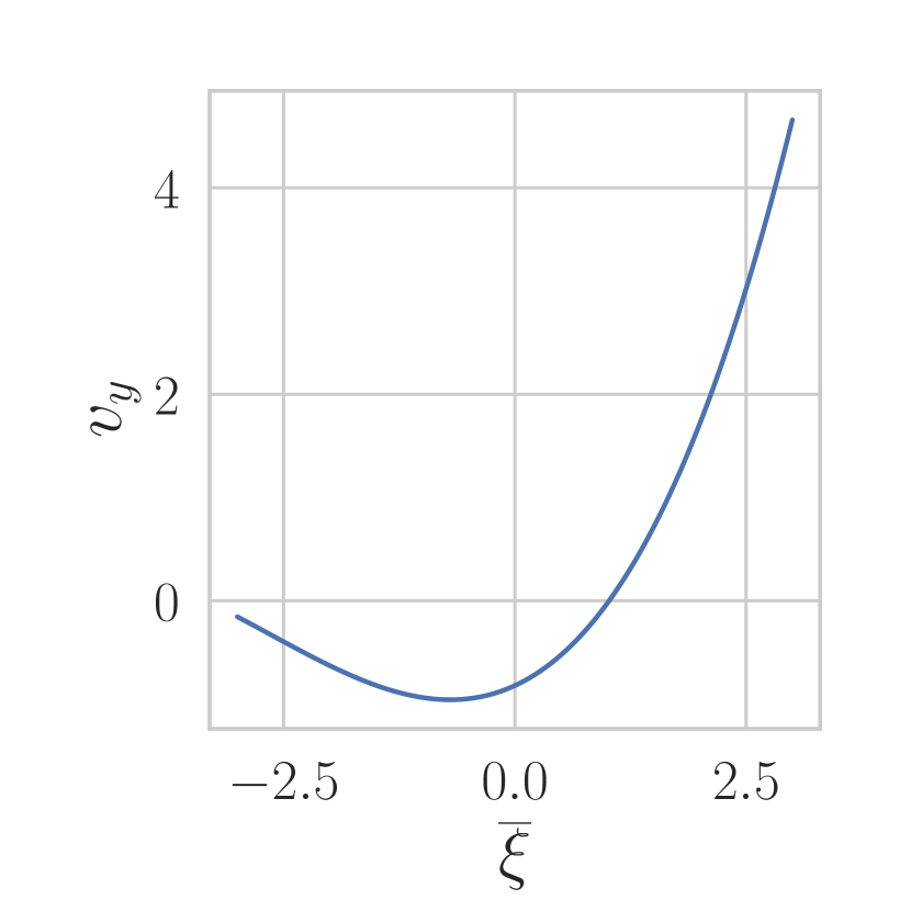
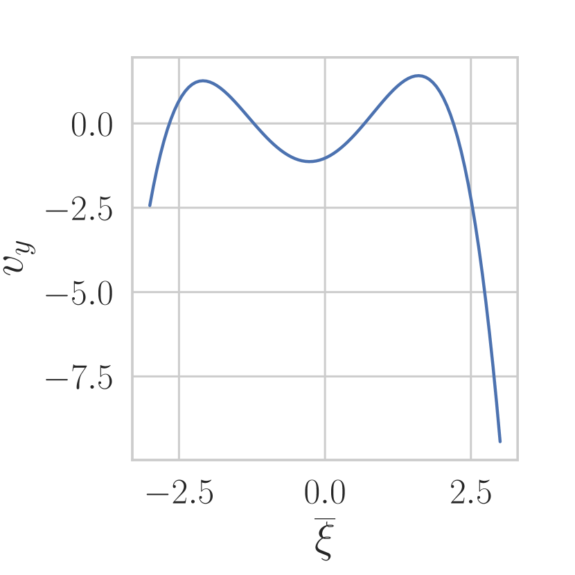
Similar to the analysis performed in 6.1 section, expansion polynomials can be retrieved and sampled according to the distribution of their variables. For polynomials of sufficiently high degree, the samples are concentrated around their local extrema, as it can be seen in Figures 16 and 17, respectively.

(a) degree $=1$

(b) degree $=2$

(c) degree $=3$

(d) degree $=4$

Figure 16. Evolution of the polynomials in the point of maximum variance in case of $\mu\sim\mathcal{N}(0.85,0.001)$.

(a) degree $=1$

(b) degree $=2$

(c) degree $=3$

(d) degree $=4$

Figure 17. Evolution of the polynomials in the point of maximum variance in case of $\mu\sim\mathcal{N}(0.8,0.001)$.

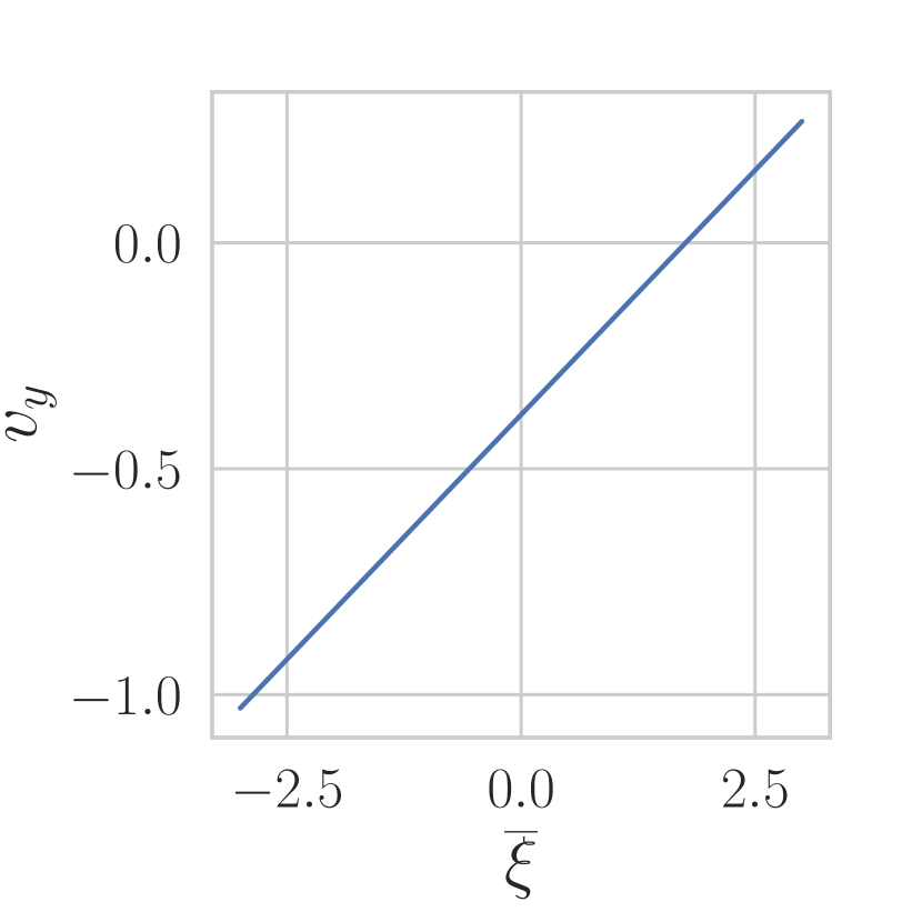
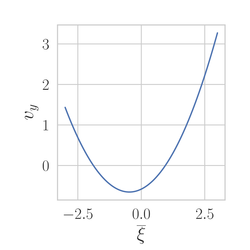
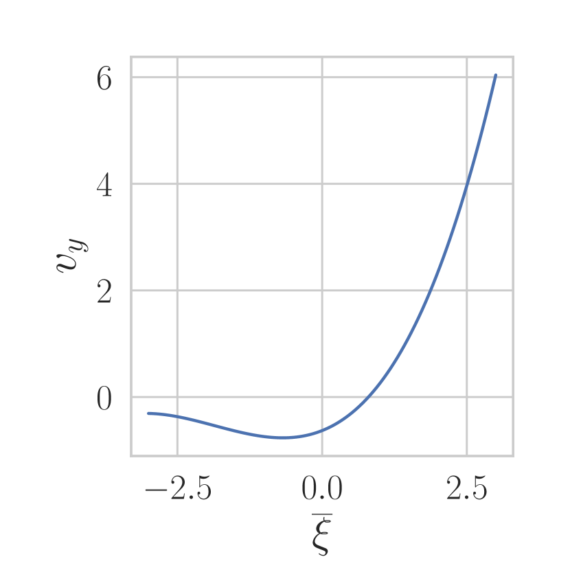
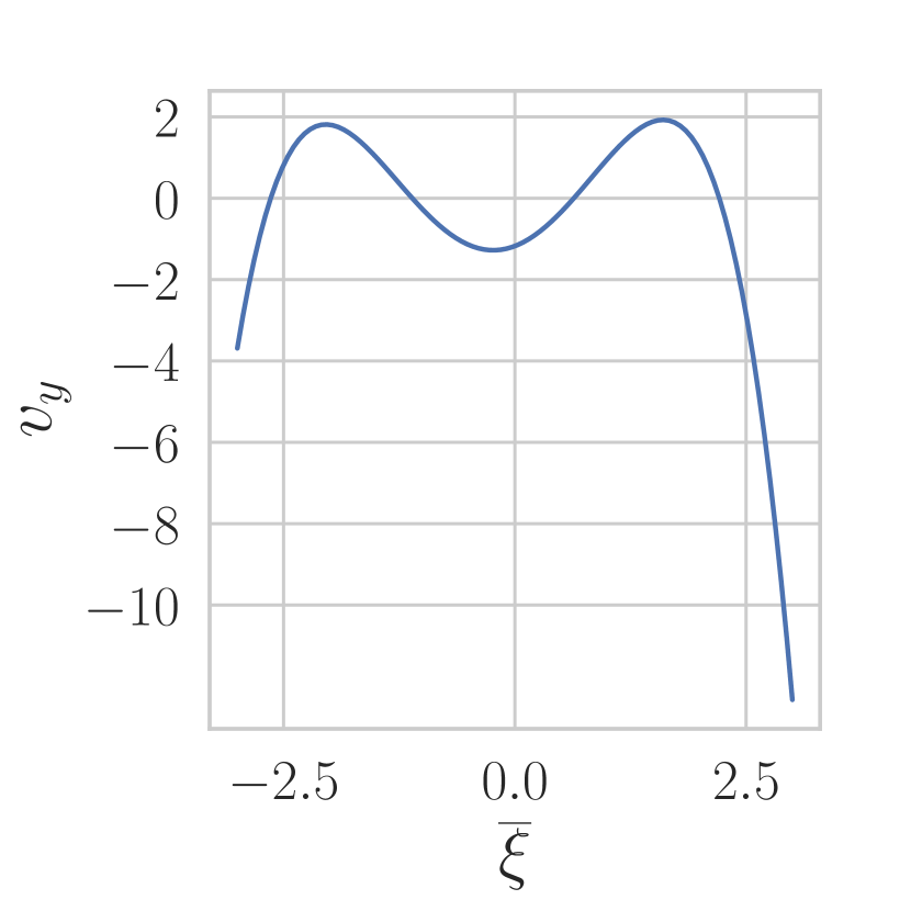
We remark that, in the cases where the branches of the solution progressively separate, the computation of the PC coefficients is typically more expensive initializing the nonlinear solver with a zero guess. In fact, following the interpretation given to the polynomials, higher coefficients must be achieved to fully exploit the capability of the surrogates.

However, by looking at Figures 16 and 17 where $\mu$ is centered in $0.85$ and $0.8$, respectively, three peaks for polynomials of degree 4 are visible in the sampling zone. Moreover, their values increase in absolute value, from a maximum of about $1.5$ in Figure 16(d) to value $2$ in Figure 17(d), while in the case of viscosity centered at $\mu=0.9$, the maximum had value close to $1$. On the other hand, for these new values, given the convergence difficulties highlighted before, the symmetry between positive and negative values of the local extrema is not exactly recovered, and the unstable branch of solutions is more difficult to retrieve.

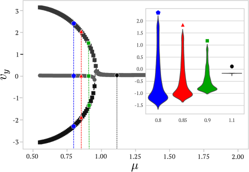
From the exploration of a wider viscosity range, we can have some confirmation regarding the argument raised in the previous section, connecting the number of coexisting solution branches with the number of local extrema for the PC surrogates in the sampling zone. Moreover, we can exploit the results obtained in the previous stochastic analysis to obtain a probabilistic version of the bifurcation diagram, shown in Figure 18. From this plot we recognize the general tendency of these extrema to follow the branches of the deterministic bifurcation diagram. In Figure 18, we report the deterministic bifurcation diagram, highlighting with different markers the admissible solutions for different viscosity parameters. By displaying the density plot related to the solution of the stochastic PDE for the viscosity perturbed around these values, we observe that the branches of the solution are exactly recovered in the case of $\mu=0.9$, and that for $\mu=1.1$ the density of the solution is concentrated on a single value, corresponding to the unique solution. Even when considering viscosity values in the “strong” bifurcation regime, namely $\mu=0.85$ and $\mu=0.8$, the evolution of the branches is followed, although the lower branch is not perfectly recovered in its symmetry due to convergence difficulties.

Figure 18. Reconstruction of the solution branches through the probabilistic solution obtained via the SSFEM computations for different viscosity values.

7. Conclusions and Perspectives

In this work, we proposed a numerical stochastic-perturbation approach to deterministic bifurcation problems. We developed an intrusive pipeline based on the Spectral Stochastic Finite Element Method approach to retrieve the expansion coefficients, and we found that the Polynomial Chaos expansion of the solution successfully encode accurate information about the bifurcation diagram.

For what concerns the PC surrogate model of a stochastic bifurcating PDE, we showed the strict relation between the branches of coexisting solutions, and the local extrema of the corresponding PC functions. Indeed, the number of local extrema in the sampling region corresponds to the number of the solution branches for the specific parameter value at which the distribution is centered. Moreover, the height of such local extrema match the values of the branches, leading to the formation of clusters of points around them when the solution is sampled.

The intrusive approach helps in overcoming the issues arising in the bifurcating setting, as it does not require any prior knowledge about the solution branches. Indeed, in the non–intrusive case, computing samples of the parametric solution in the non–uniqueness regime, require the need for additional information about the bifurcating behavior in the sampling strategy. This precaution allows the numerical solver to converge to different branches, and thus to provide a complete overview of the solution manifold via a meaningful and representative ensemble of admissible configurations. As a result, SSFEM offers a significant advantage by being independent of problem-specific initialization, while still providing a precise representation of the complete solution manifold.

On the other hand, from a strictly computational point of view, the SSFEM intrusive approach may be expensive due to the dimension of the system to be solved for high polynomial degrees, as discussed in Section 6. This poses new computational challenges, which can be mitigated through ad-hoc convergence strategies and preconditioning methods, as shown in previous works,including those addressing the Navier–Stokes equations [47, 31]. Therefore, important improvements could be achieved, enabling faster computation of higher order coefficients and allowing for the analysis of more complex behaviours, such as the case of higher Reynolds numbers in the Navier–Stokes setting, where successive bifurcations emerge.

Additional investigations could focus on the source of stochasticity in the system. For instance, the study of random initial and/or boundary conditions may play an important role in the evolution of the system for time-dependent problems. This could be used to infer a probabilistic overview of the system’s behaviour, understanding statistical properties of the branches.

Finally, given the numerous reliable surrogate models for the probability distribution of the solution, it is worth exploring a Bayesian approach to the bifurcation problem, following the framework proposed in [24]. Indeed, incorporating real data into the analysis could be particularly important to discover the complex behaviour of a real–world parametric system. This could bring model’s improvements in its reality reproduction capability, which is of crucial importance in many engineering tasks.

References

- [1] E. L. Allgower and K. Georg. Introduction to numerical continuation methods. SIAM, 2003.
- [2] A. Ambrosetti and G. Prodi. A Primer of Nonlinear Analysis. Cambridge Studies in Advanced Mathematics. Cambridge University Press, 1995.
- [3] N. Arcozzi, M. Campanino, and G. Giambartolomei. The karhunen-loeve theorem.
- [4] L. Arnold. Stochastic systems: Qualitative theory and lyapunov exponents. In W. Horsthemke and D. K. Kondepudi, editors, Fluctuations and Sensitivity in Nonequilibrium Systems, pages 11–18, Berlin, Heidelberg, 1984. Springer Berlin Heidelberg.
- [5] L. Arnold. Random dynamical systems. Springer, 2010.
- [6] L. Arnold and P. Boxler. Stochastic bifurcation: instructive examples in dimension one, pages 241–255. Birkhäuser Boston, Boston, MA, 1992.
- [7] I. Babuška, F. Nobile, and R. Tempone. A stochastic collocation method for elliptic partial differential equations with random input data. SIAM Journal on Numerical Analysis, 45(3):1005–1034, 2007.
- [8] P. Benner, A. Cohen, M. Ohlberger, and K. Willcox. Model Reduction and Approximation: Theory and Algorithms. SIAM, Society for Industrial and Applied Mathematics, 2017.
- [9] A. Blumenthal, M. Engel, and A. Neamtu. On the pitchfork bifurcation for the Chafee-Infante equation with additive noise. Probability Theory and Related Fields, August 2021.
- [10] N. Boullé, P. E. Farrell, and A. Paganini. Control of Bifurcation Structures using Shape Optimization. SIAM Journal on Scientific Computing, 44(1):A57–A76, 2022.
- [11] J. R. Bravo, G. Stabile, M. Hess, J. A. Hernandez, R. Rossi, and G. Rozza. Geometrically Parametrised Reduced Order Models for the Study of Hysteresis of the Coanda Effect in Finite-elements-based Incompressible Fluid Dynamics, 2023.
- [12] S. L. Brunton, J. L. Proctor, and J. N. Kutz. Discovering governing equations from data by sparse identification of nonlinear dynamical systems. Proceedings of the National Academy of Sciences, 113(15):3932–3937, 2016.
- [13] G. Caloz and J. Rappaz. Numerical analysis for nonlinear and bifurcation problems. In Handbook of Numerical Analysis, volume 5 of Techniques of Scientific Computing (Part 2), pages 487–637. Elsevier, 1997.
- [14] R. H. Cameron and W. T. Martin. The orthogonal development of non-linear functionals in series of fourier-hermite functionals. Annals of Mathematics, 48:385, 1947.
- [15] G. Carere, M. Strazzullo, F. Ballarin, G. Rozza, and R. Stevenson. A weighted POD-reduction approach for parametrized PDE-constrained optimal control problems with random inputs and applications to environmental sciences. Computers & Mathematics with Applications, 102:261–276, 2021.
- [16] W. Cherdron, F. Durst, and J. H. Whitelaw. Asymmetric flows and instabilities in symmetric ducts with sudden expansions. Journal of Fluid Mechanics, 84(1):13–31, 1978.
- [17] K. A. Cliffe, A. Spence, and S. J. Tavener. The numerical analysis of bifurcation problems with application to fluid mechanics. Acta Numerica, 9:39–131, January 2000.
- [18] D. Coscia, N. Demo, and G. Rozza. Generative adversarial reduced order modelling. Scientific Reports, 14(1):3826, 2024.
- [19] R. Crisovan, D. Torlo, R. Abgrall, and S. Tokareva. Model order reduction for parametrized nonlinear hyperbolic problems as an application to uncertainty quantification. Journal of Computational and Applied Mathematics, 348:466–489, 2019.
- [20] E. J. Doedel, H. B. Keller, and J. P. Kernevez. Numerical analysis and control of bifurcation problems (i): bifurcation in finite dimensions. International Journal of Bifurcation and Chaos, 01(03):493–520, 1991.
- [21] O. G. Ernst, A. Mugler, H.-J. Starkloff, and E. Ullmann. On the convergence of generalized polynomial chaos expansions. ESAIM: Mathematical Modelling and Numerical Analysis, 46(2):317–339, 2012.
- [22] P. E. Farrell, Á. Birkisson, and S. W. Funke. Deflation Techniques for Finding Distinct Solutions of Nonlinear Partial Differential Equations. SIAM Journal on Scientific Computing, 37(4):A2026–A2045, 2015.
- [23] R. G. Ghanem and P. D. Spanos. Stochastic finite elements: A spectral approach. 1990.
- [24] M. Girolami, E. Febrianto, G. Yin, and F. Cirak. The statistical finite element method (statfem) for coherent synthesis of observation data and model predictions. Computer Methods in Applied Mechanics and Engineering, 375:113533, March 2021.
- [25] J. S. Hesthaven, G. Rozza, and B. Stamm. Certified Reduced Basis Methods for Parametrized Partial Differential Equations. SpringerBriefs in Mathematics. Springer International Publishing, 2015.
- [26] S. Huang, S. Quek, and K. Phoon. Convergence study of the truncated karhunen–loeve expansion for simulation of stochastic processes. International journal for numerical methods in engineering, 52(9):1029–1043, 2001.
- [27] S. Janson. Gaussian Hilbert Spaces. Cambridge Tracts in Mathematics. Cambridge University Press, 1997.
- [28] K. Karhunen. Zur spektraltheorie stochastischer prozesse. 1946.
- [29] M. Khamlich, F. Pichi, and G. Rozza. Model order reduction for bifurcating phenomena in fluid-structure interaction problems. International Journal for Numerical Methods in Fluids, 94(10):1611–1640, 2022.
- [30] M. Khamlich, F. Pichi, and G. Rozza. Model order reduction for bifurcating phenomena in fluid‐structure interaction problems. International Journal for Numerical Methods in Fluids, 94(10):1611–1640, June 2022.
- [31] K. Lee, H. C. Elman, and B. Sousedík. A low-rank solver for the navier–stokes equations with uncertain viscosity. SIAM/ASA Journal on Uncertainty Quantification, 7(4):1275–1300, 2019.
- [32] P. Lévy. Processus stochastiques et mouvement brownien. Suivi d’une note de M. Loève. Paris: Gauthier-Villars, Éditeur 365 p. (1948)., 1948.
- [33] M. Liu. Stability and dynamical bifurcation of a stochastic regime-switching predator–prey model. Journal of Mathematical Analysis and Applications, 535(1):128096, 2024.
- [34] E. Mirzakhalili and B. I. Epureanu. Probabilistic analysis of bifurcations in stochastic nonlinear dynamical systems. Journal of Computational and Nonlinear Dynamics, 14(8), June 2019.
- [35] F. Pichi. Reduced order models for parametric bifurcation problems in nonlinear PDEs. PhD thesis, Scuola Internazionale Superiore di Studi Avanzati, Trieste, 2020.
- [36] F. Pichi, F. Ballarin, G. Rozza, and J. S. Hesthaven. An artificial neural network approach to bifurcating phenomena in computational fluid dynamics. Computers & Fluids, 254:105813, 2023.
- [37] F. Pichi, B. Moya, and J. S. Hesthaven. A graph convolutional autoencoder approach to model order reduction for parametrized PDEs. Journal of Computational Physics, 501:112762, 2024.
- [38] F. Pichi, M. Strazzullo, F. Ballarin, and G. Rozza. Driving bifurcating parametrized nonlinear PDEs by optimal control strategies: Application to Navier–Stokes equations with model order reduction. ESAIM: Mathematical Modelling and Numerical Analysis, 56(4):1361–1400, 2022.
- [39] M. Pintore, F. Pichi, M. Hess, G. Rozza, and C. Canuto. Efficient computation of bifurcation diagrams with a deflated approach to reduced basis spectral element method. Advances in Computational Mathematics, 47(1), December 2020.
- [40] G. Pitton and G. Rozza. On the application of reduced basis methods to bifurcation problems in incompressible fluid dynamics. Journal of Scientific Computing, 73(1):157–177, Apr 2017.
- [41] A. Quaini, R. Glowinski, and S. Čanić. Symmetry breaking and preliminary results about a Hopf bifurcation for incompressible viscous flow in an expansion channel. International Journal of Computational Fluid Dynamics, 30(1):7–19, 2016.
- [42] A. Quarteroni. Numerical Models for Differential Problems. MS&A Series Vol. 16. Springer International Publishing, 2017.
- [43] R. Y. Rubinstein and D. P. Kroese. Simulation and the Monte Carlo Method. Wiley, November 2016.
- [44] R. Seydel. Practical Bifurcation and Stability Analysis. Interdisciplinary Applied Mathematics. Springer New York, 2009.
- [45] R. C. Smith. Uncertainty Quantification: Theory, Implementation, and Applications. Society for Industrial and Applied Mathematics, January 2013.
- [46] I. J. Sobey and P. G. Drazin. Bifurcations of two-dimensional channel flows. Journal of Fluid Mechanics, 171:263–287, 1986.
- [47] B. Sousedík and H. C. Elman. Stochastic galerkin methods for the steady-state navier–stokes equations. Journal of Computational Physics, 316:435–452, 2016.
- [48] N. Sri Namachchivaya. Stochastic bifurcation. Applied Mathematics and Computation, 38(2):101–159, 1990.
- [49] G. Stefanou. The stochastic finite element method: Past, present and future. Computer Methods in Applied Mechanics and Engineering, 198(9–12):1031–1051, February 2009.
- [50] B. Sudret. Global sensitivity analysis using polynomial chaos expansions. Reliability Engineering & System Safety, 93(7):964–979, July 2008.
- [51] T. J. Sullivan. Introduction to uncertainty quantification, volume 63. Springer, 2015.
- [52] N. Tonicello, A. Lario, G. Rozza, and G. Mengaldo. Non-intrusive reduced order models for the accurate prediction of bifurcating phenomena in compressible fluid dynamics, 2022.
- [53] D. J. Tritton. Physical fluid dynamics. Springer Science & Business Media, 2012.
- [54] D. Venturi, X. Wan, and G. E. Karniadakis. Stochastic bifurcation analysis of rayleigh–bénard convection. Journal of Fluid Mechanics, 650:391–413, 2010.
- [55] N. Wiener. The homogeneous chaos. American Journal of Mathematics, 60(4):897–936, 1938.
- [56] D. Xiu. Numerical methods for stochastic computations: a spectral method approach. Princeton university press, 2010.
- [57] D. Xiu and G. E. Karniadakis. The wiener–askey polynomial chaos for stochastic differential equations. SIAM Journal on Scientific Computing, 24(2):619–644, 2002.
- [58] D. Xiu and G. E. Karniadakis. Modeling uncertainty in flow simulations via generalized polynomial chaos. Journal of Computational Physics, 187(1):137–167, May 2003.
- [59] A. Zarghami, M. J. Maghrebi, S. Ubertini, and S. Succi. Modeling of bifurcation phenomena in suddenly expanded flows with a new finite volume lattice boltzmann method. International Journal of Modern Physics C, 22(09):977–1003, September 2011.