Finite element schemes with tangential motion for fourth order geometric curve evolutions in arbitrary codimension

Abstract

We introduce novel finite element schemes for curve diffusion and elastic flow in arbitrary codimension. The schemes are based on a variational form of a system that includes a specifically chosen tangential motion. We derive optimal $L^{2}$– and $H^{1}$–error bounds for continuous-in-time semidiscrete finite element approximations that use piecewise linear elements. In addition, we consider fully discrete schemes and, in the case of curve diffusion, prove unconditional stability for it. Finally, we present several numerical simulations, including some convergence experiments that confirm the derived error bounds. The presented simulations suggest that the tangential motion leads to equidistribution in practice.

Key words. curve diffusion; elastic flow; curve straightening flow; finite elements; tangential motion; error analysis; arbitrary codimension

AMS subject classifications. 65M60, 65M12, 65M15, 35K55

1 Introduction

Curves endowed with a geometric energy, and gradient flows related to these energies, are of interest in differential geometry, materials science, continuum mechanics, biological applications, microelectronics and computer vision, [34, 32, 29, 39, 20]. Two of the most frequently studied energies are the length functional

$$L(\Gamma)=\int_{\Gamma}1\;{\rm d}s$$ (1.1)

and the elastic energy

$$E(\Gamma)=\tfrac{1}{2}\int_{\Gamma}|\varkappa|^{2}\;{\rm d}s+\lambda L(\Gamma).$$ (1.2)

Observe that (1.2) combines a bending energy involving the modulus of the curvature vector $\varkappa$ of the curve $\Gamma$ with a length contribution that penalizes growth if $\lambda>0$. In this paper we consider the case of closed curves evolving in ${\mathbb{R}}^{d}$ with $d\geq 2$ arbitrary. The most natural gradient flows for (1.1) and (1.2) are their respective $L^{2}$–gradient flows, giving rise to curve shortening flow, [26, 30], and elastic flow (also called curve straightening flow), [40, 35, 22]. In the case of (1.1) the $H^{-1}$–gradient flow is also of interest, and leads to curve diffusion, [38, 24, 25, 27, 28, 22, 8]. In the planar case, $d=2$, this flow is often also called surface diffusion for curves and has the important property of conserving the area enclosed by the curve. In fact, surface diffusion was proposed in [34] as an evolution law for a free surface enclosing a solid phase, which changes its shape due to the diffusion of atoms along the surface. Later a derivation in the context of rational thermodynamics was given in [13].
In this paper, we investigate the numerical approximation of curve diffusion and elastic flow. It turns out that both of these fourth order geometric evolution equations are closely related, and so our numerical analysis can be applied to both cases with only minor modifications. From now on, and throughout this paper, we consider a parametric description of the family of evolving curves $(\Gamma(t))_{t\in[0,T]}$, $T>0$. In particular, we assume that $\Gamma(t)=x(I,t)$, where $I={{\mathbb{R}}}/{\mathbb{Z}}$ is the periodic unit interval and $x:I\times[0,T]\to{\mathbb{R}}^{d}$. On letting $\cdot_{s}$ denote differentiation with respect to arclength, the unit tangent along the curve is $\tau=x_{s}$. Then $x$ parameterizes a family of curves moving by curve diffusion if it satisfies the partial differential equation

$$Px_{t}=-\nabla_{\!s}^{2}\varkappa,$$ (1.3)

where $P=I\!d-\tau\otimes\tau$ and $\nabla_{\!s}\phi=P\phi_{s}$ for a vector field $\phi$. Similarly, elastic flow is described by solutions to

$$Px_{t}=-\nabla_{\!s}^{2}\varkappa-\tfrac{1}{2}|\varkappa|^{2}\varkappa+\lambda\varkappa.$$ (1.4)

Observe that the tangential velocity, $x_{t}\cdot\tau$, is not prescribed in (1.3) and (1.4), which is a natural consequence of the fact that reparameterizations of the evolving family of curves does not affect the geometric evolution.
It is the aim of this paper to introduce a suitable tangential motion in (1.3) and (1.4) in such a way that the obtained system of partial differential equations

• is strictly parabolic,

• asymptotically exhibits solutions that are nearly arclength parameterizations,

• admits a weak formulation that is amenable to discretization by finite elements with a corresponding error analysis.

Our approach will be first developed for the curve diffusion flow. The main idea is to require the tangential motion to be such that $x$ not only satisfies (1.3), but in addition reduces its Dirichlet energy $\int_{I}|x_{\rho}|^{2}\;{\rm d}\rho$ in time, thus driving the parameterization towards one that is proportional to arclength. This idea can be viewed as a natural extension of similar approaches for the curve shortening flow ([15, 23]) to the fourth order problem. Intuitively it is clear that on the discrete level this will yield nice distributions of mesh points, since large deviations in the length element $|x_{\rho}|$ are penalized. In fact, in practice we do observe asymptotically equidistributed discretizations for the schemes introduced and analysed in this paper.
Let us briefly review the existing literature on numerical approximations of parametric formulations for curve diffusion and elastic flow, with a particular emphasis on the available error analysis. Various numerical schemes for curve diffusion have been proposed in [22, 3, 33, 6, 8, 9, 5, 31, 4]. To the best of our knowledge, no error bounds for such schemes have been proved so far. But we mention the results in [2, 17] for the error analysis of surface diffusion, for the case of hypersurfaces evolving in ${\mathbb{R}}^{3}$, in the context of graph formulations. With regards to elastic flow, numerical methods have been proposed in [22, 6, 7, 16, 8, 10, 12, 36]. In [16] error estimates are shown, while [12] contains a partial convergence result for a scheme that approximates elastic flow of inextensible curves. Here we recall that the numerical methods in [22, 16] discretize a purely normal flow, which can lead to very nonuniform meshes and coalescence of vertices in practice. The BGN-schemes from the series of papers [6, 7, 8, 10, 9], on the other hand, enjoy nearly uniform distributions of mesh points in practice, see also [5, 31] for related contributions and [33, 21] for alternative approaches involving tangential motion. But for now there is no error analysis for these schemes. A first step to combine error analysis and good mesh properties for fourth order flows was recently achieved in [36]. There a gradient flow for an energy functional like (1.2), but with the length of the curve replaced by the Dirichlet energy $\int_{I}|x_{\rho}|^{2}\;{\rm d}\rho$, was introduced and analysed. Since the Dirichlet energy is not invariant with respect to reparameterization, the resulting flow is no longer geometric. Nevertheless, this modified flow has the same stationary points as elastic flow. For more details on discretization methods for geometric partial differential equations we refer to the two review articles [18, 11].
We end this section with a few comments about notation. Throughout, $C$ denotes a generic positive constant independent of the mesh parameter $h$. At times $\varepsilon$ will play the role of a (small) positive parameter, with $C_{\varepsilon}>0$ depending on $\varepsilon$, but independent of $h$.

2 Mathematical formulation

Consider a family $(\Gamma(t))_{t\in[0,T]}$ of evolving curves that are given by $\Gamma(t)=x(I,t)$, where $x:I\times[0,T]\to{\mathbb{R}}^{d}$ satisfies $|x_{\rho}|>0$ in $I\times[0,T]$. Then the unit tangent on $\Gamma(t)$, the curvature vector of $\Gamma(t)$ and the orthogonal projection onto the normal space of $\Gamma(t)$ are given by the following identities in $I$, see e.g. [11]:

$$\tau=x_{s}=\frac{x_{\rho}}{|x_{\rho}|},\quad\varkappa=\frac{\tau_{\rho}}{|x_{\rho}|}=\frac{1}{|x_{\rho}|}\bigl{(}\frac{x_{\rho}}{|x_{\rho}|}\bigr{)}_{\rho},\quad P=I\!d-\tau\otimes\tau.$$

With a view towards introducing variational discretizing methods for curve diffusion, (1.3), and elastic flow, (1.4), we follow the common approach of rewriting these fourth order problems in terms of two second order problems for the position vector $x$ and a further variable $y$. Rather than making the frequent choice $y=\varkappa$, in this paper we take

$$y=\frac{x_{\rho\rho}}{|x_{\rho}|^{2}},$$ (2.1)

so that

$$\varkappa=\frac{x_{\rho\rho}}{|x_{\rho}|^{2}}-\frac{x_{\rho\rho}\cdot x_{\rho}}{|x_{\rho}|^{3}}\frac{x_{\rho}}{|x_{\rho}|}=Py.$$

The idea to use (2.1) as a second variable extends the approach from [15], where the formulation $x_{t}=\frac{x_{\rho\rho}}{|x_{\rho}|^{2}}$ was used for curve shortening flow, to the fourth order flows considered in this paper.
Observing that $P_{s}=-\tau_{s}\otimes\tau-\tau\otimes\tau_{s}=-Py\otimes\tau-\tau\otimes Py$, we calculate

$$\nabla_{\!s}\varkappa=(Py)_{s}-\bigl{(}(Py)_{s}\cdot\tau\bigr{)}\tau=P\bigl{(}Py_{s}+P_{s}y\bigr{)}=Py_{s}-(\tau\cdot y)Py,$$

and hence

$$\nabla_{\!s}^{2}\varkappa =P\bigl{(}Py_{ss}+P_{s}y_{s}\bigr{)}-P\bigl{(}(\tau_{s}\cdot y)Py+(\tau\cdot y_{s})Py+(\tau\cdot y)P_{s}y+(\tau\cdot y)Py_{s}\bigr{)}$$

$$=Py_{ss}-2(\tau\cdot y_{s})Py-|Py|^{2}Py+(\tau\cdot y)^{2}Py-(\tau\cdot y)Py_{s}$$

$$=Py_{ss}-2(\tau\cdot y_{s})Py-|y|^{2}Py+2(\tau\cdot y)^{2}Py-(\tau\cdot y)Py_{s}.$$ (2.2)

Moreover, we have on noting (2.1) that

$$y_{s}=\frac{y_{\rho}}{|x_{\rho}|},\quad y_{ss}=\frac{1}{|x_{\rho}|}\left(\frac{y_{\rho}}{|x_{\rho}|}\right)_{\rho}=\frac{1}{|x_{\rho}|^{2}}y_{\rho\rho}-(y\cdot\tau)\frac{y_{\rho}}{|x_{\rho}|}.$$ (2.3)

Combining (2) and (2.3) yields that

$$\nabla_{\!s}^{2}\varkappa =P\frac{y_{\rho\rho}}{|x_{\rho}|^{2}}-2(\frac{y_{\rho}}{|x_{\rho}|}\cdot\tau)Py-2(y\cdot\tau)P\frac{y_{\rho}}{|x_{\rho}|}+2(y\cdot\tau)^{2}Py-|y|^{2}Py$$

$$=\frac{1}{|x_{\rho}|^{2}}P\left[y_{\rho\rho}-2(y_{\rho}\cdot x_{\rho})y-2(y\cdot x_{\rho})y_{\rho}+2(y\cdot x_{\rho})^{2}y-|x_{\rho}|^{2}|y|^{2}y\right].$$ (2.4)

2.1 Curve diffusion

Our aim now is to introduce a system in such a way that (1.3) holds, while the tangential part is chosen suitable to give desired properties. Starting from (2) , the most general ansatz would hence be to consider the system

$$x_{t}=\frac{1}{|x_{\rho}|^{2}}\left(-y_{\rho\rho}+2(y_{\rho}\cdot x_{\rho})y+2(y\cdot x_{\rho})y_{\rho}-2(y\cdot x_{\rho})^{2}y+|x_{\rho}|^{2}|y|^{2}y\right)+\alpha\frac{x_{\rho}}{|x_{\rho}|^{2}},$$ (2.5)

whose solutions clearly satisfy (1.3), i.e. $Px_{t}=-\nabla_{\!s}^{2}\varkappa$ and therefore $\frac{\rm d}{{\rm d}t}\int_{I}|x_{\rho}|\;{\rm d}\rho\leq 0$ as a parameterization of the $H^{-1}$–gradient flow of length. Motivated by analogous properties for the DeTurck trick applied to curve shortening flow, see [15], we now attempt to find a coefficient $\alpha$ such that solutions to (2.5) satisfy in addition

$$\frac{\rm d}{{\rm d}t}\int_{I}|x_{\rho}|^{2}\;{\rm d}\rho\leq 0.$$ (2.6)

To this end, we compute with the help of (2.1) and (2.5) that

$$\tfrac{1}{2}\frac{\rm d}{{\rm d}t}\int_{I}|x_{\rho}|^{2}\;{\rm d}\rho =\int_{I}x_{\rho}\cdot x_{\rho,t}\;{\rm d}\rho=-\int_{I}y\cdot x_{t}|x_{\rho}|^{2}\;{\rm d}\rho$$

$$=-\int_{I}|y_{\rho}|^{2}\;{\rm d}\rho-2\int_{I}y_{\rho}\cdot x_{\rho}|y|^{2}\;{\rm d}\rho-2\int_{I}(y\cdot x_{\rho})y_{\rho}\cdot y\;{\rm d}\rho$$

$$\quad+2\int_{I}(y\cdot x_{\rho})^{2}|y|^{2}\;{\rm d}\rho-\int_{I}|x_{\rho}|^{2}|y|^{4}\;{\rm d}\rho-\alpha\int_{I}x_{\rho}\cdot y\;{\rm d}\rho$$

$$=-\int_{I}|y_{\rho}|^{2}+2y_{\rho}\cdot x_{\rho}|y|^{2}+|x_{\rho}|^{2}|y|^{4}\;{\rm d}\rho$$

$$\quad-\int_{I}y\cdot x_{\rho}[2y_{\rho}\cdot y-2y\cdot x_{\rho}|y|^{2}+\alpha]\;{\rm d}\rho$$

$$=-\int_{I}|y_{\rho}+|y|^{2}x_{\rho}|^{2}\;{\rm d}\rho-\int_{I}y\cdot x_{\rho}[2y_{\rho}\cdot y-2y\cdot x_{\rho}|y|^{2}+\alpha]\;{\rm d}\rho.$$

Choosing

$$\alpha=2y\cdot x_{\rho}|y|^{2}-2y_{\rho}\cdot y$$

we find that solutions of the system

$$x_{t} =\frac{1}{|x_{\rho}|^{2}}\left(-y_{\rho\rho}+2(y_{\rho}\cdot x_{\rho})y+2(y\cdot x_{\rho})y_{\rho}-2(y\cdot x_{\rho})^{2}y+|x_{\rho}|^{2}|y|^{2}y\right)$$

$$\quad+\frac{2}{|x_{\rho}|^{2}}\left(y\cdot x_{\rho}|y|^{2}-y\cdot y_{\rho}\right)x_{\rho}$$ (2.7)

satisfy (1.3) and have the desired property (2.6). In particular, solutions to (2.1) satisfy the identity

$$\frac{\rm d}{{\rm d}t}\int_{I}|x_{\rho}|^{2}+\int_{I}|y_{\rho}+|y|^{2}x_{\rho}|^{2}\;{\rm d}\rho=0.$$ (2.8)

Let us rewrite some of the terms on the right hand side of (2.1) in a more convenient form, namely

$$(y\cdot x_{\rho})y_{\rho}-(y\cdot x_{\rho})^{2}y+(y\cdot x_{\rho})|y|^{2}x_{\rho}-(y\cdot y_{\rho})x_{\rho}$$

$$\quad=(y_{\rho}\otimes x_{\rho})y-(x_{\rho}\otimes y_{\rho})y+(x_{\rho}\cdot y)\bigl{(}(x_{\rho}\otimes y)y-(y\otimes x_{\rho})y\bigr{)}.$$

Inserting this relation into (2.1) we obtain

$$|x_{\rho}|^{2}x_{t}=-y_{\rho\rho}+F_{cd}(x_{\rho},y,y_{\rho})y,$$ (2.9)

where $F_{cd}(a,b,c)\in{\mathbb{R}}^{d\times d}$ is given by $F_{cd}=F_{1}+F_{2}$ with

$$F_{1}(a,b,c) =\bigl{(}2a\cdot c+|a|^{2}|b|^{2}\bigr{)}I\!d,$$ (2.10a)

$$F_{2}(a,b,c) =2\bigl{(}c\otimes a-a\otimes c\bigr{)}+2a\cdot b\bigl{(}a\otimes b-b\otimes a\bigr{)},$$ (2.10b)

which corresponds to a splitting of $F_{cd}$ into a symmetric and an anti-symmetric part. In particular, it holds that

$$F_{2}(a,b,c)z\cdot z=0\qquad\mbox{ for all }a,b,c,z\in{\mathbb{R}}^{d}.$$ (2.11)

In the planar case, $d=2$, one has

$$F_{2}(a,b,c)b=2\bigl{(}a^{\perp}\cdot c-(a\cdot b)a^{\perp}\cdot b\bigr{)}b^{\perp},$$

with $\cdot^{\perp}$ denoting the anti-clockwise rotation through $\frac{\pi}{2}$.

Let us briefly give formal reasons why we expect the above chosen tangential motion to have a positive effect on the discretization. Firstly, as indicated in the introduction, the fact that the Dirichlet energy of $x$ satisfies the estimate (2.6) means that $|x_{\rho}|$ should in general only show small variations. Moreover, the diffusive term in (2.8) gives some additional information. To make this more precise, we temporarily assume that the solution $x$ of (2.1) exists globally in time and satisfies $0<|x_{\rho}|\leq C_{0}$ on $I\times[0,\infty)$. Then we deduce from (2.8) that

$$\int_{0}^{\infty}\int_{I}|(y_{\rho}+|y|^{2}x_{\rho})\cdot x_{\rho}|^{2}\;{\rm d}\rho\;{\rm d}t\leq C_{0}^{2}\int_{0}^{\infty}\int_{I}|y_{\rho}+|y|^{2}x_{\rho}|^{2}\;{\rm d}\rho\;{\rm d}t\leq\frac{C_{0}^{2}}{2}\int_{I}|x_{\rho}(\cdot,0)|^{2}\;{\rm d}\rho<\infty,$$

so that we expect $(y_{\rho}+|y|^{2}x_{\rho})\cdot x_{\rho}$ to be small for large $t$. Since

$$(y_{\rho}+|y|^{2}x_{\rho})\cdot x_{\rho}=y_{\rho}\cdot x_{\rho}+y\cdot|x_{\rho}|^{2}y=y_{\rho}\cdot x_{\rho}+y\cdot x_{\rho\rho}=(y\cdot x_{\rho})_{\rho}=\bigl{(}\frac{x_{\rho\rho}\cdot x_{\rho}}{|x_{\rho}|^{2}}\bigr{)}_{\rho}=\bigl{(}\log|x_{\rho}|\bigr{)}_{\rho\rho}$$

this will in turn imply that $\log|x_{\rho}|$ and hence also $|x_{\rho}|$ itself will be nearly constant for large $t$ giving rise to an almost arclength parameterization. It is then natural to expect that discretizations based on (2.1) will lead to almost uniform distributions of grid points, and this is indeed what we will observe in the numerical experiments.

2.2 Elastic flow

On recalling that $\varkappa=Py$, we may write

$$-\tfrac{1}{2}|\varkappa|^{2}\varkappa+\lambda\varkappa=-\tfrac{1}{2}|Py|^{2}Py+\lambda Py=\frac{1}{|x_{\rho}|^{2}}P\left[-\tfrac{1}{2}\bigl{(}|x_{\rho}|^{2}|y|^{2}-(y\cdot x_{\rho})^{2}\bigr{)}y+\lambda|x_{\rho}|^{2}y\right].$$

If we combine this relation with (2.9), we see that solutions to

$$|x_{\rho}|^{2}x_{t}=-y_{\rho\rho}+F_{el}(x_{\rho},y,y_{\rho})y$$ (2.12)

satisfy (1.4) if we choose $F_{el}(a,b,c)=F_{cd}(a,b,c)+F_{3}(a,b)$, where

$$F_{3}(a,b)=\bigl{(}-\tfrac{1}{2}\bigl{(}|a|^{2}|b|^{2}-(a\cdot b)^{2}\bigr{)}+\lambda|a|^{2}\bigr{)}I\!d,\qquad a,b\in{\mathbb{R}}^{d}.$$ (2.13)

Clearly, (2.12) differs from (2.9) only in the additional term $F_{3}(x_{\rho},y)y$ on the right hand side. Note, however, that (2.8), and the more general (2.6), will in general no longer hold. Consequently, the heuristic argument regarding the asymptotic arclength parameterizations shown at the end of the previous section no longer applies. Nevertheless we will see in the numerical experiments that our approach works very well also in the case of elastic flow.

3 Discretization

We saw in the previous section that a solution of the system

$$|x_{\rho}|^{2}x_{t}+y_{\rho\rho} =F(x_{\rho},y,y_{\rho})y,$$ (3.1a)

$$|x_{\rho}|^{2}y-x_{\rho\rho} =0$$ (3.1b)

satisfies (1.3) if $F=F_{cd}$, and (1.4) if $F=F_{el}$. Note that by inserting (3.1b) into (3.1a), the system has the form

$$x_{t}=-\frac{x_{\rho\rho\rho\rho}}{|x_{\rho}|^{4}}+\text{lower order terms},$$

so that we obtain a strictly parabolic problem.
In what follows we assume that (3.1) has a unique solution $(x,y)$ with $x\in C^{1}([0,T];H^{4}(I,{\mathbb{R}}^{d}))$ and $x_{tt}\in C^{0}([0,T];L^{2}(I,{\mathbb{R}}^{d}))$ satisfying

$$|x_{\rho}|\geq c_{0},\quad|x_{\rho}|+|y|\leq C_{0}\quad\mbox{ on }I\times[0,T],\quad\int_{0}^{T}|x_{t}|_{1,\infty}^{2}\;{\rm d}t\leq C_{0}$$

for constants $0<c_{0}<C_{0}$. Note that this implies $y\in C^{1}([0,T];H^{2}(I,{\mathbb{R}}^{d}))$.
In order to define a semidiscrete approximation, we choose a partition $0=q_{0}<q_{1}<\ldots<q_{J-1}<q_{J}=1$ of $[0,1]$ into intervals $I_{j}=[q_{j-1},q_{j}]$ and set $h_{j}=q_{j}-q_{j-1}$ as well as $h=\max_{j=1,\ldots,J}h_{j}$. We assume that there exists a positive constant $c$ such that

$$h\leq ch_{j},\quad 1\leq j\leq J,$$

so that the resulting family of partitions of $[0,1]$ is quasi-uniform. Within $I$ we identify $q_{J}=1$ with $q_{0}=0$ and define the finite element space

$$V^{h}=\{\chi\in C^{0}(I):\chi\!\mid_{I_{j}}\mbox{ is affine},\ j=1,\ldots,J\},\quad\underline{V}^{h}=[V^{h}]^{d}.$$

Let $\{\chi_{j}\}_{j=1}^{J}$ denote the standard basis of $V^{h}$. For later use, we let $\pi^{h}:C^{0}(I)\to V^{h}$ be the standard Lagrange interpolation operator, and similarly for $\pi^{h}:C^{0}(I,{\mathbb{R}}^{d})\to\underline{V}^{h}$. It is well-known that for $k\in\{0,1\}$, $\ell\in\{1,2\}$ and $p\in[2,\infty]$ it holds that

$$h^{\frac{1}{p}-\frac{1}{r}}\|\eta\|_{0,r}+h|\eta|_{1,p} \leq C\|\eta\|_{0,p}\qquad \forall\ \eta\in V^{h},\qquad r\in[p,\infty],$$ (3.2a)

$$|z-\pi^{h}z|_{k,p} \leq Ch^{\ell-k}|z|_{\ell,p}\qquad \forall\ z\in W^{\ell,p}(I).$$ (3.2b)

In addition, for $z\in H^{1}(I)$ it holds that

$$\int_{I}(z-\pi^{h}z)_{\rho}\eta_{\rho}\;{\rm d}\rho=\sum_{j=1}^{J}\int_{I_{j}}(z-\pi^{h}z)_{\rho}\eta_{\rho}\;{\rm d}\rho=0\qquad\forall\ \eta\in V^{h}.$$ (3.3)

A natural semidiscrete finite element approximation for the system (3.1) is now defined as follows: Let $x^{0}_{h}\in\underline{V}^{h}$ be given. Then find $x_{h},y_{h}:I\times[0,T]\rightarrow{\mathbb{R}}^{d}$ such that $x_{h}(\cdot,t),y_{h}(\cdot,t)\in\underline{V}^{h}$, $x_{h}(\cdot,0)=x^{0}_{h}$ and for $t\in[0,T]$ it holds that

$$\int_{I}x_{h,t}\cdot\chi|x_{h,\rho}|^{2}\;{\rm d}\rho-\int_{I}y_{h,\rho}\cdot\chi_{\rho}\;{\rm d}\rho=\int_{I}F(x_{h,\rho},y_{h},y_{h,\rho})y_{h}\cdot\chi\;{\rm d}\rho\quad\forall\ \chi\in\underline{V}^{h},$$ (3.4a)

$$\int_{I}y_{h}\cdot\eta|x_{h,\rho}|^{2}\;{\rm d}\rho+\int_{I}x_{h,\rho}\cdot\eta_{\rho}\;{\rm d}\rho=0\qquad\forall\ \eta\in\underline{V}^{h}.$$ (3.4b)

We observe that in the case of curve diffusion, $F=F_{cd}$, a semidiscrete analogue of (2.8) holds. Indeed, choosing $\chi=y_{h}$ in (3.4a) and $\eta=x_{h,t}$ in (3.4b) yields, on recalling (2.11), that

$$\tfrac{1}{2}\frac{\rm d}{{\rm d}t}\int_{I}|x_{h,\rho}|^{2}\;{\rm d}\rho =\int_{I}x_{h,\rho}\cdot x_{h,t\rho}\;{\rm d}\rho=-\int_{I}y_{h}\cdot x_{h,t}|x_{h,\rho}|^{2}\;{\rm d}\rho$$

$$=-\int_{I}|y_{h,\rho}|^{2}\;{\rm d}\rho-\int_{I}F_{1}(x_{h,\rho},y_{h},y_{h,\rho})y_{h}\cdot y_{h}\;{\rm d}\rho$$

$$=-\int_{I}|y_{h,\rho}|^{2}\;{\rm d}\rho-2\int_{I}y_{h,\rho}\cdot x_{h,\rho}|y_{h}|^{2}\;{\rm d}\rho-\int_{I}|y_{h}|^{4}|x_{h,\rho}|^{2}\;{\rm d}\rho$$

$$=-\int_{I}|y_{h,\rho}+|y_{h}|^{2}x_{h,\rho}|^{2}\;{\rm d}\rho\leq 0.$$ (3.5)

Our main result are the following optimal error bounds which are valid both for the case of curve diffusion and for the elastic flow.

Theorem. 3.1.

Let $F=F_{cd}$ or $F=F_{el}$, recall (2.10) and (2.13). Suppose that $x^{0}_{h}=\widehat{x}^{0}_{h}$ where $\widehat{x}^{0}_{h}\in\underline{V}^{h}$ solves

$$\int_{I}\widehat{x}^{0}_{h,\rho}\cdot\eta_{\rho}\;{\rm d}\rho+\int_{I}\widehat{x}^{0}_{h}\cdot\eta\;{\rm d}\rho=\int_{I}\pi^{h}x_{0}\cdot\eta\;{\rm d}\rho-\int_{I}\pi^{h}\Bigl{[}\frac{x_{0,\rho\rho}}{|x_{0,\rho}|^{2}}\Bigr{]}\cdot\eta\,|(\pi^{h}x_{0})_{\rho}|^{2}\;{\rm d}\rho\qquad\forall\ \eta\in\underline{V}^{h}.$$ (3.6)

Then there exists $h_{0}>0$ such that for $0<h\leq h_{0}$ the semidiscrete problem (3.4) has a unique solution $(x_{h},y_{h}):I\times[0,T]\rightarrow{\mathbb{R}}^{d}\times{\mathbb{R}}^{d}$ and the following error bounds hold:

$$\max_{t\in[0,T]}\|x(\cdot,t)-x_{h}(\cdot,t)\|_{0}^{2}+h^{2}\max_{t\in[0,T]}|x(\cdot,t)-x_{h}(\cdot,t)|_{1}^{2}+\int_{0}^{T}\|x_{t}-x_{h,t}\|_{0}^{2}\;{\rm d}t \leq Ch^{4},\quad$$ (3.7a)

$$\max_{t\in[0,T]}\|y(\cdot,t)-y_{h}(\cdot,t)\|_{0}^{2}+h^{2}\max_{t\in[0,T]}|y(\cdot,t)-y_{h}(\cdot,t)|_{1}^{2} \leq Ch^{4}.$$ (3.7b)

Remark. 3.2.

Note that the initial datum $y_{h}^{0}=y_{h}(\cdot,0)$ is not prescribed, but is determined by $x_{h}(\cdot,0)=x_{h}^{0}$ through the relation (3.4b), i.e.

$$\int_{I}y_{h}^{0}\cdot\eta|x^{0}_{h,\rho}|^{2}\;{\rm d}\rho+\int_{I}x^{0}_{h,\rho}\cdot\eta_{\rho}\;{\rm d}\rho=0\qquad\forall\ \eta\in\underline{V}^{h}.$$ (3.8)

We will show in the Appendix, see (A.2), that with the choice $x^{h}_{0}=\widehat{x}^{0}_{h}$ given by (3.6) one then has that

$$\|y(\cdot,0)-y_{h}(\cdot,0)\|_{0}\leq Ch^{2},$$ (3.9)

which is crucial for obtaining optimal error estimates. It does not seem straightforward to prove the bound (3.9) for the more natural choice $x_{h}^{0}=\pi^{h}x_{0}$.

4 Proof of Theorem 3.1

For $w\in H^{1}(I;{\mathbb{R}}^{d})$ we denote in what follows by $R_{h}w\in\underline{V}^{h}$ the solution to

$$\int_{I}(R_{h}w)_{\rho}\cdot\chi_{\rho}\;{\rm d}\rho+\int_{I}F(x_{\rho},y,(R_{h}w)_{\rho})y\cdot\chi\;{\rm d}\rho+\gamma\int_{I}R_{h}w\cdot\chi\;{\rm d}\rho$$

$$\qquad=\int_{I}w_{\rho}\cdot\chi_{\rho}\;{\rm d}\rho+\int_{I}F(x_{\rho},y,w_{\rho})y\cdot\chi\;{\rm d}\rho+\gamma\int_{I}w\cdot\chi\;{\rm d}\rho\quad\forall\chi\in\underline{V}^{h}.$$ (4.1)

Note that the operator $R_{h}$ depends on $x$ and $y$. It is shown in Lemma A.1 that $R_{h}w$ exists uniquely provided that $\gamma\geq 18C_{0}^{4}+\frac{1}{2}$. Let us decompose the errors $x-x_{h}$ and $y-y_{h}$ as

$$x-x_{h} =(x-\pi^{h}x)+(\pi^{h}x-x_{h})=:\sigma+e^{h},$$

$$y-y_{h} =(y-R_{h}y)+(R_{h}y-y_{h})=:\varsigma+{\mathfrak{e}}^{h},$$

where $e^{h},{\mathfrak{e}}^{h}\in\underline{V}^{h}$. Lemma A.1 yields for $t\in[0,T]$

$$\|\varsigma\|_{0}+h|\varsigma|_{1}+\|\varsigma_{t}\|_{0}\leq Ch^{2}.$$ (4.2)

Taking the scalar product of (3.1a) with $\chi\in\underline{V}^{h}$, integrating over $I$ and using (4.1) we obtain

$$\int_{I}x_{t}\cdot\chi|x_{\rho}|^{2}\;{\rm d}\rho-\int_{I}(R_{h}y)_{\rho}\cdot\chi_{\rho}\;{\rm d}\rho=\int_{I}F(x_{\rho},y,(R_{h}y)_{\rho})y\cdot\chi\;{\rm d}\rho-\gamma\int_{I}\varsigma\cdot\chi\;{\rm d}\rho\quad\forall\ \chi\in\underline{V}^{h}.$$ (4.3)

Let us define

$$\widehat{T}_{h}=\sup\Bigl{\{}t\in[0,T] :(x_{h},y_{h})\text{ solves }(\ref{eq:sd})\text{ on }[0,t],\text{ with }\int_{0}^{t}|x_{h,t}|_{1,\infty}^{2}\;{\rm d}u\leq 2C_{0}\text{ and }$$

$$\quad\tfrac{1}{2}c_{0}\leq|x_{h,\rho}|\ \text{and}\ |x_{h,\rho}|+|y_{h}|\leq 2C_{0},\ 0\leq u\leq t\Bigr{\}}.$$ (4.4)

We will split the error analysis into a series of auxiliary results. To begin, let us derive two error relations. Taking the difference of (4.3) and (3.4a) we obtain

$$\int_{I}e^{h}_{t}\cdot\chi|x_{h,\rho}|^{2}\;{\rm d}\rho-\int_{I}{\mathfrak{e}}^{h}_{\rho}\cdot\chi_{\rho}\;{\rm d}\rho=-\int_{I}\sigma_{t}\cdot\chi|x_{h,\rho}|^{2}\;{\rm d}\rho+\int_{I}x_{t}\cdot\chi\bigl{[}|x_{h,\rho}|^{2}-|x_{\rho}|^{2}\bigr{]}\;{\rm d}\rho$$

$$\qquad+\int_{I}\bigl{(}F(x_{\rho},y,(R_{h}y)_{\rho})y-F(x_{h,\rho},y_{h},y_{h,\rho})y_{h}\bigr{)}\cdot\chi\;{\rm d}\rho-\gamma\int_{I}\varsigma\cdot\chi\;{\rm d}\rho\qquad\forall\ \chi\in\underline{V}^{h}.$$ (4.5)

Furthermore, we infer from (3.1b), (3.4b) and (3.3) that

$$\int_{I}{\mathfrak{e}}^{h}\cdot\eta|x_{h,\rho}|^{2}\;{\rm d}\rho+\int_{I}e^{h}_{\rho}\cdot\eta_{\rho}\;{\rm d}\rho=-\int_{I}\varsigma\cdot\eta|x_{h,\rho}|^{2}\;{\rm d}\rho+\int_{I}y\cdot\eta\bigl{[}|x_{h,\rho}|^{2}-|x_{\rho}|^{2}\bigr{]}\;{\rm d}\rho\quad\forall\eta\in\underline{V}^{h}.$$ (4.6)

Lemma. 4.1.

It holds that

$$\tfrac{1}{2}\frac{\rm d}{{\rm d}t}|e^{h}|_{1}^{2}\leq 2\frac{\rm d}{{\rm d}t}\int_{I}(y\cdot e^{h}_{\rho})x_{\rho}\cdot\sigma\;{\rm d}\rho+\varepsilon\|e^{h}_{t}\|_{0}^{2}+C_{\varepsilon}h^{4}+C_{\varepsilon}\|{\mathfrak{e}}^{h}\|_{0}^{2}+C_{\varepsilon}|e^{h}|_{1}^{2}.$$

Proof. Inserting $\eta=e^{h}_{t}$ into (4.6) we infer with the help of integration by parts

$$\tfrac{1}{2}\frac{\rm d}{{\rm d}t}|e^{h}|_{1}^{2} =-\int_{I}\varsigma\cdot e^{h}_{t}\,|x_{h,\rho}|^{2}\;{\rm d}\rho-\int_{I}{\mathfrak{e}}^{h}\cdot e^{h}_{t}\,|x_{h,\rho}|^{2}\;{\rm d}\rho+\int_{I}y\cdot e^{h}_{t}\bigl{[}|x_{h,\rho}|^{2}-|(\pi^{h}x)_{\rho}|^{2}\bigr{]}\;{\rm d}\rho$$

$$\quad+\int_{I}y\cdot e^{h}_{t}|\sigma_{\rho}|^{2}\;{\rm d}\rho-2\int_{I}(y\cdot e^{h}_{t})x_{\rho}\cdot\sigma_{\rho}\;{\rm d}\rho$$

$$\leq C\bigl{(}\|\varsigma\|_{0}+\|{\mathfrak{e}}^{h}\|_{0}+|e^{h}|_{1}+|\sigma|_{1}|\sigma|_{1,\infty}\bigr{)}\|e^{h}_{t}\|_{0}$$

$$\quad+2\int_{I}(y\cdot e^{h}_{t\rho})x_{\rho}\cdot\sigma\;{\rm d}\rho+2\int_{I}(y\cdot e^{h}_{t})x_{\rho\rho}\cdot\sigma\;{\rm d}\rho+2\int_{I}(y_{\rho}\cdot e^{h}_{t})x_{\rho}\cdot\sigma\;{\rm d}\rho$$

$$\leq C\bigl{(}\|{\mathfrak{e}}^{h}\|_{0}+|e^{h}|_{1}+h^{2}\bigr{)}\|e^{h}_{t}\|_{0}+2\int_{I}(y\cdot e^{h}_{t\rho})x_{\rho}\cdot\sigma\;{\rm d}\rho,$$

where we also used (4.2), (4) and (3.2b). Finally, estimating

$$\int_{I}(y\cdot e^{h}_{t\rho})x_{\rho}\cdot\sigma\;{\rm d}\rho$$

$$\quad=\frac{\rm d}{{\rm d}t}\int_{I}(y\cdot e^{h}_{\rho})x_{\rho}\cdot\sigma\;{\rm d}\rho-\int_{I}(y_{t}\cdot e^{h}_{\rho})x_{\rho}\cdot\sigma\;{\rm d}\rho-\int_{I}(y\cdot e^{h}_{\rho})x_{t,\rho}\cdot\sigma\;{\rm d}\rho-\int_{I}(y\cdot e^{h}_{\rho})x_{\rho}\cdot\sigma_{t}\;{\rm d}\rho$$

$$\quad\leq\frac{\rm d}{{\rm d}t}\int_{I}(y\cdot e^{h}_{\rho})x_{\rho}\cdot\sigma\;{\rm d}\rho+Ch^{2}|e^{h}|_{1},$$

by (3.2b), we deduce the desired result with the help of Young’s inequality.      

Lemma. 4.2.

It holds that

$$|{\mathfrak{e}}^{h}|_{1}^{2}\leq\varepsilon\|e^{h}_{t}\|_{0}^{2}+C_{\varepsilon}\|{\mathfrak{e}}^{h}\|_{0}^{2}+Ch^{4}+C|e^{h}|_{1}^{2}.$$

Proof. Inserting $\chi={\mathfrak{e}}^{h}$ into (4.5) and rearranging yields

$$|{\mathfrak{e}}^{h}|_{1}^{2} =\int_{I}e^{h}_{t}\cdot{\mathfrak{e}}^{h}|x_{h,\rho}|^{2}\;{\rm d}\rho+\int_{I}\sigma_{t}\cdot{\mathfrak{e}}^{h}|x_{h,\rho}|^{2}\;{\rm d}\rho-\int_{I}x_{t}\cdot{\mathfrak{e}}^{h}\bigl{[}|x_{h,\rho}|^{2}-|x_{\rho}|^{2}\bigr{]}\;{\rm d}\rho$$

$$\quad-\int_{I}\bigl{(}F(x_{\rho},y,(R_{h}y)_{\rho})y-F(x_{h,\rho},y_{h},y_{h,\rho})y_{h}\bigr{)}\cdot{\mathfrak{e}}^{h}\;{\rm d}\rho+\gamma\int_{I}\varsigma\cdot{\mathfrak{e}}^{h}\;{\rm d}\rho=:\sum_{i=1}^{5}\tilde{T}_{i}.$$

Clearly, (4), (3.2b) and (4.2) imply that

$$|\tilde{T}_{1}|+|\tilde{T}_{2}|+|\tilde{T}_{5}|\leq C\bigl{(}\|e^{h}_{t}\|_{0}+\|\sigma_{t}\|_{0}+\|\varsigma\|_{0}\bigr{)}\|{\mathfrak{e}}^{h}\|_{0}\leq\varepsilon\|e^{h}_{t}\|_{0}^{2}+C_{\varepsilon}\|{\mathfrak{e}}^{h}\|_{0}^{2}+Ch^{4}.$$ (4.7)

Next, let us write with the help of integration by parts

$$\tilde{T}_{3} =-\int_{I}x_{t}\cdot{\mathfrak{e}}^{h}\bigl{[}|x_{h,\rho}|^{2}-|(\pi^{h}x)_{\rho}|^{2}\bigr{]}\;{\rm d}\rho-\int_{I}x_{t}\cdot{\mathfrak{e}}^{h}\,|\sigma_{\rho}|^{2}\;{\rm d}\rho+2\int_{I}(x_{t}\cdot{\mathfrak{e}}^{h})\sigma_{\rho}\cdot x_{\rho}\;{\rm d}\rho$$

$$=-\int_{I}x_{t}\cdot{\mathfrak{e}}^{h}\bigl{[}|x_{h,\rho}|^{2}-|(\pi^{h}x)_{\rho}|^{2}\bigr{]}\;{\rm d}\rho-\int_{I}x_{t}\cdot{\mathfrak{e}}^{h}\,|\sigma_{\rho}|^{2}\;{\rm d}\rho-2\int_{I}(x_{t\rho}\cdot{\mathfrak{e}}^{h})\sigma\cdot x_{\rho}\;{\rm d}\rho$$

$$\quad-2\int_{I}(x_{t}\cdot{\mathfrak{e}}^{h}_{\rho})\sigma\cdot x_{\rho}\;{\rm d}\rho-2\int_{I}(x_{t}\cdot{\mathfrak{e}}^{h})\sigma\cdot x_{\rho\rho}\;{\rm d}\rho.$$ (4.8)

Hence, (4) and (3.2b) imply

$$|\tilde{T}_{3}|\leq C\bigl{(}|e^{h}|_{1}+h^{2}\bigr{)}\|{\mathfrak{e}}^{h}\|_{0}+Ch^{2}|{\mathfrak{e}}^{h}|_{1}\leq\tfrac{1}{6}|{\mathfrak{e}}^{h}|_{1}^{2}+Ch^{4}+C|e^{h}|_{1}^{2}+C\|{\mathfrak{e}}^{h}\|_{0}^{2}.$$ (4.9)

In order to treat the remaining term $\tilde{T}_{4}$, we write

$$F(x_{\rho},y,(R_{h}y)_{\rho})y-F(x_{h,\rho},y_{h},y_{h,\rho})y_{h}$$

$$\quad=\left[(F(x_{\rho},y,(R_{h}y)_{\rho})y-F((\pi^{h}x)_{\rho},y,(R_{h}y)_{\rho})y)-(F(x_{\rho},y,y_{\rho})y-F((\pi^{h}x)_{\rho},y,y_{\rho})y)\right]$$

$$\qquad+\left[F(x_{\rho},y,y_{\rho})y-F((\pi^{h}x)_{\rho},y,y_{\rho})y\right]+\left[F((\pi^{h}x)_{\rho},y,(R_{h}y)_{\rho})y-F(x_{h,\rho},y_{h},y_{h,\rho})y_{h}\right]$$

$$\quad=:A_{1}+A_{2}+A_{3}.$$ (4.10)

Using the intermediate value theorem we obtain that

$$|A_{1}|\leq C|\sigma_{\rho}|\bigl{(}|\sigma_{\rho}|+|\varsigma_{\rho}|\bigr{)},$$ (4.11)

so that (3.2b) and (4.2) yield

$$|\int_{I}A_{1}\cdot{\mathfrak{e}}^{h}\;{\rm d}\rho|\leq C|\sigma|_{1,\infty}\bigl{(}|\varsigma|_{1}+|\sigma|_{1}\bigr{)}\|{\mathfrak{e}}^{h}\|_{0}\leq Ch^{2}\|{\mathfrak{e}}^{h}\|_{0}\leq Ch^{4}+C\|{\mathfrak{e}}^{h}\|_{0}^{2}.$$

Next, let us write

$$A_{2}=-G\sigma_{\rho}+r,\quad\mbox{ where }G:=\nabla_{a}[F(a,y,y_{\rho})y]_{a=x_{\rho}}\mbox{ and }|r|\leq|\sigma_{\rho}|^{2},$$ (4.12)

from which we deduce with the help of integration by parts and (3.2b) that

$$|\int_{I}A_{2}\cdot{\mathfrak{e}}^{h}\;{\rm d}\rho| \leq|-\int_{I}G\sigma_{\rho}\cdot{\mathfrak{e}}^{h}\;{\rm d}\rho|+|\int_{I}r\cdot{\mathfrak{e}}^{h}\;{\rm d}\rho|\leq|\int_{I}(G_{\rho}\sigma\cdot{\mathfrak{e}}^{h}+G\sigma\cdot{\mathfrak{e}}^{h}_{\rho}\;{\rm d}\rho|+Ch^{2}\|{\mathfrak{e}}^{h}\|_{0}$$

$$\leq Ch^{2}\|{\mathfrak{e}}^{h}\|_{1}\leq\tfrac{1}{6}|{\mathfrak{e}}^{h}|_{1}^{2}+Ch^{4}+\|{\mathfrak{e}}^{h}\|_{0}^{2}.$$

Finally, since $|x_{h,\rho}|+|y_{h}|\leq 2C_{0}$ and $F$ depends linearly on $c$ we have

$$|A_{3}|\leq C\bigl{(}|e^{h}_{\rho}|+|\varsigma|+|{\mathfrak{e}}^{h}|+|{\mathfrak{e}}^{h}_{\rho}|\bigr{)},$$ (4.13)

so that (4.2) implies

$$|\int_{I}A_{3}\cdot{\mathfrak{e}}^{h}\;{\rm d}\rho|\leq C\bigl{(}|e^{h}|_{1}+\|\varsigma\|_{0}+\|{\mathfrak{e}}^{h}\|_{0}+|{\mathfrak{e}}^{h}|_{1}\bigr{)}\|{\mathfrak{e}}^{h}\|_{0}\leq\tfrac{1}{6}|{\mathfrak{e}}^{h}|_{1}^{2}+C|e^{h}|_{1}^{2}+C\|{\mathfrak{e}}^{h}\|_{0}^{2}+Ch^{4}.$$

In conclusion

$$|\tilde{T}_{4}|\leq\tfrac{1}{3}|{\mathfrak{e}}^{h}|_{1}^{2}+C|e^{h}|_{1}^{2}+C\|{\mathfrak{e}}^{h}\|_{0}^{2}+Ch^{4}.$$ (4.14)

Combining (4.7), (4.9) and (4.14) yields the desired result.      

Lemma. 4.3.

It holds that

$$\tfrac{1}{2}\frac{\rm d}{{\rm d}t}\int_{I}|{\mathfrak{e}}^{h}|^{2}|x_{h,\rho}|^{2}\;{\rm d}\rho+\int_{I}e^{h}_{t\rho}\cdot{\mathfrak{e}}^{h}_{\rho}\;{\rm d}\rho\leq\varepsilon\|e^{h}_{t}\|_{0}^{2}+C_{\varepsilon}(1+|x_{h,t}|_{1,\infty}^{2})\bigl{(}h^{4}+\|{\mathfrak{e}}^{h}\|_{1}^{2}+|e^{h}|_{1}^{2}\bigr{)}.$$

Proof. Direct calculation shows that

$$\tfrac{1}{2}\frac{\rm d}{{\rm d}t}\int_{I}|{\mathfrak{e}}^{h}|^{2}|\,x_{h,\rho}|^{2}\;{\rm d}\rho=\int_{I}{\mathfrak{e}}^{h}\cdot{\mathfrak{e}}^{h}_{t}\,|x_{h,\rho}|^{2}\;{\rm d}\rho+\int_{I}|{\mathfrak{e}}^{h}|^{2}\,x_{h,\rho}\cdot x_{h,t\rho}\;{\rm d}\rho.$$ (4.15)

Moreover, differentiating (4.6) with respect to $t$ we obtain

$$\int_{I}{\mathfrak{e}}^{h}_{t}\cdot\eta|x_{h,\rho}|^{2}\;{\rm d}\rho+2\int_{I}({\mathfrak{e}}^{h}\cdot\eta)x_{h,\rho}\cdot x_{h,\rho t}\;{\rm d}\rho+\int_{I}e^{h}_{t\rho}\cdot\eta_{\rho}\;{\rm d}\rho$$

$$\quad=-\int_{I}\varsigma_{t}\cdot\eta|x_{h,\rho}|^{2}-2\int_{I}(\varsigma\cdot\eta)x_{h,\rho}\cdot x_{h,\rho t}\;{\rm d}\rho$$

$$\qquad+\int_{I}y_{t}\cdot\eta\bigl{[}|x_{h,\rho}|^{2}-|x_{\rho}|^{2}\bigr{]}\;{\rm d}\rho+2\int_{I}y\cdot\eta\bigl{[}x_{h,\rho}\cdot x_{h,\rho t}-x_{\rho}\cdot x_{\rho t}\bigr{]}\;{\rm d}\rho.$$ (4.16)

Combining (4.15) and (4.16) with $\eta={\mathfrak{e}}^{h}$ yields that

$$\tfrac{1}{2}\frac{\rm d}{{\rm d}t}\int_{I}|{\mathfrak{e}}^{h}|^{2}|x_{h,\rho}|^{2}\;{\rm d}\rho+\int_{I}e^{h}_{t\rho}\cdot{\mathfrak{e}}^{h}_{\rho}\;{\rm d}\rho$$

$$\quad=-\int_{I}\varsigma_{t}\cdot{\mathfrak{e}}^{h}|x_{h,\rho}|^{2}-\int_{I}|{\mathfrak{e}}^{h}|^{2}x_{h,\rho}\cdot x_{h,\rho t}\;{\rm d}\rho-2\int_{I}(\varsigma\cdot{\mathfrak{e}}^{h})x_{h,\rho}\cdot x_{h,\rho t}\;{\rm d}\rho$$

$$\qquad+\int_{I}(y_{t}\cdot{\mathfrak{e}}^{h})(|x_{h,\rho}|^{2}-|x_{\rho}|^{2})\;{\rm d}\rho+2\int_{I}y\cdot{\mathfrak{e}}^{h}\bigl{[}x_{h,\rho}\cdot x_{h,\rho t}-x_{\rho}\cdot x_{\rho t}\bigr{]}\;{\rm d}\rho=:\sum_{i=1}^{5}S_{i}.$$

To begin, we deduce from (4.2) that

$$|S_{1}|+|S_{2}|+|S_{3}| \leq C\|\varsigma_{t}\|_{0}\|{\mathfrak{e}}^{h}\|_{0}+C\bigl{(}\|{\mathfrak{e}}^{h}\|_{0}^{2}+h^{2}\|{\mathfrak{e}}^{h}\|_{0}\bigr{)}|x_{h,t}|_{1,\infty}$$

$$\leq Ch^{4}+C\bigl{(}1+|x_{h,t}|_{1,\infty}^{2}\bigr{)}\|{\mathfrak{e}}^{h}\|_{0}^{2}.$$ (4.17)

Next, similarly to (4) and (4.9), we infer

$$|S_{4}|\leq C\|{\mathfrak{e}}^{h}\|_{0}|e^{h}|_{1}+Ch^{2}\|{\mathfrak{e}}^{h}\|_{1}\leq Ch^{4}+C|e^{h}|_{1}^{2}+C\|{\mathfrak{e}}^{h}\|_{1}^{2}.$$ (4.18)

Finally,

$$S_{5} =-2\int_{I}(y\cdot{\mathfrak{e}}^{h})x_{\rho}\cdot(\sigma_{t\rho}+e^{h}_{t\rho})\;{\rm d}\rho-2\int_{I}(y\cdot{\mathfrak{e}}^{h})\sigma_{\rho}\cdot x_{h,\rho t}\;{\rm d}\rho$$

$$\quad-2\int_{I}(y\cdot{\mathfrak{e}}^{h})e^{h}_{\rho}\cdot x_{h,\rho t}\;{\rm d}\rho=:S_{5,1}+S_{5,2}+S_{5,3}.$$

Using integration by parts we deduce with (3.2b) that

$$|S_{5,1}|\leq C\|{\mathfrak{e}}^{h}\|_{1}\bigl{(}\|\sigma_{t}\|_{0}+\|e^{h}_{t}\|_{0}\bigr{)}\leq\varepsilon\|e^{h}_{t}\|_{0}^{2}+C_{\varepsilon}\|{\mathfrak{e}}^{h}\|_{1}^{2}+Ch^{4}.$$

On recalling (3.3) we may write with $c_{j}=h_{j}^{-1}\int_{I_{j}}y\cdot{\mathfrak{e}}^{h}\;{\rm d}\rho$

$$S_{5,2}=-2\sum_{j=1}^{J}\int_{I_{j}}\left[y\cdot{\mathfrak{e}}^{h}-c_{j}\right]\sigma_{\rho}\cdot x_{h,\rho t}\;{\rm d}\rho\leq Ch|y\cdot{\mathfrak{e}}^{h}|_{1}|\sigma|_{1}|x_{h,t}|_{1,\infty}\leq Ch^{2}|x_{h,t}|_{1,\infty}\|{\mathfrak{e}}^{h}\|_{1}.$$

Since $|S_{5,3}|\leq C|x_{h,t}|_{1,\infty}\|{\mathfrak{e}}^{h}\|_{0}|e^{h}|_{1}$ we thus have

$$|S_{5}|\leq\varepsilon\|e^{h}_{t}\|_{0}^{2}+C(1+|x_{h,t}|_{1,\infty}^{2})h^{4}+C_{\varepsilon}\|{\mathfrak{e}}^{h}\|_{1}^{2}+C_{\varepsilon}|x_{h,t}|_{1,\infty}^{2}|e^{h}|_{1}^{2}.$$ (4.19)

Combining the estimates in (4.17), (4.18) and (4.19) yields the desired result.      

Lemma. 4.4.

Let $G$ be as in (4.12). Then we have

$$\tfrac{1}{8}c_{0}^{2}\|e^{h}_{t}\|_{0}^{2}-\int_{I}{\mathfrak{e}}^{h}_{\rho}\cdot e^{h}_{t\rho}\;{\rm d}\rho\leq\frac{\rm d}{{\rm d}t}\int_{I}\left[2(x_{t}\cdot e^{h}_{\rho})\sigma\cdot x_{\rho}+G\sigma\cdot e^{h}_{\rho}\right]\;{\rm d}\rho+Ch^{4}+C|e^{h}|_{1}^{2}+C\|{\mathfrak{e}}^{h}\|_{0}^{2}.$$

Proof. Choosing $\chi=e^{h}_{t}$ in (4.5) yields together with (4)

$$\tfrac{1}{4}c_{0}^{2}\|e^{h}_{t}\|_{0}^{2}-\int_{I}{\mathfrak{e}}^{h}_{\rho}\cdot e^{h}_{t\rho}\;{\rm d}\rho\leq-\int_{I}\sigma_{t}\cdot e^{h}_{t}|x_{h,\rho}|^{2}\;{\rm d}\rho+\int_{I}x_{t}\cdot e^{h}_{t}\bigl{[}|x_{h,\rho}|^{2}-|x_{\rho}|^{2}\bigr{]}\;{\rm d}\rho$$

$$\quad+\int_{I}\bigl{(}F(x_{\rho},y,(R_{h}y)_{\rho})y-F(x_{h,\rho},y_{h},y_{h,\rho})y_{h}\bigr{)}\cdot e^{h}_{t}\;{\rm d}\rho-\gamma\int_{I}\varsigma\cdot e^{h}_{t}\;{\rm d}\rho=:\sum_{i=1}^{4}T_{i}.$$ (4.20)

Clearly, it follows from (3.2b), (4) and (4.2) that

$$|T_{1}|+|T_{4}|\leq C\bigl{(}\|\sigma_{t}\|_{0}+\|\varsigma\|_{0}\bigr{)}\|e^{h}_{t}\|_{0}\leq\tfrac{1}{24}\|e^{h}_{t}\|_{0}^{2}+Ch^{4}.$$ (4.21)

Next, arguing in a similar way as for $\tilde{T}_{3}$ in (4) we write

$$T_{2} =\int_{I}x_{t}\cdot e^{h}_{t}\bigl{[}|x_{h,\rho}|^{2}-|(\pi^{h}x)_{\rho}|^{2}\bigr{]}\;{\rm d}\rho+\int_{I}x_{t}\cdot e^{h}_{t}\,|\sigma_{\rho}|^{2}\;{\rm d}\rho+2\int_{I}(x_{t\rho}\cdot e^{h}_{t})\sigma\cdot x_{\rho}\;{\rm d}\rho$$

$$\quad+2\int_{I}(x_{t}\cdot e^{h}_{t\rho})\sigma\cdot x_{\rho}\;{\rm d}\rho+2\int_{I}(x_{t}\cdot e^{h}_{t})\sigma\cdot x_{\rho\rho}\;{\rm d}\rho$$

$$\leq 2\frac{\rm d}{{\rm d}t}\int_{I}(x_{t}\cdot e^{h}_{\rho})\sigma\cdot x_{\rho}\;{\rm d}\rho+C\|e^{h}_{t}\|_{0}|e^{h}|_{1}+Ch^{2}\bigl{(}|e^{h}|_{1}+\|e^{h}_{t}\|_{0}\bigr{)}$$

$$\leq 2\frac{\rm d}{{\rm d}t}\int_{I}(x_{t}\cdot e^{h}_{\rho})\sigma\cdot x_{\rho}\;{\rm d}\rho+\tfrac{1}{24}\|e^{h}_{t}\|_{0}^{2}+Ch^{4}+C|e^{h}|_{1}^{2}.$$ (4.22)

Finally, we write $T_{3}=\sum_{j=1}^{3}\int_{I}A_{j}\cdot e^{h}_{t}\;{\rm d}\rho$ with $A_{1},A_{2},A_{3}$ as in (4.10). We obtain with the help of (4.11) and (4.13) that

$$\left|\int_{I}(A_{1}+A_{3})\cdot e^{h}_{t}\;{\rm d}\rho\right|\leq C\bigl{(}|\sigma|_{1,\infty}|\sigma|_{1}+|\sigma|_{1,\infty}|\varsigma|_{1}+|e^{h}|_{1}+\|\varsigma\|_{0}+\|{\mathfrak{e}}^{h}\|_{0}+|{\mathfrak{e}}^{h}|_{1}\bigr{)}\|e^{h}_{t}\|_{0},$$

while (4.12) yields

$$\int_{I}A_{2}\cdot e^{h}_{t}\;{\rm d}\rho =-\int_{I}G\sigma_{\rho}\cdot e^{h}_{t}\;{\rm d}\rho+\int_{I}r\cdot e^{h}_{t}\;{\rm d}\rho$$

$$=\int_{I}G_{\rho}\sigma\cdot e^{h}_{t}\;{\rm d}\rho+\int_{I}G\sigma\cdot e^{h}_{t,\rho}\;{\rm d}\rho+\int_{I}r\cdot e^{h}_{t}\;{\rm d}\rho$$

$$=\int_{I}G_{\rho}\sigma\cdot e^{h}_{t}\;{\rm d}\rho+\frac{\rm d}{{\rm d}t}\int_{I}G\sigma\cdot e^{h}_{\rho}\;{\rm d}\rho-\int_{I}G_{t}\sigma\cdot e^{h}_{\rho}\;{\rm d}\rho-\int_{I}G\sigma_{t}\cdot e^{h}_{\rho}\;{\rm d}\rho\int_{I}r\cdot e^{h}_{t}\;{\rm d}\rho$$

$$\leq\frac{\rm d}{{\rm d}t}\int_{I}G\sigma\cdot e^{h}_{\rho}\;{\rm d}\rho+Ch^{2}\bigl{(}\|e^{h}_{t}\|_{0}+|e^{h}|_{1}\bigr{)}.$$

Combining the above estimates we obtain with the help of Lemma 4.2

$$T_{3} \leq\frac{\rm d}{{\rm d}t}\int_{I}G\sigma\cdot e^{h}_{\rho}\;{\rm d}\rho+\tfrac{1}{32}\|e^{h}_{t}\|_{0}^{2}+C|e^{h}|_{1}^{2}+C\|{\mathfrak{e}}^{h}\|_{0}^{2}+C|{\mathfrak{e}}^{h}|_{1}^{2}+Ch^{4}$$

$$\leq\frac{\rm d}{{\rm d}t}\int_{I}G\sigma\cdot e^{h}_{\rho}\;{\rm d}\rho+\tfrac{1}{24}\|e^{h}_{t}\|_{0}^{2}+C|e^{h}|_{1}^{2}+C\|{\mathfrak{e}}^{h}\|_{0}^{2}+Ch^{4}.$$ (4.23)

If we insert (4.21), (4.22), (4.23) into (4.20) we obtain the desired result.      

If we combine Lemmas 4.1, 4.3 and 4.4, we obtain after choosing $\varepsilon$ sufficiently small

$$\tfrac{1}{16}c_{0}^{2}\|e^{h}_{t}\|_{0}^{2}+\tfrac{1}{2}\frac{\rm d}{{\rm d}t}|e^{h}|_{1}^{2}+\tfrac{1}{2}\frac{\rm d}{{\rm d}t}\int_{I}|{\mathfrak{e}}^{h}|^{2}|x_{h,\rho}|^{2}\;{\rm d}\rho\leq\varphi^{\prime}(t)+C\bigl{(}1+|x_{h,t}|_{1,\infty}^{2}\bigr{)}\bigl{(}h^{4}+|e^{h}|_{1}^{2}+\|{\mathfrak{e}}^{h}\|_{0}^{2}\bigr{)},$$

where

$$\varphi(t)=2\int_{I}(y\cdot e^{h}_{\rho})x_{\rho}\cdot\sigma\;{\rm d}\rho+2\int_{I}(x_{t}\cdot e^{h}_{\rho})\sigma\cdot x_{\rho}\;{\rm d}\rho+\int_{I}G\sigma\cdot e^{h}_{\rho}\;{\rm d}\rho$$

satisfies $|\varphi(t)|\leq Ch^{2}|e^{h}(t)|_{1}$. Observing that

$$|e^{h}(0)|_{1}^{2}+\|{\mathfrak{e}}^{h}(0)\|_{0}^{2}\leq|\pi^{h}x_{0}-\widehat{x}_{0}^{h}|_{1}^{2}+2\|R_{h}y(0)-y(0)\|_{0}^{2}+2\|y(0)-y_{h}(0)\|_{0}^{2}\leq Ch^{4}$$

in view of (A.1a) and (A.2), we obtain after integration with respect to $u\in(0,t),0<t<\widehat{T}_{h}$

$$\tfrac{1}{16}c_{0}^{2}\int_{0}^{t}\|e^{h}_{t}\|_{0}^{2}\;{\rm d}u+\tfrac{1}{2}|e^{h}(t)|_{1}^{2}+\tfrac{1}{8}c_{0}^{2}\|{\mathfrak{e}}^{h}(t)\|_{0}^{2}$$

$$\quad\leq Ch^{4}+Ch^{2}|e^{h}(t)|_{1}+C\int_{0}^{t}(1+|x_{h,t}|_{1,\infty}^{2})\bigl{(}h^{4}+|e^{h}|_{1}^{2}+\|{\mathfrak{e}}^{h}\|_{0}^{2}\bigr{)}\;{\rm d}u.$$

Absorbing $Ch^{2}|e^{h}(t)|_{1}$ into the left hand side, and recalling (4), we deduce that

$$\int_{0}^{t}\|e^{h}_{t}\|_{0}^{2}\;{\rm d}u+|e^{h}(t)|_{1}^{2}+\|{\mathfrak{e}}^{h}(t)\|_{0}^{2}\leq Ch^{4}+C\int_{0}^{t}(1+|x_{h,t}|_{1,\infty}^{2})\bigl{(}|e^{h}|_{1}^{2}+\|{\mathfrak{e}}^{h}\|_{0}^{2}\bigr{)}\;{\rm d}u.$$

With the help of Gronwall’s lemma and (4) we infer that

$$\int_{0}^{t}\|e^{h}_{t}\|_{0}^{2}\;{\rm d}u+\sup_{0\leq t<\widehat{T}_{h}}\bigl{(}|e^{h}(t)|_{1}^{2}+\|{\mathfrak{e}}^{h}(t)\|_{0}^{2}\bigr{)}\leq Ch^{4},\quad 0\leq t<\widehat{T}_{h}.$$ (4.24)

We are now in a position to prove that $\widehat{T}_{h}=T$. Suppose that $\widehat{T}_{h}<T$. In view of (3.2a) it holds that

$$|x_{h,t}|_{1,\infty}\leq|e^{h}_{t}|_{1,\infty}+|\sigma_{t}|_{1,\infty}+|x_{t}|_{1,\infty}\leq ch^{-\frac{3}{2}}\|e^{h}_{t}\|_{0}+ch+|x_{t}|_{1,\infty}$$

and so we deduce with the help of (4.24) that

$$\int_{0}^{\widehat{T}_{h}}|x_{h,t}|_{1,\infty}^{2}\;{\rm d}t\leq\tfrac{4}{3}\int_{0}^{T}|x_{t}|_{1,\infty}^{2}\;{\rm d}t+Ch^{-3}\|e^{h}_{t}\|_{0}^{2}\;{\rm d}t+Ch^{2}\leq\tfrac{4}{3}C_{0}+Ch\leq\tfrac{3}{2}C_{0},$$

provided that $0<h\leq h_{0}$ and $h_{0}$ is sufficiently small. In a similar way one shows that $|x_{h,\rho}(\widehat{T}_{h})|\geq\frac{2}{3}c_{0}$ as well as $|x_{h,\rho}(\widehat{T}_{h})|+|y_{h}(\widehat{T}_{h})|\leq\frac{3}{2}C_{0}$. Continuing the discrete solution beyond $\widehat{T}_{h}$ then yields a contradiction to the definition of $\widehat{T}_{h}$. The bounds (3.7) now follow from (4.24), (3.2b) and (4.2), where we also use (3.2a) to control $\sup_{0\leq t\leq T}|{\mathfrak{e}}^{h}(t)|_{1}$. This concludes the proof of Theorem 3.1.

5 Fully discrete approximation

5.1 Curve diffusion

A fully discrete approximation of (3.4) in the case $F=F_{cd}$ is given as follows.

For $m\geq 0$, given $(x^{m}_{h},y^{m}_{h})\in\underline{V}^{h}\times\underline{V}^{h}$ find $(x^{m+1}_{h},y^{m+1}_{h})\in\underline{V}^{h}\times\underline{V}^{h}$ such that

$$\int_{I}\frac{x^{m+1}_{h}-x^{m}_{h}}{\Delta t}\cdot\chi|x^{m}_{h,\rho}|^{2}\;{\rm d}\rho-\int_{I}y^{m+1}_{h,\rho}\cdot\chi_{\rho}\;{\rm d}\rho=2\int_{I}(y^{m+1}_{h,\rho}\cdot x^{m}_{h,\rho})y^{m}_{h}\cdot\chi\;{\rm d}\rho$$

$$\qquad+\int_{I}|x^{m}_{h,\rho}|^{2}(y^{m}_{h}\cdot y^{m+1}_{h})y^{m}_{h}\cdot\chi\;{\rm d}\rho+\int_{I}F_{2}(x^{m}_{h,\rho},y^{m}_{h},y^{m}_{h,\rho})y^{m+1}_{h}\cdot\chi\;{\rm d}\rho\qquad\forall\ \chi\in\underline{V}^{h},$$ (5.1a)

$$\int_{I}y^{m+1}_{h}\cdot\eta|x^{m}_{h,\rho}|^{2}\;{\rm d}\rho+\int_{I}x^{m+1}_{h,\rho}\cdot\eta_{\rho}\;{\rm d}\rho=0\qquad\forall\ \eta\in\underline{V}^{h}.$$ (5.1b)

The choice of semi-implicit treatment for the fully discrete approximation of the term on the right hand side of (3.4a), recall (2.10), was guided by the aim to obtain a linear scheme that is unconditionally stable. In fact, we have the following existence, uniqueness and stability result.

Theorem. 5.1.

Assume that $|x^{m}_{h,\rho}|>0$ in I. Then there exists a unique solution $(x^{m+1}_{h},y^{m+1}_{h})\in\underline{V}^{h}\times\underline{V}^{h}$ to (5.1). Moreover, any solution to (5.1) satisfies the stability bound

$$\tfrac{1}{2}\int_{I}|x^{m+1}_{h,\rho}|^{2}\;{\rm d}\rho+\Delta t\int_{I}|y^{m+1}_{h,\rho}+(y^{m}_{h}\cdot y^{m+1}_{h})x^{m}_{h,\rho}|^{2}\;{\rm d}\rho\leq\tfrac{1}{2}\int_{I}|x^{m}_{h,\rho}|^{2}\;{\rm d}\rho.$$ (5.2)

Proof. As (5.1) represents a square linear system, it is sufficient to prove that only the zero solution solves the homogeneous system. Let $(X_{h},Y_{h})\in\underline{V}^{h}\times\underline{V}^{h}$ be such that

$$\int_{I}\frac{X_{h}}{\Delta t}\cdot\chi|x^{m}_{h,\rho}|^{2}\;{\rm d}\rho-\int_{I}Y_{h,\rho}\cdot\chi_{\rho}\;{\rm d}\rho =2\int_{I}(Y_{h,\rho}\cdot x^{m}_{h,\rho})y^{m}_{h}\cdot\chi\;{\rm d}\rho+\int_{I}|x^{m}_{h,\rho}|^{2}(y^{m}_{h}\cdot Y_{h})y^{m}_{h}\cdot\chi\;{\rm d}\rho$$

$$\qquad+\int_{I}F_{2}(x^{m}_{h,\rho},y^{m}_{h},y^{m}_{h,\rho})Y_{h}\cdot\chi\;{\rm d}\rho\qquad\forall\ \chi\in\underline{V}^{h},$$ (5.3a)

$$\int_{I}Y_{h}\cdot\eta|x^{m}_{h,\rho}|^{2}\;{\rm d}\rho+\int_{I}X_{h,\rho}\cdot\eta_{\rho}\;{\rm d}\rho =0\qquad\forall\ \eta\in\underline{V}^{h}.$$ (5.3b)

Choosing $\chi=-\Delta tY_{h}$ in (5.3a), $\eta=X_{h}$ in (5.3b) and summing the two gives, on recalling (2.11), that

$$0 =\int_{I}|X_{h,\rho}|^{2}\;{\rm d}\rho+\Delta t\int_{I}|Y_{h,\rho}|^{2}\;{\rm d}\rho+2\Delta t\int_{I}(Y_{h,\rho}\cdot x^{m}_{h,\rho})y^{m}_{h}\cdot Y_{h}\;{\rm d}\rho+\Delta t\int_{I}|x^{m}_{h,\rho}|^{2}(y^{m}_{h}\cdot Y_{h})^{2}\;{\rm d}\rho$$

$$=\int_{I}|X_{h,\rho}|^{2}\;{\rm d}\rho+\Delta t\int_{I}|Y_{h,\rho}+(y^{m}_{h}\cdot Y_{h})x^{m}_{h,\rho}|^{2}\;{\rm d}\rho.$$

It follows that $X_{h,\rho}=0$ in $I$, and so first (5.3b) implies that $Y_{h}=0$, and then (5.3a) implies that $X_{h}=0$. Hence we have shown that there exists a unique solution to (5.1).

In order to prove (5.2), we choose $\chi=y^{m+1}_{h}$ in (5.1a) and $\eta=x^{m+1}_{h}-x^{m}_{h}$ in (5.1b) to yield that

$$\tfrac{1}{2}\int_{I}|x^{m+1}_{h,\rho}|^{2}\;{\rm d}\rho-\tfrac{1}{2}\int_{I}|x^{m}_{h,\rho}|^{2}\;{\rm d}\rho\leq\int_{I}x^{m+1}_{h,\rho}\cdot(x^{m+1}_{h,\rho}-x^{m}_{h,\rho})\;{\rm d}\rho$$

$$\quad=-\Delta t\int_{I}|y^{m+1}_{h,\rho}|^{2}\;{\rm d}\rho-2\Delta t\int_{I}(y^{m+1}_{h,\rho}\cdot x^{m}_{h,\rho})(y^{m}_{h}\cdot y^{m+1}_{h})\;{\rm d}\rho-\Delta t\int_{I}|x^{m}_{h,\rho}|^{2}(y^{m}_{h}\cdot y^{m+1}_{h})^{2}\;{\rm d}\rho$$

$$\quad=-\Delta t\int_{I}|y^{m+1}_{h,\rho}+(y^{m}_{h}\cdot y^{m+1}_{h})x^{m}_{h,\rho}|^{2}\;{\rm d}\rho\leq 0,$$

where we have used once again (2.11).      

Observe that (5.2) is a fully discrete analogue of (3), recall also (2.8). We note that a discrete analogue of the property $\frac{\rm d}{{\rm d}t}\int_{I}|x_{\rho}|\;{\rm d}\rho\leq 0$, is much harder to prove. For the simpler case of curve shortening flow, such a discrete analogue is shown in [1, Lemma 4.1.3] for the scheme originally proposed in [15]. But at present it is not clear if these techniques can be generalized from the second order flow to the fourth order problem studied here. Nevertheless, we remark that in all our numerical experiments, both $\int_{I}|x^{m}_{h,\rho}|^{2}\;{\rm d}\rho$ and $\int_{I}|x^{m}_{h,\rho}|\;{\rm d}\rho$ are monotonically decreasing.

5.2 Elastic flow

A fully discrete approximation of (3.4) in the case $F=F_{el}$ is given as follows.

For $m\geq 0$, given $(x^{m}_{h},y^{m}_{h})\in\underline{V}^{h}\times\underline{V}^{h}$ find $(x^{m+1}_{h},y^{m+1}_{h})\in\underline{V}^{h}\times\underline{V}^{h}$ such that

$$\int_{I}\frac{x^{m+1}_{h}-x^{m}_{h}}{\Delta t}\cdot\chi|x^{m}_{h,\rho}|^{2}\;{\rm d}\rho-\int_{I}y^{m+1}_{h,\rho}\cdot\chi_{\rho}\;{\rm d}\rho$$

$$\quad=2\int_{I}(y^{m+1}_{h,\rho}\cdot x^{m}_{h,\rho})y^{m}_{h}\cdot\chi\;{\rm d}\rho+\int_{I}|x^{m}_{h,\rho}|^{2}(y^{m}_{h}\cdot y^{m+1}_{h})y^{m}_{h}\cdot\chi\;{\rm d}\rho$$

$$\qquad+\int_{I}F_{2}(x^{m}_{h,\rho},y^{m}_{h},y^{m}_{h,\rho})y^{m+1}_{h}\cdot\chi\;{\rm d}\rho+\int_{I}F_{3}(x^{m}_{h,\rho},y^{m}_{h})y^{m}_{h}\cdot\chi\;{\rm d}\rho\qquad\forall\ \chi\in\underline{V}^{h},$$ (5.4a)

$$\int_{I}y^{m+1}_{h}\cdot\eta|x^{m}_{h,\rho}|^{2}\;{\rm d}\rho+\int_{I}x^{m+1}_{h,\rho}\cdot\eta_{\rho}\;{\rm d}\rho=0\qquad\forall\ \eta\in\underline{V}^{h}.$$ (5.4b)

Existence and uniqueness of a solution to (5.4) can be shown as in Theorem 5.1. However, as mentioned previously, solutions to (2.12) in general do not satisfy the Dirichlet energy estimate (2.6), and so a stability bound of the form (5.2) does not hold for solutions of (5.4).

6 Numerical results

We implemented (5.1) within the finite element toolbox Alberta, [37], using the sparse factorization package UMFPACK, see [14], for the solution of the linear systems of equations arising at each time level.

For all our numerical simulations we use a uniform partitioning of $[0,1]$, so that $q_{j}=jh$, $j=0,\ldots,J$, with $h=\frac{1}{J}$. Unless otherwise stated, we use $J=512$, $\Delta t=10^{-4}$ and choose $x_{h}^{0}=\pi^{h}x_{0}$. Given $x^{0}_{h}\in\underline{V}^{h}$, for the initial data $y^{0}_{h}\in\underline{V}^{h}$ we always choose the solution of (5.1b) for $m=-1$. For our computed solutions we will often monitor the ratio

$${\mathfrak{r}}^{m}=\dfrac{\max_{j=1,\ldots,J}|x_{h}^{m}(q_{j})-x_{h}^{m}(q_{j-1})|}{\min_{j=1,\ldots,J}|x_{h}^{m}(q_{j})-x_{h}^{m}(q_{j-1})|}$$ (6.1)

between the lengths of the longest and shortest element. Clearly ${\mathfrak{r}}^{m}\geq 1$, with equality if and only if for an equidistributed curve. Moreover, at times we will also be interested in a possible blow-up in curvature for the fourth order evolution we approximate. To this end, given $x^{m}_{h}\in\underline{V}^{h}$, we introduce the discrete curvature vector $\varkappa^{m}_{h}\in\underline{V}^{h}$ such that

$$\int_{I}\pi^{h}[\varkappa^{m}_{h}\cdot\eta_{h}]\,|x^{m}_{h,\rho}|\;{\rm d}\rho+\int_{I}\frac{x^{m}_{h,\rho}\cdot\eta_{h,\rho}}{|x^{m}_{h,\rho}|}\;{\rm d}\rho=0\qquad\forall\ \eta_{h}\in\underline{V}^{h}.$$

In practice we will then monitor the quantity

$$K^{m}_{\infty}=\max_{j=1,\ldots,J}|\varkappa^{m}_{h}(q_{j})|$$ (6.2)

as an approximation to the maximal value of $|\varkappa|=\frac{|\tau_{\rho}|}{|x_{\rho}|}$.

6.1 Curve diffusion

$J$	$\|x-x_{h}\|_{0}$	EOC	$\|x-x_{h}\|_{1}$	EOC	$\|y-y_{h}\|_{0}$	EOC	$\|y-y_{h}\|_{1}$	EOC
32	3.8556e-03	—	3.6265e-01	—	3.8103e-03	—	3.8423e-01	—
64	8.3378e-04	2.21	1.8120e-01	1.00	8.8726e-04	2.10	1.9102e-01	1.01
128	2.0533e-04	2.02	9.0586e-02	1.00	2.1770e-04	2.03	9.5376e-02	1.00
256	5.1137e-05	2.01	4.5291e-02	1.00	5.4162e-05	2.01	4.7671e-02	1.00
512	1.2772e-05	2.00	2.2645e-02	1.00	1.3524e-05	2.00	2.3834e-02	1.00

Table 1: Errors for the convergence test for (6.3), with (6.4), over the time interval $[0,1]$. We also display the experimental orders of convergence (EOC).

We begin with a convergence experiment in order to confirm our theoretical results from Theorem 3.1. To this end, on recalling (2.9), we construct the right-hand side

$$f_{cd}=|x_{\rho}|^{2}x_{t}+y_{\rho\rho}-F_{cd}(x_{\rho},y,y_{\rho})y,$$

in such a way, that the exact solution is given by a translated unit circle parameterized by

$$x(\rho,t)=\binom{t}{t}+\binom{\cos g(\rho)}{\sin g(\rho)},$$ (6.3)

where

$$g(\rho)=2\pi\rho+\delta\sin(2\pi\rho),\quad\delta=0.1.$$ (6.4)

Upon adding the correction term

$$\int_{I}\pi^{h}\left[f_{cd}(\cdot,t_{m})\cdot\eta_{h}\right]\!\;{\rm d}\rho$$

to the right hand side of (5.1a), we can perform a convergence experiment for our scheme, comparing the obtained discrete solutions with (6.3). In particular, we define the errors

$$\|x-x_{h}\|_{0}=\max_{m=0,\ldots,M}\|x(\cdot,t_{m})-x^{m}_{h}\|_{0},\quad\|x-x_{h}\|_{1}=\max_{m=0,\ldots,M}\|x(\cdot,t_{m})-x^{m}_{h}\|_{1},$$

and similarly for $\|y-y_{h}\|_{0}$, $\|y-y_{h}\|_{1}$. The obtained errors are displayed in Table 1, where we observe optimal convergence orders, in line with the results proven in Theorem 3.1. Here we partition the time interval $[0,T]$, with $T=1$, into uniform time steps of size $\Delta t=h^{2}$, for $h=J^{-1}=2^{-k}$, $k=5,\ldots,9$. For the initial data we choose $x_{h}^{0}=\widehat{x}^{0}_{h}$ in line with the assumptions of Theorem 3.1. But we remark that repeating the convergence experiment for $x_{h}^{0}=\pi^{h}x^{0}_{h}$ yields very similar errors, and the same observed orders of convergence.

The next experiment is for an elongated tube of total dimension $8\times 1$, and is shown in Figure 1. We can see that during the evolution the curve loses its convexity, and eventually approaches the energy minimizing circle. We note that the ratio (6.1) at first increases slightly, before it eventually converges to the optimal value of 1, which corresponds to an equidistribution of vertices. We also observe that during the evolution shown in Figure 1, the enclosed area was nearly preserved, with a relative difference of only $0.023\%$.

Figure 1: Curve diffusion flow for a $8\!:\!1$ tube. On top we show $\Gamma^{m}$ at times $t=0,0.5,\ldots,2,T=5$. Below we show the evolutions of $\int_{I}|x^{m}_{h,\rho}|^{2}\;{\rm d}\rho$ (left), $|\Gamma^{m}|$ (middle) and ${\mathfrak{r}}^{m}$ (right) over time.

In order to investigate the benign tangential motion further, we start our next experiment from an initial curve that consists of a unit semi-circle and a single additional node on the periphery of the unit circle, compare with [6, Fig. 5]. To better highlight the movement of the vertices, we use $J=128$ for this experiment. As can be seen from Figure 2, our scheme naturally moves the vertices tangentially so that in the end an equidistributed approximation of a circle is obtained.

Figure 2: $\Gamma^{m}$ at times $t=0,0.01,0.02,0.04,0.1,1$.

In our final planar simulation we demonstrate that our scheme can handle examples with sharp corners and concavities. Following [3, Fig. 16] and [6, Fig. 9], we choose as initial data a $2\times 2$ square minus a thin rectangle ($0.02\times 1.8$). Of course, the chosen initial curve does not fulfil the regularity assumptions from Theorem 3.1. However, for a fixed $h$ it can be viewed as the polygonal approximation of a smooth curve. In any case, our fully discrete approximation (5.1) can easily integrate the required evolution. In Figure 3 we plot the results from our scheme, using the finer time step size $\Delta t=10^{-7}$. The observed relative difference in area for this experiment was $0.009\%$. We note an excellent agreement of our results with the ones presented in [6, Fig. 9].

Figure 3: Curve diffusion flow for a slit domain. $\Gamma^{m}$ at times $t=0,\ 5\times 10^{-6},\ 2\times 10^{-5},\ 6\times 10^{-5},\ 1.2\times 10^{-4},\ 2.3\times 10^{-4},\ 4\times 10^{-4},\ 5\times 10^{-4},\ 6\times 10^{-4},\ 7\times 10^{-4},\ 1.1\times 10^{-3},\ T=5\times 10^{-3}$. Below we show the evolutions of $\int_{I}|x^{m}_{h,\rho}|^{2}\;{\rm d}\rho$ (left), $|\Gamma^{m}|$ (middle) and ${\mathfrak{r}}^{m}$ (right) over time.

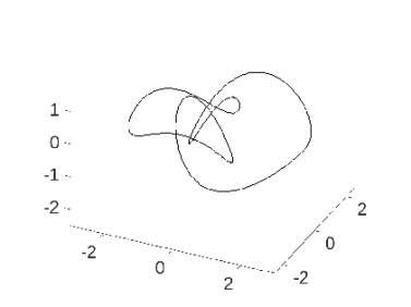
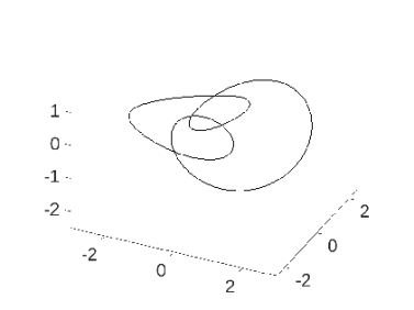
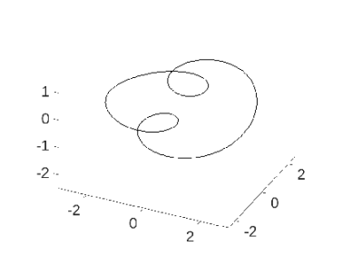
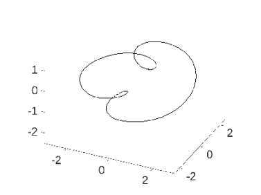
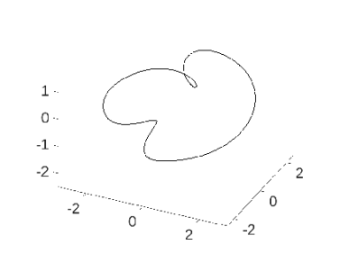
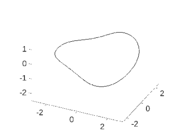
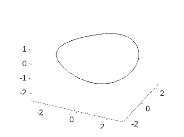
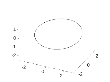
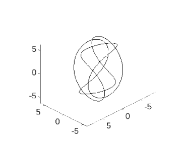
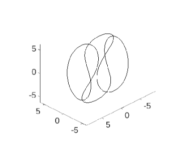
We also present a numerical experiment for $d=3$. To this end, we consider the two interlocked rings in ${\mathbb{R}}^{3}$ from [19, Fig. 4]. In particular, the initial curve is given by

$$x_{0}(\rho)=\tfrac{1}{8}\begin{pmatrix}10(\cos(2\pi\rho)+\cos(6\pi\rho))+\cos(4\pi\rho)+\cos(8\pi\rho)\\ 6\sin(2\pi\rho)+10\sin(6\pi\rho)\\ 4\sin(6\pi\rho)\sin(5\pi\rho)+4\sin(8\pi\rho)-2\sin(12\pi\rho)\end{pmatrix}\quad\rho\in I.$$ (6.5)

The evolution of this curve under curve diffusion can be seen in Figure 4. For this experiment we also include a plot of the inverse of the maximal magnitude of the discrete curvature, (6.2). This strongly indicates that during the shown evolution the curve does not become singular, i.e. the curvature remains bounded. This is in stark contrast to the corresponding evolution under curve shortening flow. In fact, the authors recently numerically studied that particular example in [19, Fig. 4], where the numerical evidence suggests that the flow undergoes a singularity.

Figure 4: Curve diffusion for the two interlocked rings (6.5). We show $\Gamma^{m}$ at times $t=0,1,3,3.5,3.7,4,5,6,T=10$. Below are plots of $|\Gamma^{m}|$ (left), ${\mathfrak{r}}^{m}$ (middle) and $1/K^{m}_{\infty}$ (right) over time.

6.2 Elastic flow

In this section we will monitor the discrete elastic energy

$$E^{m}=\tfrac{1}{2}\int_{I}|P^{m}_{h}y^{m}_{h}|^{2}|x^{m}_{h,\rho}|\;{\rm d}\rho+\lambda\int_{I}|x^{m}_{h,\rho}|\;{\rm d}\rho,$$

where $P^{m}_{h}=I\!d-\frac{x^{m}_{h,\rho}}{|x^{m}_{h,\rho}|}\otimes\frac{x^{m}_{h,\rho}}{|x^{m}_{h,\rho}|}$. Unless otherwise stated we choose $\lambda=0$ for the simulations presented in this section.

We begin with an experiment for a known exact solution. In fact, it is easy to see that

$$x(\rho,t)=(1+2t)^{\frac{1}{4}}\binom{\cos g(\rho)}{\sin g(\rho)},$$ (6.6)

recall (6.4), satisfies (1.4) with $\lambda=0$. We demonstrate the resulting evolution by computing the numerical solution for our scheme (5.4). As can be seen from Figure 5, we see that the circle expands with the prescribed rate. Moreover, we observe that our scheme induces a tangential motion that in this experiment leads to a slightly better distribution of vertices. Hence the discrete functions $x_{h}^{m}$ will in general not approximate the particular parameterizations $x(\cdot,t_{m})$, since these are strictly radial.

Figure 5: Elastic flow with $\lambda=0$ for a circle. We show $\Gamma^{m}$ at times $t=0,0.5,T=1$ (left) and plots of $E^{m}$ (middle) and ${\mathfrak{r}}^{m}$ (right) over time.

Nevertheless, we can use (6.6) to perform a convergence experiment for elastic flow for our scheme (5.4). To this end, we construct the (tangential) right-hand side $f_{el}=|x_{\rho}|^{2}x_{t}+y_{\rho\rho}-F_{el}(x_{\rho},y,y_{\rho})y$, and then add the correction term $\int_{I}\pi^{h}\left[f_{el}(\cdot,t_{m})\cdot\eta_{h}\right]\!\;{\rm d}\rho$ to the right hand side of (5.4a). We then compare the obtained discrete solutions with (6.6). The results are displayed in Table 2, where we once again observe the expected optimal convergence rates, similarly to Table 1.

32	4.3864e-03	—	4.7788e-01	—	5.3851e-02	—	5.2408e-01	—
64	1.0940e-03	2.00	2.3855e-01	1.00	1.2679e-02	2.09	2.0845e-01	1.33
128	2.7343e-04	2.00	1.1923e-01	1.00	3.1339e-03	2.02	9.7576e-02	1.10
256	6.8356e-05	2.00	5.9608e-02	1.00	7.8138e-04	2.00	4.7947e-02	1.03
512	1.7089e-05	2.00	2.9803e-02	1.00	1.9522e-04	2.00	2.3868e-02	1.01

Table 2: Errors for the convergence test for (6.6), with (6.4), over the time interval $[0,1]$. We also display the experimental orders of convergence (EOC).

We now consider an experiment for an elongated tube of total dimension $8\times 1$, as in Figure 1. We can see from Figure 6 that during the elastic flow the curve loses its convexity, while it monotonically decreases its discrete energy. In fact, the curve evolves towards an expanding circle. Moreover, the ratio (6.1) at first increases slightly, before it eventually converges to the optimal value of 1. This indicates that also our scheme (5.4) asymptotically achieves equidistribution in practice.

Figure 6: Elastic flow with $\lambda=0$ for a $8\!:\!1$ tube. We show $\Gamma^{m}$ at times $t=0,1,2,10,20,T=50$ (left) and plots of $E^{m}$ (middle) and ${\mathfrak{r}}^{m}$ (right) over time.

The next experiment is for a $2:1$ lemniscate, and is a repeat of the numerical simulations in [10, Fig. 1]. In particular, we choose $J=100$ and $\Delta t=10^{-4}$ as there, and start from an equidistributed parameterization. We show the results obtained from our scheme (5.4) in Figure 7, and once again observe the smooth evolution with a nice distribution of mesh points throughout. This latter aspect is a clear difference to the corresponding results shown for the scheme from [16] in [10, Fig. 1].

Figure 7: Elastic flow with $\lambda=0$ for a $2\!:\!1$ lemniscate. We show $\Gamma^{m}$ at times $t=0,2,4,T=6$ (left) and plots of $E^{m}$ (middle) and ${\mathfrak{r}}^{m}$ (right) over time.

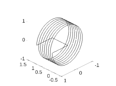
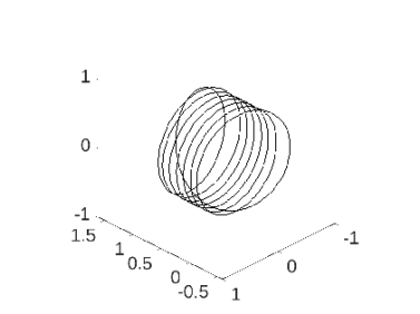
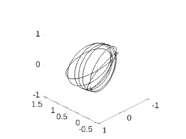
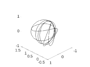
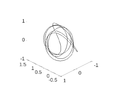
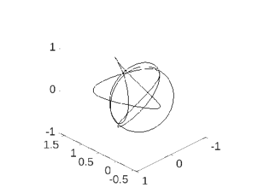
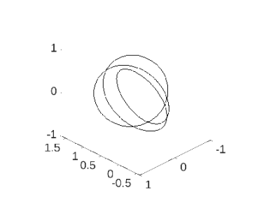
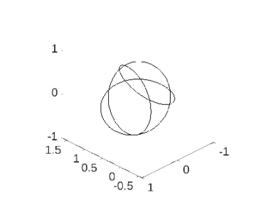
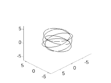
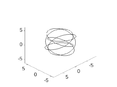
In our next experiment we consider a closed helix in ${\mathbb{R}}^{3}$, as in [8, Figure 2]. Here the open helix is defined by

$$x_{0}(\varrho)=(\sin(16\,\pi\varrho),\cos(16\,\pi\,\varrho),\varrho)^{T}\,,\quad\varrho\in[0,1]\,,$$ (6.7)

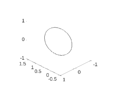
and the initial curve is constructed from (6.7) by connecting $x_{0}(0)$ and $x_{0}(1)$ with a polygon that visits the origin and $(0,0,1)^{T}$. The evolution of the helix under elastic flow with $\lambda=1$ can be seen in Figure 8.

Figure 8: Elastic flow with $\lambda=1$ for the helix (6.7). We show $\Gamma^{m}$ at times $t=0,1,3,4,\ldots,8,T=10$. Below are plots of $E^{m}$ (left) and ${\mathfrak{r}}^{m}$ (right) over time.

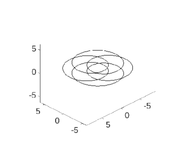
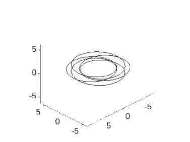
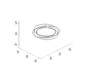
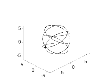
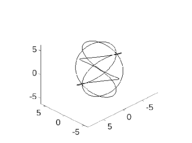
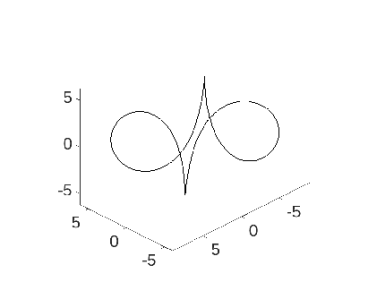
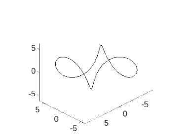
Our final experiments are for the hypocycloid as in [16, Example 4.3]. In particular, we let

$$x_{0}(\rho)=\left(-\tfrac{5}{2}\cos(2\pi\rho)+4\cos(10\pi\rho),-\tfrac{5}{2}\sin(2\pi\rho)+4\sin(10\pi\rho),\delta\sin(6\pi\rho)\right)\quad\rho\in I,$$ (6.8)

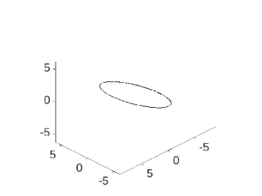
and choose $\lambda=0.025$. For the choice $\delta=0$ the curve remains planar, evolving towards a five-fold covering of a circle. When we choose $\delta=0.1$, on the other hand, the curve eventually begins to unfold and then converges to a single circle. For these experiments we use the larger time step size $\Delta t=10^{-3}$. See Figures 9 and 10 for the results.

Figure 9: Elastic flow with $\lambda=0.025$ for the hypocycloid (6.8) with $\delta=0$. We show $\Gamma^{m}$ at times $t=0,3000,5000,T=10000$. Below are plots of $E^{m}$ (left) and ${\mathfrak{r}}^{m}$ (right) over time.

Figure 10: Elastic flow with $\lambda=0.025$ for the hypocycloid (6.8) with $\delta=0.1$. We show $\Gamma^{m}$ at times $t=0,1700,3000,5000,5500,6000,6500,7300,8000,8500,8700,T=10^{4}$. Below are plots of $E^{m}$ (left) and ${\mathfrak{r}}^{m}$ (right) over time.

Appendix A Appendix

For given functions $x\in H^{2}(I,{\mathbb{R}}^{d}),y\in H^{1}(I,{\mathbb{R}}^{d})$ we define $f:{\mathbb{R}}^{d}\to{\mathbb{R}}^{d}$ by

$$f(c):=F(x_{\rho},y,c)y-F(x_{\rho},y,0)y=2(x_{\rho}\cdot c)y+2(x_{\rho}\cdot y)c-2(y\cdot c)x_{\rho}.$$

Note, that the second equality holds both for $F=F_{cd}$ and $F=F_{el}$, recall (2.10) and (2.13). Clearly, $f$ is linear and it is easily seen that (4.1) holds if and only if $a(R_{h}w,\chi)=a(w,\chi)$ for all $\chi\in\underline{V}^{h}$, where the bilinear form $a:H^{1}(I;{\mathbb{R}}^{d})\times H^{1}(I;{\mathbb{R}}^{d})\rightarrow{\mathbb{R}}$ is given by

$$a(v,\chi):=\int_{I}v_{\rho}\cdot\chi_{\rho}\;{\rm d}\rho+\int_{I}f(v_{\rho})\cdot\chi\;{\rm d}\rho+\gamma\int_{I}v\cdot\chi\;{\rm d}\rho.$$

Lemma. A.1.

Let $x\in H^{2}(I,{\mathbb{R}}^{d}),y\in H^{1}(I,{\mathbb{R}}^{d})$ with $|x_{\rho}|\leq C_{0}$, $|y|\leq C_{0}$ and choose $\gamma\geq 18C_{0}^{4}+\frac{1}{2}$. Then, for every $w\in H^{2}(I;{\mathbb{R}}^{d})$ there exists a unique $R_{h}w\in\underline{V}^{h}$ such that

$$a(R_{h}w,\chi)=a(w,\chi)\qquad\mbox{ for all }\chi\in\underline{V}^{h}$$

and

$$\|w-R_{h}w\|_{0}+h|w-R_{h}w|_{1}\leq Ch^{2}\|w\|_{2}.$$ (A.1a)

Moreover, if $$x\in C^{1}([0,T];H^{2}(I,{\mathbb{R}}^{d})),y\in C^{1}([0,T];H^{1}(I,{\mathbb{R}}^{d})) R_{h}w\in C^{1}([0,T];\underline{V}^{h}) t\in[0,T]$$ then and we have for

$$\|w_{t}(\cdot,t)-(R_{h}w)_{t}(\cdot,t)\|_{0}+h|w_{t}(\cdot,t)-(R_{h}w)_{t}(\cdot,t)|_{1}\leq Ch^{2}\bigl{(}\|w(\cdot,t)\|_{2}+\|w_{t}(\cdot,t)\|_{2}\bigr{)}.$$ (A.1b)

Proof. Clearly, $|f(c)|\leq 6C_{0}^{2}|c|$ so that

$$a(v,v)\geq|v|_{1}^{2}+\gamma\|v\|_{0}^{2}-6C_{0}^{2}|v|_{1}\|v\|_{0}\geq\tfrac{1}{2}\|v\|_{1}^{2},$$

and hence $a$ is elliptic on $H^{1}(I;{\mathbb{R}}^{d})$. The bound on $\|w-R_{h}w\|_{1}$ follows upon inserting $\chi=\pi^{h}w-R_{h}w$ into the orthogonality relation $a(w-R_{h}w,\chi)=0$ and using standard interpolation estimates, see e.g. (3.2b). The $L^{2}$–bound is obtained with the help of the usual duality argument. It is not difficult to see that the dual problem $a(v,z)=\int_{I}v\cdot(w-R_{h}w)\;{\rm d}\rho$ for all $v\in H^{1}(I;{\mathbb{R}}^{d})$ is given by the equation

$$-z_{\rho\rho}-2\bigl{(}(y\cdot z)x_{\rho}\bigr{)}_{\rho}-2\bigl{(}(x_{\rho}\cdot y)z\bigr{)}_{\rho}+2\bigl{(}(x_{\rho}\cdot z)y\bigr{)}_{\rho}+\gamma z=w-R_{h}w\quad\mbox{ in }I.$$

Its solution $z$ belongs to $H^{2}(I;{\mathbb{R}}^{d})$ and satisfies $\|z\|_{2}\leq C\|w-R_{h}w\|_{0}$. The $L^{2}$–bound in (A.1a) is then derived in the usual way. In the case that $x$ and $y$ depend on $t$, the structure of $f$ and integration by parts imply that $(R_{h}w)_{t}(\cdot,t)$ is a solution of the problem

$$a((R_{h}w)_{t}(\cdot,t),\chi)=a(w_{t}(\cdot,t),\chi)+b\bigl{(}(w-R_{h}w)(\cdot,t),\chi\bigr{)}\qquad\mbox{ for all }\chi\in\underline{V}^{h},$$

where the bilinear form $b$ satisfies

$$|b\bigl{(}(w-R_{h}w)(\cdot,t),\chi\bigr{)}|\leq C\|(w-R_{h}w)(\cdot,t)\|_{0}\|\chi\|_{1}\leq Ch^{2}\|w(\cdot,t)\|_{2}\|\chi\|_{1}$$

in view of (A.1a). The bound (A.1b) is now obtained in a similar way as before.      

Lemma. A.2.

Let $x_{0}\in H^{4}(I,{\mathbb{R}}^{d})$ such that $x_{0,\rho}\neq 0$ in $I$ and set $y_{0}=\frac{x_{0,\rho\rho}}{|x_{0,\rho}|^{2}}$. Let $\widehat{x}^{0}_{h}\in\underline{V}^{h}$ be the solution of (3.6) and $\widehat{y}_{h}^{0}\in\underline{V}^{h}$ the solution of (3.8) respectively. Then there exists $h_{0}>0$ such that there holds for $0<h\leq h_{0}$

$$\|\pi^{h}x_{0}-\widehat{x}^{0}_{h}\|_{1}+\|y_{0}-\widehat{y}^{0}_{h}\|_{0}\leq Ch^{2}.$$ (A.2)

Proof. It follows from (3.3) that for all $\eta\in\underline{V}^{h}\subset H^{1}(I,{\mathbb{R}}^{d})$ it holds that

$$\int_{I}(\pi^{h}x_{0})_{\rho}\cdot\eta_{\rho}\;{\rm d}\rho=\int_{I}x_{0,\rho}\cdot\eta_{\rho}\;{\rm d}\rho=-\int_{I}x_{0,\rho\rho}\cdot\eta\;{\rm d}\rho=-\int_{I}y_{0}\cdot\eta|x_{0,\rho}|^{2}\;{\rm d}\rho.$$

Taking the difference of this relation with (3.6) we obtain

$$\int_{I}(\pi^{h}x_{0}-\widehat{x}^{0}_{h})_{\rho}\cdot\eta_{\rho}\;{\rm d}\rho+\int_{I}(\pi^{h}x_{0}-\widehat{x}^{0}_{h})\cdot\eta\;{\rm d}\rho$$

$$\quad=\int_{I}(\pi^{h}y_{0}-y_{0})\cdot\eta|(\pi^{h}x_{0})_{\rho}|^{2}\;{\rm d}\rho+\int_{I}y_{0}\cdot\eta\bigl{[}|(\pi^{h}x_{0})_{\rho}|^{2}-|x_{0,\rho}|^{2}\bigr{]}\;{\rm d}\rho$$

$$\quad=\int_{I}(\pi^{h}y_{0}-y_{0})\cdot\eta|(\pi^{h}x_{0})_{\rho}|^{2}\;{\rm d}\rho$$

$$\qquad+\int_{I}y_{0}\cdot\eta|(\pi^{h}x_{0}-x_{0})_{\rho}|^{2}\;{\rm d}\rho-2\int_{I}y_{0}\cdot\eta\bigl{[}x_{0,\rho}\cdot(x_{0}-\pi^{h}x_{0})_{\rho}\bigr{]}\;{\rm d}\rho.$$

Choosing $\eta=\pi^{h}x_{0}-\widehat{x}^{0}_{h}$ and using integration by parts for the last integral we deduce the first bound in (A.2) from (3.2b). Next, combining (3.6) and (3.8) we obtain

$$\int_{I}\widehat{y}_{h}^{0}\cdot\eta|\widehat{x}^{0}_{h,\rho}|^{2}\;{\rm d}\rho=\int_{I}(\widehat{x}^{0}_{h}-\pi^{h}x_{0})\cdot\eta\;{\rm d}\rho+\int_{I}\pi^{h}y_{0}\cdot\eta|(\pi^{h}x_{0})_{\rho}|^{2}\;{\rm d}\rho$$

and hence

$$\int_{I}(y_{0}-\widehat{y}_{h}^{0})\cdot\eta|\widehat{x}^{0}_{h,\rho}|^{2}\;{\rm d}\rho=\int_{I}(y_{0}-\pi^{h}y_{0})\cdot\eta|\widehat{x}^{0}_{h,\rho}|^{2}\;{\rm d}\rho$$

$$\quad+\int_{I}(\pi^{h}x_{0}-\widehat{x}^{0}_{h})\cdot\eta\;{\rm d}\rho+\int_{I}\pi^{h}y_{0}\cdot\eta\bigl{[}|\widehat{x}^{0}_{h,\rho}|^{2}-|(\pi^{h}x_{0})_{\rho}|^{2}\bigr{]}\;{\rm d}\rho.$$

Using that $\|\pi^{h}x_{0}-\widehat{x}^{0}_{h}\|_{1}\leq Ch^{2}$ we infer that there exists $h_{0}>0$ such that $\frac{1}{2}c_{0}\leq|\widehat{x}^{0}_{h,\rho}|\leq 2C_{0}$ for $0<h\leq h_{0}$. If we now choose $\eta=\pi^{h}y_{0}-\widehat{y}_{h}^{0}$ and use again the bound on $\pi^{h}x_{0}-\widehat{x}^{0}_{h}$ we deduce the second estimate in (A.2) in a straightforward manner.

References

- [1] E. Bänsch, K. Deckelnick, H. Garcke, and P. Pozzi, Interfaces: Modeling, Analysis, Numerics, vol. 51 of Oberwolfach Seminars, Birkhäuser/Springer, Cham, 2023.
- [2] E. Bänsch, P. Morin, and R. H. Nochetto, Surface diffusion of graphs: variational formulation, error analysis, and simulation, SIAM J. Numer. Anal., 42 (2004), pp. 773–799.
- [3] , A finite element method for surface diffusion: the parametric case, J. Comput. Phys., 203 (2005), pp. 321–343.
- [4] W. Bao and Y. Li, An energy-stable parametric finite element method for the planar Willmore flow. arXiv:2401.13274, 2024.
- [5] W. Bao and Q. Zhao, A structure-preserving parametric finite element method for surface diffusion, SIAM J. Numer. Anal., 59 (2021), pp. 2775–2799.
- [6] J. W. Barrett, H. Garcke, and R. Nürnberg, A parametric finite element method for fourth order geometric evolution equations, J. Comput. Phys., 222 (2007), pp. 441–462.
- [7] , Parametric approximation of Willmore flow and related geometric evolution equations, SIAM J. Sci. Comput., 31 (2008), pp. 225–253.
- [8] , Numerical approximation of gradient flows for closed curves in , IMA J. Numer. Anal., 30 (2010), pp. 4–60.
- [9] , The approximation of planar curve evolutions by stable fully implicit finite element schemes that equidistribute, Numer. Methods Partial Differential Equations, 27 (2011), pp. 1–30.
- [10] , Parametric approximation of isotropic and anisotropic elastic flow for closed and open curves, Numer. Math., 120 (2012), pp. 489–542.
- [11] , Parametric finite element approximations of curvature driven interface evolutions, in Handb. Numer. Anal., A. Bonito and R. H. Nochetto, eds., vol. 21, Elsevier, Amsterdam, 2020, pp. 275–423.
- [12] S. Bartels, A simple scheme for the approximation of the elastic flow of inextensible curves, IMA J. Numer. Anal., 33 (2013), pp. 1115–1125.
- [13] F. Davi and M. E. Gurtin, On the motion of a phase interface by surface diffusion, Z. Angew. Math. Phys., 41 (1990), pp. 782–811.
- [14] T. A. Davis, Algorithm 832: UMFPACK V4.3—an unsymmetric-pattern multifrontal method, ACM Trans. Math. Software, 30 (2004), pp. 196–199.
- [15] K. Deckelnick and G. Dziuk, On the approximation of the curve shortening flow, in Calculus of Variations, Applications and Computations (Pont-à-Mousson, 1994), C. Bandle, J. Bemelmans, M. Chipot, J. S. J. Paulin, and I. Shafrir, eds., vol. 326 of Pitman Res. Notes Math. Ser., Longman Sci. Tech., Harlow, 1995, pp. 100–108.
- [16] , Error analysis for the elastic flow of parametrized curves, Math. Comp., 78 (2009), pp. 645–671.
- [17] K. Deckelnick, G. Dziuk, and C. M. Elliott, Error analysis of a semidiscrete numerical scheme for diffusion in axially symmetric surfaces, SIAM J. Numer. Anal., 41 (2003), pp. 2161–2179.
- [18] , Computation of geometric partial differential equations and mean curvature flow, Acta Numer., 14 (2005), pp. 139–232.
- [19] K. Deckelnick and R. Nürnberg, Discrete anisotropic curve shortening flow in higher codimension. arXiv:2310.02138, 2023.
- [20] W. Dörfler and R. Nürnberg, Discrete gradient flows for general curvature energies, SIAM J. Sci. Comput., 41 (2019), pp. 2012–2036.
- [21] B. Duan and B. Li, New artificial tangential motions for parametric finite element approximation of surface evolution, SIAM J. Sci. Comput., 46 (2024), pp. 587–608.
- [22] G. Dziuk, E. Kuwert, and R. Schätzle, Evolution of elastic curves in : Existence and computation, SIAM J. Math. Anal., 33 (2002), pp. 1228–1245.
- [23] C. M. Elliott and H. Fritz, On approximations of the curve shortening flow and of the mean curvature flow based on the DeTurck trick, IMA J. Numer. Anal., 37 (2017), pp. 543–603.
- [24] C. M. Elliott and H. Garcke, Existence results for diffusive surface motion laws, Adv. Math. Sci. Appl., 7 (1997), pp. 465–488.
- [25] J. Escher, U. F. Mayer, and G. Simonett, The surface diffusion flow for immersed hypersurfaces, SIAM J. Math. Anal., 29 (1998), pp. 1419–1433.
- [26] M. Gage and R. S. Hamilton, The heat equation shrinking convex plane curves, J. Differential Geom., 23 (1986), pp. 69–96.
- [27] Y. Giga and K. Ito, On pinching of curves moved by surface diffusion, Commun. Appl. Anal., 2 (1998), pp. 393–405.
- [28] , Loss of convexity of simple closed curves moved by surface diffusion, in Topics in nonlinear analysis, vol. 35 of Progr. Nonlinear Differential Equations Appl., Birkhäuser, Basel, 1999, pp. 305–320.
- [29] S. Goyal, N. C. Perkins, and C. L. Lee, Nonlinear dynamics and loop formation in Kirchhoff rods with implications to the mechanics of DNA and cables, J. Comput. Phys., 209 (2005), pp. 371–389.
- [30] M. A. Grayson, The heat equation shrinks embedded plane curves to round points, J. Differential Geom., 26 (1987), pp. 285–314.
- [31] W. Jiang and B. Li, A perimeter-decreasing and area-conserving algorithm for surface diffusion flow of curves, J. Comput. Phys., 443 (2021), pp. Paper No. 110531, 11.
- [32] C.-C. Lin and H. R. Schwetlick, On the geometric flow of Kirchhoff elastic rods, SIAM J. Appl. Math., 65 (2004), pp. 720–736.
- [33] K. Mikula and D. Ševčovič, Tangentially stabilized Lagrangian algorithm for elastic curve evolution driven by intrinsic Laplacian of curvature, in ALGORITMY 2005, A. Handlovicova, Z. Kriva, K. Mikula, and D. Ševčovič, eds., Bratislava, 2005, Slovak University of Technology, pp. 32–41.
- [34] W. W. Mullins, Theory of thermal grooving, J. Appl. Phys., 28 (1957), pp. 333–339.
- [35] A. Polden, Curves and surfaces of least total curvature and fourth-order flows, PhD thesis, University Tübingen, Tübingen, 1996.
- [36] P. Pozzi and B. Stinner, Convergence of a scheme for an elastic flow with tangential mesh movement, ESAIM Math. Model. Numer. Anal., 57 (2023), pp. 445–466.
- [37] A. Schmidt and K. G. Siebert, Design of Adaptive Finite Element Software: The Finite Element Toolbox ALBERTA, vol. 42 of Lecture Notes in Computational Science and Engineering, Springer-Verlag, Berlin, 2005.
- [38] J. E. Taylor and J. W. Cahn, Linking anisotropic sharp and diffuse surface motion laws via gradient flows, J. Statist. Phys., 77 (1994), pp. 183–197.
- [39] Z. C. Tu and Z. C. Ou-Yang, Elastic theory of low-dimensional continua and its applications in bio- and nano-structures, J. Comput. Theor. Nanosci., 5 (2008), pp. 422–448.
- [40] Y. Wen, Curve straightening flow deforms closed plane curves with nonzero rotation number to circles, J. Differential Equations, 120 (1995), pp. 89–107.