Convergence analysis for a fully-discrete finite element approximation of the unsteady $p(\cdot,\cdot)$-Navier–Stokes equations

Abstract

In the present paper, we establish the well-posedness, stability, and (weak) convergence of a fully-discrete approximation of the unsteady $p(\cdot,\cdot)$-Navier–Stokes equations employing an implicit Euler step in time and a discretely inf-sup-stable finite element approximation in space. Moreover, numerical experiments are carried out that supplement the theoretical findings.

Keywords:   Variable exponents; convergence analysis; velocity; pressure; Rothe method; Galerkin method; finite elements.

AMS MSC (2020):    35Q35; 65M12; 65N30; 76A05.

1.  Introduction

In this paper, we examine a fully-discrete Rothe–Galerkin approximation for unsteady systems of $p(\cdot,\cdot)$-Navier–Stokes type, i.e.,

$$\partial_{t}\boldsymbol{v}-\mathrm{div}_{x}(\mathbf{S}(\cdot,\cdot,\mathbf{D}_{x}\boldsymbol{v}))+\mathrm{div}_{x}(\boldsymbol{v}\otimes\boldsymbol{v})+\nabla_{\!x}\pi =\boldsymbol{f}+\mathrm{div}_{x}\boldsymbol{F} \quad\text{ in }Q_{T}\,,$$ (1.1)

$$\mathrm{div}_{x}\boldsymbol{v} =0 \quad\text{ in }Q_{T}\,,$$

$$\boldsymbol{v} =\mathbf{0} \quad\text{ on }\Gamma_{T}\,,$$

$$\boldsymbol{v}(0) =\mathbf{v}_{0} \quad\text{ in }\Omega\,,$$

using an implicit Euler step in time and a discretely inf-sup-stable finite element approximation in space. More precisely, for a given vector field $\boldsymbol{f}\colon Q_{T}\to\mathbb{R}^{d}$ and a given tensor field $\boldsymbol{F}\colon Q_{T}\to\mathbb{R}^{d\times d}_{\mathrm{sym}}$, jointly describing external body forces, an incompressibility constraint (1.1)₂, a no-slip boundary condition (1.1)₃, and an initial velocity vector field $\mathbf{v}_{0}\colon\Omega\to\mathbb{R}^{d}$ at initial time $t=0$, the system (1.1) seeks for a velocity vector field $\boldsymbol{v}\coloneqq(v_{1},\ldots,v_{d})^{\top}\colon\overline{Q_{T}}\to\mathbb{R}^{d}$ and a scalar kinematic pressure ${\pi\colon Q_{T}\to\mathbb{R}}$ solving (1.1). Here, $\Omega\subseteq\mathbb{R}^{d}$, $d\geq 2$, is a bounded simplicial Lipschitz domain, $I\coloneqq(0,T)$, $0<T<\infty$, a finite time interval, $Q_{T}\coloneqq I\times\Omega$ the corresponding time-space cylinder and $\Gamma_{T}\coloneqq I\times\partial\Omega$ the parabolic boundary. The extra-stress tensor $\mathbf{S}(\cdot,\cdot,\mathbf{D}_{x}\boldsymbol{v})\colon Q_{T}\to\mathbb{R}^{d\times d}_{\textup{sym}}$ depends on the strain-rate tensor $\smash{\mathbf{D}_{x}\boldsymbol{v}\coloneqq[\nabla_{\!x}\boldsymbol{v}]^{\textup{sym}}\colon Q_{T}\to\mathbb{R}^{d\times d}_{\textup{sym}}}$, i.e., the symmetric part of the velocity gradient $\nabla_{\!x}\boldsymbol{v}=(\partial_{x_{j}}v_{i})_{i,j=1,\ldots,d}\colon Q_{T}\to\mathbb{R}^{d\times d}$. The convective term ${\mathrm{div}_{x}(\boldsymbol{v}\otimes\boldsymbol{v})\colon Q_{T}\to\mathbb{R}^{d}}$ is defined by $(\mathrm{div}_{x}(\boldsymbol{v}\otimes\boldsymbol{v}))_{i}\coloneqq\sum_{j=1}^{d}{\partial_{x_{j}}(v_{i}v_{j})}$ for all $i=1,\ldots,d$.

Throughout the paper, we assume that the extra-stress tensor $\mathbf{S}$ has a weak $(p(\cdot,\cdot),\delta)$-structure, i.e., for some $\delta\geq 0$ and some power-law index $p\colon Q_{T}\to[0,+\infty)$, which is at least (Lebesgue) measurable with

$$1<p^{-}\coloneqq\underset{(t,x)^{\top}\in Q_{T}}{\textrm{ess\,inf}}{p(t,x)}\leq p^{+}\coloneqq\underset{(t,x)^{\top}\in Q_{T}}{\textrm{ess\,sup}}{p(t,x)}<+\infty\,,$$ (1.2)

the following properties are satisfied:

• $\textbf{S}\colon Q_{T}\times\mathbb{R}^{d\times d}_{\textup{sym}}\to\mathbb{R}^{d\times d}_{\textup{sym}}$ is a Carathéodory mapping;

• $|\mathbf{S}(t,x,\mathbf{A})|\leq\alpha\,(\delta+|\mathbf{A}|)^{p(t,x)-2}|\mathbf{A}|+\beta(t,x)$ for all $\mathbf{A}\in\mathbb{R}^{d\times d}_{\textup{sym}}$ and a.e.  $(t,x)^{\top}\in Q_{T}$,
  where $\alpha\geq 1$ and $\beta\in L^{p^{\prime}(\cdot,\cdot)}(Q_{T};\mathbb{R}_{\geq 0})$;

• $\mathbf{S}(t,x,\mathbf{A}):\mathbf{A}\geq c_{0}\,(\delta+|\mathbf{A}|)^{p(t,x)-2}|\mathbf{A}|^{2}-c_{1}(t,x)$ for all ${\mathbf{A}\in\mathbb{R}^{d\times d}_{\textup{sym}}}$ and a.e. ${(t,x)^{\top}\in Q_{T}}$,
  where $c_{0}>0$ and $c_{1}\in L^{1}(Q_{T};\mathbb{R}_{\geq 0})$;

• $(\mathbf{S}(t,x,\mathbf{A})-\mathbf{S}(t,x,\mathbf{B})):(\mathbf{A}-\mathbf{B})\geq 0$ for all $\mathbf{A},\mathbf{B}\in\mathbb{R}^{d\times d}_{\textup{sym}}$ and a.e.  $(t,x)^{\top}\in Q_{T}$.

A prototypical example for $\textbf{S}\colon Q_{T}\times\mathbb{R}^{d\times d}_{\textup{sym}}\to\mathbb{R}^{d\times d}_{\textup{sym}}$ satisfying (S.1)–(S.1), for a.e.  $(t,x)^{\top}\in Q_{T}$ and every $\mathbf{A}\in\smash{\mathbb{R}^{d\times d}_{\textup{sym}}}$, is defined by

$$\smash{\mathbf{S}(t,x,\mathbf{A})\coloneqq\mu_{0}\,(\delta+|\mathbf{A}|)^{p(t,x)-2}\mathbf{A}\,,}$$ (1.3)

where $\mu_{0}>0$, $\delta\geq 0$, and the power-law index $p\colon Q_{T}\to[0,+\infty)$ is at least (Lebesgue) measurable with (1.2).

The unsteady $p(\cdot,\cdot)$-Navier–Stokes equations (1.1) is a prototypical example of a non-linear system with variable growth conditions. It appears naturally in physical models for smart fluids, e.g., electro-rheological fluids (cf. [47, 49]), micro-polar electro-rheological fluids (cf. [27, 28]), magneto-rheological fluids (cf. [16]), chemically reacting fluids (cf. [41, 15, 40]), and thermo-rheological fluids (cf. [55, 4]). In all these models, the power-law index $p(\cdot,\cdot)$ is a function depending on certain physical quantities, e.g., an electric field, a magnetic field, a concentration field of a chemical material or a temperature field, and, consequently, implicitly depends on $(t,x)^{\top}\in Q_{T}$. Smart fluids have the potential for an application in various areas, such as, e.g., in electronic, automobile, heavy machinery, military, and biomedical industry (cf. [7, Chap. 6] for an overview).

Related contributions

We recall known analytical and numerical results for the unsteady $p(\cdot,\cdot)$-Navier–Stokes equations (1.1).

Existence analyses

The existence analysis of the unsteady $p(\cdot,\cdot)$-Navier–Stokes equations (1.1) is by now well-understood and developed essentially in the following main steps:

• In [49], deploying the $A$-approximation technique, M. Růžička proved the weak solvability of (1.1) for

  $$p\in C^{1}(\overline{Q_{T}})\quad\text{ with }\quad 2\leq p^{-}\leq p^{+}<\min\Big{\{}\frac{8}{3},\frac{3+p^{-}}{2(3-p^{-})}\Big{\}}\,;$$

• In [56, 45], by means of hydro-mechanical Parabolic Compensated Compactness Principles (PCCPs), V. V. Zhikov and S. E. Pastukhova proved the weak solvability of (1.1) for

  $$p\in L^{\infty}(Q_{T})\text{ with }p(t,\cdot)\in\mathcal{P}^{\log}(\Omega)\text{ for a.e.\ }t\in I\quad\text{ and }\quad\frac{3d}{d+2}<p^{-}\leq p^{+}<\min\Big{\{}p^{-}+2,p^{-}\frac{d+2}{d}\Big{\}}\,;$$

• In [39], combining a generalized parabolic pseudo-monotonicity theory with the PCCPs in [56, 45], the weak solvability of (1.1) was proved for

  $$p\in\mathcal{P}^{\log}(Q_{T})\quad\text{ with }\quad p^{-}>\frac{3d}{d+2}\,;$$

• In [17], M. Buliček et al. proved the weak solvability of (1.1) for

  $$p\in L^{\infty}(Q_{T})\text{ with }p(t,\cdot)\in\mathcal{P}^{\log}(\Omega)\text{ for a.e.\ }t\in I\,,\quad\textrm{ess\,sup}_{t\in I}{c_{\log}(p(t,\cdot))}<\infty\,,\quad\text{ and }\quad p^{-}\geq\frac{3d+2}{d+2}\,.$$

Apart from that, in [13], in the case of space periodic boundary conditions, D. Breit and F. Gemeinder proved the weak solvability of (1.1) for $p\in W^{1,\infty}(Q_{T})$ with $p^{-}>\frac{3d}{d+2}$.

Numerical analyses

On the contrary, the numerical analysis of unsteady problems with variable exponents non-linearity is less developed and we are only aware of the following contributions treating the unsteady case:

• The first semi-discrete (i.e., discrete-in-time) numerical analysis of the unsteady $p(\cdot,\cdot)$-Navier–Stokes equations (1.1) goes back to L. Diening (cf. [22]).

• The first fully-discrete (i.e., discrete-in-time and -space) numerical analysis of the unsteady $p(\cdot,\cdot)$-Navier–Stokes equations (1.1) goes back to E. Carelli et al. (cf. [18]), but considers solely a time-independent power-law index which is less realistic for the models for smart fluids mentioned above. More precisely, in [18], the (weak) convergence of a fully-discrete Rothe–Galerkin approximation to the unsteady $p(\cdot)$-Navier–Stokes equations (1.1) was established employing a regularized convective term and continuous approximations $(p_{h})_{h>0}\subseteq C^{0}(\overline{\Omega})$ satisfying $p_{h}\to p$ in $C^{0}(\overline{\Omega})$ $(h\to 0)$ and $p_{h}\geq p$ in $\overline{\Omega}$ for all $h>0$, which is restrictive in applications.

• In [14], D. Breit and P. R. Mensa derived a priori error estimates for a fully-discrete Rothe–Galerkin approximation of parabolic systems with variable growth conditions without divergence constraint like (1.1)₂ or lower-order terms like the convective term.

New contributions of the paper

The purpose of this paper is to improve the literature with respect to several aspects and, in this way, to establish a firm foundation for further numerical analyses of related complex models involving the unsteady $p(\cdot,\cdot)$-Navier–Stokes equations (1.1) such as, e.g., electro-rheological fluids (cf. [47, 49]), magneto-rheological fluids (cf. [16]), micro-polar electro-rheological fluids (cf. [27, 28]), chemically reacting fluids (cf. [41, 15]), and thermo-rheological fluids (cf. [55, 4]):

• Time-dependency of the power-law index: In this paper, we treat a power-law index $p(\cdot,\cdot)$ that is both time- and space-dependent, which makes the extraction of compactness properties more difficult.

• Discretization of the power-law index: In this paper, we allow arbitrary uniform approximations of the power-law index $p(\cdot,\cdot)$, i.e., we only require that $(p_{h})_{h>0}\subseteq L^{\infty}(Q_{T})$ with $p_{h}\to p$ in $L^{\infty}(Q_{T})$ $(h\to 0)$.

• Unregularized scheme: In this paper, we consider the unregularized convective term. This leads to the restriction $p^{-}>\smash{\frac{3d+2}{d+2}}$. Deploying a regularized convective term, allows us to treat the case $p^{-}\geq 2$. However, then one needs to perform a two-level passage to the limit: first, one passes to the limit with the discretization parameters of the fully-discrete Rothe–Galerkin approximation, in this way, approximating the regularized continuous problem; second, one passes to the limit with the regularization. As there is no parabolic Lipschitz truncation technique available (cf. [39, Sec. 6.3]), the second passage to the limit is still an open problem for the unsteady $p(\cdot,\cdot)$-Navier–Stokes equations (1.1). Therefore, we approximate the unsteady $p(\cdot,\cdot)$-Navier–Stokes equations (1.1) with a single passage to the limit.

• Numerical experiments: Since the weak convergence of a fully-discrete Rothe–Galerkin approximation is difficult to measure in numerical experiments, we carry out numerical experiments for low regularity data. More precisely, we construct solutions with fractional regularity, gradually reduce the fractional regularity parameters, and measure convergence rates that reduce with decreasing (but are stable for fixed) value of the fractional regularity parameters to get an indication that weak convergence is likely.

This paper is organized as follows: In Section 2, we introduce the used notation, recall the definitions of variable Lebesgue spaces and variable Sobolev spaces, and collect auxiliary results. In Section 3, we introduce variable Bochner–Lebesgue spaces and variable Bochner–Sobolev spaces, and collect auxiliary results. In Section 4, we examine the behavior of the weak topologies of variable Lebesgue spaces and variable Bochner–Lebesgue spaces with respect to converging sequences of variable exponents. In Section 5, we introduce the discrete spaces and projectors used in the fully-discrete Rothe-Galerkin approximation. In Section 6, we introduce the concept of non-conforming Bochner condition (M). In Section 7, we specify a general fully-discrete Rothe–Galerkin approximation and establish its well-posedness, stability, and (weak) convergence. In Section 8, we apply the general framework of Section 7 to prove the two main results of the paper, i.e., the well-posedness, stability, and (weak) convergence of a fully-discrete Rothe–Galerkin approximation of the unsteady $p(\cdot,\cdot)$-Stokes equations (i.e., (1.1) without convective term) (cf. Theorem 8.3) and of the unsteady $p(\cdot,\cdot)$-Navier–Stokes equations (1.1) (cf. Theorem 8.5). In Section 9, we complement the theoretical findings with some numerical experiments.

2.  Preliminaries

Throughout the entire paper, let $\Omega\subseteq\mathbb{R}^{d}$, $d\geq 2$, be a bounded simplicial Lipschitz domain, ${I\coloneqq(0,T)}$, $0<T<\infty$, a finite time interval, and $Q_{T}\coloneqq I\times\Omega$ the corresponding time cylinder. The integral mean of a (Lebesgue) integrable function, vector or tensor field $\mathbf{u}\colon M\to\mathbb{R}^{\ell}$, $\ell\in\mathbb{N}$, over a (Lebesgue) measurable set $M\subseteq\mathbb{R}^{n}$, $n\in\mathbb{N}$, with $|M|>0$ is denoted by $\langle\mathbf{u}\rangle_{M}\coloneqq\smash{\frac{1}{|M|}\int_{M}\mathbf{u}\,\textup{d}x}$. For (Lebesgue) measurable functions, vector or tensor fields $\mathbf{u},\mathbf{w}\colon M\to\mathbb{R}^{\ell}$, $\ell\in\mathbb{N}$, and a (Lebesgue) measurable set $M\subseteq\mathbb{R}^{n}$, ${n\in\mathbb{N}}$, we write $(\mathbf{u},\mathbf{w})_{M}\coloneqq\int_{M}\mathbf{u}\odot\mathbf{w}\,\textup{d}x$, whenever the right-hand side is well-defined, where ${\odot\colon\mathbb{R}^{\ell}\times\mathbb{R}^{\ell}\to\mathbb{R}}$ either denotes scalar multiplication, the Euclidean inner product or the Frobenius inner product.

Variable Lebesgue spaces and variable Sobolev spaces

In this section, we summarize all essential information concerning variable Lebesgue spaces and variable Sobolev spaces, which will find use in the hereinafter analysis. For an extensive presentation, we refer the reader to the textbooks [25, 21].

Let $M\subseteq\mathbb{R}^{n}$, $n\in\mathbb{N}$, be a (Lebesgue) measurable set and denote the set of (Lebesgue) measurable functions, vector or tensor fields defined in $M$ by $L^{0}(M;\mathbb{R}^{\ell})$, $\ell\in\mathbb{N}$. A function $p\in L^{0}(M;\mathbb{R}^{1})$ is called variable exponent if $p\geq 1$ a.e. in $M$ and the set of variable exponents is denoted by $\mathcal{P}(M)$. For $p\in\mathcal{P}(M)$, we denote by ${p^{+}\coloneqq\textup{ess\,sup}_{x\in M}{p(x)}}$ and ${p^{-}\coloneqq\textup{ess\,inf}_{x\in M}{p(x)}}$ its constant limit exponents. Then, the set of bounded variable exponents is defined by $\mathcal{P}^{\infty}(M)\coloneqq\{p\in\mathcal{P}(M)\mid p^{+}<\infty\}$. For ${p\in\mathcal{P}^{\infty}(M)}$ and $\mathbf{u}\in L^{0}(M;\mathbb{R}^{\ell})$, $\ell\in\mathbb{N}$, we define the modular (with respect to $p$) by

$$\rho_{p(\cdot),M}(\mathbf{u})\coloneqq\int_{M}{|\mathbf{u}(x)|^{p(x)}\,\mathrm{d}x}\,.$$

Then, for $p\in\mathcal{P}^{\infty}(M)$ and $\ell\in\mathbb{N}$, the variable Lebesgue space is defined by

$$\smash{L^{p(\cdot)}(M;\mathbb{R}^{\ell})\coloneqq\big{\{}\mathbf{u}\in L^{0}(M;\mathbb{R}^{\ell})\mid\rho_{p(\cdot),M}(\mathbf{u})<\infty\big{\}}\,.}$$

In the special case $\ell=1$, we abbreviate $L^{p(\cdot)}(M)\coloneqq L^{p(\cdot)}(M;\mathbb{R}^{1})$. The Luxembourg norm, i.e.,

$$\|\mathbf{u}\|_{p(\cdot),M}\coloneqq\inf\Big{\{}\lambda>0\;\Big{|}\;\rho_{p(\cdot),M}\Big{(}\frac{\mathbf{u}}{\lambda}\Big{)}\leq 1\Big{\}}\,,$$

turns $L^{p(\cdot)}(M;\mathbb{R}^{\ell})$ into a Banach space (cf. [25, Thm.  3.2.7]).

For $p\in\mathcal{P}^{\infty}(M)$ with $p^{-}>1$, $p^{\prime}\coloneqq\frac{p}{p-1}\in\mathcal{P}^{\infty}(M)$ is the conjugate exponent. Then, for $p\in\mathcal{P}^{\infty}(M)$ with $p^{-}>1$ and $\ell\in\mathbb{N}$, we make frequent use of the variable (exponent) Hölder inequality, i.e.,

$$\|\mathbf{u}\odot\mathbf{w}\|_{1,M}\leq 2\,\|\mathbf{u}\|_{p^{\prime}(\cdot),M}\|\mathbf{w}\|_{p(\cdot),M}\,,$$ (2.1)

valid for all $\mathbf{u}\in\smash{L^{p^{\prime}(\cdot)}(M;\mathbb{R}^{\ell})}$ and $\mathbf{w}\in\smash{L^{p(\cdot)}(M;\mathbb{R}^{\ell})}$ (cf. [25, Lem.  3.2.20]), where $\odot\colon\mathbb{R}^{\ell}\times\mathbb{R}^{\ell}\to\mathbb{R}$ either denotes scalar multiplication, the Euclidean inner product or the Frobenius inner product.

For a bounded (Lebesgue) measurable set $M\subseteq\mathbb{R}^{n}$, $n\in\mathbb{N}$, $q,p\in\mathcal{P}^{\infty}(M)$ with $q\leq p$ a.e.  in $M$, and $\ell\in\mathbb{N}$, every $\mathbf{u}\in L^{p(\cdot)}(M;\mathbb{R}^{\ell})$ satisfies $\mathbf{u}\in L^{q(\cdot)}(M;\mathbb{R}^{\ell})$ (cf. [25, Cor. 3.3.4]) with

$$\|\mathbf{u}\|_{q(\cdot),M}\leq 2\,(1+|M|)\,\|\mathbf{u}\|_{p(\cdot),M}\,.$$ (2.2)

For $q,p\in\mathcal{P}^{\infty}(\Omega)$, the symmetric variable Sobolev space is defined by

$$E^{q(\cdot),p(\cdot)}\coloneqq\big{\{}\mathbf{u}\in L^{q(\cdot)}(\Omega;\mathbb{R}^{d})\mid\mathbf{D}_{x}\mathbf{u}\in L^{p(\cdot)}(\Omega;\mathbb{R}^{d\times d}_{\textup{sym}})\big{\}}\,.$$

The symmetric variable Sobolev norm, i.e.,

$$\|\cdot\|_{q(\cdot),p(\cdot),\Omega}\coloneqq\|\cdot\|_{q(\cdot),\Omega}+\|\mathbf{D}_{x}(\cdot)\|_{p(\cdot),\Omega}\,,$$

turns $E^{q(\cdot),p(\cdot)}$ into a Banach space (cf.  [39, Prop.  2.9]). Then, the closure of $C^{\infty}_{c}(\Omega;\mathbb{R}^{d})$ in $E^{q(\cdot),p(\cdot)}$ is denoted by $\smash{E^{q(\cdot),p(\cdot)}_{0}}$, the closure of

$$\mathcal{V}\coloneqq\big{\{}\boldsymbol{\varphi}\in C^{\infty}_{c}(\Omega;\mathbb{R}^{d})\mid\textup{div}_{x}\boldsymbol{\varphi}=0\textup{ in }\Omega\big{\}}$$

in $E^{q(\cdot),p(\cdot)}$ is denoted by $E^{q(\cdot),p(\cdot)}_{0,\textup{div}_{x}}$, and the closure of $\mathcal{V}$ in $Y\coloneqq L^{2}(\Omega;\mathbb{R}^{d})$ is denoted by $H$.

3.  Variable Bochner–Lebesgue spaces and variable Bochner–Sobolev spaces

In this section, we recall the definitions and discuss properties of variable Bochner–Lebesgue spaces and variable Bochner–Sobolev spaces, the appropriate substitutes of classical Bochner–Lebesgue spaces and classical Bochner–Sobolev spaces for the treatment of the unsteady $p(\cdot,\cdot)$-Navier–Stokes equations (1.1); we refer the reader to the textbook [39] or to the thesis [37], for a extensive presentation. We emphasize that variable Bochner–Lebesgue spaces and variable Bochner–Sobolev spaces –as it is done, e.g., in [37]– should more accurately be called variable exponent Bochner–Lebesgue spaces and variable exponent Bochner–Sobolev spaces, respectively. However, we suppress the word ‘exponent’ in favor of readability.

Variable Bochner–Lebesgue spaces

Throughout the entire subsection, unless otherwise specified, let $q,p\in\mathcal{P}^{\infty}(Q_{T})$ with $q^{-},p^{-}>1$.

Definition 3.1.

We define for a.e.  $t\in I$, the time slice spaces

$$\smash{U^{q,p}_{{\scriptscriptstyle\mathbf{D}_{x}}}(t)\coloneqq E^{q(t,\cdot),p(t,\cdot)}_{0}\,,\qquad V^{q,p}_{{\scriptscriptstyle\mathbf{D}_{x}}}(t)\coloneqq E^{q(t,\cdot),p(t,\cdot)}_{0,\textup{div}_{x}}\,.}$$

Moreover, we set $\smash{U^{q,p}_{{\scriptscriptstyle+}}\coloneqq E^{q^{{\scriptscriptstyle+}},p^{{\scriptscriptstyle+}}}_{0}}$, $\smash{U^{q,p}_{{\scriptscriptstyle-}}\coloneqq E^{q^{{\scriptscriptstyle-}},p^{{\scriptscriptstyle-}}}_{0}}$, $\smash{V^{q,p}_{{\scriptscriptstyle+}}\coloneqq E^{q^{{\scriptscriptstyle+}},p^{{\scriptscriptstyle+}}}_{0,\textup{div}_{x}}}$, and $\smash{V^{q,p}_{{\scriptscriptstyle-}}\coloneqq E^{q^{{\scriptscriptstyle-}},p^{{\scriptscriptstyle-}}}_{0,\textup{div}_{x}}}$.

By means of the time slice spaces $\smash{\{U^{q,p}_{{\scriptscriptstyle\mathbf{D}_{x}}}(t)\}_{t\in I}}$ and $\smash{\{V^{q,p}_{{\scriptscriptstyle\mathbf{D}_{x}}}(t)\}_{t\in I}}$, we next introduce

Definition 3.2 (Variable Bochner–Lebesgue spaces).

We define the variable Bochner–Lebesgue spaces

$$\begin{aligned} {\mathbfcal{U}^{q,p}_{{\scriptscriptstyle\mathbf{D}_{x}}}}&\coloneqq\big{\{}\boldsymbol{u}\in L^{q(\cdot,\cdot)}(Q_{T};\mathbb{R}^{d})\mid\mathbf{D}_{x}\boldsymbol{u}\in L^{p(\cdot,\cdot)}(Q_{T};\mathbb{R}_{\mathrm{sym}}^{d\times d})\,,\;\boldsymbol{u}(t)\in U^{q,p}_{{\scriptscriptstyle\mathbf{D}_{x}}}(t)\text{ for a.e.\ }t\in I\big{\}}\,,\\ {\mathbfcal{V}^{q,p}_{{\scriptscriptstyle\mathbf{D}_{x}}}}&\coloneqq\big{\{}\boldsymbol{v}\in L^{q(\cdot,\cdot)}(Q_{T};\mathbb{R}^{d})\mid\mathbf{D}_{x}\boldsymbol{v}\in L^{p(\cdot,\cdot)}(Q_{T};\mathbb{R}_{\mathrm{sym}}^{d\times d})\,,\;\;\boldsymbol{v}(t)\in V^{q,p}_{{\scriptscriptstyle\mathbf{D}_{x}}}(t)\text{ for a.e.\ }t\in I\big{\}}\,.\end{aligned}$$

Moreover, we set $\smash{{\mathbfcal{U}^{q,p}_{{\scriptscriptstyle+}}}\coloneqq L^{\max\{q^{{\scriptscriptstyle+}},p^{{\scriptscriptstyle+}}\}}(I,U^{q,p}_{{\scriptscriptstyle+}})}$, $\smash{{\mathbfcal{U}^{q,p}_{{\scriptscriptstyle-}}}\coloneqq L^{\min\{q^{{\scriptscriptstyle-}},p^{{\scriptscriptstyle-}}\}}(I,U^{q,p}_{{\scriptscriptstyle-}})}$, $\smash{\mathbfcal{V}_{{\scriptscriptstyle+}}^{q,p}\coloneqq L^{\max\{q^{{\scriptscriptstyle+}},p^{{\scriptscriptstyle+}}\}}(I,V^{q,p}_{{\scriptscriptstyle+}})}$, and $\smash{\mathbfcal{V}_{{\scriptscriptstyle-}}^{q,p}\coloneqq L^{\min\{q^{{\scriptscriptstyle-}},p^{{\scriptscriptstyle-}}\}}(I,V^{q,p}_{{\scriptscriptstyle-}})}$.

Proposition 3.3.

The space $\smash{{\mathbfcal{U}^{q,p}_{{\scriptscriptstyle\mathbf{D}_{x}}}}}$ is a separable, reflexive Banach space when equipped with the norm

$$\|\cdot\|_{\smash{{\mathbfcal{U}^{q,p}_{{\scriptscriptstyle\mathbf{D}_{x}}}}}}\coloneqq\|\cdot\|_{q(\cdot,\cdot),Q_{T}}+\|\mathbf{D}_{x}(\cdot)\|_{p(\cdot,\cdot),Q_{T}}\,.$$

In addition, the space $\smash{{\mathbfcal{V}^{q,p}_{{\scriptscriptstyle\mathbf{D}_{x}}}}}$ is a closed subspace of $\smash{{\mathbfcal{U}^{q,p}_{{\scriptscriptstyle\mathbf{D}_{x}}}}}$.

Proof.

See [39, Prop. 3.2, Prop. 3.3 & Prop. 4.1]. ∎

We have the following characterization for the dual space of $\smash{{\mathbfcal{U}^{q,p}_{{\scriptscriptstyle\mathbf{D}_{x}}}}}$.

Proposition 3.4.

The linear mapping $\smash{\mathbfcal{J}_{{\scriptscriptstyle\mathbf{D}_{x}}}\colon L^{q^{\prime}(\cdot,\cdot)}(Q_{T};\mathbb{R}^{d})\times L^{p^{\prime}(\cdot,\cdot)}(Q_{T};\mathbb{R}_{\mathrm{sym}}^{d\times d})\to({\mathbfcal{U}^{q,p}_{{\scriptscriptstyle\mathbf{D}_{x}}}})^{*}}$, for every $\boldsymbol{f}\in L^{q^{\prime}(\cdot,\cdot)}(Q_{T};\mathbb{R}^{d})$, $\boldsymbol{F}\in L^{p^{\prime}(\cdot,\cdot)}(Q_{T};\mathbb{R}_{\mathrm{sym}}^{d\times d})$, and $\boldsymbol{u}\in{\mathbfcal{U}^{q,p}_{{\scriptscriptstyle\mathbf{D}_{x}}}}$ defined by

$$\langle\mathbfcal{J}_{{\scriptscriptstyle\mathbf{D}_{x}}}(\boldsymbol{f},\boldsymbol{F}),\boldsymbol{u}\rangle_{{\mathbfcal{U}^{q,p}_{{\scriptscriptstyle\mathbf{D}_{x}}}}}\coloneqq(\boldsymbol{f},\boldsymbol{u})_{Q_{T}}+(\boldsymbol{F},\mathbf{D}_{x}\boldsymbol{u})_{Q_{T}}\,,$$

is well-defined, linear, and Lipschitz continuous with constant bounded by $2$. For every $\smash{\boldsymbol{f}^{*}\in({\mathbfcal{U}^{q,p}_{{\scriptscriptstyle\mathbf{D}_{x}}}})^{*}}$, there exist $\boldsymbol{f}\in L^{q^{\prime}(\cdot,\cdot)}(Q_{T};\mathbb{R}^{d})$ and $\boldsymbol{F}\in L^{p^{\prime}(\cdot,\cdot)}(Q_{T};\mathbb{R}_{\mathrm{sym}}^{d\times d})$ such that $\boldsymbol{f}^{*}=\mathbfcal{J}_{{\scriptscriptstyle\mathbf{D}_{x}}}(\boldsymbol{f},\boldsymbol{F})$ in $({\mathbfcal{U}^{q,p}_{{\scriptscriptstyle\mathbf{D}_{x}}}})^{*}$ and

$$\frac{1}{2}\,\|\boldsymbol{f}^{*}\|_{({\mathbfcal{U}^{q,p}_{{\scriptscriptstyle\mathbf{D}_{x}}}})^{*}}\leq\|\boldsymbol{f}\|_{q^{\prime}(\cdot,\cdot),Q_{T}}+\|\boldsymbol{F}\|_{p^{\prime}(\cdot,\cdot),Q_{T}}\leq 2\,\|\boldsymbol{f}^{*}\|_{({\mathbfcal{U}^{q,p}_{{\scriptscriptstyle\mathbf{D}_{x}}}})^{*}}\,.$$

Proof.

See [39, Prop. 3.4]. ∎

Remark 3.5 (The notation $q(\cdot,\cdot)$, $p(\cdot,\cdot)$).

We employ the notation $q(\cdot,\cdot)$, $p(\cdot,\cdot)$ instead of $q(\cdot)$, $p(\cdot)$, respectively, to emphasize that the variable exponents $q,p\in\mathcal{P}^{\infty}(Q_{T})$ are both time- and space-dependent.

The variable exponents $q,p\in\mathcal{P}^{\infty}(Q_{T})$ are $\log$-Hölder continuous (written $q,p\in\mathcal{P}^{\log}(Q_{T})$) if there exists a constant $c>0$ such that for every $z,\tilde{z}\in Q_{T}$ with $0<|z-\tilde{z}|\leq\frac{1}{2}$, it holds that

$$|q(z)-q(\tilde{z})|+|p(z)-p(\tilde{z})|\leq\frac{c}{-\ln|z-\tilde{z}|}\,.$$

Proposition 3.6.

Let $q,p\in\mathcal{P}^{\log}(Q_{T})$ with $q\geq p$ in $Q_{T}$. Then, the space $\mathbfcal{D}_{T}\coloneqq\{\boldsymbol{\varphi}\in C^{\infty}_{c}(Q_{T};\mathbb{R}^{d})\mid\mathrm{div}_{x}\boldsymbol{\varphi}=0\text{ in }Q_{T}\}$ lies densely in ${\mathbfcal{V}^{q,p}_{{\scriptscriptstyle\mathbf{D}_{x}}}}$.

Proof.

See [39, Prop. 4.16]. ∎

Variable Bochner–Sobolev spaces

Throughout the entire subsection, unless otherwise specified, let $q,p\in\mathcal{P}^{\log}(Q_{T})$ with $q\geq p$ in $Q_{T}$ and $q^{-},p^{-}>1$.

Definition 3.7.

A function $\boldsymbol{v}\in L^{1}_{\textup{loc}}(Q_{T})$ has a generalized time derivative in $({\mathbfcal{V}^{q,p}_{{\scriptscriptstyle\mathbf{D}_{x}}}})^{*}$ if there exists a functional $\boldsymbol{f}^{*}\in({\mathbfcal{V}^{q,p}_{{\scriptscriptstyle\mathbf{D}_{x}}}})^{*}$ such that for every $\boldsymbol{\varphi}\in\mathbfcal{D}_{T}$, it holds that

$$-(\boldsymbol{v},\partial_{t}\boldsymbol{\varphi})_{Q_{T}}=\langle\boldsymbol{f}^{*},\boldsymbol{\varphi}\rangle_{\smash{{\mathbfcal{V}^{q,p}_{{\scriptscriptstyle\mathbf{D}_{x}}}}}}\,.$$

In this case, we define

$$\frac{\mathbf{d}_{\sigma}\boldsymbol{v}}{\mathbf{dt}}\coloneqq\boldsymbol{f}^{*}\quad\text{ in }({\mathbfcal{V}^{q,p}_{{\scriptscriptstyle\mathbf{D}_{x}}}})^{*}\,.$$ (3.1)

Remark 3.8.

The generalized time derivative in the sense of Definition 3.7 is unique and, therefore, (3.1) is well-defined (cf. [39, Lem. 4.5]). This is a direct consequence of the density result in Proposition 3.6.

By means of the generalized time derivative $\frac{\mathbf{d}_{\sigma}}{\mathbf{dt}}$ (cf. Definition 3.7), we next introduce

Definition 3.9 (Variable Bochner–Sobolev space).

We define the variable Bochner–Sobolev space

$$\mathbfcal{W}^{q,p}_{{\scriptscriptstyle\mathbf{D}_{x}}}\coloneqq\bigg{\{}\boldsymbol{v}\in{\mathbfcal{V}^{q,p}_{{\scriptscriptstyle\mathbf{D}_{x}}}}\;\Big{|}\;\exists\frac{\mathbf{d}_{\sigma}\boldsymbol{v}}{\mathbf{dt}}\in({\mathbfcal{V}^{q,p}_{{\scriptscriptstyle\mathbf{D}_{x}}}})^{*}\bigg{\}}\,.$$

Proposition 3.10.

The space $\mathbfcal{W}^{q,p}_{{\scriptscriptstyle\mathbf{D}_{x}}}$ forms a separable, reflexive Banach space when equipped with the norm

$$\|\cdot\|_{\mathbfcal{W}^{q,p}_{{\scriptscriptstyle\mathbf{D}_{x}}}}\coloneqq\|\cdot\|_{\smash{{\mathbfcal{V}^{q,p}_{{\scriptscriptstyle\mathbf{D}_{x}}}}}}+\bigg{\|}\frac{\mathbf{d}_{\sigma}\,\cdot}{\mathbf{dt}}\bigg{\|}_{\smash{({\mathbfcal{V}^{q,p}_{{\scriptscriptstyle\mathbf{D}_{x}}}})^{*}}}\,.$$

Proof.

See [39, Prop. 4.18]. ∎

We have the following equivalent characterization of $\mathbfcal{W}^{q,p}_{{\scriptscriptstyle\mathbf{D}_{x}}}$.

Proposition 3.11.

Let $\boldsymbol{v}\in{\mathbfcal{V}^{q,p}_{{\scriptscriptstyle\mathbf{D}_{x}}}}$ and $\boldsymbol{f}^{*}\in({\mathbfcal{V}^{q,p}_{{\scriptscriptstyle\mathbf{D}_{x}}}})^{*}$. Then, the following statements are equivalent:

(i)

$\boldsymbol{v}\in\mathbfcal{W}^{q,p}_{{\scriptscriptstyle\mathbf{D}_{x}}}$ with $\frac{\mathbf{d}_{\sigma}\boldsymbol{v}}{\mathbf{dt}}=\boldsymbol{f}^{*}$ in $({\mathbfcal{V}^{q,p}_{{\scriptscriptstyle\mathbf{D}_{x}}}})^{*}$.

(ii)

For every $\mathbf{z}\in V^{q,p}_{{\scriptscriptstyle+}}$ and $\varphi\in C^{\infty}_{c}(I)$, it holds that $-(\boldsymbol{v},\mathbf{z}\varphi^{\prime})_{Q_{T}}=\langle\boldsymbol{f}^{*},\mathbf{z}\varphi\rangle_{\smash{{\mathbfcal{V}^{q,p}_{{\scriptscriptstyle\mathbf{D}_{x}}}}}}$.

Proof.

See [39, Prop. 4.20]. ∎

The following integration-by-parts formula is a cornerstone in the (weak) convergence analysis for the fully-discrete Rothe–Galerkin approximation of the unsteady $p(\cdot,\cdot)$-Navier–Stokes equations (1.1).

Proposition 3.12.

Let $q,p\in\mathcal{P}^{\log}(Q_{T})$ with $q\geq p\geq 2$ in $Q_{T}$. Then, the following statements apply:

(i)

Each function $\boldsymbol{v}\in\mathbfcal{W}^{q,p}_{{\scriptscriptstyle\mathbf{D}_{x}}}$ (defined a.e. in $I$) has a unique representation $\boldsymbol{v}_{c}\in C^{0}(\overline{I};H)$ and the resulting mapping $(\cdot)_{c}\colon\mathbfcal{W}^{q,p}_{{\scriptscriptstyle\mathbf{D}_{x}}}\to C^{0}(\overline{I};H)$ is an embedding.

(ii)

For every $\boldsymbol{v},\boldsymbol{z}\in\mathbfcal{W}^{q,p}_{{\scriptscriptstyle\mathbf{D}_{x}}}$ and $t,t^{\prime}\in\overline{I}$ with $t^{\prime}\leq t$, it holds that

$$\bigg{\langle}\frac{\mathbf{d}_{\sigma}\boldsymbol{v}}{\mathbf{dt}},\boldsymbol{z}\chi_{\left[t^{\prime},t\right]}\bigg{\rangle}_{\smash{{\mathbfcal{V}^{q,p}_{{\scriptscriptstyle\mathbf{D}_{x}}}}}}=\left[(\boldsymbol{v}_{c}(s),\boldsymbol{z}_{c}(s))_{\Omega}\right]^{s=t}_{s=t^{\prime}}-\bigg{\langle}\frac{\mathbf{d}_{\sigma}\boldsymbol{z}}{\mathbf{dt}},\boldsymbol{v}\chi_{\left[t^{\prime},t\right]}\bigg{\rangle}_{\smash{{\mathbfcal{V}^{q,p}_{{\scriptscriptstyle\mathbf{D}_{x}}}}}}\,.$$

Proof.

See [39, Prop. 4.23]. ∎

Remark 3.13.

The requirement $p^{-}\geq 2$ in Proposition 3.12 has an entirely technical origin (cf. [39, Rem. 4.16]) and might be improved in the future. If one is capable of proving Proposition 3.12 without the restriction $p^{-}\geq 2$, then one can equally remove this restriction from Assumption 7.1 below.

Definition 3.14.

Let $q,p\in\mathcal{P}^{\log}(Q_{T})$ with $q\geq p\geq 2$ in $Q_{T}$. Moreover, let $\mathbf{v}_{0}\in H$, $\boldsymbol{f}^{*}\in({\mathbfcal{V}^{q,p}_{{\scriptscriptstyle\mathbf{D}_{x}}}})^{*}$, and $\mathbfcal{A}\colon\mathbfcal{W}^{q,p}_{{\scriptscriptstyle\mathbf{D}_{x}}}\to({\mathbfcal{V}^{q,p}_{{\scriptscriptstyle\mathbf{D}_{x}}}})^{*}$. Then, the initial value problem

$$\begin{aligned} \frac{\mathbf{d}_{\sigma}\boldsymbol{v}}{\mathbf{dt}}+\mathbfcal{A}\boldsymbol{v}&=\boldsymbol{f}^{*}&&\quad\text{ in }({\mathbfcal{V}^{q,p}_{{\scriptscriptstyle\mathbf{D}_{x}}}})^{*}\,,\\ \boldsymbol{v}_{c}(0)&=\mathbf{v}_{0}&&\quad\text{ in }H\,,\end{aligned}$$ (3.2)

is called a generalized evolution equation. Here, the initial condition is to be understood in the sense of the unique continuous representation $\boldsymbol{v}_{c}\in C^{0}(\overline{I};H)$ (cf. Proposition 3.12).

4.  Convergence results for sequences of variable exponents

One important aspect in the numerical approximation of the unsteady $p(\cdot,\cdot)$-Navier–Stokes equations (1.1) consists in the discretization of the time- and space-dependent extra-stress tensor. It is convenient to approximate the power-law index via variable exponents that possess a more discrete structure, e.g., are element-wise constant with respect to a given time-space discretization of the time-space cylinder $Q_{T}$. This section collects continuity results with respect to the convergence of exponents, i.e., we examine the behavior of the norms $\|\cdot\|_{p_{n}(\cdot),Q_{T}}$, $\|\cdot\|_{\smash{\mathbfcal{U}^{q_{n},p_{n}}_{{\scriptscriptstyle\mathbf{D}_{x}}}}}$ and ${\|\!\cdot\!\|_{\smash{(\mathbfcal{U}^{q_{n},p_{n}}_{{\scriptscriptstyle\mathbf{D}_{x}}})^{*}}}}$ when exponents ${(q_{n})_{n\in\mathbb{N}},(p_{n})_{n\in\mathbb{N}}\subseteq L^{\infty}(Q_{T})}$ converge uniformly to $q,p\in\mathcal{P}^{\log}(Q_{T})$, respectively. As a starting point serves the following lemma.

Lemma 4.1.

Let $M\subseteq\mathbb{R}^{m}$, $m\in\mathbb{N}$, be a (Lebesgue) measurable set, $(p_{n})_{n\in\mathbb{N}}\subseteq\mathcal{P}^{\infty}(M)$, and ${p\in\mathcal{P}^{\infty}(M)}$ such that $p_{n}\to p$ $(n\to\infty)$ a.e.  in $M$. Then, it follows that $\|\mathbf{u}\|_{p(\cdot),M}\leq\liminf_{n\to\infty}{\|\mathbf{u}\|_{p_{n}(\cdot),M}}$ for all $\mathbf{u}\in L^{0}(M;\mathbb{R}^{\ell})$, $\ell\in\mathbb{N}$.

Proof.

See [25, Cor.  3.5.4]. ∎

Aided by Lemma 4.1, we obtain the following extension concerning uniform convergence of exponents. This result is a mainstay in the numerical treatment of the variable exponent structure via uniform approximation with discontinuous exponents. In what follows, we denote for $q,p\in L^{\infty}(M)$ by $q\prec p$ in $M$ (or $q\succ p$ in $M$) if there exists $\varepsilon>0$ such that $q+\varepsilon\leq p$ a.e.  in $M$ (or $q+\varepsilon\geq p$ a.e.  in $M$).

Lemma 4.2.

Let $M\subseteq\mathbb{R}^{m}$, $m\in\mathbb{N}$, be a bounded (Lebesgue) measurable set, $p\in\mathcal{P}^{\infty}(M)$ such that ${p^{-}>1}$ and $(p_{n})_{n\in\mathbb{N}}\subseteq\mathcal{P}^{\infty}(M)$ such that $p_{n}\to p$ in $L^{\infty}(M)$ $(n\to\infty)$. Moreover, let ${\mathbf{u}_{n}\in L^{p_{n}(\cdot)}(M;\mathbb{R}^{\ell})}$, ${n\in\mathbb{N}}$, where $\ell\in\mathbb{N}$, be a sequence such that $\sup_{n\in\mathbb{N}}{\|\mathbf{u}_{n}\|_{p_{n}(\cdot),M}}<\infty$. Then, there exists a subsequence $\mathbf{u}_{n_{k}}\in L^{p_{n_{k}}(\cdot)}(M;\mathbb{R}^{\ell})$, $k\in\mathbb{N}$, and a limit $\mathbf{u}\in L^{p(\cdot)}(M;\mathbb{R}^{\ell})$ such that for every $r\in\mathcal{P}^{\infty}(M)$ with ${r\prec p}$ in $M$, it holds that

$$\mathbf{u}_{n_{k}}\rightharpoonup\mathbf{u}\quad\text{ in }L^{r(\cdot)}(M;\mathbb{R}^{\ell})\quad(k\to\infty)\,.$$

Proof.

Set $c_{0}\coloneqq\sup_{n\in\mathbb{N}}{\|\mathbf{u}_{n}\|_{p_{n}(\cdot),M}}<\infty$ and let $s_{0}\in\mathcal{P}^{\infty}(M)$ be such that $s_{0}\prec p$ in $M$ and $s_{0}^{-}>1$. Then, there exists $n_{0}\in\mathbb{N}$ such that $s_{0}\leq p_{n}$ a.e. in $M$ for all $n\in\mathbb{N}$ with $n\geq n_{0}$. Then, resorting to the variable Hölder inequality (2.2), for every $n\in\mathbb{N}$ with $n\geq n_{0}$, we find that

$$\|\mathbf{u}_{n}\|_{s_{0}(\cdot),M}\leq 2\,(1+|M|)\,\|\mathbf{u}_{n}\|_{p_{n}(\cdot),M}\leq 2\,(1+|M|)\,c_{0}\,,$$ (4.1)

i.e., $(\mathbf{u}_{n})_{n\in\mathbb{N}}\subseteq L^{s_{0}(\cdot)}(M;\mathbb{R}^{\ell})$ is bounded. Owing to the reflexivity of $L^{s_{0}(\cdot)}(M;\mathbb{R}^{\ell})$ (cf. [25, Thm. 3.4.7]), there exists a subsequence $\mathbf{u}_{n_{k}}\in L^{p_{n_{k}}(\cdot)}(M;\mathbb{R}^{\ell})$, $k\in\mathbb{N}$, and a (weak) limit $\mathbf{u}\in L^{s_{0}(\cdot)}(M;\mathbb{R}^{\ell})$ such that

$$\mathbf{u}_{n_{k}}\rightharpoonup\mathbf{u}\quad\text{ in }L^{s_{0}(\cdot)}(M;\mathbb{R}^{\ell})\quad(k\to\infty)\,.$$ (4.2)

If $s\in\mathcal{P}^{\infty}(M)$ is another variable exponent such that $s\prec p$ in $M$ and $s^{-}>1$. Then, there exists $n_{s}\in\mathbb{N}$ such that $s\leq p_{n}$ a.e. in $M$ for all $n\in\mathbb{N}$ with $n\geq n_{s}$. Hence, $(\mathbf{u}_{n_{k}})_{k\in\mathbb{N}}\subseteq L^{s(\cdot)}(M;\mathbb{R}^{\ell})$ is again bounded, i.e., satisfies (4.1) with the same constant, and, thus, there exists a subsequence ${(\mathbf{u}_{n_{k_{i}^{s}}})_{i\in\mathbb{N}}\subseteq L^{s(\cdot)}(M;\mathbb{R}^{\ell})}$ (initially depending on this fixed $s\in\mathcal{P}^{\infty}(M)$) and a (weak) limit $\mathbf{u}_{s}\in L^{s(\cdot)}(M;\mathbb{R}^{\ell})$ such that

$$\mathbf{u}_{n_{k_{i}^{s}}}\rightharpoonup\mathbf{u}_{s}\quad\text{ in }L^{s(\cdot)}(M;\mathbb{R}^{\ell})\quad(i\to\infty)\,.$$ (4.3)

By (4.2), (4.3), and the uniqueness of weak limits, we have that $\mathbf{u}_{s}=\mathbf{u}\in L^{\max\{s_{0},s\}}(M;\mathbb{R}^{\ell})$. As a result, the standard convergence principle (cf. [31, Kap. I, Lem. 5.4]) yields that ${\mathbf{u}_{n_{k}}\rightharpoonup\mathbf{u}}$ in $L^{s(\cdot)}(M;\mathbb{R}^{\ell})$ ${(k\to\infty)}$. By the weak lower semi-continuity of $\|\cdot\|_{s(\cdot),M}$ and (4.1), for every $s\in\mathcal{P}^{\infty}(M)$ with $s\prec p$ in $M$, we obtain

$$\|\mathbf{u}\|_{s(\cdot),M}\leq\liminf_{k\to\infty}{\|\mathbf{u}_{n_{k}}\|_{s(\cdot),M}}\leq 2\,(1+|M|)\,c_{0}\,.$$ (4.4)

Next, choosing $(s_{n})_{n\in\mathbb{N}}\subseteq\mathcal{P}^{\infty}(M)$ with $s_{n}\prec p$ in $M$ for all $n\in\mathbb{N}$ and $s_{n}\to p$ in $L^{\infty}(M)$ $(n\to\infty)$, using Lemma 4.1 and (4.4), we conclude that

$$\|\mathbf{u}\|_{p(\cdot),M}\leq\liminf_{n\to\infty}{\|\mathbf{u}\|_{s_{n}(\cdot),M}}\leq 2\,(1+|M|)\,c_{0}\,,$$

i.e., the claimed integrability $\mathbf{u}\in L^{p(\cdot)}(M;\mathbb{R}^{\ell})$. ∎

Next, we derive an analogue of Lemma 4.2 for variable Bochner–Lebesgue spaces and their dual spaces. To this end, for the remainder of the paper, we make the following assumption.

Assumption 4.3 (Uniform exponent approximation).

We assume that $q,p\in\mathcal{P}^{\log}(Q_{T})$ with $q^{-},p^{-}>1$ and that $(q_{n})_{n\in\mathbb{N}},(p_{n})_{n\in\mathbb{N}}\subseteq\mathcal{P}^{\infty}(Q_{T})$ are sequences such that

$$\begin{aligned} q_{n}&\to q&&\quad\text{ in }L^{\infty}(Q_{T})&&\quad(n\to\infty)\,,\\ p_{n}&\to p&&\quad\text{ in }L^{\infty}(Q_{T})&&\quad(n\to\infty)\,.\end{aligned}$$

Proposition 4.4.

Let $\boldsymbol{u}_{n}\in{\mathbfcal{U}^{q_{n},p_{n}}_{{\scriptscriptstyle\mathbf{D}_{x}}}}$, $n\in\mathbb{N}$, be a sequence satisfying

$$\sup_{n\in\mathbb{N}}{\|\boldsymbol{u}_{n}\|_{{\mathbfcal{U}^{q_{n},p_{n}}_{{\scriptscriptstyle\mathbf{D}_{x}}}}}}<\infty\,.$$ (4.5)

Then, there exists a subsequence $\boldsymbol{u}_{n_{k}}\in\mathbfcal{U}_{{\scriptscriptstyle\mathbf{D}_{x}}}^{q_{\smash{n_{k}}},p_{\smash{n_{k}}}}$, $k\in\mathbb{N}$, and a limit $\boldsymbol{u}\in{\mathbfcal{U}^{q,p}_{{\scriptscriptstyle\mathbf{D}_{x}}}}$, such that for every ${r,s\in\mathcal{P}^{\infty}(Q_{T})}$ with $r\prec q$ in $Q_{T}$ and $s\prec p$ in $Q_{T}$, it holds that

$$\boldsymbol{u}_{n_{k}}\rightharpoonup\boldsymbol{u}\quad\textup{ in }\mathbfcal{U}_{{\scriptscriptstyle\mathbf{D}_{x}}}^{r,s}\quad(k\to\infty)\,.$$

Proof.

From (4.5), it follows that $\sup_{n\in\mathbb{N}}{\|\boldsymbol{u}_{n}\|_{\smash{q_{n}(\cdot,\cdot),Q_{T}}}}<\infty$ and $\sup_{n\in\mathbb{N}}{\|\mathbf{D}_{x}\boldsymbol{u}_{n}\|_{\smash{p_{n}(\cdot,\cdot),Q_{T}}}}<\infty$. Hence, Lemma 4.2 yields a subsequence $\boldsymbol{u}_{n_{k}}\in\mathbfcal{U}_{{\scriptscriptstyle\mathbf{D}_{x}}}^{q_{\smash{n_{k}}},p_{\smash{n_{k}}}}$, $k\in\mathbb{N}$, and (weak) limits $\boldsymbol{u}\in L^{q(\cdot,\cdot)}(Q_{T};\mathbb{R}^{d})$ and $\mathbfcal{D}\in L^{p(\cdot,\cdot)}(Q_{T};\mathbb{R}^{d\times d}_{\textup{sym}})$ such that for every $r,s\in\mathcal{P}^{\infty}(Q_{T})$ with $r\prec q$ in $Q_{T}$ and $s\prec p$ in $Q_{T}$, it holds that

$$\begin{aligned} \boldsymbol{u}_{n_{k}}&\rightharpoonup\boldsymbol{u}&&\quad\text{ in }L^{r(\cdot,\cdot)}(Q_{T};\mathbb{R}^{d})&&\quad(k\to\infty)\,,\\ \mathbf{D}_{x}\boldsymbol{u}_{n_{k}}&\rightharpoonup\mathbfcal{D}&&\quad\text{ in }L^{s(\cdot,\cdot)}(Q_{T};\mathbb{R}^{d\times d}_{\textup{sym}})&&\quad(k\to\infty)\,.\end{aligned}$$

Then, for $k_{0}=k_{0}(r,s)\in\mathbb{N}$ such that $r\leq q_{n_{k}}$ a.e.  in $Q_{T}$ and $s\leq p_{n_{k}}$ a.e.  in $Q_{T}$ for all ${k\in\mathbb{N}}$ with ${k\geq k_{0}}$, $(\boldsymbol{u}_{n_{k}})_{k\in\mathbb{N},k\geq k_{0}}$ is a weak Cauchy sequence in $\mathbfcal{U}_{{\scriptscriptstyle\mathbf{D}_{x}}}^{r,s}$. Since $\mathbfcal{U}_{{\scriptscriptstyle\mathbf{D}_{x}}}^{r,s}$ is weakly closed, we infer that $\boldsymbol{u}\in\mathbfcal{U}_{{\scriptscriptstyle\mathbf{D}_{x}}}^{r,s}$ with $\mathbf{D}_{x}\boldsymbol{u}=\mathbfcal{D}$ in $L^{s(\cdot,\cdot)}(Q_{T};\mathbb{R}^{d\times d}_{\textup{sym}})$. Eventually, since $\boldsymbol{u}\in L^{q(\cdot,\cdot)}(Q_{T};\mathbb{R}^{d})$ and $\mathbfcal{D}\in L^{p(\cdot,\cdot)}(Q_{T};\mathbb{R}^{d\times d}_{\textup{sym}})$, we conclude that $\boldsymbol{u}\in{\mathbfcal{U}^{q,p}_{{\scriptscriptstyle\mathbf{D}_{x}}}}$. ∎

Proposition 4.5.

Let $\boldsymbol{f}_{n}^{*}\in({\mathbfcal{U}^{q_{n},p_{n}}_{{\scriptscriptstyle\mathbf{D}_{x}}}})^{*}$, $n\in\mathbb{N}$, be a sequence satisfying

$$\sup_{n\in\mathbb{N}}{\|\boldsymbol{f}_{n}^{*}\|_{({\mathbfcal{U}^{q_{n},p_{n}}_{{\scriptscriptstyle\mathbf{D}_{x}}}})^{*}}}<\infty\,.$$ (4.6)

Then, there exists a subsequence $\boldsymbol{f}_{n_{k}}^{*}\in(\mathbfcal{U}_{{\scriptscriptstyle\mathbf{D}_{x}}}^{q_{\smash{n_{k}}},p_{\smash{n_{k}}}})^{*}$, $k\in\mathbb{N}$, and a limit $\boldsymbol{f}^{*}\in({\mathbfcal{U}^{q,p}_{{\scriptscriptstyle\mathbf{D}_{x}}}})^{*}$, such that for every $r,s\in\mathcal{P}^{\infty}(Q_{T})$ with $r\succ q$ in $Q_{T}$ and $s\succ p$ in $Q_{T}$, it holds that

$$(\mathrm{id}_{\smash{\mathbfcal{U}_{{\scriptscriptstyle\mathbf{D}_{x}}}^{r,s}}})^{*}\boldsymbol{f}_{n_{k}}^{*}\rightharpoonup(\mathrm{id}_{\smash{\mathbfcal{U}_{{\scriptscriptstyle\mathbf{D}_{x}}}^{r,s}}})^{*}\boldsymbol{f}^{*}\quad\textup{ in }(\mathbfcal{U}_{{\scriptscriptstyle\mathbf{D}_{x}}}^{r,s})^{*}\quad(k\to\infty)\,,$$ (4.7)

where, for every $n\in\mathbb{N}$, the mapping $(\mathrm{id}_{\smash{\mathbfcal{U}_{{\scriptscriptstyle\mathbf{D}_{x}}}^{r,s}}})^{*}\colon({\mathbfcal{U}^{q_{n},p_{n}}_{{\scriptscriptstyle\mathbf{D}_{x}}}})^{*}\to(\mathbfcal{U}_{{\scriptscriptstyle\mathbf{D}_{x}}}^{r,s})^{*}$ denotes the adjoint operator to the identity mapping $\mathrm{id}_{\smash{\mathbfcal{U}_{{\scriptscriptstyle\mathbf{D}_{x}}}^{r,s}}}\colon\mathbfcal{U}_{{\scriptscriptstyle\mathbf{D}_{x}}}^{r,s}\to{\mathbfcal{U}^{q_{n},p_{n}}_{{\scriptscriptstyle\mathbf{D}_{x}}}}$, defined by $\mathrm{id}_{\smash{\mathbfcal{U}_{{\scriptscriptstyle\mathbf{D}_{x}}}^{r,s}}}\boldsymbol{u}=\boldsymbol{u}$ in ${\mathbfcal{U}^{q_{n},p_{n}}_{{\scriptscriptstyle\mathbf{D}_{x}}}}$ for all $\boldsymbol{u}\in\mathbfcal{U}_{{\scriptscriptstyle\mathbf{D}_{x}}}^{r,s}$.

Proof.

Proposition 3.4 yields both $\boldsymbol{f}_{n}\in L^{q_{n}^{\prime}(\cdot,\cdot)}(Q_{T};\mathbb{R}^{d})$, $n\in\mathbb{N}$, and $\boldsymbol{F}_{n}\in L^{p_{n}^{\prime}(\cdot,\cdot)}(Q_{T};\mathbb{R}^{d\times d}_{\textup{sym}})$, $n\in\mathbb{N}$, such that for every $n\in\mathbb{N}$, it holds that $\boldsymbol{f}_{n}^{*}=\mathbfcal{J}_{{\scriptscriptstyle\mathbf{D}_{x}}}(\boldsymbol{f}_{n},\boldsymbol{F}_{n})$ in $({\mathbfcal{U}^{q_{n},p_{n}}_{{\scriptscriptstyle\mathbf{D}_{x}}}})^{*}$ and

$$\frac{1}{2}\,\|\boldsymbol{f}_{n}^{*}\|_{({\mathbfcal{U}^{q_{n},p_{n}}_{{\scriptscriptstyle\mathbf{D}_{x}}}})^{*}}\leq\|\boldsymbol{f}_{n}\|_{q_{n}^{\prime}(\cdot,\cdot),Q_{T}}+\|\boldsymbol{F}_{n}\|_{p_{n}^{\prime}(\cdot,\cdot),Q_{T}}\leq 2\,\|\boldsymbol{f}_{n}^{*}\|_{({\mathbfcal{U}^{q_{n},p_{n}}_{{\scriptscriptstyle\mathbf{D}_{x}}}})^{*}}\,.$$ (4.8)

Thus, Lemma 4.2 yields subsequences $\boldsymbol{f}_{n_{k}}\in L^{q_{n_{k}}^{\prime}(\cdot,\cdot)}(Q_{T};\mathbb{R}^{d})$, $k\in\mathbb{N}$, and $\boldsymbol{F}_{n_{k}}\in L^{p_{n_{k}}^{\prime}(\cdot,\cdot)}(Q_{T};\mathbb{R}^{d\times d}_{\textup{sym}})$, ${k\in\mathbb{N}}$, such that for every $r,s\in\mathcal{P}^{\infty}(Q_{T})$ with $r\succ q$ in $Q_{T}$ and $s\succ p$ in $Q_{T}$, it holds that

$$\begin{aligned} \boldsymbol{f}_{n_{k}}&\rightharpoonup\boldsymbol{f}&&\quad\text{ in }L^{r^{\prime}(\cdot,\cdot)}(Q_{T};\mathbb{R}^{d})&&\quad(k\to\infty)\,,\\ \boldsymbol{F}_{n_{k}}&\rightharpoonup\boldsymbol{F}&&\quad\text{ in }L^{s^{\prime}(\cdot,\cdot)}(Q_{T};\mathbb{R}^{d\times d}_{\textup{sym}})&&\quad(k\to\infty)\,.\end{aligned}$$

Using that $\mathbfcal{J}_{{\scriptscriptstyle\mathbf{D}_{x}}}\colon L^{r^{\prime}(\cdot,\cdot)}(Q_{T};\mathbb{R}^{d})\times L^{s^{\prime}(\cdot,\cdot)}(Q_{T};\mathbb{R}^{d\times d}_{\textup{sym}})\to(\mathbfcal{U}_{{\scriptscriptstyle\mathbf{D}_{x}}}^{r,s})^{*}$ is weakly continuous (cf. Proposition 3.4), setting $\boldsymbol{f}^{*}\coloneqq\mathbfcal{J}_{{\scriptscriptstyle\mathbf{D}_{x}}}(\boldsymbol{f},\boldsymbol{F})\in({\mathbfcal{U}^{q,p}_{{\scriptscriptstyle\mathbf{D}_{x}}}})^{*}$, we conclude that (4.7) applies. ∎

We are able to prove an analogue of a parabolic embedding for ${\mathbfcal{U}^{q,p}_{{\scriptscriptstyle\mathbf{D}_{x}}}}\cap L^{\infty}(I;Y)$ (cf. [39, Prop. 3.8]), which holds for uniformly continuous exponents, now in the context of ${\mathbfcal{U}^{q_{n},p_{n}}_{{\scriptscriptstyle\mathbf{D}_{x}}}}\cap L^{\infty}(I;Y)$, $n\in\mathbb{N}$.

Proposition 4.6 (Parabolic embedding for ${\mathbfcal{U}^{q_{n},p_{n}}_{{\scriptscriptstyle\mathbf{D}_{x}}}}\cap L^{\infty}(I;Y)$, $n\in\mathbb{N}$).

For every $\varepsilon\in(0,(p^{-})_{*}-1]$, there exists $n_{0}\coloneqq n_{0}(\varepsilon)\in\mathbb{N}$ and a constant $c_{\varepsilon}\coloneqq c_{\varepsilon}(p,\Omega)>0$ such that for every $n\in\mathbb{N}$ with $n\geq n_{0}$ and $\boldsymbol{u}_{n}\in{\mathbfcal{U}^{q_{n},p_{n}}_{{\scriptscriptstyle\mathbf{D}_{x}}}}\cap L^{\infty}(I;Y)$, it holds that $\boldsymbol{u}_{n}\in L^{(p_{n})_{*}(\cdot,\cdot)-\varepsilon}(Q_{T};\mathbb{R}^{d})$ with

$$\|\boldsymbol{u}_{n}\|_{(p_{n})_{*}(\cdot,\cdot)-\varepsilon,Q_{T}}\leq c_{\varepsilon}\,\big{(}\|\mathbf{D}_{x}\boldsymbol{u}_{n}\|_{p_{n}(\cdot,\cdot),Q_{T}}+\|\boldsymbol{u}_{n}\|_{L^{\infty}(I;Y)}\big{)}\,,$$ (4.9)

where $r_{\ast}\coloneqq(r)_{\ast}\coloneqq r\frac{d+2}{d}$ for all $r\in[1,+\infty)$.

Proposition 4.6 is an immediate consequence of the following point-wise estimate in terms of modulars.

Lemma 4.7.

For every ${\varepsilon\in(0,(p^{-})_{*}-1]}$, there exists $n_{0}\coloneqq n_{0}(\varepsilon)\in\mathbb{N}$ and constants $c_{\varepsilon}\coloneqq c(\varepsilon,p,\Omega)$, $\gamma_{\varepsilon}\coloneqq\gamma_{\varepsilon}(\varepsilon,p)>0$ such that for every $n\in\mathbb{N}$ with $n\geq n_{0}$ and $\mathbf{u}_{n}\in U^{q_{n},p_{n}}_{{\scriptscriptstyle\mathbf{D}_{x}}}(t)\cap Y$, it holds that $\mathbf{u}_{n}\in L^{(p_{n})_{*}(t,\cdot)-\varepsilon}(\Omega;\mathbb{R}^{d})$ with

$$\rho_{(p_{n})_{*}(t,\cdot)-\varepsilon,\Omega}(\mathbf{u}_{n})\leq c_{\varepsilon}\,\big{(}1+\rho_{p_{n}(t,\cdot),\Omega}(\mathbf{D}_{x}\mathbf{u}_{n})+\|\mathbf{u}_{n}\|_{2,\Omega}^{\gamma_{\varepsilon}}\big{)}\,.$$ (4.10)

Proof.

Based on $p_{n}\to p$ in $L^{\infty}(Q_{T})$ $(n\to\infty)$ and $(r\mapsto(r)_{*})\in C^{0}([1,+\infty))$, for every $\varepsilon\in(0,(p^{-})_{*}-1]$, there exists $n_{0}\coloneqq n_{0}(\varepsilon)\in\mathbb{N}$ such that $\|(p_{n})_{*}-p_{*}\|_{\infty,Q_{T}}+\|p_{n}-p\|_{\infty,Q_{T}}<\frac{\varepsilon}{4}$ for all $n\in\mathbb{N}$ with $n\geq n_{0}$, i.e., $p_{*}-\frac{\varepsilon}{4}\leq(p_{n})_{*}\leq p_{*}+\frac{\varepsilon}{4}$ a.e. in $Q_{T}$ and $p-\frac{\varepsilon}{4}\leq p_{n}\leq p+\frac{\varepsilon}{4}$ a.e. in $Q_{T}$ for all ${n\in\mathbb{N}}$ with $n\geq n_{0}$. On the other hand, due to $\frac{\varepsilon}{4}\in(0,(p^{-}-\frac{\varepsilon}{4})_{*}-1]$, [39, Lem.  3.5] yields constants ${c_{\varepsilon}\coloneqq c(\varepsilon,p,\Omega),\gamma_{\varepsilon}\coloneqq\gamma(\varepsilon,p)>0}$ such that for every $\mathbf{u}\in U^{q,p-\frac{\varepsilon}{4}}_{{\scriptscriptstyle\mathbf{D}_{x}}}(t)\cap Y$, it holds that $\mathbf{u}\in L^{(p-\frac{\varepsilon}{4})_{*}(t,\cdot)-\frac{\varepsilon}{4}}(\Omega;\mathbb{R}^{d})$ with

$$\rho_{(p-\frac{\varepsilon}{4})_{*}(t,\cdot)-\frac{\varepsilon}{4},\Omega}(\mathbf{u})\leq c_{\varepsilon}\,\big{(}1+\rho_{p(t,\cdot)-\frac{\varepsilon}{4},\Omega}(\mathbf{D}_{x}\mathbf{u})+\|\mathbf{u}\|_{2,\Omega}^{\gamma_{\varepsilon}}\big{)}\,.$$ (4.11)

Since $(p-\frac{\varepsilon}{4})_{*}-\frac{\varepsilon}{4}\geq p_{*}-\frac{3\varepsilon}{4}\geq(p_{n})_{*}-\varepsilon$ in $Q_{T}$, we infer from (4.11) for every $n\in\mathbb{N}$ with $n\geq n_{0}$ and $\mathbf{u}_{n}\in U^{q_{n},p_{n}}_{{\scriptscriptstyle\mathbf{D}_{x}}}(t)\cap Y$ that $\mathbf{u}_{n}\in L^{(p_{n})_{*}(t,\cdot)-\varepsilon}(\Omega;\mathbb{R}^{d})$ with

$$\rho_{(p_{n})_{*}(t,\cdot)-\varepsilon,\Omega}(\mathbf{u}_{n}) \leq c_{\varepsilon}\,\big{(}1+\rho_{(p-\frac{\varepsilon}{4})_{*}(t,\cdot)-\frac{\varepsilon}{4},\Omega}(\mathbf{u}_{n})\big{)}$$

$$\leq c_{\varepsilon}\,\big{(}1+\rho_{p(t,\cdot)-\frac{\varepsilon}{4},\Omega}(\mathbf{D}_{x}\mathbf{u}_{n})+\|\mathbf{u}_{n}\|_{2,\Omega}^{\gamma_{\varepsilon}}\big{)}$$

$$\leq c_{\varepsilon}\,\big{(}1+\rho_{p_{n}(t,\cdot),\Omega}(\mathbf{D}_{x}\mathbf{u}_{n})+\|\mathbf{u}_{n}\|_{2,\Omega}^{\gamma_{\varepsilon}}\big{)}\,,$$

which is the claimed point-wise estimate in terms of modulars (4.10). ∎

Proof (of Proposition 4.6)..

Follows along the lines of the proof of [39, Prop. 3.6] resorting to Lemma 4.7, up to minor adjustments. ∎

Having the approximative Poincaré inequality (cf. Proposition 4.6) at hand, we are in the position to derive the following approximative parabolic compactness principle.

Proposition 4.8 (Compactness principle for ${\mathbfcal{U}^{q_{n},p_{n}}_{{\scriptscriptstyle\mathbf{D}_{x}}}}\cap L^{\infty}(I;Y)$, $n\in\mathbb{N}$).

Let $\boldsymbol{u}_{n}\in{\mathbfcal{U}^{q_{n},p_{n}}_{{\scriptscriptstyle\mathbf{D}_{x}}}}\cap L^{\infty}(I;Y)$, $n\in\mathbb{N}$, be a sequence such that

$$\hphantom{xx.}\sup_{n\in\mathbb{N}}{\|\boldsymbol{u}_{n}\|_{\smash{{\mathbfcal{U}^{q_{n},p_{n}}_{{\scriptscriptstyle\mathbf{D}_{x}}}}}}}<\infty\,,$$ (4.12)

and

$$\boldsymbol{u}_{n} \overset{\ast}{\rightharpoondown}\boldsymbol{u} \quad\text{ in }L^{\infty}(I;Y) \quad(n\to\infty)\,,$$ (4.13)

$$\boldsymbol{u}_{n}(t) \rightharpoonup\boldsymbol{u}(t) \quad\text{ in }Y \quad(n\to\infty)\quad\text{ for a.e.\ }t\in I\,.$$ (4.14)

Then, it holds that $\boldsymbol{u}_{n}\to\boldsymbol{u}$ in $L^{\max\{2,p_{*}(\cdot,\cdot)\}-\varepsilon}(Q_{T};\mathbb{R}^{d})$ $(n\to\infty)$ for all $\varepsilon\in(0,(p^{-})_{*}-1]$.

Proof.

Owing to $\inf_{n\in\mathbb{N}}{p_{n}^{-}}>1$, $Y\hookrightarrow L^{1}(\Omega;\mathbb{R}^{d})$, and (4.12)–(4.14), the sequence $(\boldsymbol{u}_{n})_{n\in\mathbb{N}}$ is bounded in $L^{p^{-}}(I,W^{1,\smash{\inf_{n\in\mathbb{N}}{p_{n}^{-}}}}_{0}(\Omega;\mathbb{R}^{d}))\cap L^{\infty}(I;L^{1}(\Omega;\mathbb{R}^{d}))$ and $\boldsymbol{u}_{n}(t)\rightharpoonup\boldsymbol{u}(t)$ in $L^{1}(\Omega;\mathbb{R}^{d})$ $(n\to\infty)$ for a.e. ${t\in I}$. Thus, the Landes–Mustonen compactness principle (cf. [42, Prop.  1]) yields a subsequence such that $\boldsymbol{u}_{n_{k}}\to\boldsymbol{u}$ $(k\to\infty)$ a.e.  in $Q_{T}$. On the other hand, Proposition 4.6 implies that $(\boldsymbol{u}_{n_{k}})_{k\in\mathbb{N}}$ is $L^{\max\{2,p_{*}(\cdot,\cdot)\}-\varepsilon}(Q_{T})$-uniformly integrable for all $\varepsilon\in(0,(p^{-})_{*}-1]$. Therefore, Vitali’s convergence theorem for variable Lebesgue spaces (cf. [39, Prop. 2.5]) and the standard convergence principle (cf. [31, Kap. I, Lem. 5.4]) yield the assertion. ∎

5.  Space and time discretization

In this section, we introduce the discrete spaces and projection operators employed later on in the fully-discrete Rothe–Galerkin approximation of a generalized evolution equation (cf. Definition 3.14).

Space discretization

Triangulations

We denote by $\{\mathcal{T}_{h}\}_{h>0}$ a family of uniformly shape regular (cf. [30]) triangulations of $\Omega\subseteq\mathbb{R}^{d}$, $d\geq 2$, consisting of $d$-dimensional simplices. Here, $h>0$ refers to the maximal mesh-size, i.e., if $h_{T}\coloneqq\textup{diam}(T)$ for all $T\in\mathcal{T}_{h}$, then ${h\coloneqq\max_{T\in\mathcal{T}_{h}}{h_{T}}}$.

Finite element spaces and projectors

Given $m\in\mathbb{N}_{0}$ and $h>0$, we denote by $\mathbb{P}^{m}(\mathcal{T}_{h})$ the space of possibly discontinuous scalar functions that are polynomials of degree at most $m$ on each simplex $T\in\mathcal{T}_{h}$, and set ${\mathbb{P}^{m}_{c}(\mathcal{T}_{h})\coloneqq\mathbb{P}^{m}(\mathcal{T}_{h})\cap C^{0}(\overline{\Omega})}$. Then, for the remainder of the paper, for given $m\in\mathbb{N}$ and $\ell\in\mathbb{N}\cup\{0\}$, we denote by

$$\begin{aligned} V_{h}&\subseteq(\mathbb{P}^{m}_{c}(\mathcal{T}_{h}))^{d}\,,&&\,{\mathaccent 23{V}}_{h}\coloneqq V_{h}\cap W^{1,1}_{0}(\Omega;\mathbb{R}^{d})\,,\\ Q_{h}&\subseteq\mathbb{P}^{\ell}(\mathcal{T}_{h})\,,&&{\mathaccent 23{Q}}_{h}\coloneqq Q_{h}\cap L^{1}_{0}(\Omega)\,,\end{aligned}$$ (5.1)

where $L^{1}_{0}(\Omega)\coloneqq\{z\in L^{1}(\Omega)\mid\langle z\rangle_{\Omega}=0\}$, conforming finite element spaces such that the following two assumptions are satisfied.

Assumption 5.1 (Projection operator $\Pi_{h}^{Q}$).

We assume that for every $r\in[1,\infty)$ and $z\in L^{r}(\Omega)$, we have that

$$\inf_{z_{h}\in Q_{h}}{\|z-z_{h}\|_{r,\Omega}}\to 0\quad(h\to 0)\,,$$ (5.2)

and there exists a linear projection operator $\Pi_{h}^{Q}\colon L^{1}(\Omega)\to Q_{h}$, that is $\Pi_{h}^{Q}z_{h}=z_{h}$ for all $z_{h}\in Q_{h}$, which for every $r\in(1,\infty)$ is globally $L^{r}(\Omega)$-stable, i.e., there exists a constant $c>0$ such that for every $z\in L^{r}(\Omega)$, it holds that

$$\|\Pi_{h}^{Q}z\|_{r,\Omega}\leq c\,\|z\|_{r,\Omega}\,.$$ (5.3)

Assumption 5.2 (Projection operator $\Pi_{h}^{V}$).

We assume that $(\mathbb{P}^{1}_{c}(\mathcal{T}_{h}))^{d}\subseteq V_{h}$ and that there exists a linear projection operator $\Pi_{h}^{V}\colon W^{1,1}(\Omega;\mathbb{R}^{d})\to V_{h}$, that is $\Pi_{h}^{V}\mathbf{z}_{h}=\mathbf{z}_{h}$ for all $\mathbf{z}_{h}\in V_{h}$, which has the following properties:

1. Preservation of divergence in the $Q_{h}^{*}$-sense: For every $\mathbf{z}\in W^{1,1}(\Omega;\mathbb{R}^{d})$ and $z_{h}\in Q_{h}$, it holds that

   $$(\mathrm{div}_{x}\mathbf{z},z_{h})_{\Omega} =(\mathrm{div}_{x}\Pi_{h}^{V}\mathbf{z},z_{h})_{\Omega}\,;$$ (5.4)

2. Preservation of homogeneous Dirichlet boundary values: $\Pi_{h}^{V}(W^{1,1}_{0}(\Omega;\mathbb{R}^{d}))\subseteq{\mathaccent 23{V}}_{h}$;

3. Global $W^{1,r}_{0}(\Omega;\mathbb{R}^{d})$-stability: For every $r\in(1,\infty)$, there exists a constant $c>0$ such that for every $\mathbf{z}\in W^{1,r}_{0}(\Omega;\mathbb{R}^{d})$, it holds that

   $$\|\nabla\Pi_{h}^{V}\mathbf{z}\|_{r,\Omega}\leq c\,\|\nabla\mathbf{z}\|_{r,\Omega}\,.$$ (5.5)

Lemma 5.3 (Approximation properties of $\Pi_{h}^{V}$ and $\Pi_{h}^{Q}$).

The following statements apply:

• For every $r\in[1,\infty)$ and $z\in L^{r}(\Omega)$, it holds that

  $$\Pi_{h}^{Q}z\to z\quad\text{ in }L^{r}(\Omega)\quad(h\to 0)\,;$$

• For every $r\in[1,\infty)$ and $\mathbf{z}\in W^{1,r}_{0}(\Omega;\mathbb{R}^{d})$, it holds that

  $$\Pi_{h}^{V}\mathbf{z}\to\mathbf{z}\quad\text{ in }W^{1,r}_{0}(\Omega;\mathbb{R}^{d})\quad(h\to 0)\,.$$

Proof.

See [26, Prop. 7 & (3.5)]. ∎

Next, we present a list of common mixed finite element spaces $\{V_{h}\}_{h>0}$ and $\{Q_{h}\}_{h>0}$ with projectors $\{\Pi_{h}^{V}\}_{h>0}$ and $\{\Pi_{h}^{Q}\}_{h>0}$ on regular triangulations $\{\mathcal{T}_{h}\}_{h>0}$ satisfying Assumption 5.1 and Assumption 5.2, respectively; for a detailed presentation, we recommend the textbook [11].

Remark 5.4.

The following discrete spaces and projectors satisfy Assumption 5.1:

(i)

If $Q_{h}=\mathbb{P}^{\ell}(\mathcal{T}_{h})$ for some $\ell\in\mathbb{N}\cup\{0\}$, then $\Pi_{h}^{Q}$ can be chosen as (local) $L^{2}$-projection operator or, more generally, as a Clément type quasi-interpolation operator (cf. [19]).

(ii)

If $Q_{h}=\mathbb{P}^{\ell}_{c}(\mathcal{T}_{h})$ for some $\ell\in\mathbb{N}$, then $\Pi_{h}^{Q}$ can be chosen as a Clément type quasi-interpolation operator (cf. [29, Sec. 1.6.1]).

Remark 5.5.

The following discrete spaces and projectors satisfy Assumption 5.2:

(i)

The MINI element for $d\in\{2,3\}$, i.e., $V_{h}=(\mathbb{P}^{1}_{c}(\mathcal{T}_{h}))^{d}\bigoplus(\mathbb{B}(\mathcal{T}_{h}))^{d}$, where $\mathbb{B}(\mathcal{T}_{h})$ is the bubble function space, and $Q_{h}=\mathbb{P}^{1}_{c}(\mathcal{T}_{h})$, introduced in [5] for $d=2$; see also [33, Chap. II.4.1] and [11, Sec. 8.4.2, 8.7.1]. An operator $\Pi_{h}^{V}$ satisfying Assumption 5.2 is given in [8, Appx. A.1] or [32, Lem. 4.5];

(ii)

The $\mathbb{P}^{2}$-$\mathbb{P}^{0}$-element for $d=2$, i.e., $V_{h}=(\mathbb{P}^{2}_{c}(\mathcal{T}_{h}))^{2}$ and $Q_{h}=\mathbb{P}^{0}(\mathcal{T}_{h})$; see, e.g., [11, Sec 8.4.3], where the projection operator $\Pi_{h}^{V}$ is given and Assumption 5.2(i) is shown. The Assumption 5.2(ii) can be proved similarly as for the MINI element; see, e.g., [8, Appx. A.1] and [23, p. 990];

(iii)

The Taylor–Hood element for $d\in\{2,3\}$, i.e., $V_{h}=(\mathbb{P}^{2}_{c}(\mathcal{T}_{h}))^{d}$ and $Q_{h}=\mathbb{P}^{1}_{c}(\mathcal{T}_{h})$, introduced in [51] for $d=2$; see also [33, Chap. II.4.2], and its generalizations; see, e.g., [11, Sec. 8.8.2]. An operator $\Pi_{h}^{V}$ satisfying Assumption 5.2 is given in [34, Thm. 3.1, 32] or [24];

(iv)

The conforming Crouzeix–Raviart element for $d=2$, i.e., $V_{h}=(\mathbb{P}^{2}_{c}(\mathcal{T}_{h}))^{2}\bigoplus(\mathbb{B}(\mathcal{T}_{h}))^{2}$ and $Q_{h}=\mathbb{P}^{1}(\mathcal{T}_{h})$, introduced in [20]; see also [11, Ex. 8.6.1]. An operator $\Pi_{h}^{V}$ satisfying Assumption 5.2(i) is given in [20, p. 49] and it can be shown to satisfy Assumption 5.2(ii); see, e.g., [34, Thm. 3.3];

(v)

The first order Bernardi–Raugel element for $d\in\{2,3\}$, i.e., $V_{h}=(\mathbb{P}^{1}_{c}(\mathcal{T}_{h}))^{d}\bigoplus(\mathbb{B}_{\tiny\mathscr{F}}(\mathcal{T}_{h}))^{d}$, where $\mathbb{B}_{\tiny\mathscr{F}}(\mathcal{T}_{h})$ is the facet bubble function space, and $Q_{h}=\mathbb{P}^{0}(\mathcal{T}_{h})$, introduced in [9, Sec. II]. For $d=2$ is often referred to as reduced $\mathbb{P}^{2}$-$\mathbb{P}^{0}$-element or as 2D SMALL element; see, e.g., [11, Rem. 8.4.2] and [33, Chap. II.2.1]. An operator $\Pi_{h}^{V}$ satisfying Assumption 5.2 is given in [9, Sec. II.];

(vi)

The second order Bernardi–Raugel element for $d=3$, introduced in [9, Sec. III]; see also [11, Ex. 8.7.2] and [33, Chap. II.2.3]. An operator $\Pi_{h}^{V}$ satisfying Assumption 5.2 is given in [9, Sec. III.3].

We define the space of discretely divergence-free vector fields in ${\mathaccent 23{V}}_{h}$ by

$${\mathaccent 23{V}}_{h,0}\coloneqq\big{\{}\mathbf{z}_{h}\in{\mathaccent 23{V}}_{h}\mid(\mathrm{div}_{x}\mathbf{z}_{h},z_{h})_{\Omega}=0\text{ for all }z_{h}\in Q_{h}\big{\}}\,.$$

Then, the following approximative weak closedness result applies for appropriately bounded sequences of variable Bochner–Lebesgue functions that are a.e. in time discretely divergence-free.

Proposition 5.6.

For a sequence $\boldsymbol{v}_{n}\in{\mathbfcal{U}^{q_{n},p_{n}}_{{\scriptscriptstyle\mathbf{D}_{x}}}}\cap L^{\infty}(I;Y)$, $n\in\mathbb{N}$, with $\boldsymbol{v}_{n}(t)\in{\mathaccent 23{V}}_{h_{n},0}$ for a.e.  $t\in I$, where $(h_{n})_{n\in\mathbb{N}}\subseteq(0,+\infty)$ is a sequence such that $h_{n}\to 0$ $(n\to\infty)$, from

$$\sup_{n\in\mathbb{N}}{\|\boldsymbol{v}_{n}\|_{\smash{{\mathbfcal{U}^{q_{n},p_{n}}_{{\scriptscriptstyle\mathbf{D}_{x}}}}}}}<\infty\,,\qquad\boldsymbol{v}_{n}\overset{\ast}{\rightharpoondown}\boldsymbol{v}\quad\textup{ in }L^{\infty}(I;Y)\quad(n\to\infty)\,,$$

it follows that $\boldsymbol{v}\in{\mathbfcal{V}^{q,p}_{{\scriptscriptstyle\mathbf{D}_{x}}}}\cap L^{\infty}(I;H)$.

Proof.

Propositions 4.4 and the uniqueness of weak and weak-$*$ limits imply the existence of a subsequence $\boldsymbol{v}_{n_{k}}\in\mathbfcal{U}^{q_{\smash{n_{k}}},p_{\smash{n_{k}}}}_{{\scriptscriptstyle\mathbf{D}_{x}}}\cap L^{\infty}(I;Y)$, $k\in\mathbb{N}$, and $\boldsymbol{v}\in{\mathbfcal{U}^{q,p}_{{\scriptscriptstyle\mathbf{D}_{x}}}}\cap L^{\infty}(I;Y)$ such that for every $r,s\in\mathcal{P}^{\infty}(Q_{T})$ with $r\prec q$ in $Q_{T}$ and $s\prec p$ in $Q_{T}$, it holds that

$$\boldsymbol{v}_{n_{k}}\rightharpoonup\boldsymbol{v}\quad\textup{ in }\mathbfcal{U}^{r,s}_{{\scriptscriptstyle\mathbf{D}_{x}}}\quad(k\to\infty)\,.$$ (5.6)

Next, let $z\in C_{c}^{\infty}(\Omega)$ and $\varphi\in C_{c}^{\infty}(I)$. Due to Lemma 5.3(ii), the sequence $z_{h_{n}}\coloneqq\Pi_{h_{n}}^{Q}z\in Q_{h_{n}}$, $n\in\mathbb{N}$, satisfies $z_{h_{n}}\to z$ in $L^{\smash{(s^{-})^{\prime}}}(\Omega)$ $(n\to\infty)$. Since, on the other hand, it holds that $(\mathrm{div}_{x}\boldsymbol{v}_{n}(t),z_{h_{n}})_{\Omega}=0$ for a.e.  $t\in I$ and all $n\in\mathbb{N}$, due to $\boldsymbol{v}_{n}(t)\in{\mathaccent 23{V}}_{h_{n},0}$ for a.e.  $t\in I$ and all $n\in\mathbb{N}$, using (5.6), we deduce that

$$(\mathrm{div}_{x}\boldsymbol{v},\varphi z)_{Q_{T}}=\lim_{k\to\infty}{(\mathrm{div}_{x}\boldsymbol{v}_{n_{k}},\varphi z_{h_{n_{k}}})_{Q_{T}}}=0\,.$$ (5.7)

The fundamental theorem in the calculus of variations applied to (5.7) yields that $\boldsymbol{v}\in{\mathbfcal{V}^{q,p}_{{\scriptscriptstyle\mathbf{D}_{x}}}}\cap L^{\infty}(I;H)$. ∎

In [18], the compactness properties of an approximative sequence relied on the Simon compactness principle (cf. [18, Lemmata 2.3, 2.4]). This, however, seems to be possible only if the power-law index is time-independent. Since we allow for a time-dependence of the power-law index, we instead resort to Proposition 4.8, which, in turn, is based on the Landes–Mustonen compactness principle (cf. [42, Prop. 1]). To be able to extract the a.e. in time weak convergence in $Y$ (cf. (4.14)) from the approximative scheme, the following result turns out to be crucial.

Lemma 5.7.

Let $r\in(1,\infty)$ and $(\tau_{n})_{n\in\mathbb{N}}\subseteq(0,T)$ a sequence such that $\tau_{n}\to 0$ $(n\to\infty)$. Moreover, let $\boldsymbol{v}_{n}\in L^{\infty}(I;{\mathaccent 23{V}}_{h_{n},0})$, $n\in\mathbb{N}$, be a sequence such that

$$\sup_{n\in\mathbb{N}}{\big{[}\|\boldsymbol{v}_{n}\|_{L^{\infty}(I;Y)}+\|\mathrm{div}_{x}\boldsymbol{v}_{n}\|_{L^{1}((\tau_{n},T);L^{r}(\Omega))}\big{]}}<\infty\,.$$ (5.8)

Then, there exists a subsequence $\boldsymbol{v}_{n_{k}}\in L^{\infty}(I;{\mathaccent 23{V}}_{h_{n_{k}},0})$, $k\in\mathbb{N}$, and a (Lebesgue) measurable set $I_{\perp}\subseteq I$ with $|I\setminus I_{\perp}|=0$ such that

$$\smash{P_{H^{\perp}}(\boldsymbol{v}_{n_{k}}(t))\rightharpoonup\mathbf{0}\quad\text{ in }H^{\perp}\quad(n\to\infty)\quad\text{ for all }t\in I_{\perp}\,,}$$ (5.9)

where $\smash{P_{H^{\perp}}}\colon Y\to\smash{H^{\perp}}$ denotes the orthogonal projection from $Y$ onto $\smash{H^{\perp}}$, the orthogonal complement of $H$.

Proof.

First, note that $\smash{H^{\perp}}=\{\nabla_{\!x}z\mid z\in W^{1,2}(\Omega)\}$. Therefore, since $W^{1,2}(\Omega)$ is separable and $C^{\infty}(\overline{\Omega})$ is dense in $W^{1,2}(\Omega)$, there exists a countable set $\{\psi^{i}\in C^{\infty}(\overline{\Omega})\mid i\in\mathbb{N}\}$ such that ${\{\nabla_{\!x}\psi^{i}\in C^{\infty}(\overline{\Omega};\mathbb{R}^{d})\mid i\in\mathbb{N}\}}$ lies densely in $H^{\perp}$. For every $i\in\mathbb{N}$, set $\psi_{h_{n}}^{i}\coloneqq\Pi_{h_{n}}^{Q}\psi^{i}\in Q_{h_{n}}$, $n\in\mathbb{N}$. Then, for every $\ell\in\mathbb{N}$, using (5.8) and Lemma 5.3(i), we find that

$$\begin{aligned} \int_{\tau_{n}}^{T}{\sum_{i=1}^{\ell}{|(\boldsymbol{v}_{n}(s),\nabla_{\!x}\psi^{i})_{\Omega}|}\,\mathrm{d}s}&=\int_{\tau_{n}}^{T}{\sum_{i=1}^{\ell}{|(\mathrm{div}_{x}\boldsymbol{v}_{n}(s),\psi^{i}-\psi_{h_{n}}^{i})_{\Omega}|}\,\mathrm{d}s}\\[-2.84526pt] &\leq\|\mathrm{div}_{x}\boldsymbol{v}_{n}\|_{L^{1}((\tau_{n},T);L^{r}(\Omega))}T^{\frac{1}{r^{\prime}}}\sum_{i=1}^{\ell}{\|\psi^{i}-\psi_{h_{n}}^{i}\|_{r^{\prime},\Omega}}\to 0\quad(n\to\infty)\,.\end{aligned}$$ (5.10)

Next, we apply a diagonal sequence argumentation to derive from (5.10) that there exists a sub-sequence $\boldsymbol{v}_{n_{k}}\in\smash{L^{\infty}(I;{\mathaccent 23{V}}_{h_{n_{k}},0})}$, $k\in\mathbb{N}$, and a (Lebesgue) measurable set $I_{\perp}\subseteq I$ with $|I\setminus I_{\perp}|=0$ such that

$$\smash{(\boldsymbol{v}_{\smash{n_{k}}}(t),\nabla_{\!x}\psi^{i})_{\Omega}\to 0\quad(k\to\infty)\quad\text{ for all }t\in I_{\perp}\text{ and }i\in\mathbb{N}\,.}$$ (5.11)

First, due to (5.10) for $\ell=1$, there exists a subsequence $\boldsymbol{v}_{\smash{n_{k}^{1}}}\in L^{\infty}(I;{\mathaccent 23{V}}_{h_{\smash{n_{k}^{1}}}}(0))$, $k\in\mathbb{N}$, and a (Lebesgue) measurable set $I_{\perp}^{1}\subseteq I$ with $|I\setminus I_{\perp}^{1}|=0$ such that

$$(\boldsymbol{v}_{\smash{n_{k}^{1}}}(t),\nabla_{\!x}\psi^{1})_{\Omega}\to 0\quad(k\to\infty)\quad\text{ for all }t\in I_{\perp}^{1}\,.$$

Second, since (5.10) for $\ell=2$ also applies to the subsequence $\boldsymbol{v}_{\smash{n_{k}^{1}}}\in L^{\infty}(I;{\mathaccent 23{V}}_{h_{\smash{n_{k}^{1}}}}(0))$, $k\in\mathbb{N}$, we obtain a further subsequence $\boldsymbol{v}_{\smash{n_{k}^{2}}}\in L^{\infty}(I;{\mathaccent 23{V}}_{h_{\smash{n_{k}^{2}}},0})$, $k\in\mathbb{N}$, where $(n_{k}^{2})_{k\in\mathbb{N}}\subseteq(n_{k}^{1})_{k\in\mathbb{N}}$, and a (Lebesgue) measurable set $I_{\perp}^{2}\subseteq I$ with $|I\setminus I_{\perp}^{2}|=0$ such that

$$\smash{(\boldsymbol{v}_{\smash{n_{k}^{2}}}(t),\nabla_{\!x}\psi^{i})_{\Omega}\to 0\quad(k\to\infty)\quad\text{ for all }t\in I_{\perp}^{2}\text{ and }i=1,2\,.}$$

Without loss of generality, we may assume that $\smash{I_{\perp}^{2}\subseteq I_{\perp}^{1}}$. Otherwise, we can just replace $\smash{I_{\perp}^{2}}$ by $\smash{I_{\perp}^{2}\cap I_{\perp}^{1}}$. Iterating this procedure, for every $\ell\in\mathbb{N}$, we obtain a subsequence $\boldsymbol{v}_{\smash{n_{k}^{\ell}}}\in L^{\infty}(I;{\mathaccent 23{V}}_{h_{\smash{n_{k}^{\ell}}},0})$, $k\in\mathbb{N}$, where $\smash{(n_{k}^{\ell})_{k\in\mathbb{N}}\subseteq(n_{k}^{\ell-1})_{k\in\mathbb{N}}}$, and a (Lebesgue) measurable set $\smash{I_{\perp}^{\ell}\subseteq I_{\perp}^{\ell-1}\subseteq I}$ with $\smash{|I\setminus I_{\perp}^{\ell}|=0}$ such that

$$\smash{(\boldsymbol{v}_{\smash{n_{k}^{\ell}}}(t),\nabla_{\!x}\psi^{i})_{\Omega}\to 0\quad(k\to\infty)\quad\text{ for all }t\in I_{\perp}^{\ell}\text{ and }i=1,\ldots,\ell\,.}$$

Thus, if we set $I_{\perp}\coloneqq\bigcap_{\ell\in\mathbb{N}}{I_{\perp}^{\ell}}$ and $n_{k}\coloneqq n_{k}^{k}$ for all $k\in\mathbb{N}$, then $|I\setminus I_{\perp}|=0$ and for every $i\in\mathbb{N}$ and $t\in I_{\perp}$, due to $t\in I_{\perp}^{i}$ and since $(n_{k})_{k\in\mathbb{N};k\geq i}\subseteq(n_{k}^{i})_{k\in\mathbb{N}}$, it holds that

$$\lim_{k\to\infty}{(\boldsymbol{v}_{\smash{n_{k}}}(t),\nabla_{\!x}\psi^{i})_{\Omega}}=\lim_{k\to\infty}{(\boldsymbol{v}_{\smash{n_{k}^{i}}}(t),\nabla_{\!x}\psi^{i})_{\Omega}}=0\,.$$

In other words, (5.11) applies. Finally, since $\{\nabla_{\!x}\psi_{i}\in C^{\infty}(\overline{\Omega};\mathbb{R}^{d})\mid i\in\mathbb{N}\}$ lies densely in $H^{\perp}$ and $(\boldsymbol{v}_{n_{k}})_{k\in\mathbb{N}}$ is bounded in $L^{\infty}(I;Y)$, from (5.11), we conclude that

$$\begin{aligned} \smash{P_{H^{\perp}}(\boldsymbol{v}_{n_{k}}(t))\rightharpoonup\mathbf{0}\quad\text{ in }H^{\perp}\quad\text{ for all }t\in I_{\perp}\,,}\end{aligned}$$

which is the claimed a.e. in time weak convergence of the $H^{\perp}$-projections (5.9). ∎

Time discretization

In this section, we introduce the time discretization and prove some relevant properties. In doing so, let $X$ be a Banach space, $K\in\mathbb{N}$, $\tau\coloneqq\tau_{K}\coloneqq\frac{T}{K}$, $I_{k}\coloneqq\left((k-1)\tau,k\tau\right]$, $k=1,\ldots,K$, and $\mathcal{I}_{\tau}\coloneqq\{I_{k}\}_{k=1,\ldots,K}$. Moreover, we denote by

$$\mathbb{P}^{0}(\mathcal{I}_{\tau};X) \coloneqq\big{\{}\boldsymbol{u}\colon I\to X\mid\boldsymbol{u}(s)=\boldsymbol{u}(t)\text{ in }X\text{ for all }t,s\in I_{k}\,,\;k=1,\ldots,K\big{\}}\,,$$

$$\mathbb{P}^{1}_{c}(\mathcal{I}_{\tau};X) \coloneqq\bigg{\{}\boldsymbol{u}\in W^{1,\infty}(I;X)\;\Big{|}\;\frac{\mathrm{d}\boldsymbol{u}}{\mathrm{dt}}\in\mathbb{P}^{0}(\mathcal{I}_{\tau};X)\bigg{\}}\,,$$

the space of piece-wise constant functions with respect to $\mathcal{I}_{\tau}$ and space of continuous, piece-wise affine functions with respect to $\mathcal{I}_{\tau}$. For $(u^{k})_{k=0,\ldots,K}\subseteq X$, the backward difference quotient operator is defined by

$$\mathrm{d}_{\tau}u^{k}\coloneqq\frac{1}{\tau}(u^{k}-u^{k-1})\quad\text{ in }X\quad\text{ for all }k=1,\ldots,K\,.$$

In addition, we denote by $\overline{\boldsymbol{u}}^{\tau}\in\mathbb{P}^{0}(\mathcal{I}_{\tau};X)$, the piece-wise constant interpolant, and by $\widehat{\boldsymbol{u}}^{\tau}\in\mathbb{P}^{1}_{c}(\mathcal{I}_{\tau};X)$, the piece-wise affine interpolant, for every $t\in I_{k}$, $k=1,\ldots,K$, defined by

$$\overline{\boldsymbol{u}}^{\tau}(t)\coloneqq u^{k}\quad\text{and }\quad\widehat{\boldsymbol{u}}^{\tau}(t)\coloneqq\Big{(}\frac{t}{\tau}-(k-1)\Big{)}u^{k}+\Big{(}k-\frac{t}{\tau}\Big{)}u^{k-1}\quad\text{ in }X\,.$$ (5.12)

If $X$ is a Hilbert space with inner product $(\cdot,\cdot)_{X}$ and $(u^{k})_{k=0,\ldots,K}\subseteq X$, then, for every $k,\ell=0,\ldots,K$, there holds a discrete integration-by-parts inequality, i.e.,

$$\int_{k\tau}^{\ell\tau}{\bigg{(}\frac{\mathrm{d}\widehat{\boldsymbol{u}}^{\tau}}{\mathrm{dt}}(t),\overline{\boldsymbol{u}}^{\tau}(t)\bigg{)}_{X}\,\mathrm{d}t}\geq\frac{1}{2}\|u^{\ell}\|_{X}^{2}-\frac{1}{2}\|u^{k}\|_{X}^{2}\,,$$ (5.13)

which follows from the identity $(\mathrm{d}_{\tau}u^{k},u^{k})_{X}=\frac{1}{2}\mathrm{d}_{\tau}\|u^{k}\|_{X}^{2}+\frac{\tau}{2}\|\mathrm{d}_{\tau}u^{k}\|_{X}^{2}$ for all $k=1,\ldots,K$.

A convenient approach to discretize time-dependencies, e.g., of the right-hand side or time-dependent non-linear operator, is the application of the (local) $L^{2}$-projection operator from $L^{1}(I;X)$ onto $\mathbb{P}^{0}(\mathcal{I}_{\tau};X)$: the (local) $L^{2}$-projection operator $\Pi^{0,\mathrm{t}}_{\tau}\colon L^{1}(I;X)\to\mathbb{P}^{0}(\mathcal{I}_{\tau};X)$, for every $\boldsymbol{u}\in L^{1}(I;X)$ is defined by

$$\Pi^{0,\mathrm{t}}_{\tau}[\boldsymbol{u}]\coloneqq\sum_{k=0}^{K}{\langle\boldsymbol{u}\rangle_{k}\chi_{I_{k}}}\quad\textup{ in }\mathbb{P}^{0}(\mathcal{I}_{\tau};X)\,,\quad\text{ where }\langle\boldsymbol{u}\rangle_{k}\coloneqq\langle\boldsymbol{u}\rangle_{I_{k}}\coloneqq\fint_{I_{k}}{\boldsymbol{u}(t)\,\mathrm{d}t}\in X\,,$$ (5.14)

and has the following projection, approximation, and stability properties.

Proposition 5.8.

For $r\in[1,+\infty)$, the following statements apply:

(i)

$\Pi^{0,\mathrm{t}}_{\tau}[\boldsymbol{u}_{\tau}]=\boldsymbol{u}_{\tau}$ in $\mathbb{P}^{0}(\mathcal{I}_{\tau};X)$ for all $\boldsymbol{u}_{\tau}\in\mathbb{P}^{0}(\mathcal{I}_{\tau};X)$ and $\tau>0$;

(ii)

$\Pi^{0,\mathrm{t}}_{\tau}[\boldsymbol{u}]\to\boldsymbol{u}$ in $L^{r}(I;X)$ $(\tau\to 0)$ for all $\boldsymbol{u}\in L^{r}(I;X)$, i.e., $\bigcup_{\tau>0}\mathbb{P}^{0}(\mathcal{I}_{\tau};X)$ lies densely in $L^{r}(I;X)$;

(iii)

$\|\Pi^{0,\mathrm{t}}_{\tau}[\boldsymbol{u}]\|_{L^{r}(I;X)}\leq\|\boldsymbol{u}\|_{L^{r}(I;X)}$ for all $\boldsymbol{u}\in L^{r}(I;X)$ and $\tau>0$.

Proof.

See [48, Rem. 8.15]. ∎

Moreover, for $q,p\in\mathcal{P}^{\infty}(Q_{T})$ with $q^{-},p^{-}>1$, let $A(t)\colon U^{q,p}_{{\scriptscriptstyle\mathbf{D}_{x}}}(t)\to(U^{q,p}_{{\scriptscriptstyle\mathbf{D}_{x}}}(t))^{*}$, $t\in I$, be a family of operators with the followsing properties:

(A.1)

For a.e.  $t\in I$, the operator $A(t)\colon U^{q,p}_{{\scriptscriptstyle\mathbf{D}_{x}}}(t)\to(U^{q,p}_{{\scriptscriptstyle\mathbf{D}_{x}}}(t))^{*}$ is demi-continuous;

(A.2)

For every $\boldsymbol{u},\boldsymbol{z}\in{\mathbfcal{U}^{q,p}_{{\scriptscriptstyle\mathbf{D}_{x}}}}$, the mapping $(t\mapsto\langle A(t)(\boldsymbol{u}(t)),\boldsymbol{z}(t)\rangle_{\smash{U^{q,p}_{{\scriptscriptstyle\mathbf{D}_{x}}}(t)}})\colon I\to\mathbb{R}$ is (Lebesgue) measurable;

(A.3)

For a non-decreasing mapping $\mathbb{B}\colon\mathbb{R}_{\geq 0}\to\mathbb{R}_{\geq 0}$, for a.e.  $t\in I$ and every $\mathbf{u},\mathbf{z}\in U^{q,p}_{{\scriptscriptstyle\mathbf{D}_{x}}}(t)$, it holds that

$$|\langle A(t)\mathbf{u},\mathbf{z}\rangle_{\smash{U^{q,p}_{{\scriptscriptstyle\mathbf{D}_{x}}}(t)}}|\leq\mathbb{B}(\|\mathbf{u}\|_{2,\Omega})\big{(}1+\rho_{q(t,\cdot),\Omega}(\mathbf{u})+\rho_{p(t,\cdot),\Omega}(\mathbf{D}_{x}\mathbf{u})+\rho_{q(t,\cdot),\Omega}(\mathbf{z})+\rho_{p(t,\cdot),\Omega}(\mathbf{D}_{x}\mathbf{z})\big{)}\,.$$

Then, the induced operator $\mathbfcal{A}\colon{\mathbfcal{U}^{q,p}_{{\scriptscriptstyle\mathbf{D}_{x}}}}\cap L^{\infty}(I;Y)\to({\mathbfcal{U}^{q,p}_{{\scriptscriptstyle\mathbf{D}_{x}}}})^{*}$, for every $\boldsymbol{u}\in{\mathbfcal{U}^{q,p}_{{\scriptscriptstyle\mathbf{D}_{x}}}}\cap L^{\infty}(I;Y)$ and $\boldsymbol{z}\in{\mathbfcal{U}^{q,p}_{{\scriptscriptstyle\mathbf{D}_{x}}}}$ defined by

$$\langle\mathbfcal{A}\boldsymbol{u},\boldsymbol{z}\rangle_{{\mathbfcal{U}^{q,p}_{{\scriptscriptstyle\mathbf{D}_{x}}}}}\coloneqq\int_{I}{\langle A(t)(\boldsymbol{u}(t)),\boldsymbol{z}(t)\rangle_{\smash{U^{q,p}_{{\scriptscriptstyle\mathbf{D}_{x}}}(t)}}\,\mathrm{d}t}\,,$$ (5.15)

is well-defined, bounded, and demi-continuous (cf. [39, Prop.  5.7]).

The k-th. temporal means $\langle A\rangle_{k}\coloneqq\langle A\rangle_{I_{k}}\colon U^{q,p}_{{\scriptscriptstyle+}}\to(U^{q,p}_{{\scriptscriptstyle+}})^{*}$, $k=1,\ldots,K$, of ${A(t)\colon U^{q,p}_{{\scriptscriptstyle\mathbf{D}_{x}}}(t)\to(U^{q,p}_{{\scriptscriptstyle\mathbf{D}_{x}}}(t))^{*}}$, ${t\in I}$, for every $k=1,\ldots,K$ and $\mathbf{u}\in U^{q,p}_{{\scriptscriptstyle+}}$ are defined by

$$\langle A\rangle_{k}\mathbf{u}\coloneqq\fint_{I_{k}}{(\mathrm{id}_{\smash{U^{q,p}_{{\scriptscriptstyle+}}}})^{*}A(t)\mathbf{u}\,\mathrm{d}t}\quad\textup{ in }(U^{q,p}_{{\scriptscriptstyle+}})^{*}\,.$$ (5.16)

The (local) $L^{2}$-projection $\Pi^{0,\mathrm{t}}_{\tau}[A](t)\colon U^{q,p}_{{\scriptscriptstyle+}}\to(U^{q,p}_{{\scriptscriptstyle+}})^{*}$, $t\in I$, of ${A(t)\colon U^{q,p}_{{\scriptscriptstyle\mathbf{D}_{x}}}(t)\to(U^{q,p}_{{\scriptscriptstyle\mathbf{D}_{x}}}(t))^{*}}$, ${t\in I}$, for a.e.  $t\in I$ and every $\mathbf{u}\in U^{q,p}_{{\scriptscriptstyle+}}$ is defined by

$$\Pi^{0,\mathrm{t}}_{\tau}[A](t)\mathbf{u}\coloneqq\sum_{k=1}^{K}{\langle A\rangle_{k}\mathbf{u}\,\chi_{I_{k}}(t)}\quad\textup{ in }(U^{q,p}_{{\scriptscriptstyle+}})^{*}\,.$$ (5.17)

The (local) $L^{2}$-projection $\Pi^{0,\mathrm{t}}_{\tau}[\mathbfcal{A}]\colon{\mathbfcal{U}^{q,p}_{{\scriptscriptstyle+}}}\cap L^{\infty}(I;Y)\to({\mathbfcal{U}^{q,p}_{{\scriptscriptstyle+}}})^{*}$ of ${\mathbfcal{A}\colon{\mathbfcal{U}^{q,p}_{{\scriptscriptstyle\mathbf{D}_{x}}}}\cap L^{\infty}(I;Y)\to({\mathbfcal{U}^{q,p}_{{\scriptscriptstyle\mathbf{D}_{x}}}})^{*}}$, for every $\boldsymbol{u}\in{\mathbfcal{U}^{q,p}_{{\scriptscriptstyle+}}}\cap L^{\infty}(I;Y)$ and $\boldsymbol{z}\in{\mathbfcal{U}^{q,p}_{{\scriptscriptstyle+}}}$ is defined by

$$\langle\Pi^{0,\mathrm{t}}_{\tau}[\mathbfcal{A}]\boldsymbol{u},\boldsymbol{z}\rangle_{{\mathbfcal{U}^{q,p}_{{\scriptscriptstyle+}}}}\coloneqq\int_{I}{\langle\Pi^{0,\mathrm{t}}_{\tau}[A](t)(\boldsymbol{u}(t)),\boldsymbol{z}(t)\rangle_{U^{q,p}_{{\scriptscriptstyle+}}}\,\mathrm{d}t}\,.$$ (5.18)

Proposition 5.9.

Given the definitions (5.16)–(5.18), the following statements apply:

(i)

For every $k=1,\ldots,K$, the operator $\langle A\rangle_{k}\colon U^{q,p}_{{\scriptscriptstyle+}}\to(U^{q,p}_{{\scriptscriptstyle+}})^{*}$ is well-defined, bounded, and demi-continuous;

(ii)

The operators $\Pi^{0,\mathrm{t}}_{\tau}[A](t)\colon U^{q,p}_{{\scriptscriptstyle+}}\to(U^{q,p}_{{\scriptscriptstyle+}})^{*}$, $t\in I$, have the following properties:

(ii.a)

For a.e.  $t\in I$, the operator $\Pi^{0,\mathrm{t}}_{\tau}[A](t)\colon U^{q,p}_{{\scriptscriptstyle+}}\to(U^{q,p}_{{\scriptscriptstyle+}})^{*}$ is demi-continuous;

(ii.b)

For every $\mathbf{u},\mathbf{z}\in U^{q,p}_{{\scriptscriptstyle+}}$, the mapping $(t\mapsto\langle\Pi^{0,\mathrm{t}}_{\tau}[A](t)\mathbf{u},\mathbf{z}\rangle_{\smash{U^{q,p}_{{\scriptscriptstyle+}}}})\colon U^{q,p}_{{\scriptscriptstyle+}}\to(U^{q,p}_{{\scriptscriptstyle+}})^{*}$ is (Lebesgue) measurable;

(ii.c)

For a non-decreasing mapping $\mathbb{B}_{{\scriptscriptstyle+}}\colon\mathbb{R}_{\geq 0}\to\mathbb{R}_{\geq 0}$, for a.e.  $t\in I$ and every $\mathbf{u}\in U^{q,p}_{{\scriptscriptstyle+}}$, it holds that $\|\Pi^{0,\mathrm{t}}_{\tau}[A](t)\mathbf{u}\|_{\smash{(U^{q,p}_{{\scriptscriptstyle+}})^{*}}}\leq\mathbb{B}_{{\scriptscriptstyle+}}(\|\mathbf{u}\|_{2,\Omega})\big{(}1+\|\mathbf{u}\|_{q^{+},p^{+},\Omega}^{p^{+}-1}\big{)}$.

(iii)

The operator $\Pi^{0,\mathrm{t}}_{\tau}[\mathbfcal{A}]\colon{\mathbfcal{U}^{q,p}_{{\scriptscriptstyle+}}}\cap L^{\infty}(I;Y)\to({\mathbfcal{U}^{q,p}_{{\scriptscriptstyle+}}})^{*}$ is well-defined and has the following properties:

(iii.a)

If $\boldsymbol{u}_{\tau}\in\mathbb{P}^{0}(\mathcal{I}_{\tau};U^{q,p}_{{\scriptscriptstyle+}})$, then $\langle\Pi^{0,\mathrm{t}}_{\tau}[\mathbfcal{A}]\boldsymbol{u}_{\tau},\boldsymbol{z}\rangle_{{\mathbfcal{U}^{q,p}_{{\scriptscriptstyle+}}}}=\langle\mathbfcal{A}\boldsymbol{u}_{\tau},\Pi^{0,\mathrm{t}}_{\tau}[\boldsymbol{z}]\rangle_{{\mathbfcal{U}^{q,p}_{{\scriptscriptstyle\mathbf{D}_{x}}}}}$ for all ${\boldsymbol{z}\in{\mathbfcal{U}^{q,p}_{{\scriptscriptstyle+}}}}$;

(iii.b)

If $\boldsymbol{u}_{\tau}\in\mathbb{P}^{0}(\mathcal{I}_{\tau};U^{q,p}_{{\scriptscriptstyle+}})$, then $\|\Pi^{0,\mathrm{t}}_{\tau}[\mathbfcal{A}]\boldsymbol{u}_{\tau}\|_{({\mathbfcal{U}^{q,p}_{{\scriptscriptstyle+}}})^{*}}\leq 2\,(1+|Q_{T}|)\,\|\mathbfcal{A}\boldsymbol{u}_{\tau}\|_{({\mathbfcal{U}^{q,p}_{{\scriptscriptstyle\mathbf{D}_{x}}}})^{*}}$.

Proof.

ad (i). Let $\mathbf{u}\in U^{q,p}_{{\scriptscriptstyle+}}$ be arbitrary. Due to (A.2), (A.3), the mapping ${(t\mapsto(\mathrm{id}_{\smash{U^{q,p}_{{\scriptscriptstyle+}}}})^{*}A(t)\mathbf{u})\colon I\to(U^{q,p}_{{\scriptscriptstyle+}})^{*}}$ is Bochner measurable with $\|(\mathrm{id}_{\smash{U^{q,p}_{{\scriptscriptstyle+}}}})^{*}A(\cdot)\mathbf{u}\|_{(U^{q,p}_{{\scriptscriptstyle+}})^{*}}\in L^{1}(I)$ and, thus, Bochner integrable. As a result, the Bochner integrals $\langle A\rangle_{k}\mathbf{u}\in(U^{q,p}_{{\scriptscriptstyle+}})^{*}$, $k=1,\ldots,K$, exist, i.e., for every $k=1,\ldots,K$, the operator $\langle A\rangle_{k}\colon U^{q,p}_{{\scriptscriptstyle+}}\to(U^{q,p}_{{\scriptscriptstyle+}})^{*}$ is well-defined. The boundedness and demi-continuity of the operator $\langle A\rangle_{k}\colon U^{q,p}_{{\scriptscriptstyle+}}\to(U^{q,p}_{{\scriptscriptstyle+}})^{*}$ for all $k=1,\ldots,K$ follows from (A.1), (A.3), and the boundedness of the Bochner integral.

ad (ii). Claim (ii.a) and claim (ii.b) follow from (i). Claim (ii.c) follows from (A.3).

ad (iii). The well-definedness results from (ii) by means of [38, Prop. 3.13].

ad (iii.a). Let $\boldsymbol{u}_{\tau}\in\mathbb{P}^{0}(\mathcal{I}_{\tau};U^{q,p}_{{\scriptscriptstyle+}})$ and $\boldsymbol{z}\in{\mathbfcal{U}^{q,p}_{{\scriptscriptstyle+}}}$ be arbitrary. Then, using every $t,s\in I_{k}$, ${k=1,\ldots,K}$, that $\langle A(s)(\boldsymbol{u}_{\tau}(t)),\boldsymbol{z}(t)\rangle_{\smash{U^{q,p}_{{\scriptscriptstyle\mathbf{D}_{x}}}(s)}}=\langle A(s)(\boldsymbol{u}_{\tau}(s)),\boldsymbol{z}(t)\rangle_{\smash{U^{q,p}_{{\scriptscriptstyle\mathbf{D}_{x}}}(s)}}$ and Fubini’s theorem, we deduce that

$$\langle\Pi^{0,\mathrm{t}}_{\tau}[\mathbfcal{A}]\boldsymbol{u}_{\tau},\boldsymbol{z}\rangle_{{\mathbfcal{U}^{q,p}_{{\scriptscriptstyle+}}}} =\sum_{k=1}^{K}{\int_{I_{k}}{\bigg{\langle}\fint_{I_{k}}{(\mathrm{id}_{\smash{U^{q,p}_{{\scriptscriptstyle+}}}})^{*}A(s)(\boldsymbol{u}_{\tau}(t))\,\mathrm{d}s},\boldsymbol{z}(t)\bigg{\rangle}_{\smash{U^{q,p}_{{\scriptscriptstyle+}}}}\,\mathrm{d}t}}$$

$$=\sum_{k=1}^{K}{\int_{I_{k}}{\bigg{\langle}A(s)(\boldsymbol{u}_{\tau}(s)),\fint_{I_{k}}{\boldsymbol{z}(t)\,\mathrm{d}t}\bigg{\rangle}_{\smash{U^{q,p}_{{\scriptscriptstyle\mathbf{D}_{x}}}(s)}}\,\mathrm{d}s}}$$

$$=\langle\mathbfcal{A}\boldsymbol{u}_{\tau},\Pi^{0,\mathrm{t}}_{\tau}[\boldsymbol{z}]\rangle_{{\mathbfcal{U}^{q,p}_{{\scriptscriptstyle\mathbf{D}_{x}}}}}\,,$$

which is the claimed self-adjointness property.

ad (iii.b). By the self-adjointness property (iii.a) and $\|\boldsymbol{u}\|_{\smash{{\mathbfcal{U}^{q,p}_{{\scriptscriptstyle\mathbf{D}_{x}}}}}}\leq 2\,(1+|Q_{T}|)\,\|\boldsymbol{u}\|_{\smash{{\mathbfcal{U}^{q,p}_{{\scriptscriptstyle+}}}}}$ for all $\boldsymbol{u}\in{\mathbfcal{U}^{q,p}_{{\scriptscriptstyle+}}}$ (cf. (2.2)), for every $\boldsymbol{u}_{\tau}\in\mathbb{P}^{0}(\mathcal{I}_{\tau};U^{q,p}_{{\scriptscriptstyle+}})$, we deduce that

$$\|\Pi^{0,\mathrm{t}}_{\tau}[\mathbfcal{A}]\boldsymbol{u}_{\tau}\|_{\smash{({\mathbfcal{U}^{q,p}_{{\scriptscriptstyle+}}})^{*}}} =\sup_{\boldsymbol{z}\in{\mathbfcal{U}^{q,p}_{{\scriptscriptstyle+}}}\,:\,\|\boldsymbol{z}\|_{\smash{{\mathbfcal{U}^{q,p}_{{\scriptscriptstyle+}}}}\leq 1}}{\langle\mathbfcal{A}\boldsymbol{u}_{\tau},\Pi^{0,\mathrm{t}}_{\tau}[\boldsymbol{z}]\rangle_{\smash{{\mathbfcal{U}^{q,p}_{{\scriptscriptstyle\mathbf{D}_{x}}}}}}}$$

$$\leq 2\,(1+|Q_{T}|)\,\|\mathbfcal{A}\boldsymbol{u}_{\tau}\|_{\smash{({\mathbfcal{U}^{q,p}_{{\scriptscriptstyle\mathbf{D}_{x}}}})^{*}}}\,,$$

which is the claimed stability estimate. ∎

6.  Non-conforming Bochner condition (M)

In this section, we introduce the non-conforming Bochner condition (M), a generalization of the Bochner condition (M), introduced in the framework of variable Bochner–Lebesgue spaces in [39, Sec. 5.1].

Definition 6.1 (Non-conforming Bochner condition (M)).

A sequence of operators $\mathbfcal{A}_{n}\colon{\mathbfcal{U}^{q_{n},p_{n}}_{{\scriptscriptstyle\mathbf{D}_{x}}}}\cap L^{\infty}(I;Y)\to({\mathbfcal{U}^{q_{n},p_{n}}_{{\scriptscriptstyle\mathbf{D}_{x}}}})^{*}$, $n\in\mathbb{N}$, is said to satisfy the non-conforming Bochner condition (M) with respect to $({\mathaccent 23{V}}_{h_{n},0})_{n\in\mathbb{N}}$ and $\mathbfcal{A}\colon{\mathbfcal{V}^{q,p}_{{\scriptscriptstyle\mathbf{D}_{x}}}}\cap L^{\infty}(I;H)\to({\mathbfcal{V}^{q,p}_{{\scriptscriptstyle\mathbf{D}_{x}}}})^{*}$ if for every sequence $\boldsymbol{v}_{n}\in{\mathbfcal{U}^{q_{n},p_{n}}_{{\scriptscriptstyle\mathbf{D}_{x}}}}\cap L^{\infty}(I;Y)$, $n\in\mathbb{N}$, with $\boldsymbol{v}_{n}(t)\in{\mathaccent 23{V}}_{h_{n},0}$ for a.e.  $t\in I$ and all ${n\in\mathbb{N}}$, from

$$\sup_{n\in\mathbb{N}}{\big{[}\|\boldsymbol{v}_{n}\|_{\smash{{\mathbfcal{U}^{q_{n},p_{n}}_{{\scriptscriptstyle\mathbf{D}_{x}}}}}}+\|\mathbfcal{A}_{n}\boldsymbol{v}_{n}\|_{({\mathbfcal{U}^{q_{n},p_{n}}_{{\scriptscriptstyle\mathbf{D}_{x}}}})^{*}}\big{]}}<\infty\,,$$ (6.1)

$$\boldsymbol{v}_{n} \overset{\ast}{\rightharpoondown}\boldsymbol{v} \quad\text{ in }L^{\infty}(I;Y) \quad(n\to\infty)\,,$$ (6.2)

$$\boldsymbol{v}_{n}(t) \rightharpoonup\boldsymbol{v}(t) \quad\text{ in }Y \quad(n\to\infty)\quad\text{ for a.e.\ }t\in I\,,$$ (6.3)

$$(\mathrm{id}_{\mathbfcal{D}_{T}})^{*}\mathbfcal{A}_{n}\boldsymbol{v}_{n} \to(\mathrm{id}_{\mathbfcal{D}_{T}})^{*}\boldsymbol{v}^{*} \quad\text{ in }(\mathbfcal{D}_{T})^{*} \quad(n\to\infty)\,,$$ (6.4)

where $\boldsymbol{v}\in{\mathbfcal{V}^{q,p}_{{\scriptscriptstyle\mathbf{D}_{x}}}}\cap L^{\infty}(I;H)$ and $\boldsymbol{v}^{*}\in({\mathbfcal{V}^{q,p}_{{\scriptscriptstyle\mathbf{D}_{x}}}})^{*}$, and

$$\limsup_{n\to\infty}{\langle\mathbfcal{A}_{n}\boldsymbol{v}_{n},\boldsymbol{v}_{n}\rangle_{\smash{{\mathbfcal{U}^{q_{n},p_{n}}_{{\scriptscriptstyle\mathbf{D}_{x}}}}}}}\leq\langle\boldsymbol{v}^{*},\boldsymbol{v}\rangle_{\smash{{\mathbfcal{V}^{q,p}_{{\scriptscriptstyle\mathbf{D}_{x}}}}}}\,,$$ (6.5)

it follows that $\mathbfcal{A}\boldsymbol{v}=\boldsymbol{v}^{*}$ in $({\mathbfcal{V}^{q,p}_{{\scriptscriptstyle\mathbf{D}_{x}}}})^{*}$.

An example of a sequence of operators that satisfies the non-conforming Bochner condition (M), is given via the approximation of $\mathbf{S}\colon Q_{T}\times\mathbb{R}_{\mathrm{sym}}^{d\times d}\to\mathbb{R}_{\mathrm{sym}}^{d\times d}$ having a weak $(p(\cdot,\cdot),\delta)$-structure (cf. (S.1)–(S.4)) through mappings $\mathbf{S}_{n}\colon Q_{T}\times\mathbb{R}_{\mathrm{sym}}^{d\times d}\to\mathbb{R}_{\mathrm{sym}}^{d\times d}$, $n\in\mathbb{N}$, having a weak $(p_{n}(\cdot,\cdot),\delta)$-structure for all $n\in\mathbb{N}$.

Proposition 6.2.

Let $\mathbf{S}_{n}\colon Q_{T}\times\mathbb{R}_{\mathrm{sym}}^{d\times d}\to\mathbb{R}_{\mathrm{sym}}^{d\times d}$, $n\in\mathbb{N}$, be mappings having the following properties:

(SN.1)

$\mathbf{S},\mathbf{S}_{n}\colon Q_{T}\times\mathbb{R}_{\mathrm{sym}}^{d\times d}\to\mathbb{R}_{\mathrm{sym}}^{d\times d}$, $n\in\mathbb{N}$, are Carathéodory mappings and for a.e.  $(t,x)^{\top}\in Q_{T}$ and every $\mathbf{A}\in\mathbb{R}_{\mathrm{sym}}^{d\times d}$, it holds that $\mathbf{S}_{n}(t,x,\mathbf{A})\to\mathbf{S}(t,x,\mathbf{A})$ in $\mathbb{R}_{\mathrm{sym}}^{d\times d}$ $(n\to\infty)$;

(SN.2)

$|\mathbf{S}_{n}(t,x,\mathbf{A})|\leq\overline{\alpha}\,(\delta+|\mathbf{A}|)^{p_{n}(t,x)-2}|\mathbf{A}|+\overline{\beta}$ for all $n\in\mathbb{N}$, $\mathbf{A}\in\mathbb{R}_{\mathrm{sym}}^{d\times d}$, and a.e. ${(t,x)^{\top}\in Q_{T}}$, where $\overline{\alpha}\geq 1$ and $\overline{\beta}\geq 0$ are independent of $n\in\mathbb{N}$;

(SN.3)

$\mathbf{S}_{n}(t,x,\mathbf{A}):\mathbf{A}\geq\overline{c}_{0}\,(\delta+|\mathbf{A}|)^{p_{n}(t,x)-2}|\mathbf{A}|^{2}-\overline{c}_{1}(t,x)$ for all $n\!\in\!\mathbb{N}$, $\mathbf{A}\in\mathbb{R}_{\mathrm{sym}}^{d\times d}$, and a.e. ${(t,x)^{\top}\!\in\!Q_{T}}$, where $\overline{c}_{0}>0$ and $\overline{c}_{1}\in L^{1}(Q_{T})$ are independent of $n\in\mathbb{N}$;

(SN.4)

$(\mathbf{S}_{n}(t,x,\mathbf{A})-\mathbf{S}_{n}(t,x,\mathbf{B})):(\mathbf{A}-\mathbf{B})\geq 0$ for all $n\!\in\!\mathbb{N}$, $\mathbf{A},\mathbf{B}\in\mathbb{R}_{\mathrm{sym}}^{d\times d}$, and a.e.  $(t,x)^{\top}\in Q_{T}$.

Then, the operators $\mathbfcal{S}_{n}\colon{\mathbfcal{U}^{q_{n},p_{n}}_{{\scriptscriptstyle\mathbf{D}_{x}}}}\to({\mathbfcal{U}^{q_{n},p_{n}}_{{\scriptscriptstyle\mathbf{D}_{x}}}})^{*}$, $n\in\mathbb{N}$, for every $\boldsymbol{u}_{n},\boldsymbol{z}_{n}\in{\mathbfcal{U}^{q_{n},p_{n}}_{{\scriptscriptstyle\mathbf{D}_{x}}}}$ defined by

$$\langle\mathbfcal{S}_{n}\boldsymbol{u}_{n},\boldsymbol{z}_{n}\rangle_{\smash{{\mathbfcal{U}^{q_{n},p_{n}}_{{\scriptscriptstyle\mathbf{D}_{x}}}}}}\coloneqq(\mathbf{S}_{n}(\cdot,\cdot,\mathbf{D}_{x}\boldsymbol{u}_{n}),\mathbf{D}_{x}\boldsymbol{z}_{n})_{Q_{T}}\,,$$

are well-defined, bounded, continuous, and monotone. In addition, $\mathbfcal{S}_{n}\colon{\mathbfcal{U}^{q_{n},p_{n}}_{{\scriptscriptstyle\mathbf{D}_{x}}}}\to({\mathbfcal{U}^{q_{n},p_{n}}_{{\scriptscriptstyle\mathbf{D}_{x}}}})^{*}$, ${n\in\mathbb{N}}$, satisfies the non-conforming Bochner condition (M) with respect to $({\mathaccent 23{V}}_{h_{n},0})_{n\in\mathbb{N}}$ and $\mathbfcal{S}\colon{\mathbfcal{V}^{q,p}_{{\scriptscriptstyle\mathbf{D}_{x}}}}\to({\mathbfcal{V}^{q,p}_{{\scriptscriptstyle\mathbf{D}_{x}}}})^{*}$, for every $\boldsymbol{v},\boldsymbol{z}\in{\mathbfcal{V}^{q,p}_{{\scriptscriptstyle\mathbf{D}_{x}}}}$ defined by

$$\langle\mathbfcal{S}_{n}\boldsymbol{v},\boldsymbol{z}\rangle_{\smash{{\mathbfcal{V}^{q,p}_{{\scriptscriptstyle\mathbf{D}_{x}}}}}}\coloneqq(\mathbf{S}(\cdot,\cdot,\mathbf{D}_{x}\boldsymbol{v}),\mathbf{D}_{x}\boldsymbol{z})_{Q_{T}}\,.$$

Remark 6.3.

• If $\mathbf{S},\mathbf{S}_{n}\colon Q_{T}\times\mathbb{R}_{\mathrm{sym}}^{d\times d}\to\mathbb{R}_{\mathrm{sym}}^{d\times d}$, $n\in\mathbb{N}$, are mappings satisfying (SN.1)–(SN.4), then $\mathbf{S}\colon Q_{T}\times\mathbb{R}_{\mathrm{sym}}^{d\times d}\to\mathbb{R}_{\mathrm{sym}}^{d\times d}$ automatically has a weak $(p(\cdot,\cdot),\delta)$-structure (cf. (S.1)–(S.4));

• According to [39, Prop. 3.31], the operator $\mathbfcal{S}\colon{\mathbfcal{V}^{q,p}_{{\scriptscriptstyle\mathbf{D}_{x}}}}\to({\mathbfcal{V}^{q,p}_{{\scriptscriptstyle\mathbf{D}_{x}}}})^{*}$ is well-defined, bounded, continuous, and monotone.

Proof (of Proposition 6.2)..

According to [39, Prop. 3.31], for every $n\in\mathbb{N}$, ${\mathbfcal{S}_{n}\colon{\mathbfcal{U}^{q_{n},p_{n}}_{{\scriptscriptstyle\mathbf{D}_{x}}}}\to({\mathbfcal{U}^{q_{n},p_{n}}_{{\scriptscriptstyle\mathbf{D}_{x}}}})^{*}}$ is well-defined, bounded, continuous, and monotone. To prove the non-conforming Bochner condition (M), we consider a sequence $\boldsymbol{v}_{n}\in{\mathbfcal{U}^{q_{n},p_{n}}_{{\scriptscriptstyle\mathbf{D}_{x}}}}\cap L^{\infty}(I;Y)$, $n\in\mathbb{N}$, with $\boldsymbol{v}_{n}(t)\in{\mathaccent 23{V}}_{h_{n},0}$ for a.e.  $t\in I$ and all ${n\in\mathbb{N}}$as well as satisfying (6.1)–(6.5) with respect to $\mathbfcal{S}_{n}\colon{\mathbfcal{U}^{q_{n},p_{n}}_{{\scriptscriptstyle\mathbf{D}_{x}}}}\to({\mathbfcal{U}^{q_{n},p_{n}}_{{\scriptscriptstyle\mathbf{D}_{x}}}})^{*}$, $n\in\mathbb{N}$, $\boldsymbol{v}\in{\mathbfcal{V}^{q,p}_{{\scriptscriptstyle\mathbf{D}_{x}}}}$, and ${\boldsymbol{v}^{*}\in({\mathbfcal{V}^{q,p}_{{\scriptscriptstyle\mathbf{D}_{x}}}})^{*}}$. From the monotonicity of $\mathbfcal{S}_{n}\colon{\mathbfcal{U}^{q_{n},p_{n}}_{{\scriptscriptstyle\mathbf{D}_{x}}}}\to({\mathbfcal{U}^{q_{n},p_{n}}_{{\scriptscriptstyle\mathbf{D}_{x}}}})^{*}$, $n\in\mathbb{N}$, for every $\boldsymbol{\varphi}\in\mathbfcal{D}_{T}$ and ${n\in\mathbb{N}}$, we obtain

$$\langle\mathbfcal{S}_{n}\boldsymbol{v}_{n}-\mathbfcal{S}_{n}\boldsymbol{\varphi},\boldsymbol{v}_{n}-\boldsymbol{\varphi}\rangle_{\smash{{\mathbfcal{U}^{q_{n},p_{n}}_{{\scriptscriptstyle\mathbf{D}_{x}}}}}}\geq 0\,.$$ (6.6)

Rearranging (6.6), for every $\boldsymbol{\varphi}\in\mathbfcal{D}_{T}$ and $n\in\mathbb{N}$, yields that

$$\langle\mathbfcal{S}_{n}\boldsymbol{v}_{n},\boldsymbol{\varphi}\rangle_{\smash{{\mathbfcal{U}^{q_{n},p_{n}}_{{\scriptscriptstyle\mathbf{D}_{x}}}}}}+\langle\mathbfcal{S}_{n}\boldsymbol{\varphi},\boldsymbol{v}_{n}-\boldsymbol{\varphi}\rangle_{\smash{{\mathbfcal{U}^{q_{n},p_{n}}_{{\scriptscriptstyle\mathbf{D}_{x}}}}}}\leq\langle\mathbfcal{S}_{n}\boldsymbol{v}_{n},\boldsymbol{v}_{n}\rangle_{\smash{{\mathbfcal{U}^{q_{n},p_{n}}_{{\scriptscriptstyle\mathbf{D}_{x}}}}}}\,.$$ (6.7)

Then, observing that $\mathbf{S}_{n}(\cdot,\cdot,\mathbf{D}_{x}\boldsymbol{\varphi})\to\mathbf{S}(\cdot,\cdot,\mathbf{D}_{x}\boldsymbol{\varphi})$ in $L^{s}(Q_{T};\mathbb{R}_{\mathrm{sym}}^{d\times d})$ $(n\to\infty)$ for all $s\in\left[1,\infty\right)$, due to (SN.1), (SN.2), and Lebesgue’s dominated convergence theorem, and that $\boldsymbol{v}_{n}\rightharpoonup\boldsymbol{v}$ in $\mathbfcal{U}^{r,s}_{{\scriptscriptstyle\mathbf{D}_{x}}}$ $(n\to\infty)$ for all $r,s\in\mathcal{P}^{\infty}(Q_{T})$ with $r\prec q$ in $Q_{T}$ and $s\prec p$ in $Q_{T}$ (cf. Proposition 4.4), taking the limit superior with respect to $n\to\infty$ in (6.7), using (6.4) and (6.5) in doing so, for every $\boldsymbol{\varphi}\in\mathbfcal{D}_{T}$, we obtain

$$\smash{\langle\boldsymbol{v}^{*},\boldsymbol{\varphi}\rangle_{\smash{{\mathbfcal{V}^{q,p}_{{\scriptscriptstyle\mathbf{D}_{x}}}}}}+\langle\mathbfcal{S}\boldsymbol{\varphi},\boldsymbol{v}-\boldsymbol{\varphi}\rangle_{\smash{{\mathbfcal{V}^{q,p}_{{\scriptscriptstyle\mathbf{D}_{x}}}}}}\leq\langle\boldsymbol{v}^{*},\boldsymbol{v}\rangle_{\smash{{\mathbfcal{V}^{q,p}_{{\scriptscriptstyle\mathbf{D}_{x}}}}}}\,.}$$ (6.8)

Rearranging (6.8), in turn, for every $\boldsymbol{\varphi}\in\mathbfcal{D}_{T}$, yields that

$$\smash{\langle\boldsymbol{v}^{*}-\mathbfcal{S}\boldsymbol{\varphi},\boldsymbol{v}-\boldsymbol{\varphi}\rangle_{\smash{{\mathbfcal{V}^{q,p}_{{\scriptscriptstyle\mathbf{D}_{x}}}}}}\geq 0\,.}$$ (6.9)

Since $\mathbfcal{D}_{T}$ is dense in ${\mathbfcal{V}^{q,p}_{{\scriptscriptstyle\mathbf{D}_{x}}}}$ (cf. Proposition 3.6) and $\mathbfcal{S}\colon{\mathbfcal{V}^{q,p}_{{\scriptscriptstyle\mathbf{D}_{x}}}}\to({\mathbfcal{V}^{q,p}_{{\scriptscriptstyle\mathbf{D}_{x}}}})^{*}$ continuous and maximal monotone, we conclude from (6.9) that $\mathbfcal{S}\boldsymbol{v}=\boldsymbol{v}^{*}$ in $({\mathbfcal{V}^{q,p}_{{\scriptscriptstyle\mathbf{D}_{x}}}})^{*}$. ∎

Similar to the classical Bochner condition (M), the non-conforming Bochner condition (M) is stable under certain strongly continuous perturbations.

Definition 6.4 (Non-conforming Bochner strong continuity).

A sequence of operators $\mathbfcal{B}_{n}\colon{\mathbfcal{U}^{q_{n},p_{n}}_{{\scriptscriptstyle\mathbf{D}_{x}}}}\cap L^{\infty}(I;Y)\to({\mathbfcal{U}^{q_{n},p_{n}}_{{\scriptscriptstyle\mathbf{D}_{x}}}})^{*}$, $n\in\mathbb{N}$, is said to be non-conforming Bochner strongly continuous with respect to $({\mathaccent 23{V}}_{h_{n},0})_{n\in\mathbb{N}}$ and $\mathbfcal{B}\colon{\mathbfcal{V}^{q,p}_{{\scriptscriptstyle\mathbf{D}_{x}}}}\cap L^{\infty}(I;H)\to({\mathbfcal{V}^{q,p}_{{\scriptscriptstyle\mathbf{D}_{x}}}})^{*}$ if for every sequence $\boldsymbol{v}_{n}\in{\mathbfcal{U}^{q_{n},p_{n}}_{{\scriptscriptstyle\mathbf{D}_{x}}}}\cap L^{\infty}(I;Y)$, $n\in\mathbb{N}$, with $\boldsymbol{v}_{n}(t)\in{\mathaccent 23{V}}_{h_{n},0}$ for a.e.  $t\in I$ and all $n\in\mathbb{N}$, from (6.1)–(6.3) with respect to $\boldsymbol{v}\in{\mathbfcal{V}^{q,p}_{{\scriptscriptstyle\mathbf{D}_{x}}}}\cap L^{\infty}(I;H)$, it follows that

$$\lim_{n\to\infty}{\langle\mathbfcal{B}_{n}\boldsymbol{v}_{n},\boldsymbol{z}_{n}\rangle_{\smash{{\mathbfcal{U}^{q_{n},p_{n}}_{{\scriptscriptstyle\mathbf{D}_{x}}}}}}}=\langle\mathbfcal{B}\boldsymbol{v},\boldsymbol{z}\rangle_{\smash{{\mathbfcal{V}^{q,p}_{{\scriptscriptstyle\mathbf{D}_{x}}}}}}\,,$$ (6.10)

for each sequence $\boldsymbol{z}_{n}\in{\mathbfcal{U}^{q_{n},p_{n}}_{{\scriptscriptstyle\mathbf{D}_{x}}}}\cap L^{\infty}(I;Y)$, $n\in\mathbb{N}$, satisfying (6.1)–(6.3) with respect to ${\boldsymbol{z}\in{\mathbfcal{V}^{q,p}_{{\scriptscriptstyle\mathbf{D}_{x}}}}\cap L^{\infty}(I;H)}$.

Remark 6.5 (Non-conforming Bochner strong continuity $\Rightarrow$ weak continuity property).

If $\mathbfcal{B}_{n}\colon{\mathbfcal{U}^{q_{n},p_{n}}_{{\scriptscriptstyle\mathbf{D}_{x}}}}\cap L^{\infty}(I;Y)\to({\mathbfcal{U}^{q_{n},p_{n}}_{{\scriptscriptstyle\mathbf{D}_{x}}}})^{*}$, $n\in\mathbb{N}$, is non-conforming Bochner strongly continuous with respect to $({\mathaccent 23{V}}_{h_{n},0})_{n\in\mathbb{N}}$ and $\mathbfcal{B}\colon{\mathbfcal{V}^{q,p}_{{\scriptscriptstyle\mathbf{D}_{x}}}}\cap L^{\infty}(I;H)\to({\mathbfcal{V}^{q,p}_{{\scriptscriptstyle\mathbf{D}_{x}}}})^{*}$ and if ${\boldsymbol{v}_{n}\in{\mathbfcal{U}^{q_{n},p_{n}}_{{\scriptscriptstyle\mathbf{D}_{x}}}}\cap L^{\infty}(I;Y)}$, $n\in\mathbb{N}$, is a sequence with $\boldsymbol{v}_{n}(t)\in{\mathaccent 23{V}}_{h_{n},0}$ for a.e.  $t\in I$ and all $n\in\mathbb{N}$, satisfying (6.1)–(6.3) with respect to $\boldsymbol{v}\in{\mathbfcal{V}^{q,p}_{{\scriptscriptstyle\mathbf{D}_{x}}}}\cap L^{\infty}(I;H)$, then

$${(\mathrm{id}_{\mathbfcal{D}_{T}})^{*}\mathbfcal{B}_{n}\boldsymbol{v}_{n}\to(\mathrm{id}_{\mathbfcal{D}_{T}})^{*}\mathbfcal{B}\boldsymbol{v}\quad\text{ in }(\mathbfcal{D}_{T})^{*}\quad(n\to\infty)\,.}$$

Proposition 6.6.

If $\mathbfcal{A}_{n}\colon{\mathbfcal{U}^{q_{n},p_{n}}_{{\scriptscriptstyle\mathbf{D}_{x}}}}\cap L^{\infty}(I;Y)\to({\mathbfcal{U}^{q_{n},p_{n}}_{{\scriptscriptstyle\mathbf{D}_{x}}}})^{*}$, $n\in\mathbb{N}$, satisfies the Bochner condition (M) with respect to $({\mathaccent 23{V}}_{h_{n},0})_{n\in\mathbb{N}}$ and $\mathbfcal{A}\colon{\mathbfcal{V}^{q,p}_{{\scriptscriptstyle\mathbf{D}_{x}}}}\cap L^{\infty}(I;H)\to({\mathbfcal{V}^{q,p}_{{\scriptscriptstyle\mathbf{D}_{x}}}})^{*}$, and if $\mathbfcal{B}_{n}\colon{\mathbfcal{U}^{q_{n},p_{n}}_{{\scriptscriptstyle\mathbf{D}_{x}}}}\cap L^{\infty}(I;Y)\to({\mathbfcal{U}^{q_{n},p_{n}}_{{\scriptscriptstyle\mathbf{D}_{x}}}})^{*}$, ${n\in\mathbb{N}}$, is non-conforming Bochner strongly continuous with respect to $({\mathaccent 23{V}}_{h_{n},0})_{n\in\mathbb{N}}$ and ${\mathbfcal{B}\colon{\mathbfcal{V}^{q,p}_{{\scriptscriptstyle\mathbf{D}_{x}}}}\cap L^{\infty}(I;H)\to({\mathbfcal{V}^{q,p}_{{\scriptscriptstyle\mathbf{D}_{x}}}})^{*}}$, then the sequence of operators $\mathbfcal{A}_{n}+\mathbfcal{B}_{n}\colon{\mathbfcal{U}^{q_{n},p_{n}}_{{\scriptscriptstyle\mathbf{D}_{x}}}}\cap L^{\infty}(I;Y)\to({\mathbfcal{U}^{q_{n},p_{n}}_{{\scriptscriptstyle\mathbf{D}_{x}}}})^{*}$, $n\in\mathbb{N}$, satisfies the Bochner condition (M) with respect to $({\mathaccent 23{V}}_{h_{n},0})_{n\in\mathbb{N}}$ and $\mathbfcal{A}+\mathbfcal{B}\colon{\mathbfcal{V}^{q,p}_{{\scriptscriptstyle\mathbf{D}_{x}}}}\cap L^{\infty}(I;H)\to({\mathbfcal{V}^{q,p}_{{\scriptscriptstyle\mathbf{D}_{x}}}})^{*}$.

Proof.

Let $\boldsymbol{v}_{n}\in{\mathbfcal{U}^{q_{n},p_{n}}_{{\scriptscriptstyle\mathbf{D}_{x}}}}\cap L^{\infty}(I;Y)$, $n\in\mathbb{N}$, be a sequence with $\boldsymbol{v}_{n}(t)\in{\mathaccent 23{V}}_{h_{n},0}$ for a.e.  $t\in I$ and all ${n\in\mathbb{N}}$ as well as satisfying (6.1)–(6.5) with respect to $\mathbfcal{A}+\mathbfcal{B}\colon{\mathbfcal{V}^{q,p}_{{\scriptscriptstyle\mathbf{D}_{x}}}}\cap L^{\infty}(I;H)\to({\mathbfcal{V}^{q,p}_{{\scriptscriptstyle\mathbf{D}_{x}}}})^{*}$. Due to Remark 6.5, the non-conforming Bochner strong continuity of $\mathbfcal{B}_{n}\colon{\mathbfcal{U}^{q_{n},p_{n}}_{{\scriptscriptstyle\mathbf{D}_{x}}}}\cap L^{\infty}(I;Y)\to({\mathbfcal{U}^{q_{n},p_{n}}_{{\scriptscriptstyle\mathbf{D}_{x}}}})^{*}$, ${n\in\mathbb{N}}$, implies that

$$\smash{(\mathrm{id}_{\mathbfcal{D}_{T}})^{*}\mathbfcal{B}_{n}\boldsymbol{v}_{n}\to(\mathrm{id}_{\mathbfcal{D}_{T}})^{*}\mathbfcal{B}\boldsymbol{v}\quad\text{ in }(\mathbfcal{D}_{T})^{*}\quad(n\to\infty)\,,}$$ (6.11)

and

$$\lim_{n\to\infty}{\langle\mathbfcal{B}_{n}\boldsymbol{v}_{n},\boldsymbol{v}_{n}\rangle_{\smash{{\mathbfcal{U}^{q_{n},p_{n}}_{{\scriptscriptstyle\mathbf{D}_{x}}}}}}}=\langle\mathbfcal{B}\boldsymbol{v},\boldsymbol{v}\rangle_{\smash{{\mathbfcal{V}^{q,p}_{{\scriptscriptstyle\mathbf{D}_{x}}}}}}\,.$$ (6.12)

Therefore, combining (6.11) and (6.4), we find that

$$\smash{(\mathrm{id}_{\mathbfcal{D}_{T}})^{*}\mathbfcal{A}_{n}\boldsymbol{v}_{n}\to(\mathrm{id}_{\mathbfcal{D}_{T}})^{*}(\boldsymbol{v}^{*}-\mathbfcal{B}\boldsymbol{v})\quad\text{ in }(\mathbfcal{D}_{T})^{*}\quad(n\to\infty)\,,}$$ (6.13)

and combining (6.12) and (6.5), we find that

$$\limsup_{n\to\infty}{\langle\mathbfcal{A}_{n}\boldsymbol{v}_{n},\boldsymbol{v}_{n}\rangle_{\smash{{\mathbfcal{U}^{q_{n},p_{n}}_{{\scriptscriptstyle\mathbf{D}_{x}}}}}}}\leq\langle\boldsymbol{v}^{*}-\mathbfcal{B}\boldsymbol{v},\boldsymbol{v}\rangle_{\smash{{\mathbfcal{V}^{q,p}_{{\scriptscriptstyle\mathbf{D}_{x}}}}}}\,.$$ (6.14)

As a result, given (6.1)–(6.3) together with (6.13) and (6.14), the non-conforming Bochner condition (M) implies that $\mathbfcal{A}\boldsymbol{v}=\boldsymbol{v}^{*}-\mathbfcal{B}\boldsymbol{v}$ in $({\mathbfcal{V}^{q,p}_{{\scriptscriptstyle\mathbf{D}_{x}}}})^{*}$, i.e., $(\mathbfcal{A}+\mathbfcal{B})\boldsymbol{v}=\boldsymbol{v}^{*}$ in $({\mathbfcal{V}^{q,p}_{{\scriptscriptstyle\mathbf{D}_{x}}}})^{*}$. ∎

An example of a sequence of operators that is non-conforming Bochner strongly continuous, is given via the approximation of the convective term through Temam’s modification (cf. [52]).

Proposition 6.7.

Let $p^{-}>p_{c}\coloneqq\frac{3d+2}{d+2}$ and $q_{n}\geq(p_{c})_{*}=2(p_{c})^{\prime}$ a.e. in $Q_{T}$ for all $n\in\mathbb{N}$. Then, the operators $\mathbfcal{C}_{n}\colon{\mathbfcal{U}^{q_{n},p_{n}}_{{\scriptscriptstyle\mathbf{D}_{x}}}}\to({\mathbfcal{U}^{q_{n},p_{n}}_{{\scriptscriptstyle\mathbf{D}_{x}}}})^{*}$, $n\in\mathbb{N}$, for every $\boldsymbol{u}_{n},\boldsymbol{z}_{n}\in{\mathbfcal{U}^{q_{n},p_{n}}_{{\scriptscriptstyle\mathbf{D}_{x}}}}$ defined by

$$\langle\mathbfcal{C}_{n}\boldsymbol{u}_{n},\boldsymbol{z}_{n}\rangle_{\smash{{\mathbfcal{U}^{q_{n},p_{n}}_{{\scriptscriptstyle\mathbf{D}_{x}}}}}}\coloneqq\tfrac{1}{2}(\boldsymbol{z}_{n}\otimes\boldsymbol{u}_{n},\nabla_{\!x}\boldsymbol{u}_{n})_{Q_{T}}-\tfrac{1}{2}(\boldsymbol{u}_{n}\otimes\boldsymbol{u}_{n},\nabla_{\!x}\boldsymbol{z}_{n})_{Q_{T}}\,,$$

are well-defined and bounded. In addition, the sequence of operators $\mathbfcal{C}_{n}\colon{\mathbfcal{U}^{q_{n},p_{n}}_{{\scriptscriptstyle\mathbf{D}_{x}}}}\to({\mathbfcal{U}^{q_{n},p_{n}}_{{\scriptscriptstyle\mathbf{D}_{x}}}})^{*}$, $n\in\mathbb{N}$, is non-conforming Bochner strongly continuous with respect to $({\mathaccent 23{V}}_{h_{n},0})_{n\in\mathbb{N}}$ and $\mathbfcal{C}\colon{\mathbfcal{V}^{q,p}_{{\scriptscriptstyle\mathbf{D}_{x}}}}\to({\mathbfcal{V}^{q,p}_{{\scriptscriptstyle\mathbf{D}_{x}}}})^{*}$, for every $\boldsymbol{v},\boldsymbol{z}\in{\mathbfcal{V}^{q,p}_{{\scriptscriptstyle\mathbf{D}_{x}}}}$ defined by

$$\langle\mathbfcal{C}\boldsymbol{v},\boldsymbol{z}\rangle_{\smash{{\mathbfcal{V}^{q,p}_{{\scriptscriptstyle\mathbf{D}_{x}}}}}}\coloneqq-(\boldsymbol{v}\otimes\boldsymbol{v},\nabla_{\!x}\boldsymbol{z})_{Q_{T}}\,.$$

Remark 6.8.

• Proceeding as in the proof of [39, Prop. 5.3], we find that the operator ${\mathbfcal{C}\colon{\mathbfcal{V}^{q,p}_{{\scriptscriptstyle\mathbf{D}_{x}}}}\to({\mathbfcal{V}^{q,p}_{{\scriptscriptstyle\mathbf{D}_{x}}}})^{*}}$ is well-defined and bounded.

• The statement and proof of Proposition 6.7 can readily be generalized to alternative discretizations of the operator $\mathbfcal{C}\colon{\mathbfcal{V}^{q,p}_{{\scriptscriptstyle\mathbf{D}_{x}}}}\to({\mathbfcal{V}^{q,p}_{{\scriptscriptstyle\mathbf{D}_{x}}}})^{*}$.

Proof (of Proposition 6.7)..

1. Well-definedness and boundedness. Due to $q_{n}\geq(p_{c})_{*}=2(p_{c})^{\prime}$ a.e. in $Q_{T}$ for all $n\in\mathbb{N}$, by Korn’s inequality and the variable Hölder inequality (2.1), for every ${\boldsymbol{u}_{n},\boldsymbol{z}_{n}\in{\mathbfcal{U}^{q_{n},p_{n}}_{{\scriptscriptstyle\mathbf{D}_{x}}}}}$, ${n\in\mathbb{N}}$, we have that

$$|\langle\mathbfcal{C}_{n}\boldsymbol{u}_{n},\boldsymbol{z}_{n}\rangle_{\smash{{\mathbfcal{U}^{q_{n},p_{n}}_{{\scriptscriptstyle\mathbf{D}_{x}}}}}}| \leq\|\boldsymbol{u}_{n}\|_{2p_{c}^{\prime},Q_{T}}^{2}\|\mathbf{D}_{x}\boldsymbol{z}_{n}\|_{p_{c},Q_{T}}+\|\boldsymbol{u}_{n}\|_{2p_{c}^{\prime},Q_{T}}\|\boldsymbol{z}_{n}\|_{2p_{c}^{\prime},Q_{T}}\|\mathbf{D}_{x}\boldsymbol{u}_{n}\|_{p_{c},Q_{T}}$$

$$\leq 8\,(1+|Q_{T}|)^{3}\,\|\boldsymbol{u}_{n}\|_{q_{n}(\cdot,\cdot),Q_{T}}^{2}\|\mathbf{D}_{x}\boldsymbol{z}_{n}\|_{p_{n}(\cdot,\cdot),Q_{T}}$$

$$\quad+8\,(1+|Q_{T}|)^{3}\,\|\boldsymbol{u}_{n}\|_{q_{n}(\cdot,\cdot),Q_{T}}\|\boldsymbol{z}_{n}\|_{q_{n}(\cdot,\cdot),Q_{T}}\|\mathbf{D}_{x}\boldsymbol{u}_{n}\|_{p_{n}(\cdot,\cdot),Q_{T}}$$

$$\leq 16\,(1+|Q_{T}|)^{3}\,\|\boldsymbol{u}_{n}\|_{\smash{{\mathbfcal{U}^{q_{n},p_{n}}_{{\scriptscriptstyle\mathbf{D}_{x}}}}}}^{2}\|\boldsymbol{z}_{n}\|_{\smash{{\mathbfcal{U}^{q_{n},p_{n}}_{{\scriptscriptstyle\mathbf{D}_{x}}}}}}\,,$$

which implies the well-definedness and boundedness of $\mathbfcal{C}_{n}\colon{\mathbfcal{U}^{q_{n},p_{n}}_{{\scriptscriptstyle\mathbf{D}_{x}}}}\to({\mathbfcal{U}^{q_{n},p_{n}}_{{\scriptscriptstyle\mathbf{D}_{x}}}})^{*}$ for all $n\in\mathbb{N}$.

2. Non-conforming Bochner strong continuity. Let $\boldsymbol{v}_{n}\in{\mathbfcal{U}^{q_{n},p_{n}}_{{\scriptscriptstyle\mathbf{D}_{x}}}}\cap L^{\infty}(I;Y)$, $n\in\mathbb{N}$, be a sequence with $\boldsymbol{v}_{n}(t)\in{\mathaccent 23{V}}_{h_{n},0}$ for a.e.  $t\in I$ and all $n\in\mathbb{N}$ as well as satisfying (6.1)–(6.3) with respect to ${\boldsymbol{v}\in{\mathbfcal{V}^{q,p}_{{\scriptscriptstyle\mathbf{D}_{x}}}}\cap L^{\infty}(I;H)}$. Due to Proposition 4.4 and Proposition 4.8, for every $r,s\in\mathcal{P}^{\infty}(Q_{T})$ with $r\prec q$ in $Q_{T}$ and ${s\prec p}$ in $Q_{T}$ as well as for every $\varepsilon\in(0,(p^{-})^{*}-1]$, it holds that

$$\boldsymbol{v}_{n} \rightharpoonup\boldsymbol{v} \quad\textup{ in }\mathbfcal{U}_{{\scriptscriptstyle\mathbf{D}_{x}}}^{r,s} \quad(n\to\infty)\,,$$ (6.15)

$$\boldsymbol{v}_{n} \to\boldsymbol{v} \quad\textup{ in }L^{p_{*}(\cdot,\cdot)-\varepsilon}(Q_{T};\mathbb{R}^{d}) \quad(n\to\infty)\,.$$ (6.16)

Then, due to $p^{-}>p_{c}$, for $r=s=p_{c}$, by Korn’s inequality and the variable Hölder inequality (2.1), from (6.15) and for $\varepsilon=(p^{-})_{*}-(p_{c})_{*}>0$, by the variable Hölder inequality (2.1), from (6.16), it follows that

$$\begin{aligned} \nabla_{\!x}\boldsymbol{v}_{n}&\rightharpoonup\nabla_{\!x}\boldsymbol{v}&&\quad\textup{ in }L^{p_{c}}(Q_{T};\mathbb{R}^{d\times d})&&\quad(n\to\infty)\,,\\[-1.42262pt] \boldsymbol{v}_{n}&\to\boldsymbol{v}&&\quad\textup{ in }L^{\smash{2p_{c}^{\prime}}}(Q_{T};\mathbb{R}^{d})&&\quad(n\to\infty)\,.\end{aligned}$$ (6.17)

Next, let $\boldsymbol{z}_{n}\in{\mathbfcal{U}^{q_{n},p_{n}}_{{\scriptscriptstyle\mathbf{D}_{x}}}}\cap L^{\infty}(I;Y)$, $n\in\mathbb{N}$, be sequence with $\boldsymbol{z}_{n}(t)\in{\mathaccent 23{V}}_{h_{n},0}$ for a.e.  $t\in I$ and all $n\in\mathbb{N}$ as well as satisfying (6.1)–(6.3) with respect to $\boldsymbol{z}\in{\mathbfcal{V}^{q,p}_{{\scriptscriptstyle\mathbf{D}_{x}}}}\cap L^{\infty}(I;H)$. Then, analogously to (6.15)–(6.17), we obtain

$$\begin{aligned} \nabla_{\!x}\boldsymbol{z}_{n}&\rightharpoonup\nabla_{\!x}\boldsymbol{z}&&\quad\textup{ in }L^{p_{c}}(Q_{T};\mathbb{R}^{d\times d})&&\quad(n\to\infty)\,,\\[-1.42262pt] \boldsymbol{z}_{n}&\to\boldsymbol{z}&&\quad\textup{ in }L^{\smash{2p_{c}^{\prime}}}(Q_{T};\mathbb{R}^{d})&&\quad(n\to\infty)\,.\end{aligned}$$ (6.18)

Eventually, from (6.17) and (6.18), it follows that $\lim_{n\to\infty}{\langle\mathbfcal{C}_{n}\boldsymbol{v}_{n},\boldsymbol{z}_{n}\rangle_{\smash{{\mathbfcal{U}^{q_{n},p_{n}}_{{\scriptscriptstyle\mathbf{D}_{x}}}}}}}=\langle\mathbfcal{C}\boldsymbol{v},\boldsymbol{z}\rangle_{\smash{{\mathbfcal{V}^{q,p}_{{\scriptscriptstyle\mathbf{D}_{x}}}}}}$. ∎

Since the non-conforming Bochner condition (M) is stable under non-conforming Bochner strongly continuous perturbations (cf. Proposition 6.6), from Proposition 6.2 and Proposition 6.7, we can derive a further example of a sequence of operators that satisfies the non-conforming Bochner condition (M).

Corollary 6.9.

Let $p^{-}>p_{c}\coloneqq\frac{3d+2}{d+2}$ and $q_{n}\geq(p_{c})_{*}$ a.e. in $Q_{T}$ for all $n\in\mathbb{N}$. Then, the sequence of operators $\mathbfcal{S}_{n}+\mathbfcal{C}_{n}\colon{\mathbfcal{U}^{q_{n},p_{n}}_{{\scriptscriptstyle\mathbf{D}_{x}}}}\cap L^{\infty}(I;Y)\to({\mathbfcal{U}^{q_{n},p_{n}}_{{\scriptscriptstyle\mathbf{D}_{x}}}})^{*}$, $n\in\mathbb{N}$, satisfies the non-conforming Bochner condition (M) with respect to $({\mathaccent 23{V}}_{h_{n},0})_{n\in\mathbb{N}}$ and $\mathbfcal{S}+\mathbfcal{C}\colon{\mathbfcal{V}^{q,p}_{{\scriptscriptstyle\mathbf{D}_{x}}}}\cap L^{\infty}(I;H)\to({\mathbfcal{V}^{q,p}_{{\scriptscriptstyle\mathbf{D}_{x}}}})^{*}$.

Proof.

Given Proposition 6.2 and Proposition 6.7, the assertion follows by means of Proposition 6.6. ∎

7.  Fully discrete Rothe–Galerkin approximation

In this section, we specify the exact setup of the fully-discrete Rothe–Galerkin approximation of (3.2). Moreover, we prove its well-posedness (i.e., the existence of iterates), its stability (i.e., the boundedness of the corresponding double sequences of piece-wise constant and piece-wise affine interpolants), and its (weak) convergence (i.e., the weak convergence of diagonal subsequences towards a solution of (3.2)).

Assumption 7.1.

In addition to the Assumptions 4.3, 5.1, and 5.2, we make the following assumptions:

(i)

Variable exponents: Let $p\in\mathcal{P}^{\log}(Q_{T})$ with $p^{-}\geq 2$ and $q\coloneqq p_{*}-\varepsilon\in\mathcal{P}^{\log}(Q_{T})$ with ${\varepsilon\in(0,\frac{2}{d}p^{-}]}$, i.e., $q\geq p$ in $Q_{T}$. Moreover, let $p_{n}\geq p^{-}$ for all $n\in\mathbb{N}$ and $q_{n}\coloneqq(p_{n})_{*}-\varepsilon\in\mathcal{P}^{\infty}(Q_{T})$ for all ${n\in\mathbb{N}}$;

(ii)

Initial data: Let $\mathbf{v}_{0}\in H$ and let $\mathbf{v}_{n}^{0}\in{\mathaccent 23{V}}_{h_{n},0}$, $n\in\mathbb{N}$, be a sequence such that

$$\sup_{n\in\mathbb{N}}{\|\mathbf{v}_{n}^{0}\|_{2,\Omega}}\leq\|\mathbf{v}_{0}\|_{2,\Omega}\quad\text{ and }\quad\mathbf{v}_{n}^{0}\to\mathbf{v}_{0}\quad\text{ in }Y\quad(n\to\infty)\,;$$

(iii)

Right-hand side: Let $\boldsymbol{f}^{*}\in({\mathbfcal{V}^{q,p}_{{\scriptscriptstyle\mathbf{D}_{x}}}})^{*}$ and let $\boldsymbol{f}^{*}_{n}\in({\mathbfcal{U}^{q_{n},p_{n}}_{{\scriptscriptstyle\mathbf{D}_{x}}}})^{*}$, $n\in\mathbb{N}$, be a sequence such that there exist $(\boldsymbol{f}_{n})_{n\in\mathbb{N}}\subseteq L^{(p^{-})^{\prime}}(Q_{T};\mathbb{R}^{d})$ and $(\boldsymbol{F}_{n})_{n\in\mathbb{N}}\subseteq L^{p_{n}^{\prime}(\cdot,\cdot)}(Q_{T};\mathbb{R}^{d\times d}_{\mathrm{sym}})$ with $\boldsymbol{f}^{*}_{n}=\mathbfcal{J}_{{\scriptscriptstyle\mathbf{D}_{x}}}(\boldsymbol{f}_{n},\boldsymbol{F}_{n})$ in $({\mathbfcal{U}^{q_{n},p_{n}}_{{\scriptscriptstyle\mathbf{D}_{x}}}})^{*}$ and

$$\sup_{n\in\mathbb{N}}{\big{[}\|\boldsymbol{f}_{n}\|_{(p^{-})^{\prime},Q_{T}}+\|\boldsymbol{F}_{n}\|_{p_{n}^{\prime}(\cdot,\cdot),Q_{T}}\big{]}}<\infty\,,$$

and for a sequence $\boldsymbol{u}_{n}\in{\mathbfcal{U}^{q_{n},p_{n}}_{{\scriptscriptstyle\mathbf{D}_{x}}}}\cap L^{\infty}(I;Y)$, $n\in\mathbb{N}$, from (6.1)–(6.3), it follows that

$$\langle\boldsymbol{f}^{*}_{n},\boldsymbol{u}_{n}\rangle_{\smash{{\mathbfcal{U}^{q_{n},p_{n}}_{{\scriptscriptstyle\mathbf{D}_{x}}}}}}\to\langle\boldsymbol{f}^{*},\boldsymbol{u}\rangle_{\smash{{\mathbfcal{V}^{q,p}_{{\scriptscriptstyle\mathbf{D}_{x}}}}}}\quad(n\to\infty)\,;$$

(iv)

Operators: Let $A_{n}(t)\colon U^{q_{n},p_{n}}_{{\scriptscriptstyle\mathbf{D}_{x}}}(t)\to(U^{q_{n},p_{n}}_{{\scriptscriptstyle\mathbf{D}_{x}}}(t))^{*}$, $t\in I$, $n\in\mathbb{N}$, be operator families satisfying (A.1)–(A.3), where the non-decreasing mapping $\mathbb{B}\colon\mathbb{R}_{\geq 0}\to\mathbb{R}_{\geq 0}$ in (A.3) is the same for all $n\in\mathbb{N}$, with respect to $(q_{n})_{n\in\mathbb{N}},(p_{n})_{n\in\mathbb{N}}\subseteq\mathcal{P}^{\infty}(Q_{T})$ and, in addition, the following semi-coercivity condition:

(A.4)

There exist constants $c_{0}>0$ and $c_{1},c_{2}\geq 0$ such that for a.e.  $t\in I$ and every $\mathbf{u}_{n}\in U^{q_{n},p_{n}}_{{\scriptscriptstyle\mathbf{D}_{x}}}(t)$, it holds that

$$\langle A_{n}(t)\mathbf{u}_{n},\mathbf{u}_{n}\rangle_{\smash{U^{q_{n},p_{n}}_{{\scriptscriptstyle\mathbf{D}_{x}}}(t)}}\geq c_{0}\,\rho_{p_{n}(t,\cdot),\Omega}(\mathbf{D}_{x}\mathbf{u}_{n})-c_{1}\,\|\mathbf{u}_{n}\|_{2,\Omega}^{2}-c_{2}\,;$$

The sequence of induced (cf. (5.15)) operators $\mathbfcal{A}_{n}\colon{\mathbfcal{U}^{q_{n},p_{n}}_{{\scriptscriptstyle\mathbf{D}_{x}}}}\cap L^{\infty}(I;Y)\to({\mathbfcal{U}^{q_{n},p_{n}}_{{\scriptscriptstyle\mathbf{D}_{x}}}})^{*}$, $n\in\mathbb{N}$, satisfies the non-conforming Bochner condition (M) with respect to $({\mathaccent 23{V}}_{h_{n},0})_{n\in\mathbb{N}}$ and ${\mathbfcal{A}\colon{\mathbfcal{V}^{q,p}_{{\scriptscriptstyle\mathbf{D}_{x}}}}\cap L^{\infty}(I;H)\to({\mathbfcal{V}^{q,p}_{{\scriptscriptstyle\mathbf{D}_{x}}}})^{*}}$.

We set $H_{h_{n},0}\coloneqq{\mathaccent 23{V}}_{h_{n},0}$, if equipped with $(\cdot,\cdot)_{\Omega}$, and denote by $R_{H_{h_{n},0}}\colon H_{h_{n},0}\to(H_{h_{n},0})^{*}$ the respective Riesz isomorphism. Then, the triple $({\mathaccent 23{V}}_{h_{n},0},H_{h_{n},0},\mathrm{id}_{\smash{{\mathaccent 23{V}}_{h_{n},0}}})$ is an evolution triple and the canonical embedding $e_{n}\coloneqq(\mathrm{id}_{\smash{{\mathaccent 23{V}}_{h_{n},0}}})^{*}\circ R_{H_{h_{n},0}}\circ\mathrm{id}_{\smash{{\mathaccent 23{V}}_{h_{n},0}}}\colon{\mathaccent 23{V}}_{h_{n},0}\to({\mathaccent 23{V}}_{h_{n},0})^{*}$, for every $\mathbf{u}_{n},\mathbf{z}_{n}\in{\mathaccent 23{V}}_{h_{n},0}$, satisfies

$$\langle e_{n}\mathbf{u}_{n},\mathbf{z}_{n}\rangle_{\smash{{\mathaccent 23{V}}_{h_{n},0}}}=(\mathbf{u}_{n},\mathbf{z}_{n})_{\Omega}\,.$$ (7.1)

Combining the time and space discretizations in Section 5 with the framework of Assumption 7.1, leads to the following fully-discrete Rothe–Galerkin approximation of (3.2).

Scheme 7.2 (Fully-discrete, implicit scheme).

For given $K,n\in\mathbb{N}$, the iterates $(\mathbf{v}_{n}^{k})_{k=1,\ldots,K}\subseteq{\mathaccent 23{V}}_{h_{n},0}$, for every $k=1,\ldots,K$ and $\mathbf{z}_{h_{n}}\in{\mathaccent 23{V}}_{h_{n},0}$, are defined via

$$(\mathrm{d}_{\tau}\mathbf{v}_{n}^{k},\mathbf{z}_{h_{n}})_{\Omega}+\langle\langle A_{n}\rangle_{k}\mathbf{v}_{n}^{k},\mathbf{z}_{h_{n}}\rangle_{\smash{U^{q_{n},p_{n}}_{{\scriptscriptstyle+}}}}=\langle\langle\boldsymbol{f}^{*}_{n}\rangle_{k},\mathbf{z}_{h_{n}}\rangle_{\smash{U^{q_{n},p_{n}}_{{\scriptscriptstyle+}}}}\,.$$ (7.2)

For small step-sizes, Scheme 7.2 is well-posed, i.e., the existence of all iterates solving (7.2) is ensured.

Proposition 7.3 (Well-posedness).

For every $K,n\in\mathbb{N}$ with $\tau<\frac{1}{4c_{1}}$, there exist ${(\mathbf{v}_{n}^{k})_{k=1,\ldots,K}\subseteq{\mathaccent 23{V}}_{h_{n},0}}$ solving (7.2).

Proof.

Using (7.1) and the adjoint of the identity $\mathrm{id}_{\smash{{\mathaccent 23{V}}_{h_{n},0}}}\colon{\mathaccent 23{V}}_{h_{n},0}\to U^{q,p}_{{\scriptscriptstyle+}}$, we find that (7.2) is equivalent to

$$(\mathrm{id}_{\smash{{\mathaccent 23{V}}_{h_{n},0}}})^{*}\langle\boldsymbol{f}^{*}_{n}\rangle_{k}+\tau^{-1}e_{n}\mathbf{v}_{n}^{k-1}\in\textrm{im}(F_{n})\,,$$ (7.3)

where $F_{n}\coloneqq\tau^{-1}e_{n}+(\mathrm{id}_{\smash{{\mathaccent 23{V}}_{h_{n},0}}})^{*}\circ\langle A_{n}\rangle_{k}\circ\mathrm{id}_{\smash{{\mathaccent 23{V}}_{h_{n},0}}}\colon{\mathaccent 23{V}}_{h_{n},0}\to({\mathaccent 23{V}}_{h_{n},0})^{*}$. Since $F_{n}\colon{\mathaccent 23{V}}_{h_{n},0}\to({\mathaccent 23{V}}_{h_{n},0})^{*}$ is pseudo-monotone, bounded (cf. Proposition 5.9(i)), and coercive, because, owing to (7.1), (A.4), and $\tau<\frac{1}{4c_{1}}$, for every $\smash{\mathbf{z}_{h_{n}}\in{\mathaccent 23{V}}_{h_{n},0}}$, it holds that $\langle F_{n}\mathbf{z}_{h_{n}},\mathbf{z}_{h_{n}}\rangle_{\smash{{\mathaccent 23{V}}_{h_{n},0}}}\geq 3c_{1}\|\mathbf{z}_{h_{n}}\|_{2,\Omega}^{2}-c_{2}$, the main theorem on pseudo-monotone operators (cf. [53, Thm. 12.A]) proves the solvability of (7.3). ∎

For small step-sizes, Scheme 7.2 is stable, i.e., the double sequences of piece-wise constant and piece-wise affine interpolants generated by iterates solving (7.2) satisfy a priori estimates.

Proposition 7.4 (Stability).

There exists a constant $M>0$, not depending on $K,n\in\mathbb{N}$, such that the piece-wise constant interpolants $\overline{\boldsymbol{v}}_{n}^{\tau}\in\mathbb{P}^{0}(\mathcal{I}_{\tau};{\mathaccent 23{V}}_{h_{n},0})$, ${K,n\in\mathbb{N}}$, and the piece-wise affine interpolants $\widehat{\boldsymbol{v}}_{n}^{\tau}\in\mathbb{P}^{1}_{c}(\mathcal{I}_{\tau};{\mathaccent 23{V}}_{h_{n},0})$, $K,n\in\mathbb{N}$, (cf. (5.12)) generated by iterates $(\mathbf{v}_{n}^{k})_{k=1,\ldots,K}\subseteq{\mathaccent 23{V}}_{h_{n},0}$, $K,n\in\mathbb{N}$, solving (7.2), for every $K,n\in\mathbb{N}$ with $\tau<\frac{1}{4c_{1}}$ satisfy the following a priori estimates:

$$\|\overline{\boldsymbol{v}}_{n}^{\tau}\|_{{\mathbfcal{U}^{q_{n},p_{n}}_{{\scriptscriptstyle\mathbf{D}_{x}}}}\cap L^{\infty}(I;Y)} \leq M\,,$$ (7.4)

$$\|\widehat{\boldsymbol{v}}_{n}^{\tau}\|_{L^{1}((\tau,T);U^{q,p}_{{\scriptscriptstyle-}})}+\|\widehat{\boldsymbol{v}}_{n}^{\tau}\|_{L^{\infty}(I;Y)} \leq M\,,$$ (7.5)

$$\|\mathbfcal{A}_{n}\overline{\boldsymbol{v}}_{n}^{\tau}\|_{({\mathbfcal{U}^{q_{n},p_{n}}_{{\scriptscriptstyle\mathbf{D}_{x}}}})^{*}} \leq M\,,$$ (7.6)

$$\|e_{n}[\widehat{\boldsymbol{v}}_{n}^{\tau}-\overline{\boldsymbol{v}}_{n}^{\tau}]\|_{L^{\min\{(q_{n}^{+})^{\prime},(p_{n}^{+})^{\prime}\}}(I;({\mathaccent 23{V}}_{h_{n},0})^{*})} \leq\tau\,M\,,$$ (7.7)

where, for every $n\in\mathbb{N}$, we equip the space ${\mathaccent 23{V}}_{h_{n},0}$ with the norm $\|\cdot\|_{q^{+}_{n},p^{+}_{n},\Omega}$ in (7.7).

Proof.

ad (7.4). In (7.2), for every $k=1,\ldots,\ell$, $\ell=1,\ldots,K$, we choose $\mathbf{z}_{h_{n}}=\mathbf{v}_{n}^{k}\in{\mathaccent 23{V}}_{h_{n},0}$, multiply the resulting equation by $\tau>0$, sum with respect to $k=1,\ldots,\ell$, use the discrete integration-by-parts inequality (5.13), and $\sup_{n\in\mathbb{N}}{\|\mathbf{v}^{0}_{n}\|_{2,\Omega}\leq\|\mathbf{v}_{0}\|_{2,\Omega}}$ (cf. Assumption 7.1(i)), to find that for every $\ell=1,\ldots,K$, it holds that

$$\begin{split}\frac{1}{2}\,\|\mathbf{v}_{n}^{\ell}\|_{2,\Omega}^{2}+\sum_{k=1}^{\ell}{\tau\,\langle\langle A_{n}\rangle_{k}\mathbf{v}_{n}^{k},\mathbf{v}_{n}^{k}\rangle_{\smash{U^{q_{n},p_{n}}_{{\scriptscriptstyle+}}}}}\leq\frac{1}{2}\,\|\mathbf{v}_{0}\|_{2,\Omega}^{2}+\sum_{k=1}^{\ell}{\tau\,\langle\langle\boldsymbol{f}^{*}_{n}\rangle_{k},\mathbf{v}_{n}^{k}\rangle_{\smash{U^{q_{n},p_{n}}_{{\scriptscriptstyle+}}}}}\,.\end{split}$$ (7.8)

Using in (7.8), definitions (5.16)–(5.18), Proposition 5.9(iii.a), Proposition 5.8(i), the $\kappa$-Young inequality (cf. [39, Prop. 2.8]), and that, due to Poincaré’s and Korn’s inequality, for a.e. $t\in I$ and every ${\mathbf{u}_{n}\in U^{q_{n},p_{n}}_{{\scriptscriptstyle\mathbf{D}_{x}}}(t)}$, $n\in\mathbb{N}$, due to $p_{n}\geq p^{-}$ a.e.  in $Q_{T}$, it holds that $\rho_{p^{-},\Omega}(\mathbf{u}_{n})\leq c_{p}\,\rho_{p^{-},\Omega}(\mathbf{D}_{x}\mathbf{u}_{n})\leq c_{p}\,(1+\rho_{p_{n}(t,\cdot),\Omega}(\mathbf{D}_{x}\mathbf{u}_{n}))$, for every $\ell=1,\ldots,K$, we deduce that

$$\begin{aligned} \sum_{k=1}^{\ell}{\tau\,\langle\langle\boldsymbol{f}_{n}^{*}\rangle_{k},\mathbf{v}_{n}^{k}\rangle_{\smash{U^{q_{n},p_{n}}_{{\scriptscriptstyle+}}}}}&=\langle\Pi^{0,\mathrm{t}}_{\tau}[\boldsymbol{f}_{n}^{*}],\overline{\boldsymbol{v}}_{n}^{\tau}\chi_{\left[0,\ell\tau\right]}\rangle_{\mathbfcal{U}^{q_{n},p_{n}}_{{\scriptscriptstyle+}}}\\[-8.53581pt] &=\langle\boldsymbol{f}^{*}_{n},\Pi^{0,\mathrm{t}}_{\tau}[\overline{\boldsymbol{v}}_{n}^{\tau}\chi_{\left[0,\ell\tau\right]}]\rangle_{\smash{{\mathbfcal{U}^{q_{n},p_{n}}_{{\scriptscriptstyle\mathbf{D}_{x}}}}}}\\ &=\langle\boldsymbol{f}^{*}_{n},\overline{\boldsymbol{v}}_{n}^{\tau}\chi_{\left[0,\ell\tau\right]}\rangle_{\smash{{\mathbfcal{U}^{q_{n},p_{n}}_{{\scriptscriptstyle\mathbf{D}_{x}}}}}}\\ &\leq c_{\kappa}\,\big{(}\rho_{(p^{-})^{\prime},Q_{T}}(\boldsymbol{f}_{n}\chi_{\left[0,\ell\tau\right]})+\rho_{p_{n}^{\prime}(\cdot,\cdot),Q_{T}}(\boldsymbol{F}_{n}\chi_{\left[0,\ell\tau\right]})\big{)}\\ &\quad+\kappa\,\big{(}\rho_{p^{-},Q_{T}}(\overline{\boldsymbol{v}}^{\tau}_{n}\chi_{\left[0,\ell\tau\right]})+\rho_{p_{n}(\cdot,\cdot),Q_{T}}(\mathbf{D}_{x}\overline{\boldsymbol{v}}^{\tau}_{n}\chi_{\left[0,\ell\tau\right]})\big{)}\\ &\leq c_{\kappa}\,\sup_{n\in\mathbb{N}}{\big{[}\rho_{(p^{-})^{\prime},Q_{T}}(\boldsymbol{f}_{n})+\rho_{p_{n}^{\prime}(\cdot,\cdot),Q_{T}}(\boldsymbol{F}_{n})\big{]}}\\[-2.84526pt] &\quad+\kappa\,c_{p}\,\big{(}1+\rho_{p_{n}(\cdot,\cdot),Q_{T}}(\mathbf{D}_{x}\overline{\boldsymbol{v}}^{\tau}_{n}\chi_{\left[0,\ell\tau\right]})\big{)}\,.\end{aligned}$$ (7.9)

In addition, using definition (5.16) and (A.4) (cf. Assumption 7.1(iv)), for every $\ell=1,\ldots,K$, we find that

$$\begin{aligned} \sum_{k=1}^{\ell}{\tau\,\langle\langle A_{n}\rangle_{k}\mathbf{v}_{n}^{k},\mathbf{v}_{n}^{k}\rangle_{\smash{U^{q_{n},p_{n}}_{{\scriptscriptstyle+}}}}}&=\sum_{k=1}^{\ell}{\int_{I_{k}}{\langle A_{n}(t)\mathbf{v}_{n}^{k},\mathbf{v}_{n}^{k}\rangle_{\smash{U^{q_{n},p_{n}}_{{\scriptscriptstyle\mathbf{D}_{x}}}(t)}}\,\mathrm{d}t}}\\ &\geq c_{0}\,\rho_{p_{n}(\cdot,\cdot),Q_{T}}(\mathbf{D}_{x}\overline{\boldsymbol{v}}^{\tau}_{n}\chi_{\left[0,\ell\tau\right]})-\sum_{k=1}^{\ell}{\tau\,c_{1}\,\|\mathbf{v}_{n}^{k}\|_{2,\Omega}^{2}}-c_{2}\,\ell\,\tau\,.\end{aligned}$$ (7.10)

As a result, combining (7.9) and (7.10) in (7.8), for every $\ell=1,\ldots,K$, we arrive at the inequality

$$\begin{aligned} \Big{(}\frac{1}{2}-c_{1}\,\tau\Big{)}\,\|\mathbf{v}_{n}^{\ell}\|_{2,\Omega}^{2}&+(c_{0}-\kappa\,c_{p})\,\rho_{p_{n}(\cdot,\cdot),Q_{T}}(\mathbf{D}_{x}\overline{\boldsymbol{v}}^{\tau}_{n}\chi_{\left[0,\ell\tau\right]})\\ &\leq\frac{1}{2}\,\|\mathbf{v}_{0}\|_{2,\Omega}^{2}+c_{\kappa}\,\sup_{n\in\mathbb{N}}{\big{[}\rho_{(p^{-})^{\prime},Q_{T}}(\boldsymbol{f}_{n})+\rho_{p_{n}^{\prime}(\cdot,\cdot),Q_{T}}(\boldsymbol{F}_{n})\big{]}}\\ &\quad+\sum_{k=1}^{\ell-1}{c_{1}\,\tau\,\|\mathbf{v}_{n}^{k}\|_{2,\Omega}^{2}}+c_{2}\,\ell\,\tau+\kappa\,c_{p}\,.\end{aligned}$$ (7.11)

We set

$$\kappa \coloneqq\frac{c_{0}}{2c_{p}}\,,$$

$$\alpha \coloneqq\frac{1}{2}\,\|\mathbf{v}_{0}\|_{H}^{2}+c_{\kappa}\,\sup_{n\in\mathbb{N}}\big{[}\rho_{(p^{-})^{\prime},Q_{T}}(\boldsymbol{f}_{n})+\rho_{p_{n}^{\prime}(\cdot,\cdot),Q_{T}}(\boldsymbol{F}_{n})\big{]}+c_{2}\,T+\frac{c_{0}}{2}\,,$$

$$\beta \coloneqq 4\,\tau\,c_{1}\,,$$

and

$$y^{k}_{n}\coloneqq\frac{1}{4}\,\|\mathbf{v}^{k}_{n}\|_{2,\Omega}^{2}+\frac{c_{0}}{2}\,\rho_{p_{n}(\cdot,\cdot),Q_{T}}(\mathbf{D}_{x}\overline{\boldsymbol{v}}^{\tau}_{n}\chi_{\left[0,k\tau\right]})\quad\text{ for all }k=1,\ldots,K\,.$$

Then, from (7.11), for every $\ell=1,\ldots,K$, we infer that

$$y^{\ell}_{n}\leq\alpha+\beta\,\sum_{k=1}^{\ell-1}{y^{k}_{n}}\,.$$ (7.12)

As a result, the discrete Grönwall lemma (cf. [6, Lem. 2.2]) applied to (7.12) yields that

$$\begin{aligned} \frac{1}{4}\,\|\overline{\boldsymbol{v}}_{n}^{\tau}\|_{L^{\infty}(I;Y)}^{2}+\frac{c_{0}}{2}\,\rho_{p_{n}(\cdot,\cdot),Q_{T}}(\mathbf{D}_{x}\overline{\boldsymbol{v}}^{\tau}_{n})&\leq 2\,\max_{k=1,\ldots,K}{y^{k}_{n}}\\ &\leq\alpha\,\exp(K\,\beta)=\alpha\,\exp(4\,T\,c_{1})\,.\end{aligned}$$ (7.13)

In addition, Proposition 4.6 yields a constant $c_{\varepsilon}=c_{\varepsilon}(p,\Omega)>0$ such that

$$\|\overline{\boldsymbol{v}}_{n}^{\tau}\|_{q_{n}(\cdot,\cdot),Q_{T}}\leq c_{\varepsilon}\,\big{(}\|\mathbf{D}_{x}\overline{\boldsymbol{v}}_{n}^{\tau}\|_{p_{n}(\cdot,\cdot),Q_{T}}+\|\overline{\boldsymbol{v}}_{n}^{\tau}\|_{L^{\infty}(I;Y)}\big{)}\,.$$ (7.14)

Eventually, from (7.13) and (7.14), we conclude that the claimed a priori estimate (7.4) applies.

ad (7.5). According to [48, ineq. (8.29)], we have that

$$\|\widehat{\boldsymbol{v}}_{n}^{\tau}\|_{L^{\infty}(I;Y)} \leq\|\overline{\boldsymbol{v}}_{n}^{\tau}\|_{L^{\infty}(I;Y)}\,,$$

$$\|\widehat{\boldsymbol{v}}_{n}^{\tau}\|_{L^{1}((\tau,T);U^{q,p}_{{\scriptscriptstyle-}})} \leq\|\overline{\boldsymbol{v}}_{n}^{\tau}\|_{L^{1}(I;U^{q,p}_{{\scriptscriptstyle-}})}\,,$$

so that the claimed a priori estimate (7.5) follows from the a priori estimate (7.4).

ad (7.6). Following along the lines of the proof of [39, Prop.  5.13, i.e., (5.20) and below], we find that

$$\|\mathbfcal{A}_{n}\overline{\boldsymbol{v}}_{n}^{\tau}\|_{({\mathbfcal{U}^{q_{n},p_{n}}_{{\scriptscriptstyle\mathbf{D}_{x}}}})^{*}}\leq\mathbb{B}(\|\overline{\boldsymbol{v}}_{n}^{\tau}\|_{L^{\infty}(I;Y)})\,\big{(}T+\rho_{q_{n}(\cdot,\cdot),Q_{T}}(\overline{\boldsymbol{v}}_{n}^{\tau})+\rho_{p_{n}(\cdot,\cdot),Q_{T}}(\mathbf{D}_{x}\overline{\boldsymbol{v}}_{n}^{\tau})+2\big{)}\,,$$

so that the claimed a priori estimate (7.6) follows from the a priori estimate (7.4).

ad (7.7). Since for every $t\in I_{k}$, $k=1,\ldots,K$, we have that

$$\left.\begin{aligned} e_{n}(\widehat{\boldsymbol{v}}_{n}^{\tau}(t)-\overline{\boldsymbol{v}}_{n}^{\tau}(t))&=(t-k\tau)\,e_{n}\Big{(}\frac{\mathrm{d}\widehat{\boldsymbol{v}}_{n}^{\tau}}{\mathrm{dt}}(t)\Big{)}\\ &=(t-k\tau)\,\big{(}\Pi^{0,\mathrm{t}}_{\tau}[\boldsymbol{f}^{*}_{n}](t)-\Pi^{0,\mathrm{t}}_{\tau}[A_{n}](t)\big{)}\end{aligned}\quad\right\}\quad\text{ in }({\mathaccent 23{V}}_{h_{n},0})^{*}\,,$$

as well as $|t-k\tau|\leq\tau$, using Proposition 5.9(iii.b), we conclude that

$$\begin{aligned} \|e_{n}(\widehat{\boldsymbol{v}}_{n}^{\tau}-\overline{\boldsymbol{v}}_{n}^{\tau})\|_{L^{\min\{(q^{+}_{n})^{\prime},(p^{+}_{n})^{\prime}\}}(I;({\mathaccent 23{V}}_{h_{n},0})^{*})}&\leq\tau\,\Big{\|}e_{n}\Big{(}\frac{\mathrm{d}\widehat{\boldsymbol{v}}_{n}^{\tau}}{\mathrm{d}t}\Big{)}\Big{\|}_{L^{\min\{(q^{+}_{n})^{\prime},(p^{+}_{n})^{\prime}\}}(I;({\mathaccent 23{V}}_{h_{n},0})^{*})}\\ &=\sup_{\begin{subarray}{c}\boldsymbol{z}_{n}\in L^{\max\{q^{+}_{n},p^{+}_{n}\}}(I;{\mathaccent 23{V}}_{h_{n},0})\\ \|\boldsymbol{z}_{n}\|_{\mathbfcal{U}_{{\scriptscriptstyle+}}^{q_{n},p_{n}}}\leq 1\end{subarray}}{\tau\,\langle\Pi^{0,\mathrm{t}}_{\tau}[\boldsymbol{f}^{*}_{n}]-\Pi^{0,\mathrm{t}}_{\tau}[\mathbfcal{A}_{n}]\overline{\boldsymbol{v}}_{n}^{\tau},\boldsymbol{z}_{n}\rangle_{\mathbfcal{U}_{{\scriptscriptstyle+}}^{q_{n},p_{n}}}}\\ &\leq\tau\,\|\Pi^{0,\mathrm{t}}_{\tau}[\boldsymbol{f}^{*}_{n}]-\Pi^{0,\mathrm{t}}_{\tau}[\mathbfcal{A}_{n}]\overline{\boldsymbol{v}}_{n}^{\tau}\|_{(\mathbfcal{U}_{{\scriptscriptstyle+}}^{q_{n},p_{n}})^{*}}\\ &\leq\tau\,2\,(1+|Q_{T}|)\|\boldsymbol{f}^{*}_{n}-\mathbfcal{A}_{n}\overline{\boldsymbol{v}}_{n}^{\tau}\|_{(\mathbfcal{U}_{{\scriptscriptstyle\mathbf{D}_{x}}}^{q_{n},p_{n}})^{*}}\,,\end{aligned}$$

so that the claimed a priori estimate (7.7) follows from the a priori estimate (7.6) and Assumption 7.1(iii). ∎

Scheme 7.2 is (at least) weakly convergent, i.e., the double sequences of piece-wise constant and piece-wise affine interpolants generated by iterates solving (7.2) (at least) weakly converge (up to a subsequence) to a solution of the generalized evolution equation (3.2).

Theorem 7.5 (Weak convergence).

Let $\overline{\boldsymbol{v}}_{n}\coloneqq\overline{\boldsymbol{v}}^{\tau_{n}}_{m_{n}}\in\mathbb{P}^{0}(\mathcal{I}_{\tau_{n}},{\mathaccent 23{V}}_{h_{m_{n}},0})$, $n\in\mathbb{N}$, where $\tau_{n}=\frac{T}{K_{n}}$ and $K_{n},m_{n}\to\infty$ $(n\to\infty)$, be an arbitrary diagonal sequence of the piece-wise constant interpolants $\overline{\boldsymbol{v}}_{n}^{\tau}\in\mathbb{P}^{0}(\mathcal{I}_{\tau};{\mathaccent 23{V}}_{h_{n},0})$, $K,n\in\mathbb{N}$, from Proposition 7.4. Then, there exists a not re-labeled subsequence and a limit $\overline{\boldsymbol{v}}\in{\mathbfcal{V}^{q,p}_{{\scriptscriptstyle\mathbf{D}_{x}}}}\cap L^{\infty}(I;H)$ such that for every $r,s\in\mathcal{P}^{\infty}(Q_{T})$ with $r\prec q$ in $Q_{T}$ and $s\prec p$ in $Q_{T}$,it holds that

$$\begin{aligned} \overline{\boldsymbol{v}}_{n}&\rightharpoonup\overline{\boldsymbol{v}}&&\quad\text{ in }\mathbfcal{U}^{r,s}_{{\scriptscriptstyle\mathbf{D}_{x}}}&&\quad(n\to\infty)\,,\\ \overline{\boldsymbol{v}}_{n}&\overset{\ast}{\rightharpoondown}\overline{\boldsymbol{v}}&&\quad\text{ in }L^{\infty}(I;Y)&&\quad(n\to\infty)\,.\end{aligned}$$

Furthermore, it follows that $\overline{\boldsymbol{v}}\in\mathbfcal{W}^{q,p}_{{\scriptscriptstyle\mathbf{D}_{x}}}$, with continuous representation $\overline{\boldsymbol{v}}_{c}\in C^{0}(\overline{I};H)$, and

$$\frac{\mathbf{d}_{\sigma}\overline{\boldsymbol{v}}}{\mathbf{dt}}+\mathbfcal{A}\overline{\boldsymbol{v}} =\boldsymbol{f}^{*} \quad\text{ in }({\mathbfcal{V}^{q,p}_{{\scriptscriptstyle\mathbf{D}_{x}}}})^{*}\,,$$

$$\overline{\boldsymbol{v}}_{c}(0) =\mathbf{v}_{0} \quad\text{ in }H\,.$$

Proof.

For ease of presentation, without loss of generality, we assume that $m_{n}=n$ for all $n\in\mathbb{N}$.

1. (Weak) convergences. From (7.4)–(7.7), using Proposition 4.5, Proposition 5.6, and the Banach–Alaoglu theorem and that $L^{\infty}(I;Y)$ has a separable pre-dual space, we obtain not re-labeled subsequences as well as (weak) limits ${\overline{\boldsymbol{v}}\in{\mathbfcal{V}^{q,p}_{{\scriptscriptstyle\mathbf{D}_{x}}}}\cap L^{\infty}(I;H)}$, $\widehat{\boldsymbol{v}}\in L^{\infty}(I;Y)$, and $\overline{\boldsymbol{v}}^{*}\in({\mathbfcal{V}^{q,p}_{{\scriptscriptstyle\mathbf{D}_{x}}}})^{*}$ such that for every $r_{0},r_{\infty},s_{0},s_{\infty}\in\mathcal{P}^{\infty}(Q_{T})$ with $r_{0}\prec q\prec r_{\infty}$ in $Q_{T}$ and $s_{0}\prec p\prec s_{\infty}$ in $Q_{T}$, it holds that

$$\begin{aligned} \overline{\boldsymbol{v}}_{n}&\rightharpoonup\overline{\boldsymbol{v}}&&\quad\text{ in }\mathbfcal{U}^{r_{0},s_{0}}_{{\scriptscriptstyle\mathbf{D}_{x}}}&&\quad(n\to\infty)\,,\\ \overline{\boldsymbol{v}}_{n}&\overset{\ast}{\rightharpoondown}\overline{\boldsymbol{v}}&&\quad\text{ in }L^{\infty}(I;Y)&&\quad(n\to\infty)\,,\\ \widehat{\boldsymbol{v}}_{n}&\overset{\ast}{\rightharpoondown}\widehat{\boldsymbol{v}}&&\quad\textup{ in }L^{\infty}(I;Y)&&\quad(n\to\infty)\,,\\[1.42262pt] (\mathrm{id}_{\smash{\mathbfcal{U}^{r_{\infty},s_{\infty}}_{{\scriptscriptstyle\mathbf{D}_{x}}}}})^{*}\mathbfcal{A}_{n}\overline{\boldsymbol{v}}_{n}&\rightharpoonup(\mathrm{id}_{\smash{\mathbfcal{U}^{r_{\infty},s_{\infty}}_{{\scriptscriptstyle\mathbf{D}_{x}}}}})^{*}\overline{\boldsymbol{v}}^{*}&&\quad\textup{ in }(\mathbfcal{U}^{r_{\infty},s_{\infty}}_{{\scriptscriptstyle\mathbf{D}_{x}}})^{*}&&\quad(n\to\infty)\,.\end{aligned}$$ (7.15)

Equipping ${\mathaccent 23{V}}_{h_{n},0}$ with the norm $\|\cdot\|_{q^{+}_{n},p^{+}_{n},\Omega}$, (7.7) yields a (Lebesgue) measurable set $\widehat{I}\subseteq I$ with $|I\setminus\smash{\widehat{I}}|=0$ and a not re-labeled subsequence such that

$$\|e_{n}(\widehat{\boldsymbol{v}}_{n}(t)-\overline{\boldsymbol{v}}_{n}(t))\|_{\smash{({\mathaccent 23{V}}_{h_{n},0})^{*}}}\to 0\quad(n\to\infty)\quad\text{ for all }t\in\smash{\widehat{I}}\,.$$ (7.16)

Next, let $\mathbf{z}\in\mathcal{V}$ be fixed, but arbitrary. Then, $\mathbf{z}_{h_{n}}\coloneqq\Pi_{h_{n}}^{V}\mathbf{z}\in{\mathaccent 23{V}}_{h_{n},0}$, $n\in\mathbb{N}$, satisfies $\|\mathbf{z}_{h_{n}}-\mathbf{z}\|_{q^{+}_{n},p^{+}_{n},\Omega}\to 0$ $(n\to\infty)$ (cf. Lemma 5.3(ii)). Hence, using (7.1), the variable Hölder inequality (2.1), (7.4), (7.5), and (7.16), for every $t\in\smash{\widehat{I}}$, we infer that

$$\begin{aligned} |(P_{H}(\widehat{\boldsymbol{v}}_{n}(t)-\overline{\boldsymbol{v}}_{n}(t)),\mathbf{z})_{\Omega}|&\leq|\langle e_{n}(\widehat{\boldsymbol{v}}_{n}(t)-\overline{\boldsymbol{v}}_{n}(t)),\mathbf{z}_{h_{n}}\rangle_{\smash{{\mathaccent 23{V}}_{h_{n},0}}}|+|(\widehat{\boldsymbol{v}}_{n}(t)-\overline{\boldsymbol{v}}_{n}(t),\mathbf{z}-\mathbf{z}_{h_{n}})_{\Omega}|\\ &\leq\|e_{n}[\widehat{\boldsymbol{v}}_{n}(t)-\overline{\boldsymbol{v}}_{n}(t)]\|_{\smash{({\mathaccent 23{V}}_{h_{n},0})^{*}}}\|\mathbf{z}_{h_{n}}\|_{q^{+}_{n},p^{+}_{n},\Omega}\\ &\quad+2\,M\,\|\mathbf{z}-\mathbf{z}_{h_{n}}\|_{2,\Omega}\to 0\quad(n\to\infty)\,.\end{aligned}$$ (7.17)

Since $\mathbf{z}\in\mathcal{V}$ is arbitrary in (7.17) and $\mathcal{V}$ is dense in $H$, due to (7.15)_2,3, from (7.17), we conclude that

$$P_{H}(\widehat{\boldsymbol{v}}_{n}(t)-\overline{\boldsymbol{v}}_{n}(t))\rightharpoonup\mathbf{0}\quad\text{ in }H\quad(n\to\infty)\quad\text{ for all }t\in\smash{\widehat{I}}\,,$$ (7.18)

where $P_{H}\colon Y\to H$ denotes the orthogonal projection from $Y$ onto $H$. Due to (7.4), using Lemma 5.7, we obtain a (Lebesgue) measurable set $I_{\perp}\subseteq I$ with $|I\setminus I_{\perp}|=0$ and a not re-labeled subsequence such that

$$\begin{aligned} P_{H}(\widehat{\boldsymbol{v}}_{n}(t)),P_{H^{\perp}}(\overline{\boldsymbol{v}}_{n}(t))\rightharpoonup\mathbf{0}\quad\text{ in }H^{\perp}\quad(n\to\infty)\quad\text{ for all }t\in I_{\perp}\,.\end{aligned}$$ (7.19)

Eventually, combining (7.19) and (7.18), we arrive at

$$\widehat{\boldsymbol{v}}_{n}(t)-\overline{\boldsymbol{v}}_{n}(t)\rightharpoonup\mathbf{0}\quad\text{ in }Y\quad(n\to\infty)\quad\text{ for all }t\in\smash{\widehat{I}}\cap I_{\perp}\,.$$ (7.20)

Since the sequences $(\overline{\boldsymbol{v}}_{n})_{n\in\mathbb{N}},(\widehat{\boldsymbol{v}}_{n})_{n\in\mathbb{N}}$ are bounded in $L^{\infty}(I;Y)$ (cf. (7.4) & (7.5)), from (7.20), it follows that $\overline{\boldsymbol{v}}_{n}-\widehat{\boldsymbol{v}}_{n}\rightharpoonup\boldsymbol{0}$ in $L^{\infty}(I;Y)$ $(n\to\infty)$. From $\eqref{eq:main.1}_{2,3}$, we deduce that $\overline{\boldsymbol{v}}_{n}-\widehat{\boldsymbol{v}}_{n}\rightharpoonup\overline{\boldsymbol{v}}-\widehat{\boldsymbol{v}}$ in $L^{\infty}(I;Y)$ $(n\to\infty)$. Therefore, it holds that $\widehat{\boldsymbol{v}}=\overline{\boldsymbol{v}}$ in $L^{\infty}(I;Y)$, where we used that $\overline{\boldsymbol{v}}\in{\mathbfcal{V}^{q,p}_{{\scriptscriptstyle\mathbf{D}_{x}}}}\cap L^{\infty}(I;H)$.

2. Regularity and trace of the (weak) limit. Let $\mathbf{z}\in\mathcal{V}$ be fixed, but arbitrary and let ${\mathbf{z}_{h_{n}}\coloneqq\Pi_{h_{n}}^{V}\mathbf{z}\in{\mathaccent 23{V}}_{h_{n},0}}$ for all $n\in\mathbb{N}$. If we test (7.2) for every $n\in\mathbb{N}$ with $\mathbf{z}_{h_{n}}\in{\mathaccent 23{V}}_{h_{n},0}$, multiply by $\varphi\in C^{\infty}(\overline{I})$ with $\varphi(T)=0$, integrate with respect to $t\in I$, and integrate-by-parts in time, for every $n\in\mathbb{N}$, we find that

$$\begin{aligned} \langle\Pi_{\tau_{n}}^{0,\mathrm{t}}[\mathbfcal{A}_{n}]\overline{\boldsymbol{v}}_{n}-\Pi_{\tau_{n}}^{0,\mathrm{t}}[\boldsymbol{f}^{*}_{n}],\mathbf{z}_{h_{n}}\varphi\rangle_{\smash{\mathbfcal{U}^{q_{n},p_{n}}_{{\scriptscriptstyle+}}}}&=(\widehat{\boldsymbol{v}}_{n},\varphi^{\prime}\mathbf{z}_{h_{n}})_{Q_{T}}+(\mathbf{v}_{n}^{0},\mathbf{z}_{h_{n}})_{\Omega}\,\varphi(0)\,.\end{aligned}$$ (7.21)

Using Proposition 5.9(iii.a), $\eqref{eq:main.1}_{4}$, $\mathbf{z}_{h_{n}}\Pi_{\tau_{n}}^{0,\mathrm{t}}[\varphi]\to\mathbf{z}\varphi$ in $\smash{L^{s}(I;W^{1,s}_{0}(\Omega;\mathbb{R}^{d}))}$ $(n\to\infty)$ for all ${s\in(1,+\infty)}$ (cf. Lemma 5.3(ii) and Proposition 5.8(ii)), and Assumption 7.1(iii), we obtain

$$\begin{aligned} \langle\Pi_{\tau_{n}}^{0,\mathrm{t}}[\mathbfcal{A}_{n}]\overline{\boldsymbol{v}}_{n}-\Pi_{\tau_{n}}^{0,\mathrm{t}}[\boldsymbol{f}^{*}_{n}],\mathbf{z}_{h_{n}}\varphi\rangle_{\smash{\mathbfcal{U}^{q_{n},p_{n}}_{{\scriptscriptstyle+}}}}&=\langle\mathbfcal{A}_{n}\overline{\boldsymbol{v}}_{n}-\boldsymbol{f}^{*}_{n},\mathbf{z}_{h_{n}}\Pi_{\tau_{n}}^{0,\mathrm{t}}[\varphi]\rangle_{\smash{{\mathbfcal{U}^{q_{n},p_{n}}_{{\scriptscriptstyle\mathbf{D}_{x}}}}}}\\ &\to\langle\overline{\boldsymbol{v}}^{*}-\boldsymbol{f}^{*},\mathbf{z}\varphi\rangle_{\smash{{\mathbfcal{V}^{q,p}_{{\scriptscriptstyle\mathbf{D}_{x}}}}}}\quad(n\to\infty)\,.\end{aligned}$$ (7.22)

By passing in (7.21) for $n\to\infty$, using (7.15)₃, $\mathbf{z}_{h_{n}}\to\mathbf{z}$ in $\smash{W^{1,s}_{0}(\Omega;\mathbb{R}^{d})}$ $(n\to\infty)$ for all $s\in(1,+\infty)$ (cf. Lemma 5.3(ii)), Assumption 7.1(i), and (7.22), for every $\mathbf{z}\in\mathcal{V}$ and $\varphi\in C^{\infty}(\overline{I})$ with ${\varphi(T)=0}$, we obtain

$$\begin{split}\langle\overline{\boldsymbol{v}}^{*}-\boldsymbol{f}^{*},\mathbf{z}\varphi\rangle_{\smash{{\mathbfcal{V}^{q,p}_{{\scriptscriptstyle\mathbf{D}_{x}}}}}}=(\overline{\boldsymbol{v}},\varphi^{\prime}\mathbf{z})_{Q_{T}}+(\mathbf{v}_{0},\mathbf{z})_{\Omega}\,\varphi(0)\,.\end{split}$$ (7.23)

If we consider $\varphi\in C_{c}^{\infty}(I)$ in (7.23), then, using Proposition 3.11 and Proposition 3.12(i), we conclude that $\overline{\boldsymbol{v}}\in\mathbfcal{W}^{q,p}_{{\scriptscriptstyle\mathbf{D}_{x}}}$, with a continuous representation $\overline{\boldsymbol{v}}_{c}\in C^{0}(\overline{I};H)$, and

$$\frac{\mathbf{d}_{\sigma}\overline{\boldsymbol{v}}}{\mathbf{dt}}=\boldsymbol{f}^{*}-\overline{\boldsymbol{v}}^{*}\quad\text{ in }({\mathbfcal{V}^{q,p}_{{\scriptscriptstyle\mathbf{D}_{x}}}})^{*}\,.$$ (7.24)

Therefore, using Proposition 3.12(ii) and (7.24) in (7.23) for $\varphi\in C^{\infty}(\overline{I})$ with $\varphi(T)=0$ and $\varphi(0)=1$, for every $\mathbf{z}\in\mathcal{V}$, we find that

$$(\overline{\boldsymbol{v}}_{c}(0)-\mathbf{v}_{0},\mathbf{z})_{\Omega}=0\,.$$ (7.25)

Since $\mathcal{V}$ is dense in $H$ and $\overline{\boldsymbol{v}}_{c}(0)\in H$, from (7.25), we deduce that $\overline{\boldsymbol{v}}_{c}(0)=\mathbf{v}_{0}$ in $H$.

3. Point-wise weak convergence. Next, we show that $\widehat{\boldsymbol{v}}_{n}(t)\rightharpoonup\overline{\boldsymbol{v}}(t)$ in $Y$ $(n\to\infty)$ for a.e.  $t\in I$, which, due to (7.20), yields that $\overline{\boldsymbol{v}}_{n}(t)\rightharpoonup\overline{\boldsymbol{v}}(t)$ in $Y$ $(n\to\infty)$ for a.e.  $t\in I$. To this end, fix an arbitrary $t\in I_{\perp}$. From the a priori estimate $\|\widehat{\boldsymbol{v}}_{n}(t)\|_{2,\Omega}\leq M$ for all $t\in I_{\perp}$ and $n\in\mathbb{N}$ (cf. (7.5)), we obtain a subsequence $(\widehat{\boldsymbol{v}}_{n_{k}^{t}}(t))_{k\in\mathbb{N}}\subseteq Y$ (initially depending on this fixed $t$) as well as a (weak) limit $\widehat{\mathbf{w}}_{t}\in Y$ such that

$$\smash{\widehat{\boldsymbol{v}}_{n_{k}^{t}}(t)}\rightharpoonup\widehat{\mathbf{w}}_{t}\quad\text{ in }Y\quad(k\to\infty)\,.$$ (7.26)

Let $\mathbf{z}\in\mathcal{V}$ be fixed, but arbitrary and let $\mathbf{z}_{h_{n}}\coloneqq\Pi_{h_{n}}^{V}\mathbf{z}\in{\mathaccent 23{V}}_{h_{n},0}$ for all $n\in\mathbb{N}$. Testing (7.2) for every $k\in\mathbb{N}$ with $\mathbf{z}_{h_{\smash{n_{k}^{t}}}}\in{\mathaccent 23{V}}_{h_{\smash{n_{k}^{t}}},0}$, multiplying by ${\varphi\in C^{\infty}(\overline{I})}$ with $\varphi(0)=0$ and $\varphi(t)=1$, integrating over $\left[0,t\right]$, and integration-by-parts in time, for every $k\in\mathbb{N}$, we find that

$$\begin{aligned} \langle\Pi_{\tau_{\smash{n_{k}^{t}}}}^{0,\mathrm{t}}[\mathbfcal{A}_{\smash{n_{k}^{t}}}]\overline{\boldsymbol{v}}_{\smash{n_{k}^{t}}}-\Pi_{\tau_{\smash{n_{k}^{t}}}}^{0,\mathrm{t}}[\boldsymbol{f}^{*}_{\smash{n_{k}^{t}}}],\mathbf{z}_{h_{\smash{n_{k}^{t}}}}\varphi\chi_{\left[0,t\right]}\rangle_{\smash{\mathbfcal{U}^{q_{\smash{n_{k}^{t}}},p_{\smash{n_{k}^{t}}}}_{{\scriptscriptstyle+}}}}=(\widehat{\boldsymbol{v}}_{\smash{n_{k}^{t}}},\varphi^{\prime}\mathbf{z}_{h_{\smash{n_{k}^{t}}}}\chi_{\left[0,t\right]})_{Q_{T}}-(\widehat{\boldsymbol{v}}_{\smash{n_{k}^{t}}}(t),\mathbf{z}_{h_{\smash{n_{k}^{t}}}})_{\Omega}\,.\end{aligned}$$ (7.27)

By passing in (7.27) for $k\to\infty$, using the same argumentation as for (7.22), but in this case (7.26) instead of Assumption 7.1(i), for every $\mathbf{z}\in\mathcal{V}$, we obtain

$$\begin{split}\langle\overline{\boldsymbol{v}}^{*}-\boldsymbol{f}^{*},\mathbf{z}\varphi\chi_{\left[0,t\right]}\rangle_{\smash{{\mathbfcal{V}^{q,p}_{{\scriptscriptstyle\mathbf{D}_{x}}}}}}=(\overline{\boldsymbol{v}},\varphi^{\prime}\mathbf{z}\chi_{\left[0,t\right]})_{Q_{T}}-(\widehat{\mathbf{w}}_{t},\mathbf{z})_{\Omega}\,.\end{split}$$ (7.28)

Therefore, using Proposition 3.12(ii) and (7.24) in (7.28), for every $\mathbf{z}\in\mathcal{V}$, we find that

$$(\overline{\boldsymbol{v}}_{c}(t)-P_{H}\widehat{\mathbf{w}}_{t},\mathbf{z})_{\Omega}=(\overline{\boldsymbol{v}}_{c}(t)-\widehat{\mathbf{w}}_{t},\mathbf{z})_{\Omega}=0\,.$$ (7.29)

Thanks to the density of $\mathcal{V}$ in $H$, (7.29) implies that $\overline{\boldsymbol{v}}_{c}(t)=P_{H}\widehat{\mathbf{w}}_{t}$ in $H$, i.e., looking back to (7.26), we just proved that

$$\smash{P_{H}(\widehat{\boldsymbol{v}}_{\smash{n_{k}^{t}}}(t))}\rightharpoonup\overline{\boldsymbol{v}}_{c}(t)\quad\text{ in }H\quad(k\to\infty)\,.$$ (7.30)

Combining (7.19) and (7.30), we arrive at

$$\smash{\widehat{\boldsymbol{v}}_{\smash{n_{k}^{t}}}(t)}\rightharpoonup\overline{\boldsymbol{v}}_{c}(t)\quad\text{ in }Y\quad(k\to\infty)\,.$$ (7.31)

As this argumentation is true for each subsequence of $(\widehat{\boldsymbol{v}}_{n}(t))_{n\in\mathbb{N}}\subseteq Y$, $\overline{\boldsymbol{v}}_{c}(t)\in H$ is weak accumulation point of each subsequence of $(\widehat{\boldsymbol{v}}_{n}(t))_{n\in\mathbb{N}}\subseteq Y$. The standard convergence principle (cf. [31, Kap. I, Lem. 5.4]) yields that $n_{k}^{t}=k$ for all $k\in\mathbb{N}$ in (7.31). Thus, using (7.31) and that $\overline{\boldsymbol{v}}_{c}(t)=\overline{\boldsymbol{v}}(t)$ in $H$ for a.e. $t\in I$, we obtain $\widehat{\boldsymbol{v}}_{n}(t)\rightharpoonup\overline{\boldsymbol{v}}(t)$ in $Y$ $(n\to\infty)$ for a.e.  $t\in I$, which, due to (7.20), yields that

$$\overline{\boldsymbol{v}}_{n}(t)\rightharpoonup\overline{\boldsymbol{v}}(t)\quad\text{ in }Y\quad(n\to\infty)\quad\text{ for a.e.\ }t\in I\,.$$ (7.32)

4. Identification of $\mathbfcal{A}\overline{\boldsymbol{v}}$ and $\overline{\boldsymbol{v}}^{*}$. Inequality (7.8) for $\tau=\tau_{n}$ and $\ell=K_{n}$, using the definitions (5.16)–(5.18) in conjunction with $\langle\Pi_{\tau_{n}}^{0,\mathrm{t}}[\mathbfcal{A}_{n}]\overline{\boldsymbol{v}}_{n},\overline{\boldsymbol{v}}_{n}\rangle_{\smash{\mathbfcal{U}^{q_{n},p_{n}}_{{\scriptscriptstyle+}}}}=\langle\mathbfcal{A}_{n}\overline{\boldsymbol{v}}_{n},\overline{\boldsymbol{v}}_{n}\rangle_{\smash{{\mathbfcal{U}^{q_{n},p_{n}}_{{\scriptscriptstyle\mathbf{D}_{x}}}}}}$ and ${\langle\Pi_{\tau_{n}}^{0,\mathrm{t}}[\boldsymbol{f}^{*}_{n}],\overline{\boldsymbol{v}}_{n}\rangle_{\smash{\mathbfcal{U}^{q_{n},p_{n}}_{{\scriptscriptstyle+}}}}=\langle\boldsymbol{f}^{*}_{n},\overline{\boldsymbol{v}}_{n}\rangle_{\smash{{\mathbfcal{U}^{q_{n},p_{n}}_{{\scriptscriptstyle\mathbf{D}_{x}}}}}}}$ for all $n\in\mathbb{N}$ (cf. Proposition 5.9(iii.a) and Proposition 5.8(i)), that $\overline{\boldsymbol{v}}_{c}(0)=\mathbf{v}_{0}$ in $H$, and that $\|P_{H}(\widehat{\boldsymbol{v}}_{n}(T))\|_{2,\Omega}\leq\|\widehat{\boldsymbol{v}}_{n}(T)\|_{2,\Omega}=\|\overline{\boldsymbol{v}}_{n}(T)\|_{2,\Omega}$ for all $n\in\mathbb{N}$, for every ${n\in\mathbb{N}}$, yields that

$$\begin{split}\langle\mathbfcal{A}_{n}\overline{\boldsymbol{v}}_{n},\overline{\boldsymbol{v}}_{n}\rangle_{\smash{{\mathbfcal{U}^{q_{n},p_{n}}_{{\scriptscriptstyle\mathbf{D}_{x}}}}}}&\leq-\tfrac{1}{2}\|P_{H}(\widehat{\boldsymbol{v}}_{n}(T))\|_{2,\Omega}^{2}+\tfrac{1}{2}\|\overline{\boldsymbol{v}}_{c}(0)\|_{2,\Omega}^{2}+\langle\boldsymbol{f}^{*}_{n},\overline{\boldsymbol{v}}_{n}\rangle_{\smash{{\mathbfcal{U}^{q_{n},p_{n}}_{{\scriptscriptstyle\mathbf{D}_{x}}}}}}.\end{split}$$ (7.33)

The limit superior with respect to $n\to\infty$ in (7.33), (7.31) with $n_{k}^{t}=k$ for all $k\in\mathbb{N}$ in the case $t=T$, the weak lower semi-continuity of $\|\cdot\|_{2,\Omega}$, and Proposition 3.12(ii) yield that

$$\begin{split}\limsup_{n\to\infty}{\langle\mathbfcal{A}_{n}\overline{\boldsymbol{v}}_{n},\overline{\boldsymbol{v}}_{n}\rangle_{\smash{{\mathbfcal{U}^{q_{n},p_{n}}_{{\scriptscriptstyle\mathbf{D}_{x}}}}}}}&\leq-\tfrac{1}{2}\|\overline{\boldsymbol{v}}_{c}(T)\|_{2,\Omega}^{2}+\tfrac{1}{2}\|\overline{\boldsymbol{v}}_{c}(0)\|_{2,\Omega}^{2}+\langle\boldsymbol{f}^{*},\overline{\boldsymbol{v}}\rangle_{\smash{{\mathbfcal{V}^{q,p}_{{\scriptscriptstyle\mathbf{D}_{x}}}}}}\\[-2.84526pt] &=\bigg{\langle}\boldsymbol{f}^{*}-\frac{\mathbf{d}_{\sigma}\overline{\boldsymbol{v}}}{\mathbf{dt}},\overline{\boldsymbol{v}}\bigg{\rangle}_{\smash{{\mathbfcal{V}^{q,p}_{{\scriptscriptstyle\mathbf{D}_{x}}}}}}\\ &=\langle\overline{\boldsymbol{v}}^{*},\overline{\boldsymbol{v}}\rangle_{\smash{{\mathbfcal{V}^{q,p}_{{\scriptscriptstyle\mathbf{D}_{x}}}}}}\,.\end{split}$$ (7.34)

As a consequence of (7.34), (7.15), (7.32), and the non-conforming Bochner condition (M) of the sequence $\mathbfcal{A}_{n}\colon{\mathbfcal{U}^{q_{n},p_{n}}_{{\scriptscriptstyle\mathbf{D}_{x}}}}\cap L^{\infty}(I;Y)\to({\mathbfcal{U}^{q_{n},p_{n}}_{{\scriptscriptstyle\mathbf{D}_{x}}}})^{*}$, $n\in\mathbb{N}$, with respect to $({\mathaccent 23{V}}_{h_{n},0})_{n\in\mathbb{N}}$ and $\mathbfcal{A}\colon{\mathbfcal{V}^{q,p}_{{\scriptscriptstyle\mathbf{D}_{x}}}}\cap L^{\infty}(I;H)\to({\mathbfcal{V}^{q,p}_{{\scriptscriptstyle\mathbf{D}_{x}}}})^{*}$, we conclude that $\mathbfcal{A}\overline{\boldsymbol{v}}=\overline{\boldsymbol{v}}^{*}$ in $({\mathbfcal{V}^{q,p}_{{\scriptscriptstyle\mathbf{D}_{x}}}})^{*}$. This completes the proof of Theorem 7.5. ∎

8.  Practical realization and applications

In this section, we apply the general framework of the previous sections to prove the well-posedness, stability, and (weak) convergence of a fully-discrete Rothe–Galerkin approximation of the unsteady $p(\cdot,\cdot)$-Stokes equations (i.e., (8.10) without convective term) and of the unsteady $p(\cdot,\cdot)$-Navier–Stokes equations (8.10). In doing so, the general framework of the previous sections will reduce to fully-discrete Rothe–Galerkin approximations that are prototypical and straightforward to implement.

Approximation of the power-law index

As approximation of the power-law index $\smash{p\in\mathcal{P}^{\log}(Q_{T})}$ with $p^{-}\geq 2$, for sequences $(\tau_{n})_{n\in\mathbb{N}},(h_{n})_{n\in\mathbb{N}}\subseteq\left(0,\infty\right)$ with $\tau_{n},h_{n}\to 0$ $(n\to\infty)$, where $\tau_{n}\coloneqq\frac{T}{K_{n}}$ for all $n\in\mathbb{N}$ for a sequence $(K_{n})_{n\in\mathbb{N}}\subseteq\mathbb{N}$ such that ${K_{n}\to\infty}$ $(n\to\infty)$, we employ a sequence of Riemann sums, i.e., for every $n\in\mathbb{N}$, we define

$$p_{n}\coloneqq\sum_{k=1}^{K_{n}}{\sum_{T\in\mathcal{T}_{h_{n}}}{p(t_{k}^{*},x_{T}^{*})\chi_{I_{k}\times T}}}\in\mathbb{P}^{0}(\mathcal{I}_{\tau_{n}};\mathbb{P}^{0}(\mathcal{T}_{h_{n}}))\,,$$ (8.1)

where $\smash{(t_{k}^{*},x_{T}^{*})^{\top}}\in I_{k}\times T$ for each tuple $\smash{(k,T)^{\top}}\in\{1,\ldots,K_{n}\}\times\mathcal{T}_{h_{n}}$ is an arbitrary quadrature point, e.g., we can set

$$(t_{k}^{*},x_{T}^{*})^{\top}\coloneqq(t_{k},x_{T})^{\top}\in I_{k}\times T\,,$$ (8.2)

where $x_{T}\in T$ denotes the barycenter of $T$ for all $T\in\mathcal{T}_{h_{n}}$. Moreover, for some $\varepsilon\in(0,\frac{2}{d}p^{-}]$, we define $q\coloneqq p_{*}-\varepsilon\in\mathcal{P}^{\log}(Q_{T})$ and $q_{n}\coloneqq(p_{n})_{*}-\varepsilon\in\mathcal{P}^{\infty}(Q_{T})$, $n\in\mathbb{N}$. Due to the uniform continuity of ${p\in\mathcal{P}^{\log}(Q_{T})}$, we have that

$$\begin{aligned} q_{n}&\to q&&\quad\text{ in }L^{\infty}(Q_{T})&&\quad(n\to\infty)\,,\\ p_{n}&\to p&&\quad\text{ in }L^{\infty}(Q_{T})&&\quad(n\to\infty)\,,\end{aligned}$$ (8.3)

so that both Assumption 4.3 and Assumption 7.1(i) are satisfied.

Approximation of the extra-stress tensor

Let the extra-stress tensor $\mathbf{S}\colon Q_{T}\times\mathbb{R}^{d\times d}_{\textup{sym}}\to\mathbb{R}^{d\times d}_{\textup{sym}}$ be defined by (1.3) for constants $\mu_{0}>0$ and $\delta\geq 0$. As approximation of the extra-stress tensor, we employ the sequence of mappings $\mathbf{S}_{n}\colon Q_{T}\times\mathbb{R}^{d\times d}_{\textup{sym}}\to\mathbb{R}^{d\times d}_{\textup{sym}}$, $n\in\mathbb{N}$, for a.e.  $(t,x)^{\top}\in Q_{T}$ and every ${\mathbf{A}\in\mathbb{R}^{d\times d}_{\textup{sym}}}$ defined by

$$\mathbf{S}_{n}(t,x,\mathbf{A})\coloneqq\mu_{0}\,(\delta+|\mathbf{A}|)^{p_{n}(t,x)-2}\mathbf{A}\,.$$ (8.4)

From the uniform convergence (8.3)₁, it follows that the mappings $\mathbf{S}_{n},\mathbf{S}\colon Q_{T}\times\mathbb{R}^{d\times d}_{\textup{sym}}\to\mathbb{R}^{d\times d}_{\textup{sym}}$, $n\in\mathbb{N}$, satisfy (SN.1)–(SN.4) with respect to $(p_{n})_{n\in\mathbb{N}}\subseteq L^{\infty}(Q_{T})$ and ${p\in\mathcal{P}^{\log}(Q_{T})}$.

Approximation of the initial velocity vector field and right-hand side data

Initial velocity vector field. As approximation of the initial velocity vector field ${\mathbf{v}_{0}\in H}$, we employ

$$\smash{\mathbf{v}_{n}^{0}\coloneqq\Pi_{h_{n}}^{0,V}\mathbf{v}\in{\mathaccent 23{V}}_{h_{n},0}\,,\quad n\in\mathbb{N}\,,}$$

where $\Pi_{h_{n}}^{0,V}\colon Y\to{\mathaccent 23{V}}_{h_{n},0}$ denotes the (global) $L^{2}$-projection from $Y$ onto ${\mathaccent 23{V}}_{h_{n},0}$, which for every ${\mathbf{z}\in Y}$ satisfies

$$\sup_{n\in\mathbb{N}}{\big{\|}\Pi_{h_{n}}^{0,V}\mathbf{z}\big{\|}_{2,\Omega}}\leq\|\mathbf{z}\|_{2,\Omega}\quad\text{ and }\quad\Pi_{h_{n}}^{0,V}\mathbf{z}\to\mathbf{z}\quad\text{ in }Y\quad(n\to\infty)\,,$$

so that Assumption 7.1(ii) is satisfied.

Right-hand side data. As approximation of the right-hand side data $\boldsymbol{f}^{*}\coloneqq\mathbfcal{J}_{\mathbf{D}_{x}}(\boldsymbol{f},\boldsymbol{F})\in({\mathbfcal{V}^{q,p}_{{\scriptscriptstyle\mathbf{D}_{x}}}})^{*}$, where $\boldsymbol{f}\in L^{(p^{-})^{\prime}}(Q_{T};\mathbb{R}^{d})$ and $\boldsymbol{F}\in L^{(p^{-})^{\prime}}(Q_{T};\mathbb{R}^{d\times d}_{\textup{sym}})$, we employ $\boldsymbol{f}_{n}^{*}\coloneqq\mathbfcal{J}_{\mathbf{D}_{x}}(\boldsymbol{f}_{n},\boldsymbol{F}_{n})\in({\mathbfcal{U}^{q_{n},p_{n}}_{{\scriptscriptstyle\mathbf{D}_{x}}}})^{*}$, $n\in\mathbb{N}$, with

$$\boldsymbol{f}_{n} \coloneqq\Pi_{h_{n}}^{0,\mathrm{x}}\boldsymbol{f}\in L^{(p^{-})^{\prime}}(I;(\mathbb{P}^{0}(\mathcal{T}_{h_{n}}))^{d})\,, \quad n\in\mathbb{N}\,,$$

$$\boldsymbol{F}_{n} \coloneqq\Pi_{h_{n}}^{0,\mathrm{x}}\boldsymbol{F}\in L^{(p^{-})^{\prime}}(I;(\mathbb{P}^{0}(\mathcal{T}_{h_{n}}))^{d\times d}_{\textup{sym}})\,, \quad n\in\mathbb{N}\,,$$

where $\Pi_{h_{n}}^{0,\mathrm{x}}\colon L^{1}(\Omega;\mathbb{R}^{\ell})\to(\mathbb{P}^{0}(\mathcal{T}_{h_{n}}))^{\ell}$, $\ell\in\mathbb{N}$, denotes the (local) $L^{2}$-projection from $L^{1}(\Omega;\mathbb{R}^{\ell})$ onto $(\mathbb{P}^{0}(\mathcal{T}_{h_{n}}))^{\ell}$ for all ${n\in\mathbb{N}}$, which for every $\mathbf{z}\in L^{\smash{(p^{-})^{\prime}}}(\Omega;\mathbb{R}^{\ell})$ satisfies

$$\sup_{n\in\mathbb{N}}{\big{\|}\Pi_{h_{n}}^{0,\mathrm{x}}\mathbf{z}\big{\|}_{(p^{-})^{\prime},\Omega}}\leq\|\mathbf{z}\|_{(p^{-})^{\prime},\Omega}\quad\text{ and }\quad\Pi_{h_{n}}^{0,\mathrm{x}}\mathbf{z}\to\mathbf{z}\quad\text{ in }L^{(p^{-})^{\prime}}(\Omega;\mathbb{R}^{\ell})\quad(n\to\infty)\,,$$

so that Assumption 7.1(iii) is satisfied.

Unsteady $p(\cdot,\cdot)$-Stokes equations

To distribute the difficulties, we first apply the general framework of the previous sections to establish the well-posedness, stability, and (weak) convergence of the following fully-discrete Rothe-Galerkin approximation of the unsteady $p(\cdot,\cdot)$-Stokes equations, i.e., we first focus on the treatment of the extra-stress tensor and separate the difficulties coming from the convective term.

Scheme 8.1 (Fully discrete, implicit scheme).

For given $n\in\mathbb{N}$, the iterates $(\mathbf{v}_{n}^{k})_{k=1,\ldots,K_{n}}\subseteq{\mathaccent 23{V}}_{h_{n},0}$, for every $k=1,\ldots,K_{n}$ and $\mathbf{z}_{h_{n}}\in{\mathaccent 23{V}}_{h_{n},0}$, are defined via

$$(\mathrm{d}_{\tau_{n}}\mathbf{v}_{n}^{k},\mathbf{z}_{n})_{\Omega}+(\mathbf{S}_{n}(t_{k}^{*},\cdot,\mathbf{D}_{x}\mathbf{v}_{n}^{k}),\mathbf{D}_{x}\mathbf{z}_{h_{n}})_{\Omega}=(\langle\boldsymbol{f}_{n}\rangle_{k},\mathbf{z}_{h_{n}})_{\Omega}+(\langle\boldsymbol{F}_{n}\rangle_{k},\mathbf{D}_{x}\mathbf{z}_{h_{n}})_{\Omega}\,.$$ (8.5)

Remark 8.2.

Since, by construction (8.1), it holds that $p_{n}(t_{k}^{*},x)=p_{n}(t,x)$ for a.e. $t\in I_{k}$, ${k=1,\ldots,K_{n}}$, and $x\in\Omega$, we have that $\mathbf{S}_{n}(t_{k}^{*},x,\mathbf{A})=\mathbf{S}_{n}(t,x,\mathbf{A})$ for a.e. $t\in I_{k}$, $k=1,\ldots,K_{n}$, $x\in\Omega$, and all $\mathbf{A}\in\mathbb{R}^{d\times d}_{\textup{sym}}$.

Using the preceding sections, we arrive at the first main result of the paper, i.e., the well-posedness, stability, and (weak) convergence of Scheme 8.1.

Theorem 8.3 (Well-posedness, stability, weak convergence).

The following statements apply:

(i)

Well-posedness. For every $n\in\mathbb{N}$, there exist iterates $(\mathbf{v}_{n}^{k})_{k=0,\ldots,K_{n}}\subseteq{\mathaccent 23{V}}_{h_{n},0}$ solving (8.5);

(ii)

Stability. The piece-wise constant interpolants $\overline{\boldsymbol{v}}_{n}\coloneqq\overline{\boldsymbol{v}}_{n}^{\tau_{n}}\in\mathbb{P}^{0}(\mathcal{I}_{\tau_{n}};{\mathaccent 23{V}}_{h_{n},0})$, $n\in\mathbb{N}$, satisfy

$$\sup_{n\in\mathbb{N}}{\big{[}\|\overline{\boldsymbol{v}}_{n}\|_{{\mathbfcal{U}^{q_{n},p_{n}}_{{\scriptscriptstyle\mathbf{D}_{x}}}}\cap L^{\infty}(I;Y)}+\|\mathbfcal{S}_{n}\overline{\boldsymbol{v}}_{n}\|_{({\mathbfcal{U}^{q_{n},p_{n}}_{{\scriptscriptstyle\mathbf{D}_{x}}}})^{*}}\big{]}}<\infty\,;$$

(iii)

Weak convergence. There exists a limit $\boldsymbol{v}\in{\mathbfcal{V}^{q,p}_{{\scriptscriptstyle\mathbf{D}_{x}}}}\cap L^{\infty}(I;H)$ such that for every ${r,s\in\mathcal{P}^{\infty}(Q_{T})}$ with $r\prec q$ in $Q_{T}$ and $s\prec p$ in $Q_{T}$, it holds that

$$\begin{aligned} \overline{\boldsymbol{v}}_{n}&\rightharpoonup\overline{\boldsymbol{v}}&&\quad\textup{ in }\mathbfcal{U}^{r,s}_{{\scriptscriptstyle\mathbf{D}_{x}}}&&\quad(n\to\infty)\,,\\ \overline{\boldsymbol{v}}_{n}&\overset{\ast}{\rightharpoondown}\overline{\boldsymbol{v}}&&\quad\textup{ in }L^{\infty}(I;Y)&&\quad(n\to\infty)\,.\end{aligned}$$

Furthermore, it follows that $\overline{\boldsymbol{v}}\in\mathbfcal{W}_{{\scriptscriptstyle\mathbf{D}_{x}}}^{q,p}$, with continuous representation $\overline{\boldsymbol{v}}_{c}\in C^{0}(\overline{I};H)$, satisfies $\overline{\boldsymbol{v}}_{c}(0)=\mathbf{v}_{0}$ in $H$ and for every $\boldsymbol{\varphi}\in\mathbfcal{D}_{T}$, it holds that

$$-(\overline{\boldsymbol{v}},\partial_{t}\boldsymbol{\varphi})_{Q_{T}}+(\mathbf{S}(\cdot,\cdot,\mathbf{D}_{x}\overline{\boldsymbol{v}}),\mathbf{D}_{x}\boldsymbol{\varphi})_{Q_{T}}=(\boldsymbol{f},\boldsymbol{\varphi})_{Q_{T}}+(\boldsymbol{F},\mathbf{D}_{x}\boldsymbol{\varphi})_{Q_{T}}\,.$$

Proof.

For every $n\in\mathbb{N}$ and a.e. $t\in I$, let $S_{n}(t)\colon U^{q_{n},p_{n}}_{{\scriptscriptstyle\mathbf{D}_{x}}}(t)\to(U^{q_{n},p_{n}}_{{\scriptscriptstyle\mathbf{D}_{x}}}(t))^{*}$ for every $\mathbf{u}_{n},\mathbf{z}_{n}\in U^{q_{n},p_{n}}_{{\scriptscriptstyle\mathbf{D}_{x}}}(t)$ be defined by

$$\langle S_{n}(t)\mathbf{u}_{n},\mathbf{z}_{n}\rangle_{\smash{U^{q_{n},p_{n}}_{{\scriptscriptstyle\mathbf{D}_{x}}}(t)}}\coloneqq(\mathbf{S}_{n}(t,\cdot,\mathbf{D}_{x}\mathbf{u}_{n}),\mathbf{D}_{x}\mathbf{z}_{n})_{\Omega}\,.$$ (8.6)

We prove that the operator families $S_{n}(t)\colon U^{q_{n},p_{n}}_{{\scriptscriptstyle\mathbf{D}_{x}}}(t)\to(U^{q_{n},p_{n}}_{{\scriptscriptstyle\mathbf{D}_{x}}}(t))^{*}$, $t\in I$, $n\in\mathbb{N}$, satisfy (A.1)–(A.4):

ad (A.1). Following the proof of [39, Prop. 5.10(C.1)&(C.4)], for a.e. $t\in I$ and every ${n\in\mathbb{N}}$, we find that $S_{n}(t)\colon U^{q_{n},p_{n}}_{{\scriptscriptstyle\mathbf{D}_{x}}}(t)\to(U^{q_{n},p_{n}}_{{\scriptscriptstyle\mathbf{D}_{x}}}(t))^{*}$ is well-defined, continuous, and, thus, demi-continuous, so that the operator families $S_{n}(t)\colon U^{q_{n},p_{n}}_{{\scriptscriptstyle\mathbf{D}_{x}}}(t)\to(U^{q_{n},p_{n}}_{{\scriptscriptstyle\mathbf{D}_{x}}}(t))^{*}$, $t\in I$, $n\in\mathbb{N}$, satisfy (A.1).

ad (A.2). For every $\boldsymbol{u}_{n},\boldsymbol{z}_{n}\in\mathbfcal{U}_{{\scriptscriptstyle\mathbf{D}_{x}}}^{q_{n},p_{n}}$, thanks to the variable Hölder inequality (2.1), we have that $\mathbf{S}_{n}(\cdot,\cdot,\mathbf{D}_{x}\boldsymbol{u}_{n}):\mathbf{D}_{x}\boldsymbol{z}_{n}\in L^{1}(Q_{T})$. By the Fubini-Tonelli theorem, we find that

$$(t\mapsto\langle S_{n}(t)(\boldsymbol{u}_{n}(t)),\boldsymbol{z}_{n}(t)\rangle_{\smash{U^{q_{n},p_{n}}_{{\scriptscriptstyle\mathbf{D}_{x}}}(t)}})=(t\mapsto\mathbf{S}_{n}(t,\cdot,\mathbf{D}_{x}\boldsymbol{u}_{n}(t)),\mathbf{D}_{x}\boldsymbol{z}_{n}(t))_{\Omega})\in L^{1}(I)\,,$$

so that the operator families $S_{n}(t)\colon U^{q_{n},p_{n}}_{{\scriptscriptstyle\mathbf{D}_{x}}}(t)\to(U^{q_{n},p_{n}}_{{\scriptscriptstyle\mathbf{D}_{x}}}(t))^{*}$, $t\in I$, $n\in\mathbb{N}$, satisfy (A.2).

ad (A.3). Following the proof of [39, Prop. 5.10(C.6)&(C.3)], for a.e. $t\in I$ and every ${\mathbf{u}_{n},\mathbf{z}_{n}\in U^{q_{n},p_{n}}_{{\scriptscriptstyle\mathbf{D}_{x}}}(t)}$, $n\in\mathbb{N}$, we find that

$$\begin{aligned} |\langle S_{n}(t)\mathbf{u}_{n},\mathbf{z}_{n}\rangle_{\smash{U^{q_{n},p_{n}}_{{\scriptscriptstyle\mathbf{D}_{x}}}(t)}}|&\leq 2^{(p_{n}^{-})^{\prime}}\mu_{0}^{(p_{n}^{-})^{\prime}}2^{p_{n}^{+}}\big{(}\rho_{p_{n}(t,\cdot),\Omega}(\delta)+\rho_{p_{n}(t,\cdot),\Omega}(\mathbf{D}_{x}\mathbf{u}_{n})\big{)}\\ &\quad+\smash{((p^{+}_{n})^{\prime})^{1-p_{n}^{+}}(p_{n}^{-})^{-1}}\,\rho_{p_{n}(t,\cdot),\Omega}(\mathbf{D}_{x}\mathbf{z}_{n})\,.\end{aligned}$$ (8.7)

Since, by construction (8.1), we have that $p^{-}\leq p_{n}\leq p^{+}$ a.e. in $Q_{T}$ for all $n\in\mathbb{N}$, from (8.7), e.g., using that $\rho_{p_{n}(t,\cdot),\Omega}(\delta)\leq|\Omega|(\max\{1,\delta\})^{p^{+}}$ for a.e. $t\in I$ and all $n\in\mathbb{N}$, for a.e. $t\in I$ and every ${\mathbf{u}_{n},\mathbf{z}_{n}\in U^{q_{n},p_{n}}_{{\scriptscriptstyle\mathbf{D}_{x}}}(t)}$, ${n\in\mathbb{N}}$, it follows that

$$\begin{aligned} |\langle S_{n}(t)\mathbf{u}_{n},\mathbf{z}_{n}\rangle_{\smash{U^{q_{n},p_{n}}_{{\scriptscriptstyle\mathbf{D}_{x}}}(t)}}|&\leq 2^{(p^{-})^{\prime}}(\max\{1,\mu_{0}\})^{(p^{-})^{\prime}}2^{p^{+}}\big{(}|\Omega|(\max\{1,\delta\})^{p^{+}}+\rho_{p_{n}(t,\cdot),\Omega}(\mathbf{D}_{x}\mathbf{u}_{n})\big{)}\\ &\quad+\smash{((p^{+})^{\prime})^{1-p^{+}}(p^{-})^{-1}}\,\rho_{p_{n}(t,\cdot),\Omega}(\mathbf{D}_{x}\mathbf{z}_{n})\,,\end{aligned}$$ (8.8)

so that the operator families $S_{n}(t)\colon U^{q_{n},p_{n}}_{{\scriptscriptstyle\mathbf{D}_{x}}}(t)\to(U^{q_{n},p_{n}}_{{\scriptscriptstyle\mathbf{D}_{x}}}(t))^{*}$, $t\in I$, $n\in\mathbb{N}$, satisfy (A.3).

ad (A.4). Following the proof of [39, Prop. 5.10(C.5)], for a.e. $t\in I$ and every $\mathbf{u}_{n}\in U^{q_{n},p_{n}}_{{\scriptscriptstyle\mathbf{D}_{x}}}(t)$, $n\in\mathbb{N}$, using, again, that $\rho_{p_{n}(t,\cdot),\Omega}(\delta)\leq|\Omega|(\max\{1,\delta\})^{p^{+}}$ for a.e. $t\in I$ and all $n\in\mathbb{N}$, we find that

$$\begin{aligned} \langle S_{n}(t)\mathbf{u}_{n},\mathbf{u}_{n}\rangle_{\smash{U^{q_{n},p_{n}}_{{\scriptscriptstyle\mathbf{D}_{x}}}(t)}}&\geq\tfrac{\mu_{0}}{2}\rho_{p_{n}(t,\cdot),\Omega}(\mathbf{D}_{x}\mathbf{u}_{n})-\mu_{0}\,\rho_{p_{n}(t,\cdot),\Omega}(\delta)\\ &\geq\tfrac{\mu_{0}}{2}\rho_{p_{n}(t,\cdot),\Omega}(\mathbf{D}_{x}\mathbf{u}_{n})-|\Omega|(\max\{1,\delta\})^{p^{+}}\,,\end{aligned}$$ (8.9)

so that the operator families $S_{n}(t)\colon U^{q_{n},p_{n}}_{{\scriptscriptstyle\mathbf{D}_{x}}}(t)\to(U^{q_{n},p_{n}}_{{\scriptscriptstyle\mathbf{D}_{x}}}(t))^{*}$, $t\in I$, $n\in\mathbb{N}$, satisfy (A.4).

In summary, the operator families $S_{n}(t)\colon U^{q_{n},p_{n}}_{{\scriptscriptstyle\mathbf{D}_{x}}}(t)\to(U^{q_{n},p_{n}}_{{\scriptscriptstyle\mathbf{D}_{x}}}(t))^{*}$, $t\in I$, $n\in\mathbb{N}$, satisfy (A.1)–(A.4). By Proposition 6.2, the induced sequence of operators $\mathbfcal{S}_{n}\colon\mathbfcal{U}_{{\scriptscriptstyle\mathbf{D}_{x}}}^{q_{n},p_{n}}\cap L^{\infty}(I;Y)\to(\mathbfcal{U}_{{\scriptscriptstyle\mathbf{D}_{x}}}^{q_{n},p_{n}})^{*}$, ${n\in\mathbb{N}}$, satisfies the non-conforming Bochner condition (M) with respect to $({\mathaccent 23{V}}_{h_{n},0})_{n\in\mathbb{N}}$ and ${\mathbfcal{S}\colon\mathbfcal{V}_{{\scriptscriptstyle\mathbf{D}_{x}}}^{q,p}\cap L^{\infty}(I;H)\to(\mathbfcal{V}_{{\scriptscriptstyle\mathbf{D}_{x}}}^{q,p})^{*}}$. As a result, the claims (i)–(iii) follow from Proposition 7.3, Proposition 7.4, and Theorem 7.5 since Assumption 7.1 is satisfied and $\langle S_{n}\rangle_{k}=S_{n}(t_{k}^{*})$ for all $k=1,\ldots,K_{n}$, $n\in\mathbb{N}$, (cf. Remark 8.2). ∎

Unsteady $p(\cdot,\cdot)$-Navier–Stokes equations

Next, we apply the general framework of the previous sections to establish the well-posedness, stability and (weak) convergence of the following fully-discrete Rothe–Galerkin approximation of the unsteady $p(\cdot,\cdot)$-Navier–Stokes equations (1.1), i.e., we include the difficulties coming from the convective term.

Scheme 8.4 (Fully discrete, implicit scheme).

For given $n\in\mathbb{N}$, the iterates $(\mathbf{v}_{n}^{k})_{k=1,\ldots,K_{n}}\subseteq{\mathaccent 23{V}}_{h_{n},0}$, for every $k=1,\ldots,K_{n}$ and $\mathbf{z}_{h_{n}}\in{\mathaccent 23{V}}_{h_{n},0}$, are defined via

$$\begin{aligned} (\mathrm{d}_{\tau_{n}}\mathbf{v}_{n}^{k},\mathbf{z}_{n})_{\Omega}+(\mathbf{S}_{n}(t_{k}^{*},\cdot,\mathbf{D}_{x}\mathbf{v}_{n}^{k}),\mathbf{D}_{x}\mathbf{z}_{h_{n}})_{\Omega}&+\tfrac{1}{2}(\mathbf{z}_{h_{n}}\otimes\mathbf{v}_{n}^{k},\nabla_{\!x}\mathbf{v}_{n}^{k})_{\Omega}-\tfrac{1}{2}(\mathbf{v}_{n}^{k}\otimes\mathbf{v}_{n}^{k},\nabla_{\!x}\mathbf{z}_{h_{n}})_{\Omega}\\ &=(\langle\boldsymbol{f}_{n}\rangle_{k},\mathbf{z}_{h_{n}})_{\Omega}+(\langle\boldsymbol{F}_{n}\rangle_{k},\mathbf{D}_{x}\mathbf{z}_{h_{n}})_{\Omega}\,.\end{aligned}$$ (8.10)

Using the preceding sections, we arrive at the second main result of the paper, i.e., the well-posedness, stability, and (weak) convergence of Scheme 8.4.

Theorem 8.5 (Well-posedness, stability, weak convergence).

If $p^{-}>p_{c}\coloneqq\frac{3d+2}{d+2}$, then for every $\varepsilon\in(0,\min\{(p^{-})^{*}-(p_{c})^{*},\frac{2}{d}p^{-}\}]$, the following statements apply:

(i)

Well-posedness. For every $n\in\mathbb{N}$, there exist iterates $(\mathbf{v}_{n}^{k})_{k=0,\ldots,K_{n}}\subseteq{\mathaccent 23{V}}_{h_{n},0}$ solving (8.10);

(ii)

Stability. The piece-wise constant interpolants $\overline{\boldsymbol{v}}_{n}\coloneqq\overline{\boldsymbol{v}}_{n}^{\tau_{n}}\in\mathbb{P}^{0}(\mathcal{I}_{\tau_{n}};{\mathaccent 23{V}}_{h_{n},0})$, $n\in\mathbb{N}$, satisfy

$$\sup_{n\in\mathbb{N}}{\big{[}\|\overline{\boldsymbol{v}}_{n}\|_{\smash{{\mathbfcal{U}^{q_{n},p_{n}}_{{\scriptscriptstyle\mathbf{D}_{x}}}}\cap L^{\infty}(I;Y)}}+\|\mathbfcal{S}_{n}\overline{\boldsymbol{v}}_{n}\|_{\smash{({\mathbfcal{U}^{q_{n},p_{n}}_{{\scriptscriptstyle\mathbf{D}_{x}}}})^{*}}}+\|\mathbfcal{C}_{n}\overline{\boldsymbol{v}}_{n}\|_{\smash{({\mathbfcal{U}^{q_{n},p_{n}}_{{\scriptscriptstyle\mathbf{D}_{x}}}})^{*}}}\big{]}}<\infty\,;$$

(iii)

Weak convergence. There exists a not re-labeled subsequence and a limit $\overline{\boldsymbol{v}}\in{\mathbfcal{V}^{q,p}_{{\scriptscriptstyle\mathbf{D}_{x}}}}\cap L^{\infty}(I;H)$ such that for every $r,s\in\mathcal{P}^{\infty}(Q_{T})$ with $r\prec q$ in $Q_{T}$ and $s\prec p$ in $Q_{T}$, it holds that

$$\begin{aligned} \overline{\boldsymbol{v}}_{n}&\rightharpoonup\overline{\boldsymbol{v}}&&\quad\textup{ in }\mathbfcal{U}^{r,s}_{{\scriptscriptstyle\mathbf{D}_{x}}}&&\quad(n\to\infty)\,,\\ \overline{\boldsymbol{v}}_{n}&\overset{\ast}{\rightharpoondown}\overline{\boldsymbol{v}}&&\quad\textup{ in }L^{\infty}(I;Y)&&\quad(n\to\infty)\,.\end{aligned}$$

Furthermore, it follows that $\overline{\boldsymbol{v}}\in\mathbfcal{W}_{{\scriptscriptstyle\mathbf{D}_{x}}}^{q,p}$, with continuous representation $\overline{\boldsymbol{v}}_{c}\in C^{0}(\overline{I};H)$, satisfies $\overline{\boldsymbol{v}}_{c}(0)=\mathbf{v}_{0}$ in $H$ and for every $\boldsymbol{\varphi}\in\mathbfcal{D}_{T}$, it holds that

$$-(\overline{\boldsymbol{v}},\partial_{t}\boldsymbol{\varphi})_{Q_{T}}+(\mathbf{S}(\cdot,\cdot,\mathbf{D}_{x}\overline{\boldsymbol{v}})-\overline{\boldsymbol{v}}\otimes\overline{\boldsymbol{v}},\mathbf{D}_{x}\boldsymbol{\varphi})_{Q_{T}}=(\boldsymbol{f},\boldsymbol{\varphi})_{Q_{T}}+(\boldsymbol{F},\mathbf{D}_{x}\boldsymbol{\varphi})_{Q_{T}}\,.$$

Proof.

For every $n\in\mathbb{N}$ and a.e. $t\in I$, we define the operator ${A_{n}(t)\coloneqq S_{n}(t)+C\colon U^{q_{n},p_{n}}_{{\scriptscriptstyle\mathbf{D}_{x}}}(t)\to(U^{q_{n},p_{n}}_{{\scriptscriptstyle\mathbf{D}_{x}}}(t))^{*}}$, where $S_{n}(t)\colon U^{q_{n},p_{n}}_{{\scriptscriptstyle\mathbf{D}_{x}}}(t)\to(U^{q_{n},p_{n}}_{{\scriptscriptstyle\mathbf{D}_{x}}}(t))^{*}$ is, again, defined by (8.6) and $C\colon U^{q_{n},p_{n}}_{{\scriptscriptstyle\mathbf{D}_{x}}}(t)\to(U^{q_{n},p_{n}}_{{\scriptscriptstyle\mathbf{D}_{x}}}(t))^{*}$ for every $\mathbf{u}_{n},\mathbf{z}_{n}\in U^{q_{n},p_{n}}_{{\scriptscriptstyle\mathbf{D}_{x}}}(t)$ is defined by

$$\langle C\mathbf{u}_{n},\mathbf{z}_{n}\rangle_{\smash{U^{q_{n},p_{n}}_{{\scriptscriptstyle\mathbf{D}_{x}}}(t)}}\coloneqq\tfrac{1}{2}(\mathbf{z}_{n}\otimes\mathbf{u}_{n},\nabla_{\!x}\mathbf{u}_{n})_{\Omega}-\tfrac{1}{2}(\mathbf{u}_{n}\otimes\mathbf{u}_{n},\nabla_{\!x}\mathbf{z}_{n})_{\Omega}\,.$$ (8.11)

We prove that the operator families $A_{n}(t)\colon U^{q_{n},p_{n}}_{{\scriptscriptstyle\mathbf{D}_{x}}}(t)\in(U^{q_{n},p_{n}}_{{\scriptscriptstyle\mathbf{D}_{x}}}(t))^{*}$, $t\in I$, $n\in\mathbb{N}$, satisfy (A.1)–(A.4):

ad (A.1). Similar to the proof of [39, Prop. 5.11(C.1),(C.2),(C.4)], from the compact embedding $W^{1,p_{c}}(\Omega;\mathbb{R}^{d})\hookrightarrow\hookrightarrow L^{s}(\Omega;\mathbb{R}^{d})$ valid for all $s\in\left[1,(p_{c})^{*}\right)$, where $(p_{c})^{*}\coloneqq\frac{dp_{c}}{d-p_{c}}$ if $d\geq 3$ and $(p_{c})^{*}\coloneqq\infty$ if ${d=2}$, for a.e. $t\in I$ and every $n\in\mathbb{N}$, it follows that $C\colon U^{q_{n},p_{n}}_{{\scriptscriptstyle\mathbf{D}_{x}}}(t)\to(U^{q_{n},p_{n}}_{{\scriptscriptstyle\mathbf{D}_{x}}}(t))^{*}$ is well-defined and compact, so that, appealing to the proof of Proposition 8.3, $A_{n}(t)\colon U^{q_{n},p_{n}}_{{\scriptscriptstyle\mathbf{D}_{x}}}(t)\to(U^{q_{n},p_{n}}_{{\scriptscriptstyle\mathbf{D}_{x}}}(t))^{*}$ is continuous.

ad (A.2). For every $\boldsymbol{u}_{n},\boldsymbol{z}_{n}\in\mathbfcal{U}_{{\scriptscriptstyle\mathbf{D}_{x}}}^{q_{n},p_{n}}$, due to Hölder’s inequality (2.1), we have that ${\boldsymbol{z}_{n}\otimes\boldsymbol{u}_{n}:\nabla_{\!x}\boldsymbol{u}_{n}},$ $\boldsymbol{u}_{n}\otimes\boldsymbol{u}_{n}:\nabla_{\!x}\boldsymbol{z}_{n}\in L^{1}(Q_{T})$. By the Fubini-Tonelli theorem, we find that $(t\mapsto\langle C(\boldsymbol{u}_{n}(t)),\boldsymbol{z}_{n}(t)\rangle_{\smash{U^{q_{n},p_{n}}_{{\scriptscriptstyle\mathbf{D}_{x}}}(t)}})=(t\mapsto\tfrac{1}{2}(\boldsymbol{z}_{n}(t)\otimes\boldsymbol{u}_{n}(t),\nabla_{\!x}\boldsymbol{u}_{n}(t))_{\Omega}-\tfrac{1}{2}(\boldsymbol{u}_{n}(t)\otimes\boldsymbol{u}_{n}(t),\nabla_{\!x}\boldsymbol{z}_{n}(t))_{\Omega})\in L^{1}(I)$, so that the operator families $A_{n}(t)\colon U^{q_{n},p_{n}}_{{\scriptscriptstyle\mathbf{D}_{x}}}(t)\to(U^{q_{n},p_{n}}_{{\scriptscriptstyle\mathbf{D}_{x}}}(t))^{*}$, $t\in I$, $n\in\mathbb{N}$, satisfy (A.2).

ad (A.3). Using Hölder’s inequality, Young’s inequality, and that, owing to $2p_{c}^{\prime}=(p_{c})_{*}\leq q_{n}\leq q^{+}$ a.e. in $Q_{T}$, since $\varepsilon\in(0,(p^{-})_{*}-(p_{c})_{*}]$, and $p_{c}\leq p_{n}\leq p^{+}$ a.e. in $Q_{T}$ for all $n\in\mathbb{N}$, for a.e. $t\in I$ and every ${n\in\mathbb{N}}$, it holds that $\rho_{2p_{c}^{\prime},\Omega}(\mathbf{u}_{n})\leq 2^{q^{+}}\,(|\Omega|+\rho_{q_{n}(t,\cdot),\Omega}(\mathbf{u}_{n}))$ as well as $\rho_{p_{c},\Omega}(\mathbf{D}_{x}\mathbf{u}_{n})\leq 2^{p^{+}}\,(|\Omega|+\rho_{p_{n}(t,\cdot),\Omega}(\mathbf{D}_{x}\mathbf{u}_{n}))$ for all $\mathbf{u}_{n}\in U^{q_{n},p_{n}}_{{\scriptscriptstyle\mathbf{D}_{x}}}(t)$, $n\in\mathbb{N}$, for a.e. $t\in I$ and every $\textbf{u}_{n},\textbf{z}_{n}\in U^{q_{n},p_{n}}_{{\scriptscriptstyle\mathbf{D}_{x}}}(t)$, $n\in\mathbb{N}$, we find that

$$|\langle C\mathbf{u}_{n},\mathbf{z}_{n}\rangle_{\smash{U^{q_{n},p_{n}}_{{\scriptscriptstyle\mathbf{D}_{x}}}(t)}}| \leq\|\mathbf{u}_{n}\|_{2p_{c}^{\prime},\Omega}^{2}\|\mathbf{D}_{x}\mathbf{z}_{n}\|_{p_{c},\Omega}+\|\mathbf{u}_{n}\|_{2p_{c}^{\prime},\Omega}\|\mathbf{z}_{n}\|_{2p_{c}^{\prime},\Omega}\|\mathbf{D}_{x}\mathbf{u}_{n}\|_{p_{c},\Omega}$$

$$\leq\rho_{2p_{c}^{\prime},\Omega}(\mathbf{u}_{n})+\rho_{p_{c},\Omega}(\mathbf{D}_{x}\mathbf{z}_{n})+\rho_{2p_{c}^{\prime},\Omega}(\mathbf{z}_{n})+\rho_{p_{c},\Omega}(\mathbf{D}_{x}\mathbf{u}_{n})$$

$$\leq 2^{q^{+}}\big{(}4\,|\Omega|+\rho_{q_{n}(t,\cdot),\Omega}(\mathbf{u}_{n})+\rho_{q_{n}(t,\cdot),\Omega}(\mathbf{z}_{n})+\rho_{p_{n}(t,\cdot),\Omega}(\mathbf{D}_{x}\mathbf{z}_{n})+\rho_{p_{n}(t,\cdot),\Omega}(\mathbf{D}_{x}\mathbf{u}_{n})\big{)}\,.$$

Due to (8.8), it follows that the operator families $A_{n}(t)\colon U^{q_{n},p_{n}}_{{\scriptscriptstyle\mathbf{D}_{x}}}(t)\to(U^{q_{n},p_{n}}_{{\scriptscriptstyle\mathbf{D}_{x}}}(t))^{*}$, $t\in I$, $n\in\mathbb{N}$, satisfy (A.3).

ad (A.4). By construction (8.11), for a.e. $t\in I$ and every $\mathbf{u}_{n}\in U^{q_{n},p_{n}}_{{\scriptscriptstyle\mathbf{D}_{x}}}(t)$, $n\in\mathbb{N}$, we have that

$$\langle C\mathbf{u}_{n},\mathbf{u}_{n}\rangle_{\smash{U^{q_{n},p_{n}}_{{\scriptscriptstyle\mathbf{D}_{x}}}(t)}}=0\,.$$

Due to (8.9), it follows that the operator families $A_{n}(t)\colon U^{q_{n},p_{n}}_{{\scriptscriptstyle\mathbf{D}_{x}}}(t)\to(U^{q_{n},p_{n}}_{{\scriptscriptstyle\mathbf{D}_{x}}}(t))^{*}$, $t\in I$, ${n\in\mathbb{N}}$, satisfy (A.4).

In summary, the operator families $A_{n}(t)\colon U^{q_{n},p_{n}}_{{\scriptscriptstyle\mathbf{D}_{x}}}(t)\to(U^{q_{n},p_{n}}_{{\scriptscriptstyle\mathbf{D}_{x}}}(t))^{*}$, $t\in I$, $n\in\mathbb{N}$, satisfy (A.1)–(A.4). By Proposition 6.2, the induced sequence of operators ${\mathbfcal{A}_{n}\colon\mathbfcal{U}_{{\scriptscriptstyle\mathbf{D}_{x}}}^{q_{n},p_{n}}\cap L^{\infty}(I;Y)\to(\mathbfcal{U}_{{\scriptscriptstyle\mathbf{D}_{x}}}^{q_{n},p_{n}})^{*}}$, ${n\in\mathbb{N}}$, satisfies the non-conforming Bochner condition (M) with respect to $({\mathaccent 23{V}}_{h_{n},0})_{n\in\mathbb{N}}$ and ${\mathbfcal{A}\colon\mathbfcal{V}_{{\scriptscriptstyle\mathbf{D}_{x}}}^{q,p}\cap L^{\infty}(I;H)\to(\mathbfcal{V}_{{\scriptscriptstyle\mathbf{D}_{x}}}^{q,p})^{*}}$. As a result, the claims (i)–(iii) follow from Proposition 7.3, Proposition 7.4, and Theorem 7.5 since Assumption 7.1 is satisfied and $\langle A_{n}\rangle_{k}=A_{n}(t_{k}^{*})$ for all $k=1,\ldots,K_{n}$, $n\in\mathbb{N}$, (cf. Remark 8.2). ∎

9.  Numerical experiments

In this section, we complement the theoretical findings of Section 8 with numerical experiments: first, we examine a purely academic example that is meant to indicate the (weak) convergence of Scheme 8.4 predicted by Theorem 8.5, for low regularity data, in the two-dimensional case (i.e., $d=2$); second, we consider a less academic example describing an unsteady incompressible electro-rheological fluid flow in the three-dimensional case (i.e., $d=3$).

Implementation details

All experiments were carried out employing the finite element software package FEniCS (version 2019.1.0, cf.  [43]). All triangulations were generated using the MatLab (version R2022b, cf.  [36]) library DistMesh (version 1.1, cf.  [46]). All graphics were generated using the Matplotlib library (version 3.5.1, cf. [35]), the Vedo library (version 2023.4.4, cf. [44]), or the ParaView engine (version 5.12.0-RC2, cf. [1]). The communication between FEniCS (i.e., Numpy (version 1.24.3, cf.  [2])) and MatLab relied on the mat4py library (version 3.1.4, cf. [50]).

As quadrature points of the one-point quadrature rule used to discretize $p\in\mathcal{P}^{\log}(Q_{T})$ (cf. (8.1)), we employ tuples consisting of right limits of local time intervals and barycenters of elements (i.e., (8.2)).

For given sequences $(\tau_{n})_{n\in\mathbb{N}},(h_{n})_{n\in\mathbb{N}}\subseteq(0,+\infty)$ with $\tau_{n},h_{n}\to 0$ $(n\to\infty)$, where ${\tau_{n}\coloneqq\frac{T}{K_{n}}}$ for all ${n\in\mathbb{N}}$ for a sequence $(K_{n})_{n\in\mathbb{N}}\subseteq\mathbb{N}$ with $K_{n}\to\infty$ $(n\to\infty)$, for every $k=1,\dots,K_{n}$, (8.10) can equivalently be re-written as a non-linear saddle point problem seeking for iterates $\smash{(\mathbf{v}_{n}^{k},\pi_{n}^{k})^{\top}\in{\mathaccent 23{V}}_{h_{n}}\times{\mathaccent 23{Q}}_{h_{n}}}$, ${k=1,\ldots,K_{n}}$, such that for every $(\mathbf{z}_{h_{n}},z_{h_{n}})^{\top}\in{\mathaccent 23{V}}_{h_{n}}\times Q_{h_{n}}$, it holds that

$$\begin{aligned} (\mathrm{d}_{\tau_{n}}\mathbf{v}_{n}^{k},\mathbf{z}_{h_{n}})_{\Omega}&+(\mathbf{S}_{n}(t_{k},\cdot,\mathbf{D}_{x}\mathbf{v}_{n}^{k}),\mathbf{D}_{x}\mathbf{z}_{h_{n}})_{\Omega}\\ &\quad+\tfrac{1}{2}(\mathbf{z}_{h_{n}}\otimes\mathbf{v}_{n}^{k},\nabla_{\!x}\mathbf{v}_{n}^{k})_{\Omega}-\tfrac{1}{2}(\mathbf{v}_{n}^{k}\otimes\mathbf{v}_{n}^{k},\nabla_{\!x}\mathbf{z}_{h_{n}})_{\Omega}\\ &\quad-(\pi_{n}^{k},\textup{div}_{x}\mathbf{z}_{h_{n}})_{\Omega}\\ &=(\langle\boldsymbol{f}_{n}\rangle_{k},\mathbf{z}_{h_{n}})_{\Omega}+(\langle\boldsymbol{F}_{n}\rangle_{k},\mathbf{D}_{x}\mathbf{z}_{h_{n}})_{\Omega}\,,\\ (\textup{div}_{x}\mathbf{v}_{n}^{k},z_{h_{n}})_{\Omega}&=0\,.\end{aligned}$$ (9.1)

We approximate the iterates $(\mathbf{v}_{n}^{k},\pi_{n}^{k})^{\top}\in{\mathaccent 23{V}}_{h_{n},0}\times{\mathaccent 23{Q}}_{h_{n}}$, $k=1,\ldots,K_{n}$, $n\in\mathbb{N}$, solving the non-linear saddle point problem (9.1) employing the Newton solver from PETSc (version 3.17.3, cf. [43]), with an absolute tolerance of $\tau_{\textup{abs}}=1.0\times 10^{-8}$ and a relative tolerance of $\tau_{\textup{abs}}=1.0\times 10^{-10}$. The linear system emerging in each Newton iteration is solved using a sparse direct solver from MUMPS (version 5.5.0, cf. [3]). In the implementation, the uniqueness of the pressure is enforced by adding a zero mean condition.

General choice of the extra-stress tensor

In the non-linear saddle point problem (9.1), the extra-stress tensor $\mathbf{S}\colon Q_{T}\times\mathbb{R}^{d\times d}_{\textup{sym}}\to\mathbb{R}^{d\times d}_{\mathrm{sym}}$, ${d\in\{2,3\}}$, is always defined by (1.3), where $\mu_{0}\coloneqq\frac{1}{2}$, $\delta\coloneqq 1.0\times 10^{-5}$, and the power-law index is at least $\log$-Hölder con-tinuous (i.e., $p\in\mathcal{P}^{\log}(Q_{T})$) with $p^{-}>\frac{3d+2}{d+2}$ (i.e., $p^{-}>2$ in the case $d=2$ and $p^{-}>2.2$ in the case ${d=3}$).

(Weak) convergence of the velocity vector field

In this subsection, we carry out numerical experiments that are meant to indicate (weak) convergence of Scheme 8.4 predicted by Proposition 8.5. To this end, we construct manufactured solutions with fractional regularity, gradually reduce the fractional regularity parameters, and measure convergence rates that reduce with decreasing (but are stable for fixed) value of the fractional regularity parameters.

$\bullet$ Power-law index. The power-law index $p\in C^{0,\alpha}(\overline{Q_{T}})$, where $T=0.1$ and $\alpha\in(0,1]$, for every $(t,x)^{\top}\in\overline{Q_{T}}$ is defined by

$$p(t,x)\coloneqq\Big{(}1-\frac{|x|^{\alpha}}{2^{\alpha/2}}\Big{)}\,p^{+}+\frac{|x|^{\alpha}}{2^{\alpha/2}}\,(p^{-}+t)\,,$$

where $p^{-},p^{+}>1$.

$\bullet$ Manufactured solutions. As manufactured solutions serve the velocity vector field ${\overline{\boldsymbol{v}}\colon\overline{Q_{T}}\to\mathbb{R}^{2}}$ and the kinematic pressure $\overline{\pi}\colon\overline{Q_{T}}\to\mathbb{R}$, given $\rho_{\overline{\boldsymbol{v}}},\rho_{\overline{\pi}}\in C^{0,\alpha}(\overline{Q_{T}})$, for every $(t,x)^{\top}\coloneqq(t,x_{1},x_{2})^{\top}\in\overline{Q_{T}}$ defined by

$$\smash{\overline{\boldsymbol{v}}(t,x)\coloneqq t\,|x|^{\rho_{\overline{\boldsymbol{v}}}(t,x)}(x_{2},-x_{1})^{\top}\,,\qquad\overline{\pi}(t,x)\coloneqq 25\,t\,(|x|^{\rho_{\overline{\pi}}(t,x)}-\langle\,|\cdot|^{\rho_{\overline{\pi}}(t,\cdot)}\,\rangle_{\Omega})\,,}$$ (9.2)

i.e., we choose the right-hand side data $\boldsymbol{f}^{*}\in(\mathbfcal{V}^{q,p}_{\mathbf{D}_{x}})^{*}$ (i.e., $\boldsymbol{f}\in L^{(p^{-})^{\prime}}(Q_{T};\mathbb{R}^{2})$ and $\boldsymbol{F}\in L^{p^{\prime}(\cdot,\cdot)}(Q_{T};\mathbb{R}^{2\times 2}_{\textup{sym}})$), the Dirichlet boundary data $\boldsymbol{v}_{\Gamma_{T}}\in{L^{p^{-}}(I;W^{\smash{1-\frac{1}{p^{-}},p^{-}}}(\partial\Omega;\mathbb{R}^{2}))}$, and the initial velocity $\mathbf{v}_{0}\in Y$ accordingly.

$\bullet$ Regularity of velocity vector field. Concerning the fractional regularity of the velocity vector field, for a fractional regularity parameter $\beta\in(0,1]$, we choose

$$\rho_{\overline{\boldsymbol{v}}}\coloneqq 2\frac{\beta-1}{p}+\delta\in C^{0,\alpha}(\overline{Q_{T}})\,,$$ (9.3)

which just yields that

$$\begin{aligned} \mathbf{F}(\cdot,\cdot,\mathbf{D}_{x}\overline{\boldsymbol{v}})&\in L^{2}(I;W^{\beta,2}(\Omega;\mathbb{R}^{2\times 2}_{\textup{sym}}))\cap W^{\beta,2}(I;L^{2}(\Omega;\mathbb{R}^{2\times 2}_{\textup{sym}}))\,,\\ \overline{\boldsymbol{v}}&\in L^{\infty}(I;W^{\beta,2}(\Omega;\mathbb{R}^{2}))\,.\end{aligned}$$ (9.4)

$\bullet$ Regularity of kinematic pressure. Concerning the fractional regularity of the kinematic pressure, for a fractional regularity parameter $\gamma\in(0,1]$, we choose

$$\rho_{\overline{\pi}}=\gamma-\frac{2}{p^{\prime}}+\delta\in C^{0,\alpha}(\overline{Q_{T}})\,,$$ (9.5)

which just yields that

$$\overline{\pi}\in\mathcal{Q}_{\nabla_{\!x}}^{p}\coloneqq\left\{\xi\in\smash{L^{p^{\prime}(\cdot,\cdot)}(Q_{T})}\;\bigg{|}\;\begin{aligned} &|\nabla_{\!x}^{\gamma}\xi|\in\smash{L^{p^{\prime}(\cdot,\cdot)}(Q_{T})}\,,\;\\ &\xi(t)\in\smash{H^{\gamma,p^{\prime}(t,\cdot)}(\Omega)\cap L^{p^{\prime}(t,\cdot)}_{0}(\Omega)}\text{ for a.e.\ }t\in I\end{aligned}\right\}\,,$$ (9.6)

where the space $\smash{H^{\gamma,p^{\prime}(t,\cdot)}(\Omega)}$, for a.e. $t\in I$, denotes the fractional variable Hajłasz–Sobolev space and $|\nabla_{\!x}^{\gamma}(\cdot)|$ the minimal $\gamma$-order Hajłasz gradient with respect to the space variable (cf. [54]).

$\bullet$ Comment on the choice of $p$, $\rho_{\overline{\boldsymbol{v}}}$, $\rho_{\overline{\pi}}$. The power-law index $p\in C^{0,\alpha}(\overline{Q_{T}})$ is constructed in such a way that $p(t,x)\approx p^{+}$ for all $t\in I$ close to the origin (i.e., when $|x|\approx 0$), where both the velocity vector field and the kinematic pressure (cf. (9.2)) have singularities enforcing the fractional regularity (i.e., (9.4) and (9.6)). This is needed to create a critical setup that allows us to measure fractional convergence rates to be expec-ted by the contributions [12, 10]. It proved important to use time- and space-dependent power functions $\rho_{\overline{\boldsymbol{v}}},\rho_{\overline{\pi}}\in C^{0,\alpha}(\overline{Q_{T}})$ in (9.2), since, then, the asymptotic behavior of the power-law index $p\in C^{0,\alpha}(\overline{Q_{T}})$ (i.e., $p(t,x)\approx p^{+}$ for all $t\in I$ when $|x|\approx 0$) transfers to these power functions, i.e., due to (9.3) and (9.5), it holds that $\rho_{\overline{\boldsymbol{v}}}(t,x)\approx 2\frac{\beta-1}{p^{+}}+\delta$ for all $t\in I$ and $\rho_{\overline{\pi}}(t,x)\approx\gamma-\smash{\frac{2}{(p^{+})^{\prime}}}+\delta$ for all $t\in I$ when $|x|\approx 0$.

$\bullet$ Discretization of time-space cylinder. First, we construct an initial triangulation $\mathcal{T}_{h_{0}}$, where $h_{0}=1$, by subdividing the domain $\Omega=(0,1)^{2}$ along its diagonals into four triangles with different orientations. Finer triangulations $\mathcal{T}_{h_{n}}$, $n=1,\ldots,6$, where $h_{n+1}=\frac{h_{n}}{2}$ for all $n=0,\ldots,6$, are, then, obtained by regular subdivision of the previous triangulation, i.e., each triangle is subdivided into four triangles by connecting the midpoints of the edges. Moreover, we employ the time step-sizes ${\tau_{n}\coloneqq 2^{-n-2}}$, i.e., ${K_{n}\coloneqq 2^{n+2}}$, ${n\in\mathbb{N}}$.

$\bullet$ Alternative time discretization of right-hand side. For a simple implementation, for each ${k=1,\dots,K}$, we replace the $k$-th. temporal means $\langle\boldsymbol{f}_{n}\rangle_{k}\in(\mathbb{P}^{0}(\mathcal{T}_{h_{n}}))^{2}$ and $\langle\boldsymbol{F}_{n}\rangle_{k}\in(\mathbb{P}^{0}(\mathcal{T}_{h_{n}}))^{2\times 2}_{\textup{sym}}$ by ${\boldsymbol{f}_{n}(t_{k})\in(\mathbb{P}^{0}(\mathcal{T}_{h_{n}}))^{2}}$ and $\boldsymbol{F}_{n}(t_{k})\in(\mathbb{P}^{0}(\mathcal{T}_{h_{n}}))^{2\times 2}_{\textup{sym}}$, respectively. Since the manufactured solutions (cf. (9.2)) are smooth in time and since (9.4), (9.6) imply higher integrability of the right-hand side, we have that $\partial_{t}\boldsymbol{f}\in\smash{L^{(p^{-})^{\prime}}(Q_{T};\mathbb{R}^{2})}$ and $\boldsymbol{F},\partial_{t}\boldsymbol{F}\in L^{p^{\prime}(\cdot,\cdot)+\eta}(Q_{T};\mathbb{R}^{2\times 2}_{\textup{sym}})$ for some $\eta>0$, which, by the (local) $L^{2}$-stability of $\Pi_{\tau_{n}}^{0,\mathrm{t}}$ and $\Pi_{h_{n}}^{0,\mathrm{x}}$, the estimates $|\langle\boldsymbol{f}\rangle_{k}-\boldsymbol{f}(t_{k})|\leq\langle|\partial_{t}\boldsymbol{f}|\rangle_{k}$ and $|\langle\boldsymbol{F}\rangle_{k}-\boldsymbol{F}(t_{k})|\leq\langle|\partial_{t}\boldsymbol{F}|\rangle_{k}$ for all $k=1,\ldots,K_{n}$, $n\in\mathbb{N}$, and the variable Hölder inequality (2.1), for every $k=1,\ldots,K_{n}$ and $T\in\mathcal{T}_{h_{n}}$, $n\in\mathbb{N}$, implies that

$$\rho_{(p^{-})^{\prime},T}(\langle\boldsymbol{f}_{n}\rangle_{k}-\boldsymbol{f}_{n}(t_{k})) \leq\smash{\tau_{n}^{(p^{-})^{\prime}}}\,\rho_{(p^{-})^{\prime},T}(\partial_{t}\boldsymbol{f})\,,\hskip 113.81102pt$$ (9.7)

$$\rho_{p^{\prime}_{n}(t_{k},x_{T}),T}(\langle\boldsymbol{F}_{n}\rangle_{k}-\boldsymbol{F}_{n}(t_{k})) \leq\smash{\tau_{n}^{(p^{+})^{\prime}}}\,2^{p^{+}+\eta}\big{(}|T|+\tau_{n}^{-1}\rho_{p^{\prime}(\cdot,\cdot)+\eta,I_{k}\times T}(\partial_{t}\boldsymbol{F})\big{)}\,.$$ (9.8)

Multiplying (9.7), (9.8) with $\tau_{n}$ and summing with respect to $(k,T)^{\top}\in\{1,\ldots,K_{n}\}\times\mathcal{T}_{h_{n}}$, ${n\in\mathbb{N}}$, shows that replacing $\langle\boldsymbol{f}_{n}\rangle_{k}\in(\mathbb{P}^{0}(\mathcal{T}_{h_{n}}))^{2}$ and $\langle\boldsymbol{F}_{n}\rangle_{k}\in(\mathbb{P}^{0}(\mathcal{T}_{h_{n}}))^{2\times 2}_{\textup{sym}}$ by $\boldsymbol{f}_{n}(t_{k})\in(\mathbb{P}^{0}(\mathcal{T}_{h_{n}}))^{2}$ and ${\boldsymbol{F}_{n}(t_{k})\in(\mathbb{P}^{0}(\mathcal{T}_{h_{n}}))^{2\times 2}_{\textup{sym}}}$, respectively, for all $k=1,\dots,K_{n}$, $n\in\mathbb{N}$, does not have an effect on the best possible convergence rate $\min\{\alpha,\beta,\gamma(p^{+})^{\prime}/2\}$ to be expected by the contributions [12, 10] for the natural error quantities in (9.9).

Then, we compute the iterates $(\mathbf{v}_{n}^{k},\pi_{n}^{k})^{\top}\in{\mathaccent 23{V}}_{h_{n},0}\times{\mathaccent 23{Q}}_{h_{n}}$, $k=0,\ldots,K_{n}$, ${n=0,\ldots,6}$, solving (9.1), the piece-wise constant interpolants $\overline{\boldsymbol{v}}_{n}\coloneqq\overline{\boldsymbol{v}}_{n}^{\tau_{n}}\in\mathbb{P}^{0}(\mathcal{I}_{\tau_{n}};{\mathaccent 23{V}}_{h_{n},0})$, $n=0,\ldots,6$, and, for every $n=0,\ldots,6$, the natural error quantities

$$\begin{aligned} e_{\mathbf{D\overline{\boldsymbol{v}}},n}&\coloneqq\bigg{(}\sum_{k=1}^{K_{n}}{\tau_{n}\,\|\mathbf{F}_{n}(t_{k},\cdot,\mathbf{D}_{x}\mathbf{v}_{n}^{k})-\mathbf{F}_{n}(t_{k},\cdot,\mathbf{D}_{x}\overline{\boldsymbol{v}}(t_{k}))\|_{2,\Omega}^{2}}\bigg{)}^{\smash{\frac{1}{2}}}\,,\\[-1.42262pt] e_{\smash{\overline{\boldsymbol{S}}},n}&\coloneqq\bigg{(}\sum_{k=1}^{K_{n}}{\tau_{n}\,\|\mathbf{F}_{n}^{*}(t_{k},\cdot,\mathbf{S}_{n}(t_{k},\cdot,\mathbf{D}_{x}\mathbf{v}_{n}^{k}))-\mathbf{F}_{n}^{*}(t_{k},\cdot,\mathbf{S}(t_{k},\cdot,\mathbf{D}_{x}\overline{\boldsymbol{v}}(t_{k})))\|_{2,\Omega}^{2}}\bigg{)}^{\smash{\frac{1}{2}}}\,,\\[-1.42262pt] e_{\overline{\boldsymbol{v}},n}&\coloneqq\max_{k=1,\ldots,K_{n}}{\|\mathbf{v}_{n}^{k}-\overline{\boldsymbol{v}}(t_{k})\|_{2,\Omega}}\,,\\[-1.42262pt] e_{\overline{\pi},n}&\coloneqq\bigg{(}\sum_{k=1}^{K_{n}}{\tau_{n}\,\Big{\|}\big{(}(\delta+|\mathbf{D}\overline{\boldsymbol{v}}(t_{k})|)^{p_{n}(t_{k},\cdot)-1}+|\pi_{n}^{k}-\overline{\pi}(t_{k})|\big{)}^{\smash{\frac{(p_{n})^{\prime}(t_{k},\cdot)-2}{2}}}\pi_{n}^{k}-\overline{\pi}(t_{k})\Big{\|}^{2}_{2,\Omega}}\bigg{)}^{\smash{\frac{1}{2}}}\,,\end{aligned}$$ (9.9)

where $\mathbf{F}_{n},\mathbf{F}_{n}^{*}\colon Q_{T}\times\mathbb{R}^{2\times 2}_{\textup{sym}}\to\mathbb{R}^{d\times d}_{\textup{sym}}$, for a.e. $(t,x)^{\top}\in Q_{T}$ and every $\mathbf{A}\in\mathbb{R}^{2\times 2}_{\textup{sym}}$, are defined by

$$\mathbf{F}_{n}(t,x,\mathbf{A})\coloneqq(\delta+|\mathbf{A}|)^{\smash{\frac{p_{n}(t,x)-2}{2}}}\mathbf{A}\,,\qquad\mathbf{F}_{n}^{*}(t,x,\mathbf{A})\coloneqq(\delta^{p_{n}(t,x)-1}+|\mathbf{A}|)^{\smash{\frac{p_{n}^{\prime}(t,x)-2}{2}}}\mathbf{A}\,.$$

In order to measure convergence rates, we compute experimental order of convergence (EOC), i.e.,

$$\texttt{EOC}_{n}(e_{n})\coloneqq\frac{\log\big(\frac{e_{n}}{e_{n-1}}\big{missing})}{\log\big(\frac{h_{n}+\tau_{n}}{h_{n-1}+\tau_{n-1}}\big{missing})}\,,\quad n=1,\ldots,6\,,$$ (9.10)

where, for every $n=0,\ldots,6$, we denote by $e_{n}$ either $e_{\mathbf{D\overline{\boldsymbol{v}}},n}$, $e_{\smash{\overline{\boldsymbol{S}}},n}$, $e_{\overline{\boldsymbol{v}},n}$, and $e_{\overline{\pi},n}$, respectively.

Motivated by the discussion in [10, Lem. 3.4], we restrict to the particular case $\alpha=\beta=\gamma$. In addition, we always set $p^{+}\coloneqq p^{-}+1$. Then, with regard to the contributions [12, 10], we expect the convergence rate $\texttt{EOC}_{n}(e_{n})=\alpha(p^{+})^{\prime}/2$ for the error quantities $e_{n}\in\{e_{\mathbf{D\overline{\boldsymbol{v}}},n},e_{\smash{\overline{\boldsymbol{S}}},n},e_{\overline{\boldsymbol{v}},n},e_{\overline{\pi},n}\}$, $n=1,\ldots,6$, (cf. (9.9)).

For different values of $p^{-}\in\{2.25,2.5,2.75\}$, fractional exponents $\alpha=\beta=\gamma\in\{1.0,0.5,0.25,0.125\}$, and triangulations $\mathcal{T}_{h_{n}}$, $n=0,\ldots,6$, obtained by uniform mesh refinement as described above, the EOCs (cf. (9.10)) with respect to the natural error quantities (9.9) are computed and presented in the Tables 2–8: for both the Mini and the Taylor–Hood element, for the errors $e_{n}\in\{e_{\mathbf{D\overline{\boldsymbol{v}}},n},e_{\smash{\overline{\boldsymbol{S}}},n},e_{\overline{\pi},n}\}$, $n=0,\ldots,6$, we report the expected convergence rate of about $\texttt{EOC}_{n}(e_{n})\approx\alpha(p^{+})^{\prime}/2$, $n=1,\ldots,6$, while for the errors $e_{\overline{\boldsymbol{v}},n}$, $n=0,\ldots,6$, we report the increased convergence rate ${\texttt{EOC}_{n}(e_{\overline{\boldsymbol{v}},n})\gtrapprox 1}$, ${n=1,\ldots,6}$, which previously has been reported in related fully-discrete approximations of the unsteady $p$-Navier–Stokes equations. For small fractional exponents, i.e., $\alpha=\beta=\gamma\in\{0.25,0.125\}$, the reported convergence rates are smaller than the expected convergence rates, but seem to approach the expected convergence rates asymptotically. In summary, the convergence rates are stable, indicating that Scheme 8.4 converges (at least) weakly.

$\alpha$	$1.0$			$0.5$			$0.25$			$0.125$
	2.25	2.5	2.75	2.25	2.5	2.75	2.25	2.5	2.75	2.25	2.5	2.75
$3$	0.668	0.650	0.634	0.329	0.328	0.325	0.142	0.149	0.153	0.049	0.061	0.068
$4$	0.704	0.684	0.667	0.344	0.339	0.334	0.152	0.156	0.157	0.056	0.064	0.069
$5$	0.716	0.695	0.677	0.351	0.343	0.337	0.159	0.160	0.160	0.060	0.066	0.070
$6$	0.720	0.698	0.680	0.355	0.346	0.338	0.164	0.163	0.162	0.064	0.068	0.071
expected	0.722	0.700	0.682	0.361	0.350	0.341	0.181	0.175	1.171	0.091	0.088	0.086

Table 1: Experimental order of convergence (MINI): $\texttt{EOC}_{n}(e_{\mathbf{D\overline{\boldsymbol{v}}},n})$, ${n=3,\dots,6}$.

$\alpha$	$1.0$			$0.5$			$0.25$			$0.125$
	2.25	2.5	2.75	2.25	2.5	2.75	2.25	2.5	2.75	2.25	2.5	2.75
$3$	0.663	0.645	0.630	0.320	0.320	0.319	0.130	0.140	0.146	0.039	0.053	0.062
$4$	0.701	0.681	0.665	0.337	0.333	0.329	0.143	0.148	0.152	0.046	0.057	0.063
$5$	0.714	0.693	0.676	0.346	0.340	0.334	0.151	0.154	0.155	0.052	0.060	0.065
$6$	0.719	0.698	0.680	0.352	0.343	0.336	0.158	0.158	0.158	0.057	0.063	0.067
expected	0.722	0.700	0.682	0.361	0.350	0.341	0.181	0.175	1.171	0.091	0.088	0.086

Table 2: Experimental order of convergence (MINI): $\texttt{EOC}_{n}(e_{\smash{\overline{\boldsymbol{S}}},n})$, ${n=3,\dots,6}$.

$\alpha$	$1.0$			$0.5$			$0.25$			$0.125$
	2.25	2.5	2.75	2.25	2.5	2.75	2.25	2.5	2.75	2.25	2.5	2.75
$3$	0.726	0.703	0.685	0.372	0.361	0.352	0.186	0.181	0.177	0.087	0.087	0.087
$4$	0.725	0.703	0.684	0.369	0.357	0.348	0.183	0.177	0.173	0.084	0.083	0.083
$5$	0.724	0.702	0.683	0.367	0.355	0.346	0.182	0.176	0.172	0.083	0.082	0.081
$6$	0.724	0.701	0.683	0.365	0.354	0.344	0.182	0.176	0.172	0.084	0.082	0.081
expected	0.722	0.700	0.682	0.361	0.350	0.341	0.181	0.175	1.171	0.091	0.088	0.086

Table 3: Experimental order of convergence (MINI): $\texttt{EOC}_{n}(e_{\overline{\pi},n})$, ${n=3,\dots,6}$.

$\alpha$	$1.0$			$0.5$			$0.25$			$0.125$
	2.25	2.5	2.75	2.25	2.5	2.75	2.25	2.5	2.75	2.25	2.5	2.75
$3$	1.638	1.620	1.598	1.501	1.517	1.524	1.390	1.428	1.453	1.291	1.347	1.389
$4$	1.693	1.673	1.651	1.536	1.550	1.557	1.418	1.454	1.479	1.317	1.367	1.409
$5$	1.709	1.680	1.651	1.549	1.550	1.540	1.427	1.457	1.474	1.335	1.368	1.401
$6$	1.674	1.618	1.564	1.529	1.487	1.411	1.416	1.415	1.401	1.354	1.354	1.340
expected	0.722	0.700	0.682	0.361	0.350	0.341	0.181	0.175	1.171	0.091	0.088	0.086

Table 4: Experimental order of convergence (MINI): $\texttt{EOC}_{n}(e_{\overline{\boldsymbol{v}},n})$, ${n=3,\dots,6}$.

$\alpha$	$1.0$			$0.5$			$0.25$			$0.125$
	2.25	2.5	2.75	2.25	2.5	2.75	2.25	2.5	2.75	2.25	2.5	2.75
$3$	0.685	0.666	0.650	0.348	0.343	0.337	0.157	0.161	0.163	0.056	0.066	0.072
$4$	0.711	0.690	0.673	0.356	0.348	0.340	0.165	0.165	0.164	0.062	0.068	0.072
$5$	0.719	0.697	0.679	0.359	0.349	0.341	0.169	0.167	0.165	0.066	0.070	0.073
$6$	0.721	0.699	0.681	0.360	0.350	0.341	0.172	0.169	0.167	0.070	0.073	0.074
expected	0.722	0.700	0.682	0.361	0.350	0.341	0.181	0.175	1.171	0.091	0.088	0.086

Table 5: Experimental order of convergence (Taylor–Hood): $\texttt{EOC}_{n}(e_{\mathbf{D\overline{\boldsymbol{v}}},n})$, ${n=3,\dots,6}$.

$\alpha$	$1.0$			$0.5$			$0.25$			$0.125$
	2.25	2.5	2.75	2.25	2.5	2.75	2.25	2.5	2.75	2.25	2.5	2.75
$3$	0.680	0.663	0.648	0.341	0.337	0.333	0.145	0.151	0.155	0.045	0.058	0.065
$4$	0.709	0.688	0.672	0.352	0.345	0.338	0.155	0.158	0.159	0.053	0.061	0.066
$5$	0.718	0.696	0.679	0.356	0.348	0.340	0.162	0.162	0.161	0.058	0.064	0.068
$6$	0.721	0.699	0.681	0.359	0.349	0.341	0.167	0.165	0.163	0.063	0.067	0.070
expected	0.722	0.700	0.682	0.361	0.350	0.341	0.181	0.175	1.171	0.091	0.088	0.086

Table 6: Experimental order of convergence (Taylor–Hood): $\texttt{EOC}_{n}(e_{\smash{\overline{\boldsymbol{S}}},n})$, ${n=3,\dots,6}$.

$\alpha$	$1.0$			$0.5$			$0.25$			$0.125$
	2.25	2.5	2.75	2.25	2.5	2.75	2.25	2.5	2.75	2.25	2.5	2.75
$3$	0.728	0.706	0.688	0.372	0.361	0.352	0.182	0.179	0.176	0.082	0.084	0.085
$4$	0.725	0.703	0.685	0.368	0.357	0.347	0.180	0.176	0.172	0.079	0.080	0.081
$5$	0.724	0.702	0.684	0.366	0.355	0.345	0.179	0.175	0.171	0.080	0.080	0.080
$6$	0.724	0.701	0.683	0.365	0.353	0.344	0.180	0.175	0.171	0.081	0.080	0.080
expected	0.722	0.700	0.682	0.361	0.350	0.341	0.181	0.175	1.171	0.091	0.088	0.086

Table 7: Experimental order of convergence (Taylor–Hood): $\texttt{EOC}_{n}(e_{\overline{\pi},n})$, ${n=3,\dots,6}$.

$\alpha$	$1.0$			$0.5$			$0.25$			$0.125$
	2.25	2.5	2.75	2.25	2.5	2.75	2.25	2.5	2.75	2.25	2.5	2.75
$3$	1.652	1.628	1.600	1.553	1.566	1.571	1.434	1.470	1.496	1.320	1.375	1.417
$4$	1.706	1.681	1.654	1.576	1.588	1.593	1.460	1.491	1.516	1.349	1.397	1.436
$5$	1.732	1.705	1.675	1.581	1.590	1.595	1.469	1.494	1.512	1.368	1.406	1.435
$6$	1.736	1.718	1.686	1.561	1.565	1.566	1.463	1.462	1.462	1.384	1.403	1.399
expected	0.722	0.700	0.682	0.361	0.350	0.341	0.181	0.175	1.171	0.091	0.088	0.086

Table 8: Experimental order of convergence (Taylor–Hood): $\texttt{EOC}_{n}(e_{\overline{\boldsymbol{v}},n})$, ${n=3,\dots,6}$.

An example for an electro-rheological fluid flow

In this subsection, we examine a less academic example describing an unsteady electro-rheological fluid flow in three dimensions. Solutions to the unsteady $p(\cdot,\cdot)$-Navier–Stokes equations (1.1) also model electro-rheological fluid flow behavior, if the right-hand side is given via ${\boldsymbol{f}\coloneqq\widehat{\boldsymbol{f}}+\chi_{E}\textup{div}_{x}(\boldsymbol{E}\otimes\boldsymbol{E})\colon Q_{T}\to\mathbb{R}^{3}}$, where $\widehat{\boldsymbol{f}}\colon Q_{T}\to\mathbb{R}^{3}$ is a given mechanical body force, $\chi_{E}>0$ the di-eletric susceptibility, $\boldsymbol{E}\colon\overline{Q_{T}}\to\mathbb{R}^{3}$ a given electric field, solving the quasi-static Maxwell’s equations, i.e.,

$$\begin{aligned} \textup{div}_{x}\boldsymbol{E}&=0&&\quad\text{ in }Q_{T}\,,\\ \textrm{curl}_{x}\boldsymbol{E}&=\mathbf{0}&&\quad\text{ in }Q_{T}\,,\\ \boldsymbol{E}\cdot\mathbf{n}&=\boldsymbol{E}_{0}\cdot\mathbf{n}&&\quad\text{ on }\Gamma_{T}\,,\end{aligned}$$ (9.11)

and the power-law index $p\colon\overline{Q_{T}}\to(1,+\infty)$ depends on the strength of the electric field $|\boldsymbol{E}|\colon\overline{Q_{T}}\to\mathbb{R}_{\geq 0}$, i.e., there exists a material function $\hat{p}\colon\mathbb{R}_{\geq 0}\to\mathbb{R}_{\geq 0}$ such that $p(t,x)\coloneqq\hat{p}(|\boldsymbol{E}(t,x)|)$ for all $(t,x)^{\top}\in\overline{Q_{T}}$.

In the numerical experiments, we choose as spatial domain $\Omega\coloneqq(0,1)^{3}\setminus(B_{1/16}^{3}(\frac{1}{4}\mathbf{e}_{1})\cup B_{1/16}^{3}(\frac{3}{4}\mathbf{e}_{1}))$, i.e., the unit cube with two holes (cf. Figure 1(LEFT)), as final time $T=0.1$, as material function ${\hat{p}\in C^{0,1}(\mathbb{R}_{\geq 0})}$, defined by $\hat{p}(t)\coloneqq 2+\frac{2}{1+10t}$ for all ${t\geq 0}$, and as electric field $\boldsymbol{E}\in W^{1,\infty}(Q_{T};\mathbb{R}^{3})$, for every $(t,x)^{\top}\in\overline{Q_{T}}$ defined by

$$\boldsymbol{E}(t,x)\coloneqq 100.0\times\min\bigg{\{}\min\bigg{\{}\frac{T}{4},t\bigg{\}},T-t\bigg{\}}\times\left(\frac{x-\frac{1}{4}\mathbf{e}_{1}}{|x-\frac{1}{4}\mathbf{e}_{1}|^{3}}-\frac{x-\frac{3}{4}\mathbf{e}_{1}}{|x-\frac{3}{4}\mathbf{e}_{1}|^{3}}\right)\,.$$ (9.12)

in order to model shear-thickening (note that, by definition, it holds that $p^{-}>2.2$) between two electrodes, located at the two holes of the domain $\Omega$ (cf. Figure 1(LEFT)). It is readily checked that $\boldsymbol{E}\colon\overline{Q_{T}}\to\mathbb{R}^{3}$ indeed solves the quasi-static Maxwell’s equations (9.11) if we prescribe the normal boundary condition, e.g., if we set $\boldsymbol{E}_{0}\coloneqq\boldsymbol{E}$ on $\Gamma_{T}$. For sake of simplicity, we set $\chi_{E}\coloneqq 1$. In order to generate a vortex flow, we choose as mechanical body force $\widehat{\boldsymbol{f}}\in C^{\infty}(\overline{\Omega};\mathbb{R}^{3})$, defined by ${\widehat{\boldsymbol{f}}(x)\coloneqq(2x_{2}-1)\mathbf{e}_{1}}$ for all ${x=(x_{1},x_{2},x_{3})^{\top}\in\overline{\Omega}}$, which becomes the total force $\boldsymbol{f}\in W^{1,\infty}(Q_{T};\mathbb{R}^{3})$ in absence of the electric field at initial time $t=0$ and at final time $t=T$ (cf. Figure 2(LEFT)). The fully-charged electric field $\boldsymbol{E}(\frac{T}{2})\in C^{\infty}(\overline{\Omega};\mathbb{R}^{3})$ and total force $\boldsymbol{f}(\frac{T}{2})\in C^{\infty}(\overline{\Omega};\mathbb{R}^{3})$ are depicted in Figure 1(RIGHT) and Figure 2(RIGHT), respectively. More precisely, this setup simulates the states of linear charging from $t=0$ to $t=\frac{T}{4}$, fully-charged from $t=\frac{T}{4}$ to $t=\frac{3T}{4}$, and linear discharging from $t=\frac{3T}{4}$ to $t=T$ of the electric field $\boldsymbol{E}\in W^{1,\infty}(Q_{T};\mathbb{R}^{3})$ defined by (9.12).

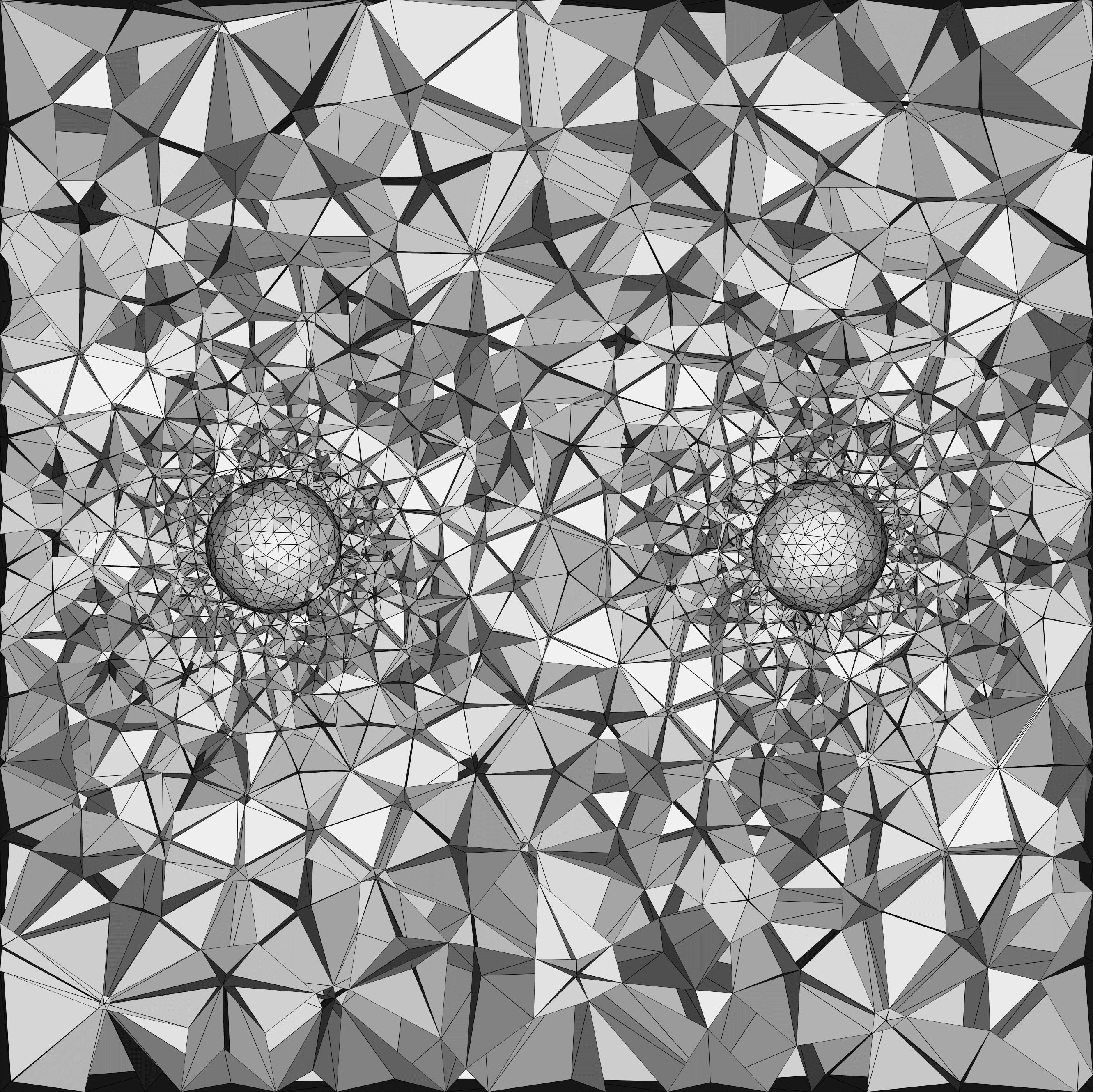
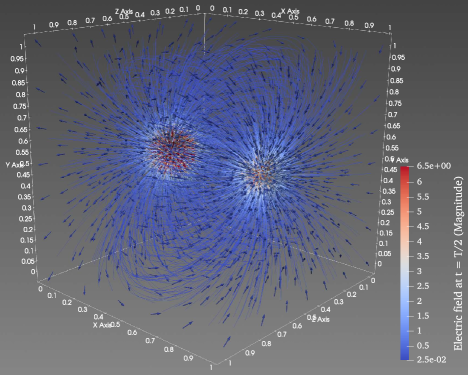
Figure 1: LEFT: intersection of triangulation $\mathcal{T}_{h}$ with ($\mathbb{R}\times\{\frac{1}{2}\}\times\mathbb{R}$)-plane; RIGHT: fully-charged electric field $\boldsymbol{E}(\frac{T}{2})\in C^{\infty}(\overline{\Omega};\mathbb{R}^{3})$ at time $t=\frac{T}{2}$.

As initial condition, we consider a smooth, incompressible vortex flow fulfilling a no-slip boundary condition on $\partial\Omega$. More precisely, the initial velocity vector field $\mathbf{v}_{0}\in H$, for every $x=(x_{1},x_{2},x_{3})^{\top}\in\Omega$, is defined by

$$\mathbf{v}_{0}(x)\coloneqq(-\sin(2\pi x_{2})(1-\cos(2\pi x_{1})),\sin(2\pi x_{1})(1-\cos(2\pi x_{2})),0)^{\top}\,.$$ (9.13)

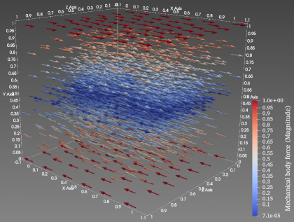
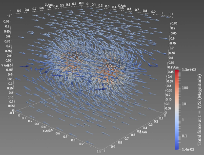
Figure 2: LEFT: mechanical body force $\widehat{\boldsymbol{f}}\in C^{\infty}(\overline{\Omega};\mathbb{R}^{3})$; RIGHT: total force $\boldsymbol{f}(\frac{T}{2})\in C^{\infty}(\overline{\Omega};\mathbb{R}^{3})$ at time $t=\frac{T}{2}$, i.e., when the electric field is fully-charged (in a $\log$-plot).

Since $\hat{p}\in W^{1,\infty}(\mathbb{R}_{\geq 0})$, we have that $p\in W^{1,\infty}(Q_{T})$. In particular, the power-law index ${p\in W^{1,\infty}(Q_{T})}$ is approximated by $p_{h}\in\mathbb{P}^{0}(\mathcal{I}_{h};\mathbb{P}^{0}(\mathcal{T}_{h}))$, $h\in(0,1]$, which is obtained by employing the same one-point quadrature rule from the previous section (i.e., (8.1) with (8.2)). We use the Taylor–Hood element on a triangulation $\mathcal{T}_{h}$ with 4.947 vertices and 26.903 tetrahedra to compute ${(\mathbf{v}_{h}^{k},\pi_{h}^{k})^{\top}\in{\mathaccent 23{V}}_{h,0}\times{\mathaccent 23{Q}}_{h}}$, ${k=1,\ldots,K}$, where $K=128$, solving (9.1). In doing so, due to $\boldsymbol{f}\in W^{1,\infty}(Q_{T};\mathbb{R}^{3})$, again, for every $k=1,\ldots,K$, we replace the $k$-th. temporal mean $\langle\Pi_{h}^{0,\mathrm{x}}\boldsymbol{f}\rangle_{k}\in(\mathbb{P}^{0}(\mathcal{T}_{h}))^{3}$ by the temporal evaluation $\Pi_{h}^{0,\mathrm{x}}\boldsymbol{f}(t_{k})\in(\mathbb{P}^{0}(\mathcal{T}_{h}))^{3}$. To better compare the influence of the charging and discharging of the electric field $\boldsymbol{E}\in W^{1,\infty}(Q_{T};\mathbb{R}^{3})$, we carry out two different numerical test cases:

$\bullet$ Numerical test cases:

(Test Case 1).  In this case, the electric field is never charged, i.e., instead of (9.12), we set ${\boldsymbol{E}\coloneqq\mathbf{0}}$ in $Q_{T}$, so that the total force just becomes the mechanical body force, i.e., $\boldsymbol{f}=\widehat{\boldsymbol{f}}$ in $Q_{T}$ (cf. Figure 2(LEFT)).

(Test Case 2).  In this case, the electric field is defined by (9.12) (i.e., it linearly charges from $t=0$ to $t=\frac{T}{4}$, is fully-charged from $t=\frac{T}{4}$ to $t=\frac{3T}{4}$ (cf. Figure 1(RIGHT)), and linearly discharges from $t=\frac{3T}{4}$ to $t=T$), so that the total forces is given via $\boldsymbol{f}=\widehat{\boldsymbol{f}}+\chi_{E}\textup{div}_{x}(\boldsymbol{E}\otimes\boldsymbol{E})$ in $Q_{T}$ (cf. Figure 2(RIGHT)).

$\bullet$ Observations:

(Test Case 1).  In this case, the magnitudes of the velocity vector field (cf. Figure 5) and the kinematic pressure (cf. Figure 3) slightly reduce as the temporally constant total force $\boldsymbol{f}=\widehat{\boldsymbol{f}}$ (cf. Figure 2(LEFT)) is not sufficient to fully maintain the initial vortex flow $\mathbf{v}_{0}\in H$ (cf. (9.13)).

(Test Case 2).  In this case, at time $t=\frac{T}{2}$, when the electric field $\boldsymbol{E}(\frac{T}{2})\in C^{\infty}(\overline{\Omega};\mathbb{R}^{3})$ is fully-charged (cf. Figure 1(RIGHT)), the total force $\boldsymbol{f}(\frac{T}{2})\in C^{\infty}(\overline{\Omega};\mathbb{R}^{3})$ generates a high attraction close to the two holes (cf. Figure 2(RIGHT)), where the electrodes are located, so that the magnitudes of both velocity vector field and the kinematic pressure significantly increase close to these two holes. To be more precise, the magnitude of velocity vector field is increased by a factor of about $10$ (cf. Figure 6(LEFT)) compared to (Test Case 2) (cf. Figure 5(LEFT)), while the magnitude of the kinematic pressure is increased by a factor of about $10^{5}$ (cf. Figure 4(LEFT)) compared to (Test Case 2) (cf. Figure 3(LEFT)). At time $t=T$, when the electric field is fully-discharged, the total force becomes the mechanical body force enforcing a simple vortex flow, so that the velocity vector field (cf. Figure 6(RIGHT)) and kinematic pressure (cf. Figure 4(RIGHT)) arrive at states similar to (Test Case 1) at time $t=T$ (cf. Figure 5(RIGHT) and Figure 3(RIGHT)). This mimics the rapid change of states possible with electro-rheological fluids.

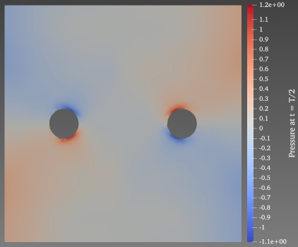
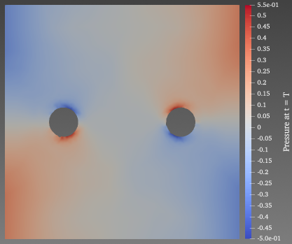
Figure 3: LEFT: discrete kinematic pressure $\pi_{h}^{64}\in\mathbb{P}^{1}_{c}(\mathcal{T}_{h})$ intersected with the ($\mathbb{R}\times\{\frac{1}{2}\}\times\mathbb{R}$)-plane (i.e., at time $t=\frac{T}{2}$) in (Test Case 1); RIGHT: discrete kinematic pressure $\pi_{h}^{128}\in\mathbb{P}^{1}_{c}(\mathcal{T}_{h})$ intersected with the ($\mathbb{R}\times\{\frac{1}{2}\}\times\mathbb{R}$)-plane (i.e., at time $t=T$) in (Test Case 1).

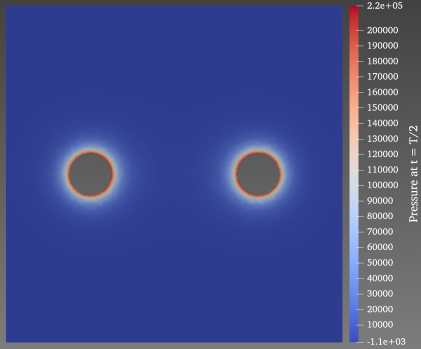
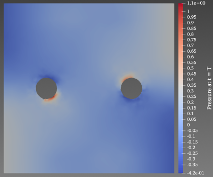
Figure 4: LEFT: discrete kinematic pressure $\pi_{h}^{64}\in\mathbb{P}^{1}_{c}(\mathcal{T}_{h})$ intersected with the ($\mathbb{R}\times\{\frac{1}{2}\}\times\mathbb{R}$)-plane (i.e., at time $t=\frac{T}{2}$) in (Test Case 2); RIGHT: discrete kinematic pressure $\pi_{h}^{128}\in\mathbb{P}^{1}_{c}(\mathcal{T}_{h})$ intersected with the ($\mathbb{R}\times\{\frac{1}{2}\}\times\mathbb{R}$)-plane (i.e., at time $t=T$) in (Test Case 2).

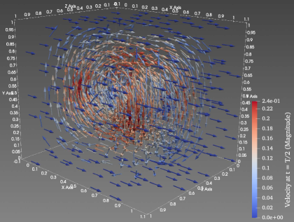
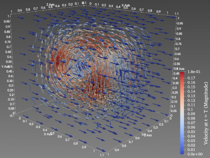
Figure 5: LEFT: discrete velocity vector field $\mathbf{v}_{h}^{64}\in(\mathbb{P}^{2}(\mathcal{T}_{h}))^{3}$ (i.e., at time $t=\frac{T}{2}$) in (Test Case 1); RIGHT: discrete velocity vector field $\mathbf{v}_{h}^{128}\in(\mathbb{P}^{2}(\mathcal{T}_{h}))^{3}$ (i.e., at time $t=T$) in (Test Case 1).

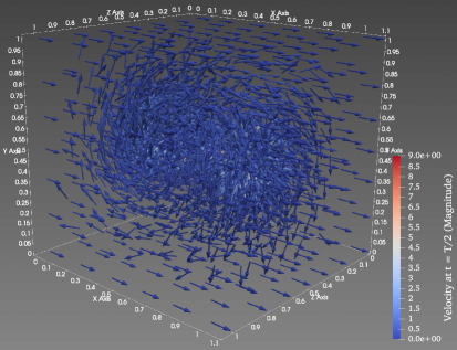
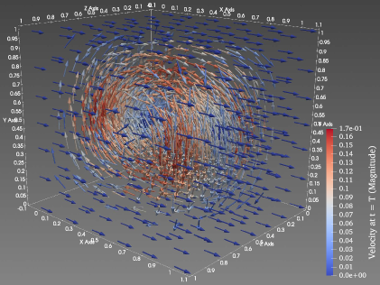
Figure 6: LEFT: discrete velocity vector field $\mathbf{v}_{h}^{64}\in(\mathbb{P}^{2}(\mathcal{T}_{h}))^{3}$ (i.e., at time $t=\frac{T}{2}$) in (Test Case 2); RIGHT: discrete velocity vector field $\mathbf{v}_{h}^{128}\in(\mathbb{P}^{2}(\mathcal{T}_{h}))^{3}$ (i.e., at time $t=T$) in (Test Case 2).

References

- [1] J. Ahrens, B. Geveci, and C. Law, Visualization Handbook, ch. ParaView: An End-User Tool for Large Data Visualization, pp. 717–731, Elsevier Inc., Burlington, MA, USA, 2005. Available at https://www.sciencedirect.com/book/9780123875822/visualization-handbook.
- [2] C. R. Harris et al., Array programming with NumPy, Nature 585 no. 7825 (2020), 357–362. doi:10.1038/s41586-020-2649-2.
- [3] P. R. Amestoy, I. S. Duff, J.-Y. L’Excellent, and J. Koster, A fully asynchronous multifrontal solver using distributed dynamic scheduling, SIAM J. Matrix Anal. Appl. 23 no. 1 (2001), 15–41. doi:10.1137/S0895479899358194.
- [4] S. N. Antontsev and J. F. Rodrigues, On stationary thermo-rheological viscous flows, Ann. Univ. Ferrara Sez. VII Sci. Mat. 52 no. 1 (2006), 19–36. doi:10.1007/s11565-006-0002-9.
- [5] D. N. Arnold, F. Brezzi, and M. Fortin, A stable finite element for the Stokes equations, Calcolo 21 no. 4 (1984), 337–344 (1985). doi:10.1007/BF02576171.
- [6] S. Bartels, Numerical methods for nonlinear partial differential equations, Springer Series in Computational Mathematics 47, Springer, Cham, 2015. doi:10.1007/978-3-319-13797-1.
- [7] A. Behera, Advanced Materials, Springer, Cham, 2021. doi:10.1007/978-3-030-80359-9.
- [8] L. Belenki, L. C. Berselli, L. Diening, and M. Růžička, On the finite element approximation of -Stokes systems, SIAM J. Numer. Anal. 50 no. 2 (2012), 373–397.doi:10.1137/10080436X.
- [9] C. Bernardi and G. Raugel, Analysis of some finite elements for the Stokes problem, Math. Comp. 44 no. 169 (1985), 71–79. doi:10.2307/2007793.
- [10] L. C. Berselli and A. Kaltenbach, Error analysis for a finite element approximation of the steady -Navier-Stokes equations, 2023. arXiv 2311.00534.
- [11] D. Boffi, F. Brezzi, and M. Fortin, Mixed finite element methods and applications, Springer Series in Computational Mathematics 44, Springer, Heidelberg, 2013. doi:10.1007/978-3-642-36519-5.
- [12] D. Breit and P. Mensah, Space-time approximation of parabolic systems with variable growth, IMA Journal of Numerical Analysis 40 no. 4 (2019), 2505–2552. doi:10.1093/imanum/drz039.
- [13] D. Breit and F. Gmeineder, Electro-rheological fluids under random influences: martingale and strong solutions, Stoch. Partial Differ. Equ. Anal. Comput. 7 no. 4 (2019), 699–745. doi:10.1007/s40072-019-00138-6.
- [14] D. Breit and P. R. Mensah, Space-time approximation of parabolic systems with variable growth, IMA J. Numer. Anal. 40 no. 4 (2020), 2505–2552. doi:10.1093/imanum/drz039.
- [15] C. Bridges, S. Karra, and K. R. Rajagopal, On modeling the response of the synovial fluid: unsteady flow of a shear-thinning, chemically-reacting fluid mixture, Comput. Math. Appl. 60 no. 8 (2010), 2333–2349. doi:10.1016/j.camwa.2010.08.027.
- [16] I. A. Brigadnov and A. Dorfmann, Mathematical modeling of magnetorheological fluids, Contin. Mech. Thermodyn. 17 no. 1 (2005), 29–42 (English). doi:10.1007/s00161-004-0185-1.
- [17] M. Bulíček, P. Gwiazda, J. Skrzeczkowski, and J. Woźnicki, Non-Newtonian fluids with discontinuous-in-time stress tensor, J. Funct. Anal. 285 no. 2 (2023), Paper No. 109943, 42. doi:10.1016/j.jfa.2023.109943.
- [18] E. Carelli, J. Haehnle, and A. Prohl, Convergence analysis for incompressible generalized Newtonian fluid flows with nonstandard anisotropic growth conditions, SIAM J. Numer. Anal. 48 no. 1 (2010), 164–190. doi:10.1137/080718978.
- [19] P. Clément, Approximation by finite element functions using local regularization, RAIRO Analyse Numérique 9 no. R-2 (1975), 77–84.
- [20] M. Crouzeix and P.-A. Raviart, Conforming and nonconforming finite element methods for solving the stationary Stokes equations. I, Rev. Française Automat. Informat. Recherche Opérationnelle Sér. Rouge 7 no. no. , no. R-3 (1973), 33–75.
- [21] D. V. Cruz-Uribe and A. Fiorenza, Variable Lebesgue spaces, Birkhäuser/Springer, Heidelberg, 2013, Foundations and harmonic analysis. doi:10.1007/978-3-0348-0548-3.
- [22] L. Diening, Theoretical and numerical results for electrorheological fluids, 2002, PhD thesis, University Freiburg.
- [23] L. Diening, C. Kreuzer, and S. Schwarzacher, Convex hull property and maximum principle for finite element minimisers of general convex functionals, Numer. Math. 124 no. 4 (2013), 685–700. doi:10.1007/s00211-013-0527-7.
- [24] L. Diening, J. Storn, and T. Tscherpel, Fortin operator for the Taylor-Hood element, Numer. Math. 150 no. 2 (2022), 671–689. doi:10.1007/s00211-021-01260-1.
- [25] L. Diening, P. Harjulehto, P. Hästö, and M. Růžička, Lebesgue and Sobolev spaces with variable exponents, Lecture Notes in Mathematics 2017, Springer, Heidelberg, 2011. doi:10.1007/978-3-642-18363-8.
- [26] L. Diening, C. Kreuzer, and E. Süli, Finite element approximation of steady flows of incompressible fluids with implicit power-law-like rheology, SIAM J. Numer. Anal. 51 no. 2 (2013), 984–1015 (English). doi:10.1137/120873133.
- [27] W. Eckart and M. Růžička, Modeling micropolar electrorheological fluids, Int. J. Appl. Mech. Eng. 11 (2006), 813–844.
- [28] A. C. Eringen, Microcontinuum field theories. I. Foundations and solids, Springer-Verlag, New York, 1999. doi:10.1007/978-1-4612-0555-5.
- [29] A. Ern and J.-L. Guermond, Theory and practice of finite elements, Applied Mathematical Sciences 159, Springer-Verlag, New York, 2004. doi:10.1007/978-1-4757-4355-5.
- [30] A. Ern and J. L. Guermond, Finite Elements I: Approximation and Interpolation, Texts in Applied Mathematics no. 1, Springer International Publishing, 2021. doi:10.1007/978-3-030-56341-7.
- [31] H. Gajewski, K. Gröger, and K. Zacharias, Nichtlineare Operatorgleichungen und Operatordifferentialgleichungen, Akademie-Verlag, Berlin, 1974.
- [32] V. Girault and J.-L. Lions, Two-grid finite-element schemes for the transient Navier-Stokes problem, M2AN Math. Model. Numer. Anal. 35 no. 5 (2001), 945–980. doi:10.1051/m2an:2001145.
- [33] V. Girault and P.-A. Raviart, Finite element methods for Navier-Stokes equations, Springer Series in Computational Mathematics 5, Springer-Verlag, Berlin, 1986, Theory and algorithms.doi:10.1007/978-3-642-61623-5.
- [34] V. Girault and L. R. Scott, A quasi-local interpolation operator preserving the discrete divergence, Calcolo 40 no. 1 (2003), 1–19. doi:10.1007/s100920300000.
- [35] J. D. Hunter, Matplotlib: A 2d graphics environment, Computing in Science & Engineering 9 no. 3 (2007), 90–95. doi:10.1109/MCSE.2007.55.
- [36] T. M. Inc., Matlab version: 9.13.0 (r2022b), 2022. Available at https://www.mathworks.com.
- [37] A. Kaltenbach, Theory of Pseudo-Monotone Operators for Unsteady Problems in Variable Exponent Spaces, dissertation, Institute of Applied Mathematics, University of Freiburg, 2021, p. 235. doi:10.6094/UNIFR/222538.
- [38] A. Kaltenbach and M. Růžička, Note on the existence theory for pseudo-monotone evolution problems, J. Evol. Equ. 21 no. 1 (2021), 247–276. doi:10.1007/s00028-020-00577-y.
- [39] A. Kaltenbach, Pseudo-Monotone Operator Theory for Unsteady Problems with Variable Exponents, Lecture Notes in Mathematics 2329, Springer, Cham, 2023. doi:10.1007/978-3-031-29670-3.
- [40] S. Ko, P. Pustějovská, and E. Süli, Finite element approximation of an incompressible chemically reacting non-Newtonian fluid, ESAIM Math. Model. Numer. Anal. 52 no. 2 (2018), 509–541. doi:10.1051/m2an/2017043.
- [41] W. M. Lai, S. C. Kuei, and V. C. Mow, Rheological Equations for Synovial Fluids, Journal of Biomechanical Engineering 100 no. 4 (1978), 169–186. doi:10.1115/1.3426208.
- [42] R. Landes and V. Mustonen, A strongly nonlinear parabolic initial-boundary value problem, Ark. Mat. 25 no. 1 (1987), 29–40. doi:10.1007/BF02384435.
- [43] A. Logg and G. N. Wells, Dolfin: Automated finite element computing, ACM Transactions on Mathematical Software 37 no. 2 (2010), 1–28. doi:10.1145/1731022.1731030.
- [44] M. t. Musy, marcomusy/vedo: 2023.4.4, 3. doi:10.5281/zenodo.7734756
- [45] S. E. Pastukhova, Compensated compactness principle and solvability of generalized Navier-Stokes equations, 173, 2011, Problems in mathematical analysis. No. 55, pp. 769–802. doi:10.1007/s10958-011-0271-4.
- [46] P.-O. Persson and G. Strang, A Simple Mesh Generator in MATLAB, SIAM Review 46 no. 2 (2004), 329–345. doi:10.1137/S0036144503429121.
- [47] K. Rajagopal and M. Růžička, On the modeling of electrorheological materials, Mechanics Research Communications 23 no. 4 (1996), 401–407. doi:https://doi.org/10.1016/0093-6413(96)00038-9.
- [48] T. Roubíček, Nonlinear partial differential equations with applications, second ed., International Series of Numerical Mathematics 153, Birkhäuser/Springer Basel AG, Basel, 2013. doi:10.1007/978-3-0348-0513-1.
- [49] M. Růžička, Electrorheological Fluids: Modeling and Mathematical Theory, Lecture Notes in Math. 1748, Springer, Berlin, 2000. doi:https://doi.org/10.1007/BFb0104029.
- [50] J. Svensson, mat4py, 8 2014. Available at https://github.com/nephics/mat4py/tree/master.
- [51] C. Taylor and P. Hood, A numerical solution of the Navier-Stokes equations using the finite element technique, Internat. J. Comput. & Fluids 1 no. 1 (1973), 73–100. doi:10.1016/0045-7930(73)90027-3.
- [52] R. Temam, Navier-Stokes equations, AMS Chelsea Publishing, Providence, RI, 2001, Theory and numerical analysis, Reprint of the 1984 edition.doi:10.1090/chel/343.
- [53] E. Zeidler, Nonlinear functional analysis and its applications. II/B, Springer, New York, 1990, Nonlinear monotone operators.
- [54] X. Zhang and Q. Sun, Characterizations of variable fractional Hajłasz–Sobolev spaces, 2022. arXiv 2204.11612
- [55] V. V. Zhikov, Meyer-type estimates for solving the nonlinear Stokes system, Differ. Uravn. 33 no. 1 (1997), 107–114, 143.
- [56] V. V. Zhikov, On the solvability of the generalized Navier-Stokes equations, Dokl. Akad. Nauk 423 no. 5 (2008), 597–602. doi:10.1134/S1064562408060240.