Sparse Autoregressive Neural Networks for Classical Spin Systems

Abstract

Efficient sampling and approximation of Boltzmann distributions involving large sets of binary variables, or spins, are pivotal in diverse scientific fields even beyond physics. Recent advancements in generative neural networks have significantly impacted this domain. However, those neural networks are often treated as black boxes, with architectures primarily influenced by data-driven problems in computational science. Addressing this gap, we introduce a novel autoregressive neural network architecture named TwoBo, specifically designed for sparse two-body interacting spin systems. We directly incorporate the Boltzmann distribution into its architecture and parameters, resulting in enhanced convergence speed, superior free energy accuracy, and reduced trainable parameters. We perform numerical experiments on disordered, frustrated systems with more than $1000$ spins on grids and random graphs, and demonstrated its advantages compared to previous autoregressive and recurrent architectures. Our findings validate a physically informed approach and suggest potential extensions to multi-valued variables and many-body interaction systems, paving the way for broader applications in scientific research.

Introduction

This paper addresses the challenge of efficiently sampling and approximating the Boltzmann distribution in systems characterized by two-body interacting binary variables, or spins. The interactions among the variables are typically defined on sparse graphs, such as lattice systems pivotal in material science, and random graphs that model a plethora of complex socio-technological systems [Barabási and Albert, 1999, Albert and Barabási, 2002]. The complexity of the system’s Boltzmann distribution, and thus its underlying physics, significantly depends on the couplings and external field values. For instance, disordered or random coupling values lead to complex and frustrated systems that could reduce the efficiency of sampling algorithms like Monte Carlo approaches. This complexity finds relevance in diverse areas, including spin glasses [Mezard et al., 1986], optimization on random graphs [Mezard and Montanari, 2009], and statistical inference problems [Zdeborová and Krzakala, 2016].

Accurate approximation and efficient sampling of the Boltzmann distribution is crucial for solving problems in various fields, ranging from biology [Cocco et al., 2018] to computer science [Mézard et al., 2002]. The recent advent of deep generative models, particularly autoregressive neural networks (ARNNs), has marked a significant advancement in fields like image and language generation [Brown et al., 2020]. A pivotal study in 2019 introduced the use of ARNNs for Boltzmann distribution sampling [Wu et al., 2019], leading to a proliferation of research in both classical [Nicoli et al., 2020, McNaughton et al., 2020, Pan et al., 2021, Wu et al., 2021, Hibat-Allah et al., 2021a] and quantum physics [Sharir et al., 2020, Luo et al., 2022, Wang and Davis, 2020, Hibat-Allah et al., 2020, Liu et al., 2021, Barrett et al., 2022, Cha et al., 2021, Wu et al., 2023], as well as in statistical inference [Biazzo et al., 2022] and optimization problems [Khandoker et al., 2023].

The ARNN architectures used are typically adapted from those developed for data-driven problems in computer science, and prior knowledge on theoretical properties of the physical system has rarely been utilized to customize the ARNN architecture, or only been exploited for specific physical systems [Białas et al., 2022, Biazzo et al., 2022]. Recently, it was established a direct mapping between the Boltzmann distribution and the corresponding ARNN architecture [Biazzo, 2023]. The derived general architecture was not directly usable, but thanks to the analytic derivation, two specific architectures for two well-known fully connected spin models, the Curie–Weiss model and the Sherringhton–Kirkpatrick model, were derived.

The contribution of this work is a novel ARNN architecture tailored for general two-body interacting systems, which exploits the knowledge of the Hamiltonian and the Boltzmann distribution. The proposed architecture has a part of its parameters precomputed from the Hamiltonian couplings and takes advantage of the usual sparsity of the interactions among spins. It has fewer trainable parameters and a faster convergence speed than conventional ARNN architectures while maintaining a high expressivity. This universal method can be applied across two-body interacting systems, offering a more efficient sampling approach than standard ARNN architectures and opening the way to richer, physically informed neural network architectures.

Methods

Consider a system of $N$ spins characterized by a Hamiltonian $H$. These spins, each denoted as $\sigma_{i}$, can take values in $\pm 1$. Let $\bm{\sigma}=\{\sigma_{1},\sigma_{2},\ldots,\sigma_{N}\}$ represent the set of all spins. The Hamiltonian is given by $H(\bm{\sigma})=-\sum_{\langle i,j\rangle}J_{ij}\sigma_{i}\sigma_{j}-\sum_{i}h_{i}\sigma_{i}$, where the summation $\sum_{\langle i,j\rangle}$ extends over all interacting pairs of spins. The term $J_{ij}$ represents the interaction strengths between the spins, and $h_{i}$ is the external magnetic field acting on each spin.

We approximate the Boltzmann distribution $P(\bm{\sigma})$ employing an ARNN whose probability distribution is decomposed in the autoregressive form $Q(\bm{\sigma})=\prod_{i}Q_{i}(\sigma_{i}\mid\bm{\sigma}_{<i})$, where $\bm{\sigma}_{<i}=\{\sigma_{1},\sigma_{2},\ldots,\sigma_{i-1}\}$ denotes the set of variables with indices less than $i$. If we can write a probability distribution in this form, then the ancestral sampling procedure, where each variable $\sigma_{i}$ is sampled in the subsequent order according to its conditional probability $Q_{i}(\sigma_{i}\mid\bm{\sigma}_{<i})$ given the previous variables, produces guaranteed independent samples.

We parameterize each conditional probability with a neural network. Without limitation to particular interacting systems, variable sharing schemes, or recurrent structures, one may use feed-forward neural networks to parametrize the conditional probabilities, with masked dense layers to assure the autoregressive property. This architecture is known as masked autoencoder for distribution estimation (MADE), which was first introduced in [Germain et al., 2015] and used in physics in [Wu et al., 2019]. However, its number of parameters and the computation time of each layer both scale by $O(N^{2})$ with the system size $N$, limiting its applicability to small systems.

In the following, we will show how the knowledge of the Hamiltonian and the Boltzmann distribution leads to systematically reducing both the number of trainable parameters and the computation time. Consider the Boltzmann distribution $P_{\text{B}}(\bm{\sigma})=\frac{\rme^{-\beta H(\bm{\sigma})}}{Z}$, where $\beta$ is the inverse temperature and $Z=\sum_{\bm{\sigma}}\rme^{-\beta H(\bm{\sigma})}$ is the normalization factor. Following the derivation presented in [Biazzo, 2023], we can write:

$$P_{\text{B}i}(\sigma_{i}\mid\bm{\sigma}_{<i})=\frac{\sum_{\bm{\sigma}_{>i}}P_{\text{B}}(\bm{\sigma})}{\sum_{\bm{\sigma}_{>i-1}}P_{\text{B}}(\bm{\sigma})}=\frac{\sum_{\bm{\sigma}_{>i}}\rme^{-\beta H(\bm{\sigma})}}{\sum_{\bm{\sigma}_{>i-1}}\rme^{-\beta H(\bm{\sigma})}}=\frac{f(\sigma_{i},\bm{\sigma}_{<i})}{\sum_{\sigma_{i}}f(\sigma_{i},\bm{\sigma}_{<i})},$$ (1)

where we defined $f(\sigma_{i},\bm{\sigma}_{<i})=\sum_{\bm{\sigma}_{>i}}\rme^{-\beta H(\bm{\sigma})}$. The positive conditional probability of variable $\sigma_{i}$ can be written as:

$$P_{\text{B}i}(\sigma_{i}=+1\mid\bm{\sigma}_{<i})=\frac{f(\sigma_{i}=+1,\bm{\sigma}_{<i})}{f(\sigma_{i}=+1,\bm{\sigma}_{<i})+f(\sigma_{i}=-1,\bm{\sigma}_{<i})}=S\left(\log\frac{f(\sigma_{i}=+1,\bm{\sigma}_{<i})}{f(\sigma_{i}=-1,\bm{\sigma}_{<i})}\right),$$ (2)

where we impose the sigmoid function $S(x)=\frac{1}{1+\rme^{-x}}$ as the last layer of the neural network. This ensures that the network’s output is constrained to lie between zero and one. Substituting the definition of the Hamiltonian and the Boltzmann distribution, we obtain:

$$P_{\text{B}i}(\sigma_{i}=+1\mid\bm{\sigma}_{<i})=S\left(2\beta\sum_{s<i}J_{si}\sigma_{s}+2\beta h_{i}+\log\frac{\rho_{i}^{+}(\bm{\sigma}_{<i})}{\rho_{i}^{-}(\bm{\sigma}_{<i})}\right),$$ (3)

where:

$$\rho_{i}^{\pm}(\bm{\sigma}_{<i})=\sum_{\bm{\sigma}_{>i}}\exp\beta\left(\sum_{l>i}\sigma_{l}\left(\pm J_{il}+\sum_{s<i}J_{sl}\sigma_{s}+h_{l}\right)+\sum_{l,l^{\prime}>i}J_{ll^{\prime}}\sigma_{l}\sigma_{l^{\prime}}\right).$$ (4)

Observing $\rho_{i}^{\pm}$ as a sequence of operations on the input variables $\bm{\sigma}_{<i}$, the first operation is a linear transformation, which leads us to define a linear layer with the outputs:

$$\xi_{il}=\sum_{s<i}J_{sl}\sigma_{s}\quad\text{with}\quad l\geq i.$$ (5)

Now Eq. (3) can be written as:

$$P_{\text{B}i}(\sigma_{i}=+1\mid\bm{\sigma}_{<i})=S\left(2\beta\xi_{ii}+2\beta h_{i}+\rho_{i}(\bm{\xi}_{i})\right),$$ (6)

where we defined $\rho_{i}(\bm{\xi}_{i})=\log\frac{\rho_{i}^{+}(\bm{\xi}_{i})}{\rho_{i}^{-}(\bm{\xi}_{i})}$ and $\bm{\xi}_{i}=\{\xi_{i,i+1},\xi_{i,i+2},\ldots,\xi_{i,N}\}$. The variables $\bm{\xi}_{i}$ can be explicitly computed given the input spins $\bm{\sigma}_{<i}$ and the Hamiltonian parameters $\bm{J}$, which means that the first layer of our neural network does not involve any trainable parameter. After the first layer, the term $2\beta\xi_{ii}$ appears as an input to the last layer $S$, which can be considered as a skip connection [He et al., 2016]. As shown in Eq. (4), the exact computation of the function $\rho_{i}$ involves a sum over all configurations of $\bm{\sigma}_{>i}$, which scales exponentially with the system size. The whole network architecture to compute Eq. (6) is sketched in Fig. 1 (a).

In [Biazzo, 2023], the functions $\rho_{i}$ were approximated with specific architectures derived for the fully connected Curie–Weiss and Sherrington–Kirkpatrick models. In the present work, we propose a more general approach to approximate $\rho_{i}$ using feed-forward neural networks, whose inputs are the variables $\bm{\xi}_{i}$, and to take advantage of the sparsity of interactions among the spins. In the following, we refer to this architecture as TwoBo (two-body interactions).

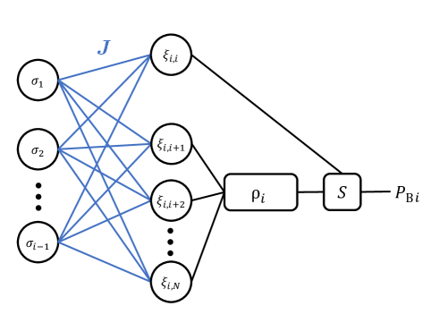
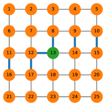
Figure 1: (a) Sketch of the TwoBo neural network architecture to compute a conditional probability $P_{\text{B}i}(\sigma_{i}=+1\mid\bm{\sigma}_{<i})$ in the autoregressively decomposed Boltzmann distribution. The parameters of the first layer are taken from the coupling matrix $\bm{J}$. The function $\rho_{i}$ is parameterized as a feed-forward neural network, whose inputs are the variables $\bm{\xi}_{i}$ after the first layer. The last layer $S$ is a sigmoid function. (b) Computing the conditional probability $P_{\text{B}i}$ with $i=13$ on a 2D grid of $N=25$. The edges between the spins $\bm{\sigma}_{<i}$ and $\bm{\sigma}_{\geq i}$ are highlighted in blue, and only those edges are used when computing $\xi_{il}$. Among the variables $\{\xi_{il}\mid l>i\}$, only those with $l<i+L$ are kept as inputs to $\rho_{i}$, and the others are ensured to be zero.

When computing a conditional probability $P_{\text{B}i}$ with a fixed $i$, the computation time of the first layer, Eq. (5), scales linearly in the number of non-zero elements in $\bm{J}$. For fully connected interactions it scales as $O(N^{2})$ with the system size $N$, whereas for sparse interactions it is linear in $N$. Moreover, in the case of sparse interactions, lots of the variables in $\bm{\xi}_{i}$ are ensured to be zero. As seen from Eq. (5), if the spin $\sigma_{l}$ does not interact with all the spins $\bm{\sigma}_{<i}$, then $\xi_{il}$ is zero and can be discarded in the parametrization of the function $\rho_{i}$. Consider for instance a 2D grid of side length $L$, with spins $\bm{\sigma}$ ordered as in Fig. 1 (b). The variables $\xi_{il}$ are non-zero only when $i<l<i+L$, so the number of variables in $\bm{\xi}_{i}$ is reduced from $O(N)=O(L^{2})$ to $O(L)$. Furthermore, as the Hamiltonian is locally interacting, each remaining $\xi_{il}$ only depends on a fixed number of spins, which does not scale with $N$, so the computation time of the first layer is only $O(L)$. When we compute all conditional probabilities $\{P_{\text{B}i}\mid 1\leq i\leq N\}$ in a batch, the computation time of the first layer is $O(LN)=O(L^{3})$, which is polynomially lower than $O(L^{4})$ of MADE. After the first layer, we use a lightweight neural network for $\rho_{i}$, whose computational complexity does not exceed $O(L^{3})$. Empirical scaling of the number of trainable parameters is shown in the Supplementary Material A.

When training the neural network in a variational setting, we denote it as $Q^{\theta}(\bm{\sigma})$, where $\theta$ is the set of trainable parameters. The parameters are trained to minimize the Kullback–Leibler divergence $D_{\text{KL}}(Q^{\theta}\mid\mid P)=\sum_{\bm{\sigma}}Q^{\theta}(\bm{\sigma})\log\frac{Q^{\theta}(\bm{\sigma})}{P(\bm{\sigma})}$ between the variational and the target distributions. When the target is the Boltzmann distribution $P_{\text{B}}$, it is equivalent to minimizing the variational free energy $F^{\theta}=\sum_{\bm{\sigma}}Q^{\theta}(\bm{\sigma})\left(\frac{1}{\beta}\log Q^{\theta}(\bm{\sigma})+H(\bm{\sigma})\right)$, apart from a constant term. Its exact computation involves a summation over the spin configurations that grows exponentially with the system size. In [Wu et al., 2019], it was proposed to estimate the variational free energy and its gradients with respect to $\theta$ by a finite subset of configurations sampled from the ARNN thanks to the ancestral sampling procedure.

In this work, to alleviate the problem of mode collapse, an annealing procedure is used in the training, starting from a low value of $\beta=0.05$ (high temperature) and changing it in steps of $0.05$ until $\beta=3$. In each temperature step, a fixed number of optimization steps are executed, then the trained neural network is used as the initialization in the next temperature. In the case of TwoBo, the $\beta$ used in the skip connection coefficient in Eq. (6) is also updated accordingly, and its effect is shown in the Supplementary Material B.

Results

We test the performance of TwoBo in approximating the Boltzmann distribution of sparse and disordered interacting spin systems, using Edward–Anderson (EA) models of spin glass on 2D and 3D grids with periodic boundary conditions, and random regular graphs (RRG) with fixed degree $d=3$. The couplings $J_{ij}$ are randomly sampled to be either $+1$ or $-1$, and the external fields $h_{i}$ are set to zero for simplicity. Each result we report in this paper is averaged from $10$ random instances, and for each instance we train a neural network respectively.

Although in general we can use a deep feed-forward neural network to parameterize each function $\rho_{i}$ in Eq. (6), in this work we found that a single dense layer is enough to obtain satisfactory results. This dense layer maps $N_{\xi i}$ inputs to one output, where $N_{\xi i}$ is the number of nonzero variables in $\bm{\xi}_{i}$. Note that we do not share the parameters among functions $\rho_{i}$ with different $i$. For comparison, we have tested the simplest MADE with also a single dense layer, which still has more trainable parameters than the simplest TwoBo. Another architecture we have compared to is the tensorized RNN introduced in [Hibat-Allah et al., 2021b] for 2D classical spin systems, where we use $4$ memory units for a comparable number of trainable parameters, and a comparison with RNN at different sizes is shown in the Supplementary Material C. Details of the numerical experiments can be found in the Supplementary Material D.

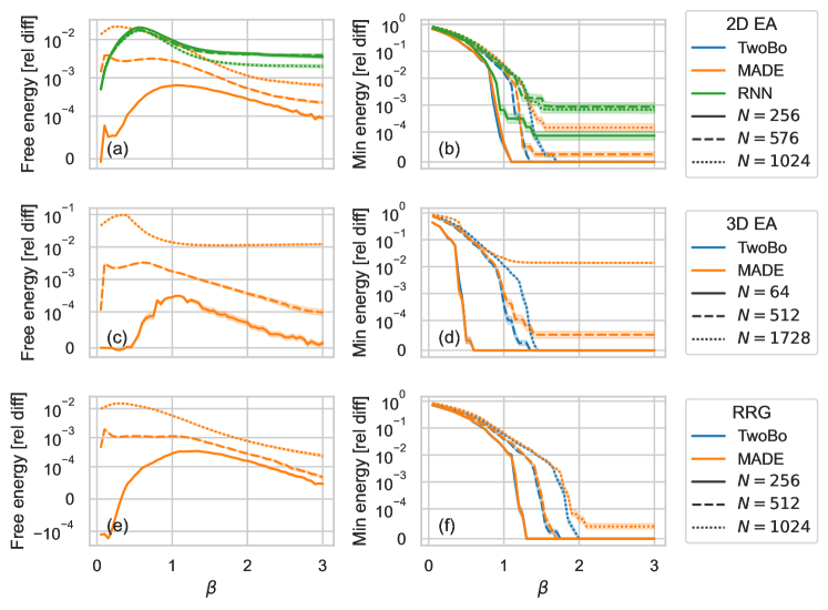
Figure 2: Variational free energy (left column) and minimum energy of sampled configurations (right column) at each $\beta$ on 2D EA (top row), 3D EA (middle row), and RRG (bottom row) models of different sizes. We compare the performances of TwoBo, MADE, and RNN (only in 2D). The variational free energy is shown as the relative difference from TwoBo at the same $\beta$, and the minimum energy as the relative difference from the one found by TwoBo at $\beta=3$. The results are averaged over $10$ random instances of the Hamiltonian, and the error bars show the standard errors over the instances.

In the left column of Fig. 2, the free energies estimated by the three architectures are shown in function of $\beta$, where the TwoBo result is taken as the reference for the relative difference. We observe that TwoBo obtains the lowest free energy estimation on all three interaction graphs, signifying a better approximation of the corresponding Boltzmann distribution.

Recent studies [Ciarella et al., 2023, Inack et al., 2022] have indicated the potential issue of mode collapse that could distort the free energy estimation in highly frustrated systems, where the variational distribution is trapped in local minima of free energy. To corroborate the efficacy of TwoBo in capturing the high complexity of these systems, we have examined its ability to find the ground state configurations, as shown in the right column of Fig. 2. MADE and RNN failed to find configurations with lower energy than TwoBo on large systems, indicating the difficulty in capturing the complexity of these probability distributions.

Besides variational methods, we have used McGroundstate [Charfreitag et al., 2022], a recent max-cut solver for 2D and 3D lattices, to solve the EA instances and compared the results with TwoBo. McGroundstate solved all 2D instances with $N=256,576,1024$ and 3D instances with $N=64$ in provable optimality, as found by TwoBo, but it failed to provide results for larger 3D cases with $N\geq 512$. For the largest 3D cases, we have tried the traditional max-cut algorithm [Burer et al., 2002] implemented in MQLib [Dunning et al., 2018], which yielded energies higher than those obtained by TwoBo. Consequently, we chose the energy found by TwoBo as the reference for the relative difference in minimum energy shown in the right column of Fig. 2.

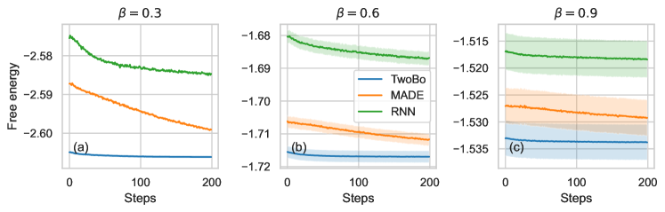
Figure 3: Convergence of variational free energy when training at fixed values of $\beta$ on 2D EA model with $N=576$. The results are averaged over $10$ random instances of the Hamiltonian, and the error bars show the standard errors over the instances.

To investigate the convergence of the training procedure, Fig. 3 shows the free energy during the optimization steps at three different temperatures on a 2D EA model, from which we can observe that TwoBo always starts from a lower free energy compared to the other architectures. This advantage may stem from the fact that the first layer’s parameters are fixed to the Hamiltonian couplings, as well as the change of the skip connection coefficient with $\beta$, leading the variational distribution to be closer to the target distribution at the beginning of the training procedure. With significantly more optimization steps, MADE could eventually match the free energy obtained by TwoBo. In contrast, RNN converges to a higher free energy, indicating its insufficient expressiveness or trainability in the regime of few trainable parameters.

To better assess this claim, Fig. 4 displays the free energy as a function of the number of optimization steps in a whole temperature step. It is evident that as the number of steps increases, the free energy computed by TwoBo systematically decreases. MADE and RNN display a similar trend with almost an order of magnitude more steps, while RNN eventually reaches a plateau with a free energy higher than TwoBo. This comparison shows the abundant expressivity of TwoBo in capturing the target distribution and its ease of training.

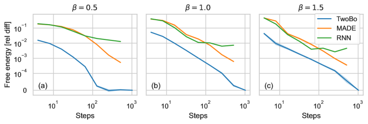
Figure 4: Variational free energy using different numbers of optimization steps at each $\beta$ on 2D EA model with $N=576$, shown as the relative difference from TwoBo at the same $\beta$ using 1024 steps. The results are averaged over $10$ random instances of the Hamiltonian, and the standard errors over the instances are too small to be visible.

Conclusion

In this work, we presented a new autoregressive neural network architecture named TwoBo to sample and approximate the Boltzmann distribution of two-body interacting spin systems. It exploits the knowledge of the target Boltzmann distribution to determine part of its parameters, and systematically reduces the number of trainable parameters in sparse interacting systems without affecting the expressivity. It obtains higher accuracy in approximating disordered and frustrated Boltzmann distributions with considerably fewer trainable parameters and faster convergence than previous ARNN architectures. While the present work focuses on two-body interacting binary variables, nothing prevents using a similar approach for deriving ARNN architectures for multi-valued variables, like Potts models, and with more than two-body interactions.

Data availability statement

The code to reproduce the results and figures presented is openly available at the following URL: https://github.com/cqsl/sparse-twobody-arnn.

References

Supplementary Material

A Scaling of number of trainable parameters

As shown in Fig. S1, on 2D and 3D EA models, the number of trainable parameters in TwoBo scales polynomially slower than that in MADE. On RRG model without a regular grid geometry, TwoBo has the same scaling as MADE, and it only needs half as many parameters.

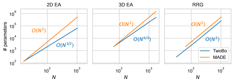
Figure S1: Number of trainable parameters in TwoBo and MADE on 2D EA, 3D EA, and RRG models of various system sizes $N$. For RRG, the number of trainable parameters in TwoBo is averaged over $10$ random instances.

B Annealing $\beta$ in the skip connection coefficient

When optimizing the TwoBo architecture, we not only gradually change the $\beta$ used to compute the variational free energy, but also change the $\beta$ in the skip connection coefficient in Eq. (6) to the same value at each annealing step. If we do not update the $\beta$ in the skip connection coefficient, but fix it to $1$, the resulting variational free energy will be higher especially at the beginning of the annealing procedure, as shown in Fig. S2.

Figure S2: Variational free energy when fixing $\beta=1$ in the skip connection coefficient, shown as the relative difference from updating it during the annealing procedure, on 2D EA model with $N=576$. The results are averaged over $10$ random instances of the Hamiltonian, and the error bars show the standard errors over the instances.

C Comparison with RNN at different sizes

Fig. S3 shows that TwoBo gives lower free energy than RNN with a comparable number of trainable parameters, and the RNN results do not qualitatively change even if we increase the number of trainable parameters by orders of magnitude. When separately examining the estimations of the energy and the entropy, we can see that the high free energy of RNN is mainly because of the entropy is low, which indicates that it is more impacted by mode collapse compared to TwoBo.

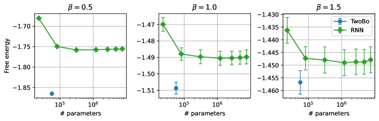
Figure S3: Variational free energy of TwoBo compared to RNN with different numbers of memory units ($2,4,8,16,24,32,40$), on 2D EA model with $N=576$. The results are averaged over $10$ random instances of the Hamiltonian, and the error bars show the standard errors over the instances.

D Details of numerical experiments

In TwoBo and MADE, the only dense layer is initialized using Lecun normal initialization (the default to initialize dense layers in JAX) multiplied by a small factor of $0.01$, so that the output values before the last sigmoid function are small, and after the sigmoid function the probability distribution is almost uniform at the beginning of training, which helps alleviate mode collapse.

The implementation of tensorized RNN is taken from https://github.com/mhibatallah/RNNWavefunctions. We only used their neural network architecture but not their annealing procedure in training, because our annealing procedure aims to produce a converged free energy at each step of $\beta$, while theirs only aims to produce a ground state energy at zero temperature.

At the beginning of training, we run $500$ optimization steps as warm-up with the initial $\beta=0.05$. Then for each $\beta$ in steps of $0.05$ until $\beta=3$, we run $200$ optimization steps. Note that the value of $\beta$ is unchanged during those optimization steps. After each step of $\beta$, the trained neural network is used as the initialization in the next $\beta$. The optimizer we use is Adam [Kingma and Ba, 2015] with learning rate $10^{-3}$, and at each step we take batch size $1024$.

The max-cut solver McGroundstate provides public access through their website. They put a time limit of $1800$ seconds for each spin glass instance, and they failed to solve the 3D EA models with $N=512$ and $1728$ within the time limit. We have run MQLib on our local machine with a time limit of $24$ hours. It outputs the energy whenever it finds a lower one, and it stopped improving the energy after the first hour.

References

- [Albert and Barabási, 2002] Albert, R. and Barabási, A.-L. (2002). Statistical mechanics of complex networks. Rev. Mod. Phys., 74(1):47–97.
- [Barabási and Albert, 1999] Barabási, A.-L. and Albert, R. (1999). Emergence of scaling in random networks. Science, 286(5439):509–512.
- [Barrett et al., 2022] Barrett, T. D., Malyshev, A., and Lvovsky, A. I. (2022). Autoregressive neural-network wavefunctions for ab initio quantum chemistry. Nature Machine Intelligence, 4(4):351–358.
- [Białas et al., 2022] Białas, P., Korcyl, P., and Stebel, T. (2022). Hierarchical autoregressive neural networks for statistical systems. Computer Physics Communications, 281:108502.
- [Biazzo, 2023] Biazzo, I. (2023). The autoregressive neural network architecture of the Boltzmann distribution of pairwise interacting spins systems. Communications Physics, 6(1):296.
- [Biazzo et al., 2022] Biazzo, I., Braunstein, A., Dall’Asta, L., and Mazza, F. (2022). A bayesian generative neural network framework for epidemic inference problems. Scientific Reports, 12(1):19673.
- [Brown et al., 2020] Brown, T., Mann, B., Ryder, N., Subbiah, M., Kaplan, J. D., Dhariwal, P., Neelakantan, A., Shyam, P., Sastry, G., Askell, A., Agarwal, S., Herbert-Voss, A., Krueger, G., Henighan, T., Child, R., Ramesh, A., Ziegler, D., Wu, J., Winter, C., Hesse, C., Chen, M., Sigler, E., Litwin, M., Gray, S., Chess, B., Clark, J., Berner, C., McCandlish, S., Radford, A., Sutskever, I., and Amodei, D. (2020). Language models are few-shot learners. In Advances in Neural Information Processing Systems, volume 33, pages 1877–1901. Curran Associates, Inc.
- [Burer et al., 2002] Burer, S., Monteiro, R. D. C., and Zhang, Y. (2002). Rank-two relaxation heuristics for MAX-CUT and other binary quadratic programs. SIAM J. Optim., 12(2):503–521.
- [Cha et al., 2021] Cha, P., Ginsparg, P., Wu, F., Carrasquilla, J., McMahon, P. L., and Kim, E.-A. (2021). Attention-based quantum tomography. Machine Learning: Science and Technology, 3(1):01LT01.
- [Charfreitag et al., 2022] Charfreitag, J., Jünger, M., Mallach, S., and Mutzel, P. (2022). McSparse: Exact solutions of sparse maximum cut and sparse unconstrained binary quadratic optimization problems. In 2022 Proceedings of the Symposium on Algorithm Engineering and Experiments (ALENEX), pages 54–66.
- [Ciarella et al., 2023] Ciarella, S., Trinquier, J., Weigt, M., and Zamponi, F. (2023). Machine-learning-assisted Monte Carlo fails at sampling computationally hard problems. Machine Learning: Science and Technology, 4(1):010501.
- [Cocco et al., 2018] Cocco, S., Feinauer, C., Figliuzzi, M., Monasson, R., and Weigt, M. (2018). Inverse statistical physics of protein sequences: A key issues review. Reports on Progress in Physics, 81(3):032601.
- [Dunning et al., 2018] Dunning, I., Gupta, S., and Silberholz, J. (2018). What works best when? a systematic evaluation of heuristics for Max-Cut and QUBO. INFORMS Journal on Computing, 30(3).
- [Germain et al., 2015] Germain, M., Gregor, K., Murray, I., and Larochelle, H. (2015). MADE: Masked autoencoder for distribution estimation. In Proceedings of the 32nd International Conference on Machine Learning, volume 37, pages 881–889, Lille, France. PMLR.
- [He et al., 2016] He, K., Zhang, X., Ren, S., and Sun, J. (2016). Deep residual learning for image recognition. In Proceedings of the IEEE Conference on Computer Vision and Pattern Recognition (CVPR).
- [Hibat-Allah et al., 2020] Hibat-Allah, M., Ganahl, M., Hayward, L. E., Melko, R. G., and Carrasquilla, J. (2020). Recurrent neural network wave functions. Phys. Rev. Res., 2(2):023358.
- [Hibat-Allah et al., 2021a] Hibat-Allah, M., Inack, E. M., Wiersema, R., Melko, R. G., and Carrasquilla, J. (2021a). Variational neural annealing. Nature Machine Intelligence, 3(11):1–10.
- [Hibat-Allah et al., 2021b] Hibat-Allah, M., Inack, E. M., Wiersema, R., Melko, R. G., and Carrasquilla, J. (2021b). Variational neural annealing. Nature Machine Intelligence, 3(11):952–961.
- [Inack et al., 2022] Inack, E. M., Morawetz, S., and Melko, R. G. (2022). Neural annealing and visualization of autoregressive neural networks in the newman-moore model. Condensed Matter, 7(2).
- [Khandoker et al., 2023] Khandoker, S. A., Abedin, J. M., and Hibat-Allah, M. (2023). Supplementing recurrent neural networks with annealing to solve combinatorial optimization problems. Machine Learning: Science and Technology, 4(1):015026.
- [Kingma and Ba, 2015] Kingma, D. P. and Ba, J. (2015). Adam: A method for stochastic optimization. In 3rd International Conference on Learning Representations.
- [Liu et al., 2021] Liu, J.-G., Mao, L., Zhang, P., and Wang, L. (2021). Solving quantum statistical mechanics with variational autoregressive networks and quantum circuits. Machine Learning: Science and Technology, 2(2):025011.
- [Luo et al., 2022] Luo, D., Chen, Z., Carrasquilla, J., and Clark, B. K. (2022). Autoregressive neural network for simulating open quantum systems via a probabilistic formulation. Phys. Rev. Lett., 128(9):090501.
- [McNaughton et al., 2020] McNaughton, B., Miloıfmmode \checks\else š\fieviıfmmode \acutec\else ć\fi, M. V., Perali, A., and Pilati, S. (2020). Boosting Monte Carlo simulations of spin glasses using autoregressive neural networks. Phys. Rev. E, 101(5):053312.
- [Mezard and Montanari, 2009] Mezard, M. and Montanari, A. (2009). Information, Physics, and Computation. Oxford University Press.
- [Mezard et al., 1986] Mezard, M., Parisi, G., and Virasoro, M. (1986). Spin Glass Theory and Beyond.
- [Mézard et al., 2002] Mézard, M., Parisi, G., and Zecchina, R. (2002). Analytic and algorithmic solution of random satisfiability problems. Science, 297(5582):812–815.
- [Nicoli et al., 2020] Nicoli, K. A., Nakajima, S., Strodthoff, N., Samek, W., Müller, K.-R., and Kessel, P. (2020). Asymptotically unbiased estimation of physical observables with neural samplers. Phys. Rev. E, 101(2):023304.
- [Pan et al., 2021] Pan, F., Zhou, P., Zhou, H.-J., and Zhang, P. (2021). Solving statistical mechanics on sparse graphs with feedback-set variational autoregressive networks. Phys. Rev. E, 103(1):012103.
- [Sharir et al., 2020] Sharir, O., Levine, Y., Wies, N., Carleo, G., and Shashua, A. (2020). Deep autoregressive models for the efficient variational simulation of many-body quantum systems. Phys. Rev. Lett., 124(2):020503.
- [Wang and Davis, 2020] Wang, Z. and Davis, E. J. (2020). Calculating Rényi entropies with neural autoregressive quantum states. Phys. Rev. A, 102(6):062413.
- [Wu et al., 2021] Wu, D., Rossi, R., and Carleo, G. (2021). Unbiased Monte Carlo cluster updates with autoregressive neural networks. Phys. Rev. Res., 3(4):L042024.
- [Wu et al., 2023] Wu, D., Rossi, R., Vicentini, F., and Carleo, G. (2023). From tensor-network quantum states to tensorial recurrent neural networks. Phys. Rev. Res., 5(3):L032001.
- [Wu et al., 2019] Wu, D., Wang, L., and Zhang, P. (2019). Solving statistical mechanics using variational autoregressive networks. Phys. Rev. Lett., 122(8):080602.
- [Zdeborová and Krzakala, 2016] Zdeborová, L. and Krzakala, F. (2016). Statistical physics of inference: Thresholds and algorithms. Advances in Physics, 65(5):453–552.