Generalized quantum measurement in spin-correlated hyperon-antihyperon decays
Abstract
The rapid developments of Quantum Information Science (QIS) have opened up new avenues for exploring fundamental physics. Quantum nonlocality, a key aspect for distinguishing quantum information from classical one, has undergone extensive examinations in particles’ decays through the violation of Bell-type inequalities. Despite these advancements, a comprehensive framework based on quantum information theory for particle interaction is still lacking. Trying to close this gap, we introduce a generalized quantum measurement description for decay processes of spin-1/2 hyperons. We validate this approach by aligning it with established theoretical calculations and apply it to the joint decay of correlated pairs. We employ quantum simulation to observe the violation of CHSH inequalities in hyperon decays. Our generalized measurement description is adaptable and can be extended to a variety of high energy processes, including decays of vector mesons, , in the Beijing Spectrometer III (BESIII) experiment at the Beijing Electron Positron Collider (BEPC). The methodology developed in this study can be applied to quantum correlation and information processing in fundamental interactions.
I Introduction
Quantum field theory based on quantum mechanics and special relativity is an underlying theory for elementary particles and their interactions. Quantum information theory can offer us a new perspective for the study of elementary particles and their interactions [1, 2]. An essential feature of quantum mechanics is quantum nonlocality characterized by the violation of Bell-type inequalities [3, 4, 5]. Previously, these Bell-type inequalities have been widely applied in photonic and atomic systems detecting quantum correlation of electromagnetic interaction at low energy [6, 7]. High-energy processes also provide an alternative testing ground for quantum nonlocality in electroweak and strong interactions [8, 9] with increasingly precise data. Recently there are a lot of works that have been done along this line in different particle systems, e.g., the hyperon-antihyperon system in charmonium decays at Beijing Electron Positron Collider (BEPC) [10, 11, 12, 13, 14, 15, 16], the hyperon pairs in string fragmentation [17], the top quark and anti-top quark () system produced at Large Hadron Collider (LHC) [18, 19, 20, 1, 21], the leptons pairs from annihilation or Higgs decay [22], and correlated vector bosons and Higgs bosons in high energy processes [23, 24, 25, 26]. It is worth mentioning that the quantum entanglement in string fragmentation in high energy processes such as electron-positron and electron-proton collisions can be studied using the spin correlation of the hyperon-antihyperon system [17, 27]. The spin correlation of the hyperon-antihyperon system has also been studied in heavy-ion collisions and can provide information on the vorticity structure of the strong interaction matter [28, 29].
However, there are still some difficulties in testing Bell-type inequalities in particle physics. One difficulty is that it is hard to overcome all loopholes especially in high energy interactions [30]. Another is that we would encounter different Bell-type inequalities in different particle decays because decay parameters vary for different particles, which seems to lack a general feature [11, 14, 12]. For these reasons, we need to search for a general framework to describe quantum properties in high energy processes with the help of quantum information theory. Recently the decay processes of particles have been characterized as quantum measurement processes [11, 12] with particle interactions interpreted as quantum channels [2]. Moreover, quantum tomography has been employed to analyze quantum correlation in top-antitop quark pairs [18, 21, 1]. Despite these works, a general framework for particle interactions in the viewpoint of quantum information theory has yet to be established.
The purpose of this paper is to explore a mapping between the generalized quantum measurement and the particle decay process. We will focus on decays of spin-1/2 hyperons, especially hyperon pair from decays of spin-0 charmonia and . We describe decay processes of spin-1/2 hyperons in the language of generalized quantum measurement and quantum channel. The generalized measurement in Bloch-Fano representation is also introduced for decay processes. Then we apply the method to study the quantum correlation in from decays of and . Finally, we perform the quantum simulation to test the CHSH inequality in and their decay daughters on the quantum computing platform Quafu.
The paper is organized as follows. We briefly review the concept of the generalized quantum measurement and decay parameters of spin-1/2 hyperons in Sec. II, and then describe decay processes of spin-1/2 hyperons in the framework of the generalized measurement and quantum channel in Sec. III and Sec. IV, respectively. We perform the quantum simulation to test the CHSH inequality in Sec. V. We have a discussion about the connection between the quantum measurement and particle reaction processes in Sec. VI. A summary of the main result and outlook is given in Sec. VII.
II Preliminaries
In this section, we briefly review some concepts in quantum measurement theory and hyperon decays, which will be used in the following sections.
II.1 Generalized measurement and quantum channel
In Quantum Information Science (QIS), the measurement postulate is employed to describe the act of measurement on a quantum system [31]. According to this postulate, the measurement processes in quantum physics are subjected by a collection of measurement operators . These processes are defined as generalized measurements, distinguishing from the well-known projective measurements or von Neumann measurements, which have to be orthogonal. When we use the density operator to describe a system being measured, the probability of obtaining a certain outcome is given by
| (1) |
where are probability distributions for all possible outcomes satisfying the non-negative condition and the normalization condition . These two conditions lead to constraints on : the positive semidefiniteness: , and the completeness: . Based on the measurement postulate in quantum mechanics, the initial state instantaneously transforms after the measurement to the state ,
| (2) |
where the subscript of corresponds to the outcome . One can also define the positive operator-valued measurement (POVM) [31] through the generalized measurement as with the probability following Eq. (1). The POVM formalism has been used in some recent works in high energy physics [26].
Nevertheless, sometimes we cannot accurately obtain measurement outcomes in real experiments. That is, if we lose the track of some measurement outcomes, the resulting quantum states are described by an ensemble , which indicates that the post-measurement state has the probability . The post-measurement state is then
| (3) |
which can be taken as a quantum evolution generated by the measurement. This process is often characterized as a quantum channel , and the set of is called Kraus operators. In this paper, the measurement operators play the role of Kraus operators.
II.2 Spin-1/2 particle as qubit
In the standard model of particle physics, matter particles (leptons and quarks) are all spin-1/2 fermions. Baryons including protons and neutrons that are made of quarks are also fermions. The ground states of octet baryons (, , , , , , ) are all spin-1/2 particles. When we focus solely on the spin degree of freedom, we can map these spin- particles to the “qubits” which originate from QIS and refer to two-level quantum systems. Then the spin state of the particle along the spin quantization direction can be expressed by a qubit denoted as and . In the context of QIS, the density operator describing a qubit can be put in Bloch representation as
| (4) |
where is the vector of three Pauli matrices, denotes the unity matrix, and the vector is called Bloch vector or polarization vector to describe the polarization of the qubit. The Bloch vector can be obtained by .
II.3 Decay width and parameters
Hyperons such as , , and are heavier than protons and neutrons and contain one or more strange quarks. In this work, we focus on hyperon decays. A typical hyperon decay is to another spin-1/2 baryon accompanied by a spin-0 meson denoted as . According to the effective Lagrangian, the decay matrix element reads [32],
| (5) |
where is the Fermi constant, is the meson mass, and and are parity-violating -wave and parity-conserving -wave decay amplitudes. The partial decay width is given by
| (6) |
where and are the masses of the mother and daughter baryons respectively, and are the momentum and the energy of the daughter baryon in the rest frame of the mother baryon respectively, and the and -wave amplitudes in Eq. (6) are connected with and in Eq. (5) by and . These and amplitudes are Lorentz scalars and are fixed for the two-body decay. In the decay angular’s distribution, we introduce three real parameters [33]
| (7) |
which satisfy , so , and are all in the range . Note that one can use another parameterization and with .
III Decay of spin-1/2 hyperons
In this section, we present our description of hyperon decays based on the theory of generalized quantum measurement. We mainly focus on the angular distribution of the daughter particle (baryon) and its connection with the generalized measurement description.
III.1 Angular distribution of daughter particle
To study the angular distribution of the outgoing baryon, we can write derived from Eq. (5) in the form of an angular integration
| (8) |
where and represent spinors of mother and daughter baryons respectively, and represents the momentum direction of . The summation indicates the average over daughter baryon’s spin state. We can rewrite Eq. (8) in a new form as
| (9) |
where denotes the spin density matrix for the mother baryon , , and the operator is defined as
| (10) |
We see in Eq. (9) that the determination of the angular distribution implies a generalized measurement characterized by the measurement operator . In this way, the particle decay can be regarded as a kind of generalized measurement process. The only difference here is that the discrete measurement outcome described in Sec. II.1 to a continuous direction for the outgoing daughter baryon in experiments. It is necessary to validate the positive semidefiniteness and completeness of as
| (11) |
These two criteria ensure that are legitimate measurement operators in QIS.
After defining the measurement operators, we proceed to calculate the decay process in this approach. According to the quantum measurement postulate, the probability for the momentum direction of the daughter baryon along is given by , which exactly equals to in Eq. (9). Given the initial spin density operator
| (12) |
as in Eq. (4), the resulting probability or the angular distribution reads
| (13) |
which was first derived in Ref. [34].
Now we look at the polarization of the daughter baryon. According to the quantum measurement postulate, the spin density operator of the daughter baryon can be obtained via the post-measurement state in Eq. (2) as
| (14) |
where is the polarization vector of the daughter baryon in the mother baryon’s rest frame as a function of . By substituting in Eq. (12) and in Eq. (10) into Eq. (14), we obtain
| (15) |
where parameters , and are defined in Eq. (7). The explicit expression of in Eq. (15) was initially derived by Lee and Yang [33], but here we rederived it in the language of generalized quantum measurement.
We can look at the decay process as a quantum channel induced by . In the hyperon decay process, the daughter baryon may fly in any direction associated with the probability , which is just the angular distribution of the daughter baryon in Eq. (13) that can be detected in particle physics experiments. With the daughter’s spin density operator , we have an ensemble . According to the generalized measurement postulate in Eq. (3), this post-measurement ensemble can be interpreted as a quantum evolution in the channel defined as
| (16) |
which is actually the ensemble average of the daughter baryon’s spin density operator , and the term represents the average polarization of the daughter baryon in the rest frame of the mother hyperon.
In summary, we have established in this subsection the quantum measurement interpretation for the nonleptonic decay of spin-1/2 hyperons. In the next subsection, we will introduce an alternative representation for the decay process.
III.2 Bloch-Fano representation
As we mentioned in subsec. II.2, a single qubit can be expressed in a Bloch form as with and . Here the four coefficients has been put into a column vector. For the initial spin density operator , we have following Eq. (12). For the unnormalized density operator resulting from the measurement , it can also be expressed in the Bloch representation as with . As a consequence, the act of can be interpreted as a mapping that transforms to .
Without the loss of generality, we assume . According to Eq. (14) and Eq. (15), the mapping reads
| (17) |
where is a matrix
| (18) |
As a result, the measurement process can be expressed in the matrix form,
| (23) | ||||
| (34) |
For an arbitrary direction in the quantum measurement, we can use a SO(3) rotation matrix to rotate to as . Thus can be put into a matrix form
| (35) |
which is merely a similarity transformation on the matrix .
We can see in Eq. (35) that all information about the generalized measurement is encoded in the matrix . The representation in Eq. (34) and Eq. (35) are called Bloch-Fano representation [35, 36, 37] in QIS, which provides an alternative representation for the quantum measurement. We should note that there is no fundamental distinction between Eq. (14) and Bloch-Fano representation in Eqs. (34, 35). Moreover, the post-measurement ensemble also has a Bloch-Fano representation, which can be directly obtained from Eq. (16) as
| (36) |
Note that the Fano matrix in Eq. (34) is exactly the same as aligned decay matrices in Ref. [15, 16], where the authors derived decay matrices through the helicity amplitude method introduced by Jacob and Wick [38]. This consistency demonstrates the validity of the quantum measurement interpretation in particle decay processes. It is possible to extract Fano matrices in various decays of spin-1/2 hyperons [16], e.g., , , and . We should emphasize that and in this paper represent baryons, not B-meosns.
III.3 Decay chains
It is common for the daughter baryon to undergo subsequent decay, for example, in the decay chain , in which decays to . This cascading decay process can be described by the concatenate quantum measurement. Then the joint angular distribution or joint probability is given by
| (37) |
which is the probability that moving in the direction decays to moving in the direction . Here and are two sets of measurement operators characterizing two decays, and , respectively.
IV Joint decay of and two-qubit correlations
In this section, we will give a generalized quantum measurement introduced in Sec. III for the joint decay of to and study the correlation between and .
If we only consider the spin degree of freedom for two spin-1/2 particles, their joint state can be written in a general form
| (39) |
where , is the unity matrix, and are spin polarization vectors for and respectively, and is a real matrix for the spin correlation between and . So there are 15 real parameters in corresponding to , and . The Hilbert spaces associated with spin states of and are denoted as and respectively, thus describes a quantum state in the joint Hilbert space . The one particle density operator can be obtained by taking the partial trace and , which reduces to Eq. (4) for one qubit.
IV.1 Joint decay of baryon-antibaryon with spin correlation
We consider the joint decay with spin correlation. According to the quantum measurement postulate, a joint decay process can be regarded as parallel quantum measurement. So the joint probability for this parallel measurement is given by
| (40) |
similar to Eq. (14), where or are momentum directions of and respectively, and as well as are measurement operators acting on and respectively. In comparison with Eq. (13), the joint probability is actually the joint angular distribution of the daughter baryon and antibaryon. By substituting and in the form of Eq. (10) together with from Eq. (39) into Eq. (40), the joint angular distribution is given as
| (41) |
where and are decay parameters defined in Eq. (7) associated with and respectively.
The similar results can be found in Ref. [39, 19] in the study of the correlated decay. The joint angular distribution in Eq. (41) is derived in the generalized measurement approach. We note that the distribution in Eq. (40) is different from the one in Eq. (37), because the former describes the joint decay of , while the latter describes the decay chain of .
IV.2 Charmonium decays and quantum entanglement
The chamonium decays to hyperon-antihyperon provide an ideal place to test the quantum entanglement and correlation in the joint decay of hyperon-antihyperon. From Eqs. (39) and (41) we see that can be probed or extracted by the joint angular distribution in the decay of hyperon-antihyperon in experiments.
In this work, we focus on the deacys of spin-0 charmonia which were discussed in Ref. [13, 40]. Since is a pseudoscalar particle, the spin state of should be spin singlet corresponding to the following density operator
| (42) |
where denotes spin singlet . From Eq. (42), there is no polarization for and since , and the spin correlation matrix reads . The spin state of in the decay of the scalar particle is the spin-0 state of the spin triplet in the spin quantization direction, so the spin density operator for reads
| (43) |
where is the Bell state in the spin triplet. We see that there is no polarization for for and and the spin correlation matrix is . Using Eqs. (42) and (43) in Eq. (41), we obtain the joint angular distributions as
| (44) |
where and are momentum directions for and respectively.
From the above cases, it is evident that the spin density operator can be reconstructed tomographically from the joint distribution of in the subsequent decay . The reconstruction of enables a comprehensive analysis of quantum correlation in system.
Generally speaking, the quantum correlation or entanglement in is fully encoded in . There are various types of quantum correlation [19]. In this work, we only consider Bell nonlocality in testing the violation of the CHSH inequality. The maximum value of the Bell operator associated with the CHSH inequality can be directly calculated through in . According to Ref. [41], the maximum value of the Bell operator reads , where and are two largest eigenvalues of the matrix . Thus, from Eqs. (42) and (43) in decays of and , the upper bound in the CHSH inequality has been approached in . This violation lies in the fact that the spin states of are the Bell states that are maximally entangled.
V Quantum simulation
In this section, we will perform quantum simulation for the decay of hyperon-antihyperon and present the test of the CHSH inequality through the spin correlation in the hyperon-antihyperon system.
V.1 Simulation for generalized measurement process
Similar to for the hyperon decay in Eq. (10), for the antihyperon decay is defined as
| (45) |
which can be obtained from Eq. (10) by simply making the replacement and .
In order to perform the simulation on the digital quantum computer, the measurement operators must be embeded into unitary operators. It can be verified that the block matrix
| (46) |
is unitary, and is embeded as the upper-left block. From the definition of in Eq. (10), it can be expressed by , where denotes a SU(2) rotation isomorphic to . As a consequence, the unitary operator can be obtained by performing a similarity transformation on , as . Similarly the unitary operator for the antihyperon decay can also be defined by the replacement and .
Following this, the quantum circuit for simulating the joint decay of is presented in Fig. 1, where the spin states of are prepared to be in the Bell states resulted from decay as discussed in Sec. IV. Figure 1 indicates that the measurement operators have been successfully embedded into unitary operators, and the quantum information contained in can be extracted from ancilla qubits.
& \qw \gate[wires = 2][1.2cm]U_^z \qw \meter
\lstick \gateU(R)^† \gateU(R) \push2 π M_n_p|Λ⟩
\lstick \qw \gate[wires = 2][1.2cm]¯U_^z \qw \meter
\lstick \gateU(¯R)^† \gateU(¯R) \push2 π ¯M_n_¯p|¯Λ⟩
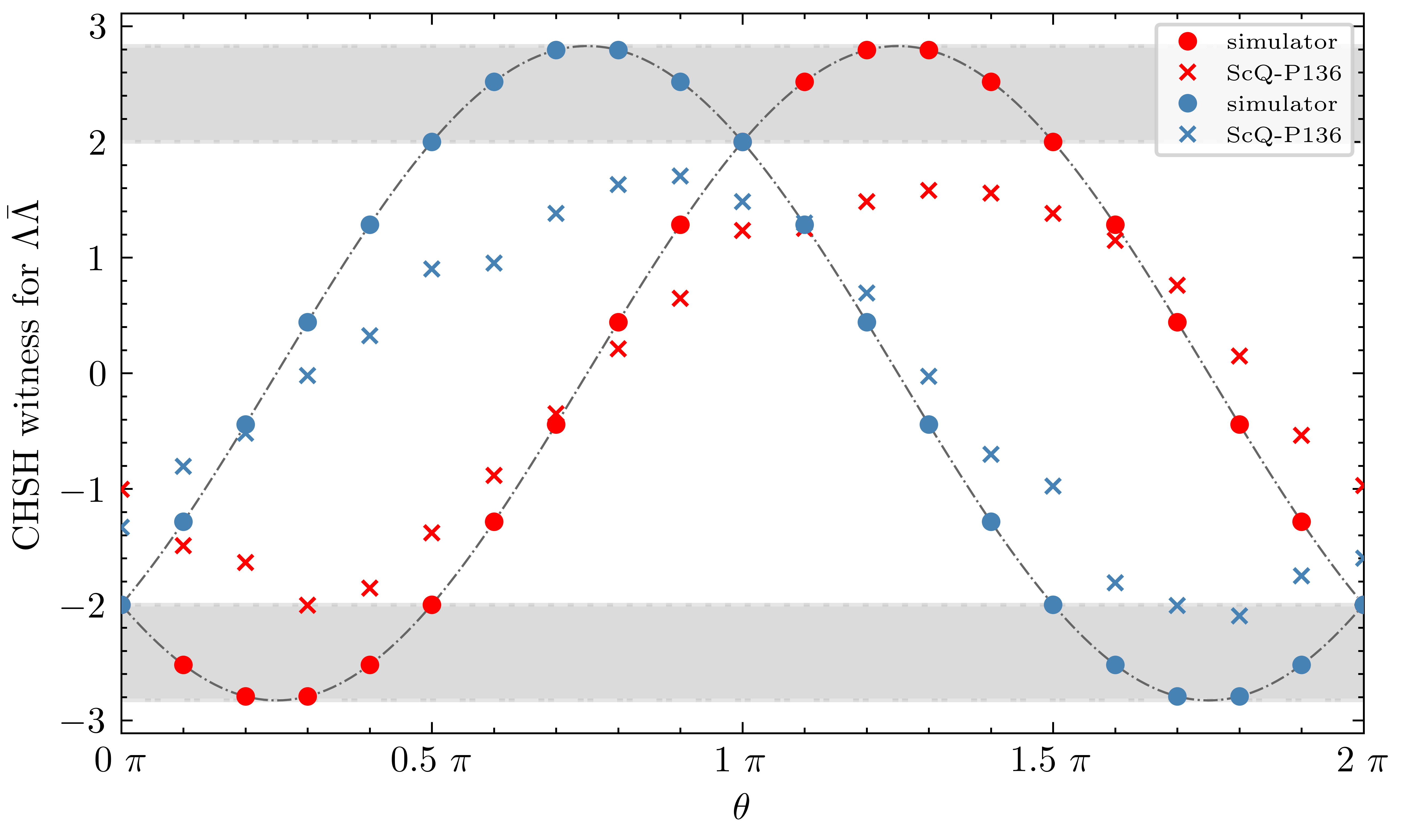
The simulation has been performed on simulators and the superconducting quantum computer Quafu developed in Beijing Academy of Quantum Information Sciences. The simulation results are shown in Fig. 2, which agree with the theoretical expectation that they enter the quantum region and reach the maximum . Thus we conclude that there is maximum violation of the CHSH inequality in from charmonium decays, which coincides with the result in Sec. IV. However, the violation of the CHSH inequality on real quantum computers turns out to be very weak. This is due to the noise in the real platform, which decreases the quantumness between two qubits. The details of our quantum simulation are shown in Appendix. A.
V.2 Simulation for depolarizing channel
As we discussed in Eq. (16), the average spin density matrix of the daughter baryon in is . In the viewpoint of QIS, the post-measurement ensemble can be interpreted as a quantum evolution characterized by the quantum channel. We notice that Eq. (16) can be regarded as a single-qubit depolarizing channel as
| (47) |
where . We have a similar form for antibaryon: with . Then the average spin density matrix for from the joint decay of can be presented as
| (48) | |||||
Since the decay processes of and are not correlated, the two-qubit channel can be described as a tensor product of two independent single-qubit depolarizing channels . From Eq. (48), the polarization vectors decrease by factors and , while the spin correlation decreases by a factor . This means that the spin correlation is suppressed in decay processes. The suppression of the spin correlation may lead to the satisfaction of the CHSH inequality, since the maximal violation also decreases by the factor , which has been discussed in Ref. [12].
We now perform a simulation based on decays . The simulation results for the channel are presented in Fig. 3. In principle, the maximum value of the Bell operator in becomes
| (49) |
with . The data for hyperon gives in PDG [32]. Thus, the maximum value is , which means the spin correlation of cannot not reach the quantum bound and does not show the property of nonlocality.
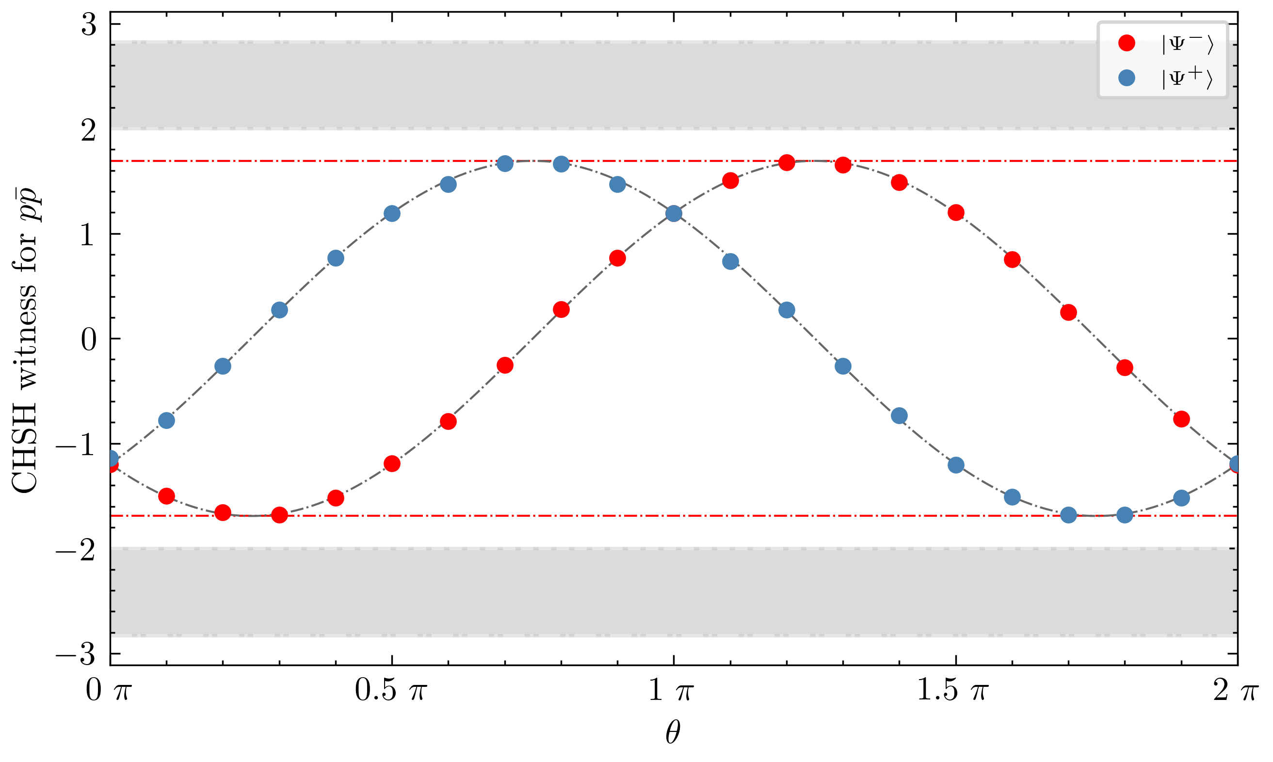
In Fig. 3, we can observe that the simulation results are in agreement with our theoretical expectation that the spin correlation in decay daughters decreases in decay processes.
VI Projective measurement and unitary evolution
In this section, we will discuss the origin of generalized measurement and its connection with particle decay/scattering processes.
In the hyperon decay , since is a pseudoscalar meson, we can neglect its quantum state. The quantum state of the mother hyperon is in the Hilbert space . The general decay process can be described by a unitary evolution called the scattering matrix in quantum field theory. In the decay, the outgoing daughter baryon is detected in the direction with the angular distribution in experiments.
From the perspective of QIS, the decay process can be described as a unitary evolution governed by the Hamiltonian (or Lagrangian) of the system, . Then the decay takes place by an emission of daughter particles in a certain direction, which indicates that a projective measurement is performed on the evolved system as , where the measurement operators are defined as projectors . Here the quantum state of the daughter baryon has been projected into the direction in momentum space. Note that the momentum magnitude is fixed by the energy-momentum conservation in the two-body decay.
According to the quantum measurement postulate discussed in Sec. II.1, the probability for finding the daughter baryon in the direction reads
| (50) |
where is just the angular distribution . In decay or scattering processes, the momenta of initial particles are pre-determined. In the decay process, the initial momentum state is denoted as by choosing the rest frame of mother particle, hence we have in Eq. (50). Since the initial momentum state is fixed, and the density matrix only contains the spin degree of freedom for the daughter baryon and can be obtained by taking the partial trace over momentum
| (51) |
where the action discards the momentum degree of freedom. Considering Eqs. (2) and (14), it can be shown that , where denotes the generalized measurement operators induced by the partial trace over momentum.
A heuristic quantum circuit in demonstrating the decay is shown as
{quantikz}\lstick& \gate[wires = 2][1.5cm]U \meterΠ_θϕ \cw\rstick
\lstick\qw\rstick
This quantum circuit gives a pedagogical illustration of the projective measurement and unitary evolution in particle decay and scattering processes in accordance with Eqs. (50, 51). The upper wire denotes the momentum state of the mother baryon , which is initialized as in the rest frame, while the lower one denotes the spin state. The unitary gate “” represents the unitary S-matrix in scattering theory. After the unitary evolution, a projective measurement is performed on the momentum state, resulting in the angular distribution of the daughter baryon. Consequently, the spin density operator in Eq. (51) is then obtained after the projective measurement.
In quantum information theory, a unitary evolution combined with projective measurements are suffice to induce a set of generalized measurements which contain both the dynamical and measurement information of the system. The generalized measurement formalism is very useful to describe decay and scattering processes in particle physics. For more details of the topic, we refer the readers to Chapter 2.2.8 of Ref. [31].
VII Summary
The particle decay processes is described as the generalized quantum measurement in quantum information theory. We consider a spin-1/2 hyperon decaying to one spin-1/2 baryon and one spin-0 meson. In this perspective, we successfully establish a correspondence between the angular distribution of the daughter baryon and the generalized measurement operator. The Bloch-Fano representation is employed to describe the quantum measurement process, which shows a direct parallelism with the decay matrices outlined in Ref. [16]. We apply this method to the joint decay of and investigate the spin correlation in as well as in systems. The quantum simulation to test the CHSH inequality on both the simulator and real quantum computer has been done. A discussion on the connection between the particle decay and the generalized quantum measurement has been given.
The generalized measurement description can be applied to a wide range of decay and scattering processes. In particular, it offers us a QIS-based tool to analyze unknown particle decays in search for new physics, such as dark matter particles. It also opens a window for testing quantum nonlocality or other quantum properties in particle decays on quantum computers. Our results can be verified in particle experiments such as BESIII [9].
Acknowledgements.
We would like to thank S. Lin, D. E. Liu and R. Venugopalan for helpful discussions. And we thank H.-Z. Xu for Quafu software and hardware supports. This work is supported by the National Natural Science Foundation of China (NSFC) under Grant Nos. 12135011, 12305010, and by the Strategic Priority Research Program of the Chinese Academy of Sciences (CAS) under Grant No. XDB34030102.Appendix A Details for quantum simulation
Through the unitary embedding introduced in Sec. V, we have the unitary operators and acting on the corresponding states as
| (52) |
where , , and with , is given in Eq. (10), and is given in Eq. (45) which are the measurement operators associated with the decay of and respectively. From Eq. (52), performing the projective measurements on the ancilla registers results in
| (53) |
which leads to the expectation value of on the ancilla qubit as
| (54) |
We see in the above formula that the expectation value associated on the qubit can be obtained from the expectation value of on the ancilla qubit . The same result holds for . Thus, the joint expectation value of reads
| (55) |
which can be directly implemented on the quantum circuit and is adopted in our test of the CHSH inequality on the quantum computer. In our simulations, the violation is ignored and the parameters are specified as and .
The Bell operator defined in Ref. [41] reads
| (56) |
where , , and are unit vectors and can be put in the plane. In our paper, the quantum states used in the test of the CHSH inequality are two Bell states . For convenience, the Bell operator in Eq. (56) is modified as
| (57) |
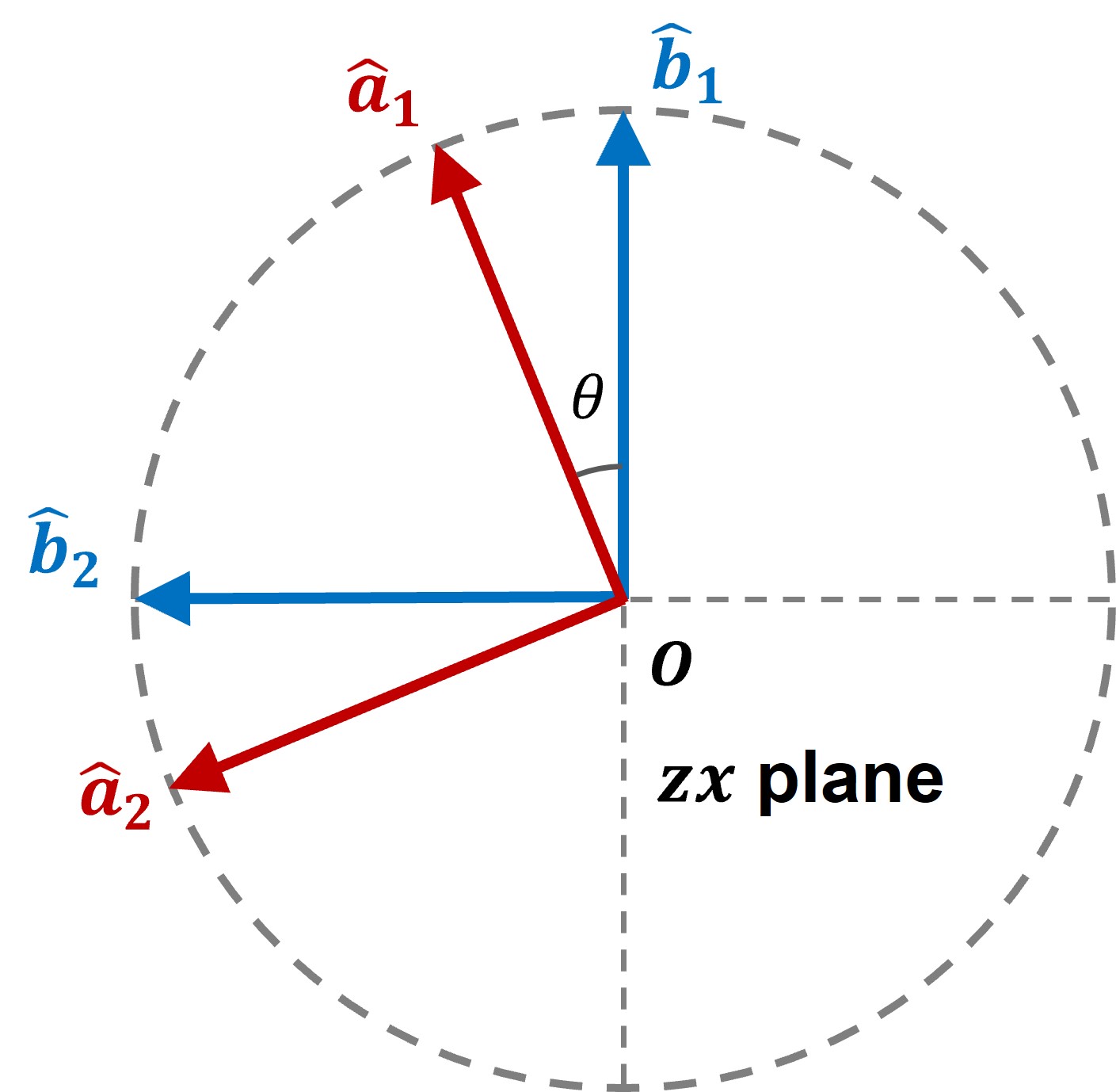
where . For further simplification, we set the angle between and is equal to , so is the angle between and . Without losing generality, we assume , , , and , see Fig. 4. The expectation values are calculated using the property with being the correlation matrix in Eq. (39). For we have , while for we have . Finally we obtain the results for as
| (58) |
& \gateH \ctrl1 \gateE \gategroup[2,steps=1,style=dashed, rounded corners,fill=blue!20,inner sep=10pt,background, ,label style=label position=below,anchor=north,yshift=-0.2cm]depolarozing channel \qw \push|p⟩
\lstick \qw \targ \gate¯E \qw \push|¯p⟩
& \gateR_y(φ) \ctrl3 \qw \qw \qw\rstick[wires=3]Trace out
\lstick \gateR_y(φ) \qw \ctrl2 \qw \qw
\lstick \gateR_y(φ) \qw \qw \ctrl1 \qw
\lstick \qw \gateX \gateY \gateZ \qw\rstick
References
- Afik and de Nova [2022] Y. Afik and J. R. M. de Nova, Quantum 6, 820 (2022).
- Altomonte and Barr [2023] C. Altomonte and A. J. Barr, Phys. Lett. B 847, 138303 (2023).
- Bell [1964] J. S. Bell, Physics Physique Fizika 1, 195 (1964).
- Clauser and Horne [1974] J. F. Clauser and M. A. Horne, Phys. Rev. D 10, 526 (1974).
- Aspect et al. [1981] A. Aspect, P. Grangier, and G. Roger, Phys. Rev. Lett. 47, 460 (1981).
- Yin et al. [2017] J. Yin, Y. Cao, Y.-H. Li, S.-K. Liao, L. Zhang, J.-G. Ren, W.-Q. Cai, W.-Y. Liu, B. Li, H. Dai, et al., Science 356, 1140 (2017).
- The BIG Bell Test Collaboration [2018] The BIG Bell Test Collaboration, Nature 557, 212 (2018).
- Aspect [2002] A. Aspect, Quantum Unspeakables: From Bell to Quantum Information, edited by R. A. Bertlmann and A. Zeilinger (Springer Berlin Heidelberg, Berlin, Heidelberg, 2002) pp. 119–153.
- Ablikim et al. [2019] M. Ablikim et al. (BESIII Collaboration), Nature Physics 15, 631 (2019).
- Törnqvist [1981] N. A. Törnqvist, Found. Phys. 11, 171 (1981).
- Khan et al. [2020] A. S. Khan, J.-L. Li, and C.-F. Qiao, Phys. Rev. D 101, 096016 (2020).
- Qian et al. [2020] C. Qian, J.-L. Li, A. S. Khan, and C.-F. Qiao, Phys. Rev. D 101, 116004 (2020).
- Chen et al. [2013] S. Chen, Y. Nakaguchi, and S. Komamiya, Prog. Theor. Exp. Phys. 2013, 063A01 (2013).
- Shi and Yang [2020] Y. Shi and J.-C. Yang, Eur. Phys. J. C 80, 116 (2020).
- Perotti et al. [2019] E. Perotti, G. Fäldt, A. Kupsc, S. Leupold, and J. J. Song, Phys. Rev. D 99, 056008 (2019).
- Batozskaya et al. [2023] V. Batozskaya, A. Kupsc, N. Salone, and J. Wiechnik, Phys. Rev. D 108, 016011 (2023).
- Gong et al. [2022] W. Gong, G. Parida, Z. Tu, and R. Venugopalan, Phys. Rev. D 106, L031501 (2022).
- Aoude et al. [2022] R. Aoude, E. Madge, F. Maltoni, and L. Mantani, Phys. Rev. D 106, 055007 (2022).
- Afik and de Nova [2023] Y. Afik and J. R. M. de Nova, Phys. Rev. Lett. 130, 221801 (2023).
- Fabbrichesi et al. [2021] M. Fabbrichesi, R. Floreanini, and G. Panizzo, Phys. Rev. Lett. 127, 161801 (2021).
- Afik and de Nova [2021] Y. Afik and J. R. M. de Nova, Eur. Phys. J. P 136, 907 (2021).
- Fabbrichesi et al. [2023a] M. Fabbrichesi, R. Floreanini, and E. Gabrielli, The European Physical Journal C 83 (2023a).
- Barr [2022] A. J. Barr, Physics Letters B 825, 136866 (2022).
- Barr et al. [2023] A. J. Barr, P. Caban, and J. Rembieliński, Quantum 7, 1070 (2023).
- Fabbrichesi et al. [2023b] M. Fabbrichesi, R. Floreanini, E. Gabrielli, and L. Marzola, The European Physical Journal C 83 (2023b).
- Ashby-Pickering et al. [2023] R. Ashby-Pickering, A. J. Barr, and A. Wierzchucka, J. High Ener. Phys. 2023, 20 (2023).
- Barata et al. [2023] J. Barata, W. Gong, and R. Venugopalan, Realtime dynamics of hyperon spin correlations from string fragmentation in a deformed four-flavor schwinger model (2023), arXiv:2308.13596 [hep-ph] .
- Pang et al. [2016] L.-G. Pang, H. Petersen, Q. Wang, and X.-N. Wang, Phys. Rev. Lett. 117, 192301 (2016).
- Lv et al. [2024] J.-P. Lv, Z.-H. Yu, Z.-T. Liang, Q. Wang, and X.-N. Wang, Global quark spin correlations in relativistic heavy ion collisions (2024), arXiv:2402.13721 [hep-ph] .
- Hao et al. [2010] X.-Q. Hao, H.-W. Ke, Y.-B. Ding, P.-N. Shen, and X.-Q. Li, Chin. Phys. C 34, 311 (2010).
- M. A. Nielsen and I. L. Chuang [2015] M. A. Nielsen and I. L. Chuang, Quantum Computation and Quantum Information (Cambridge University Press, Cambridge, 2015).
- Particle Data Group [2020] Particle Data Group, Progress of Theoretical and Experimental Physics 2020, 083C01 (2020).
- Lee and Yang [1957] T. D. Lee and C. N. Yang, Phys. Rev. 108, 1645 (1957).
- Cronin and Overseth [1963] J. W. Cronin and O. E. Overseth, Phys. Rev. 129, 1795 (1963).
- Fano [1957] U. Fano, Rev. Mod. Phys. 29, 74 (1957).
- Fano [1983] U. Fano, Rev. Mod. Phys. 55, 855 (1983).
- Benenti and Strini [2011] G. Benenti and G. Strini, Int. J. Quant. Info. 9, 73 (2011).
- Jacob and Wick [1959] M. Jacob and G. C. Wick, Annals of Physics 7, 404 (1959).
- Baumgart and Tweedie [2013] M. Baumgart and B. Tweedie, J. High Ener. Phys. 2013, 1 (2013).
- Chen and Ping [2020] H. Chen and R.-G. Ping, Phys. Rev. D 102, 016021 (2020).
- Horodecki et al. [1995] R. Horodecki, P. Horodecki, and M. Horodecki, Phys. Lett. A 200, 340 (1995).