Searching a Lightweight Network Architecture for Thermal Infrared Pedestrian Tracking

Abstract

Manually-designed network architectures for thermal infrared pedestrian tracking (TIR-PT) require substantial effort from human experts. Neural networks with ResNet backbones are popular for TIR-PT. However, TIR-PT is a tracking task and more challenging than classification and detection. This paper makes an early attempt to search an optimal network architecture for TIR-PT automatically, employing single-bottom and dual-bottom cells as basic search units and incorporating eight operation candidates within the search space. To expedite the search process, a random channel selection strategy is employed prior to assessing operation candidates. Classification, batch hard triplet, and center loss are jointly used to retrain the searched architecture. The outcome is a high-performance network architecture that is both parameter- and computation-efficient. Extensive experiments proved the effectiveness of the automated method.

I Introduction

Thermal infrared pedestrian tracking (TIR-PT) is an active research field in computer vision and draws increasing interest in autonomous driving and underwater vehicles. It is generally treated as an object detection problem that intends to follow a specific pedestrian in TIR video sequences [1].

Deep convolutional neural networks (CNNs) have been widely used in TIR-PT to extract features. Most of the CNNs of TIR-PT adopt typical networks such as AlexNet [2], VGGNet [3], and ResNet [4] as the backbone architecture, then integrate more layers to use deep features. For example, MMNet [5] implemented a multi-task matching network based on the AlexNet to learn object-specific discriminative and fine-grained correlation feature maps of TIR pedestrians. LMSCO [6] integrate motion information of the pedestrian into VGGNet to overcome the background clutter and motion blur of the TIR image. ASTMT [7] designed an aligned spatial-temporal memory network based on ResNet to take advantage of learning scene information for pedestrian localization. The well-performance handcrafted neural networks require substantial effort from human experts. However, these backbones were initially designed for image classification and thus have many redundant parts when transferred to different tasks. Since TIR-PT is an instance-level detection task, we hope to find a specific architecture suitable for it.

Neural architecture search (NAS) has recently attracted wide attention in computer vision [8, 9]. NAS is an important advance that automates neural network designing. Given a search space, NAS methods aim to search a high-performance architecture with specific search strategies. In this paper, we attempt to search for an efficient network architecture for the TIR-PT task automatically. Conventional NAS methods cost intensive computation and memory. For instance, the reinforcement learning (RL)-based NASNet proposed by Zoph et al.  [10] takes 2000 GPU days to search and evaluate neural networks. AmoebaNet [11] is a well-known regularized evolution method. It costs 3150 GPU days to find a suitable architecture. We employ the recent state-of-the-art tracker DiMP [12] as our baseline and use a differentiable searching manner inspired by [13] to learn preferable network architecture for TIR-PT tasks. We relax the discrete search space to be continuous to optimize the architecture by gradient descent, and design a two-stage (search and retrain) method for TIR-PT, as shown in Fig.1. In the first stage, operation candidates in the search space are used to discover the basic architecture cells (or blocks). Then, the overall network architecture is constructed by stacking cells. Similar to the attention mechanism, apart from updating normal operation (such as convolutions) parameters $\omega$, we also need to update architecture parameters $\alpha$, an attention matrix representing the importance of each operation. Since it is a bi-level optimization problem, $\alpha$ and $\omega$ can be thus updated alternately. Though the differentiable method is relatively faster than other NAS, it still costs a lot of storage. Therefore, we randomly select channels and feed them into operation candidates to reduce computation, as suggested by [14]. The efficiency of the search process can be improved in this way. As for the second stage, we chose the most critical operation to form the final network architecture, similar to network pruning. We use joint supervision of classification, batch hard triplet, and center loss to learn more discriminative features to retrain the searched network architecture. Our contributions can be summarized as follows.

• We construct single-bottom and dual-bottom cells as basic units, and stack them together to search a network architecture.

• We randomly select some channels and feed them into operation candidates to accelerate the search process.

• We explore joint supervision to retrain the searched architecture to handle the challenging scenarios of TIR-PT.

• We conduct extensive experiments to demonstrate the effectiveness and efficiency of our proposed method.

II The proposed method

II-A Basic search units

II-A1 Single-bottom Cells

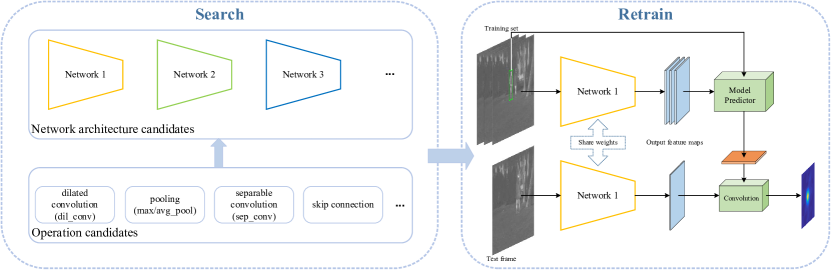
Figure 1: Overview of the proposed TIR-PT method.

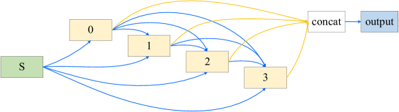
Figure 2: Pipeline of the single-bottom cell.

Figure 3: Pipeline of the dual-bottom cell.

We search for two kinds of computation cells (normal and reduction), then stack them together to form a convolutional network. The function of the normal cell is to enhance the expressive performance of the model. Reduction cells are used for reducing the size of feature maps to half of the current input and doubling the number of channels. A cell is a directed acyclic graph (DAG) with ordered sequence nodes. As illustrated in Fig.2, we propose an architecture with only one input (single-bottom) consisting of 6 nodes in one cell. Input node S represents previous features. Nodes 0, 1, 2, and 3 are intermediate features that are concatenated as the output of the current cell.

II-A2 Dual-bottom Cells

The performance of single-bottom architecture may not be good enough because only the most crucial edge is left during inference to simplify cells and reduce calculations. To preserve more information, the dual-bottom cell is considered to balance performance and computing. The dual-bottom cell is shown in Fig.3. The current input nodes S0 and S1 are outputs from the previous two layers. There are seven nodes for one cell. Search space is the same with single-bottom cells.

II-B Operation candidates

We define 8 operation candidates (search space) for each blue edge in Figs.2 and 3: none, 3$\times$3 max pooling, 3$\times$3 average pooling, 3$\times$3 depth-wise separable convolution, 5$\times$5 depth-wise separable convolution, skip connection, 3$\times$3 dilated convolution, 5$\times$5 dilated convolution. The normal and reduction cells are stacked repeatedly to form the final architecture. We keep the most crucial edge in inference to simplify architectures and reduce computations. We use a differential architecture search method to convert all discrete operations into a continuous search space by a softmax function. In this way, the architecture search task is simplified to learn a set of continuous variables,

$$\bar{o}^{(i,j)}(x)=\sum_{o\in\mathcal{O}}\frac{\exp(\alpha_{o}^{(i,j)})}{\sum_{o^{\prime}\in\mathcal{O}}\exp(\alpha_{o^{\prime}}^{(i,j)})}o(x)$$ (1)

where $x$ represents feature maps, $\mathcal{O}$ denotes the search space where each operation candidate $o\in\mathcal{O}$ represents convolution or pooling.

The continuous variables $a_{o}^{(i,j)}$ indicates the mixing weight associated with the operation $o$ between nodes $i$ and $j$ and forms a matrix $\alpha$. For Instance, dual-bottom cells are encoded as a matrix with 14 rows (edges) and 8 columns (operation candidates), while single-bottom cells are encoded as a matrix with 10 rows and 8 columns. The matrix represents the topology structure for a cell, named architecture parameters. Other operation parameters are marked as $\omega$. As for $\alpha$, it needs to optimize two kinds of the matrix where $\alpha_{1}$ is shared by all the normal cells and $\alpha_{2}$ is shared by all the reduction cells. Searching architecture parameters $\alpha$ and the operation parameters $\omega$ is a bi-level optimization problem, they are thus updated alternately.

II-C Random Channel Selection

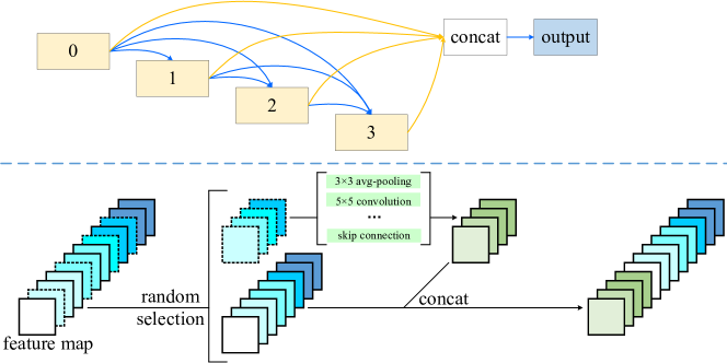
Figure 4: Illustration of the random channel selection.

Calculating and saving all feature maps during the search process takes a lot of computing resources. The differentiable NAS still suffers from the issue of high GPU memory consumption. In order to solve this problem and speed up the search process with limited resources, we randomly select a subset of channels and then send them into operation candidates while keeping the rest unchanged. The sampling rate of the channel is $1/4$. Finally, we concatenate the features depth-wise, as shown in Fig.4. They are calculated as follows,

$$\bar{o}^{(i,j)}(x;r^{(i,j)}) =\sum_{o\in\mathcal{O}}\frac{\exp(\alpha_{o}^{(i,j)})}{\sum_{o^{\prime}\in\mathcal{O}}\exp(\alpha_{o^{\prime}}^{(i,j)})}o(r^{(i,j)}x)$$ (2)

$$+(1-r^{(i,j)})x$$

where $\alpha$ is the searched architecture. $r^{(i,j)}x$ and $(1-r^{(i,j)})x$ respectively represent selected channels and the rest channels.

II-D Joint Supervision

We retrain the searched architecture with joint supervision. To keep the pedestrian identity and separate the foreground from the background, we take a classification loss as the first supervision as,

$$\mathcal{L}_{CLS}=-\sum_{k}\big{[}y_{k}\log(h_{k})+(1-y_{k})\log(1-h_{k})\big{]}$$ (3)

where $y_{k}$ denote the ground-truth label of the $k$-th sample, $h_{k}$ is denoted as the probability belong to the foreground predicted by the searched network.

TIR-PT is more complex than object recognition and classification because of the great intra-variations in each class and the variety of factors such as thermal crossover and intensity variation. We take triplets into account so that the output feature maps from the searched neural network can be utilized directly. Sample anchor, positive and negative randomly, may render the combinations of triplets to grow cubically as the dataset gets larger for classical triplets. It is impractical to train the model for a long enough time. In order to mine hard triplets, we adopt batch hard triplet loss as a supervision. For each batch, we sample $M$ pedestrian sequences (a.k.a., classes) randomly from the training dataset and then pick $N$ image frames for each class. Therefore, a batch contains $M\times N$ image frames. We calculate the distance between feature maps extract from different image frames, hard positive (pedestrians with remarkably different appearances or scales picked from the same video sequence), and hard negative (pedestrians with similar appearances or scales picked from different video sequences) within the batch. The batch hard triplet loss function is presented as follows.

$$\mathcal{L}_{BHTri}=\sum_{m=1}^{M}\sum_{n=1}^{N} \big{[}\delta+\max_{p=1,\ldots,N}\mathcal{D}(f_{\alpha}(x_{m}^{n}),f_{\alpha}(x_{m}^{p}))$$ (4)

$$-\min_{\begin{subarray}{c}s=1,\ldots,M\\ t=1,\ldots,N\\ s\neq m\end{subarray}}\mathcal{D}(f_{\alpha}(x_{m}^{n}),f_{\alpha}(x_{s}^{t}))\big{]}_{+}$$

where $\delta$ is margin which equals 0.3, $\mathcal{D}$ is a metric function measuring distances in the embedding space, $f_{\alpha}$ denote distance and feature maps, $x_{n}^{m}$ denotes $n$-th image frames of $m$-th pedestrian video sequence, $[u]_{+}$ represents $\max(u,0)$.

We try to narrow the gap between features extracted from the same pedestrian class with different image frames. We need to make the features of the same class form a single cluster, and the same pedestrian is also required to collapse to a small point eventually. The distances of the intra-class may be further than those of the inter-class under the supervision of triplet loss. In order to minimize the intra-class distances, we utilize center loss to learn a center for features of each class. The function is computed as follows,

$$\mathcal{L}_{CT}=\sum_{u=1}^{\mathcal{B}}\mathcal{D}(f_{\alpha}(x_{h_{u}}),f_{\alpha}(x_{y_{u}}))$$ (5)

where $\mathcal{B}$ is the batch size, $f_{\alpha}(x_{h_{u}})$ and $f_{\alpha}(x_{y_{u}})$ represent the feature maps extracted from the predicted and the ground-truth bounding boxes of the $u$-th sample, respectively.

We train the searched architecture under joint supervision of classification loss, batch hard triple loss, and center loss as follows,

$$\mathcal{L}=\mathcal{L}_{CLS}+\mathcal{L}_{BHTri}+\gamma\mathcal{L}_{CT}$$ (6)

where $\gamma$ is used for balancing the center loss.

III Experiments

III-A Datasets and Metrics

III-A1 Datasets

Two popular TIR-PT datasets are used in our experiments: LSOTB-TIR [15] and PTB-TIR [16]. LSOTB-TIR includes 1,280 TIR video sequences for evaluation and 120 for training, the number of total image frames is more than 600K. PTB-TIR consists of 60 TIR pedestrian video sequences with a total of 30K image frames.

III-A2 Metrics

LSOTB-TIR uses precision, success, and normalized precision as evaluation metrics. Precision is the ratio of frames with center location error between the predicted bounding box and the ground truth below a specified threshold (20 pixels) relative to the size of the video sequence. Normalized precision adjusts precision by considering the scale of the pedestrian or the size of the image frame. Success evaluates the overlap between the predicted bounding box and the ground truth, usually represented as the area under the curve (AUC) in a success plot. PTB-TIR used the same precision and success as LSOTB-TIR to report the tracking performance.

III-B Implementation Details

In the searching process, random erasing, normalization, random horizontal flipping with 0.5, and padding the resized image 10 pixels with zero values are applied as the data augmentation. We hold out half of the training data to update architecture parameters $\alpha$. The other half of the training data can be viewed as a search validation set used to update operation parameters $\omega$. We utilize Adam [17] as the optimizer for $\alpha$, with an initial learning rate of 0.02, decay rates $\beta_{1}=0.5$ and $\beta_{2}=0.999$. We use momentum Stochastic Gradient Descent (SGD) to optimize the weights $\omega$. The initial learning rate starts from 0.1 and anneals down to 0.001 following a cosine schedule without restart for each epoch [18]. We search architecture for 200 epochs.

In the retraining process, we apply horizontal flip and normalization as data augmentation. SGD with momentum is deployed as the optimizer with an initial learning rate of 0.1 decayed with a cosine annealing. Each batch contains 8 pedestrians ($M$), and each pedestrian has 8 image frames ($N$), resulting in a batch size of 64.

The training dataset of LSOTB-TIR [15] is utilized to search and retrain the network architecture, we resize each training and test regions to 128$\times$128 and 256$\times$256. Except for the aforementioned details, the rest of the hyperparameters and configurations are are the same as DiMP [12]. We implement our method in Python using PyTorch with an instance with an Intel^® Xeon^® Gold 6148v4 CPU @ 2.2 GHz CPU with 256 GB RAM and a NVIDIA^® Tesla^® V100-SXM2 GPU with 16 GB VRAM.

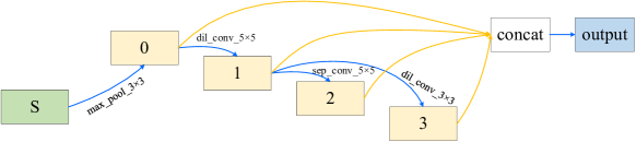
Figure 5: Illustration of the searched normal single-bottom cell.

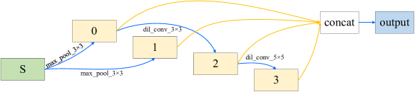
Figure 6: Illustration of the searched reduction single-bottom cell.

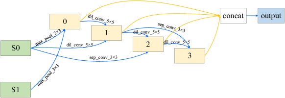
Figure 7: Illustration of the searched normal dual-bottom cell.

Figure 8: Illustration of the searched reduction dual-bottom cell.

TABLE I: Ablation studies of the proposed method on the LSOTB-TIR benchmark dataset. S-c, D-c, CH, $\mathcal{L}_{CLS}$, $\mathcal{L}_{BHTri}$, and $\mathcal{L}_{CT}$ denote the single-bottom cell, dual-bottom cell, random channel selection, classification loss, batch triplet loss, and center loss, respectively.

Method configurations						Precision	Success	Norm. Precision	Params	FLOPs	GPU days
S-c	D-c	CH	$\mathcal{L}_{CLS}$	$\mathcal{L}_{BHTri}$	$\mathcal{L}_{CT}$
✓			✓			0.768	0.640	0.697	2.96 M	0.78 G	3.3
✓	✓		✓			0.783	0.656	0.715	4.73 M	1.35 G
✓	✓	✓	✓			0.785	0.656	0.715	5.31 M	1.58 G	1.9
✓	✓	✓	✓	✓		0.792	0.665	0.717
✓	✓	✓	✓	✓	✓	0.805	0.669	0.720

TABLE II: Comparison of the state-of-the-art methods on the LSOTB-TIR and PTB-TIR benchmark datasets.

Methods	LSOTB-TIR			PTB-TIR
	Precision	Success	Norm. Precision	Precision	Success
DiMP [12]	0.780	0.616	0.703	0.749	0.618
ECO-STIR [19]	0.750	0.616	0.672	0.830	0.617
HSSNet [20]	0.515	0.409	0.488	0.689	0.468
MCFTS [21]	0.635	0.479	0.546	0.690	0.492
MDNet [22]	0.750	0.601	0.686	0.817	0.593
MLSSNet [23]	0.596	0.459	0.549	0.741	0.539
MMNet [5]	0.582	0.476	0.539	0.783	0.557
TADT [24]	0.710	0.587	0.635	0.740	0.560
Ours	0.805	0.669	0.720	0.776	0.643

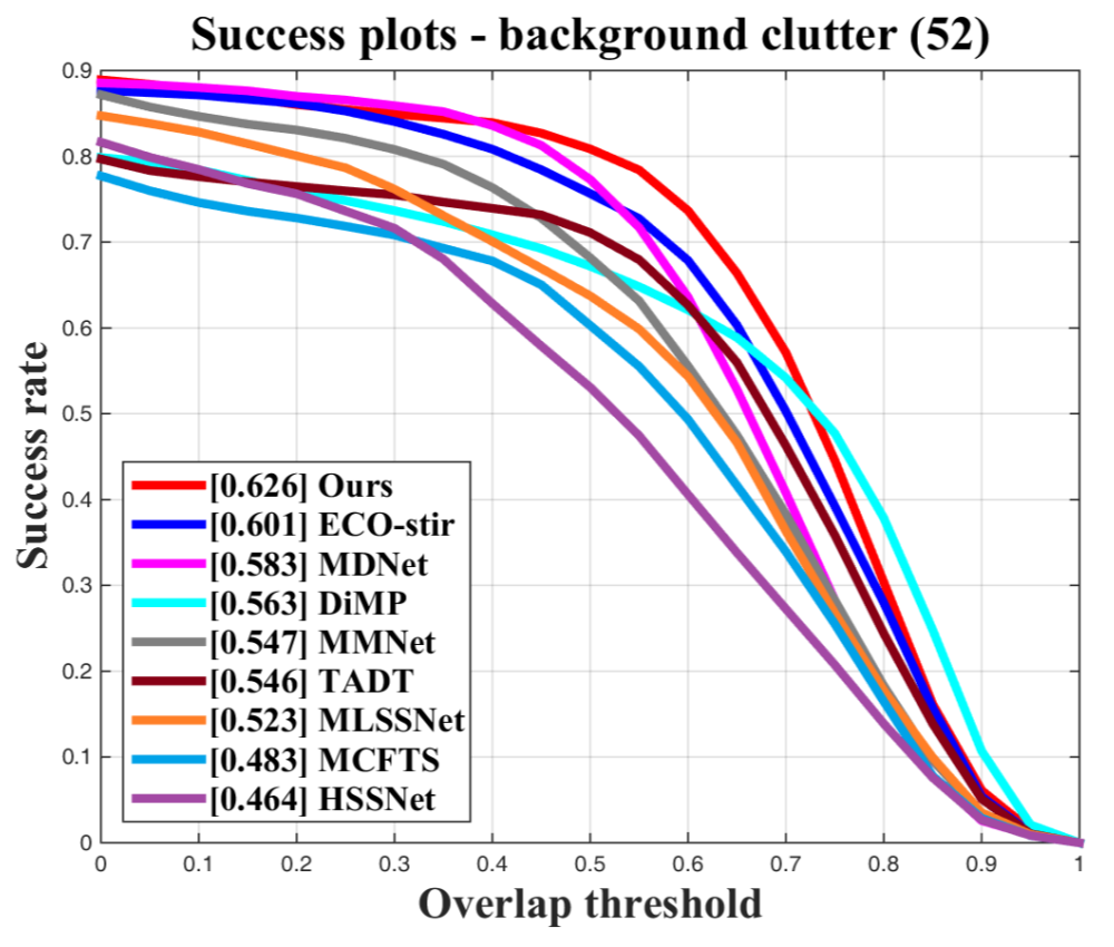
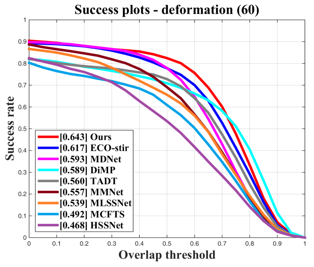
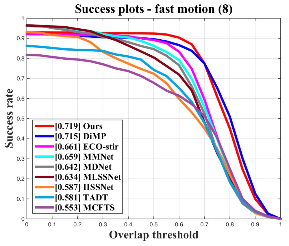
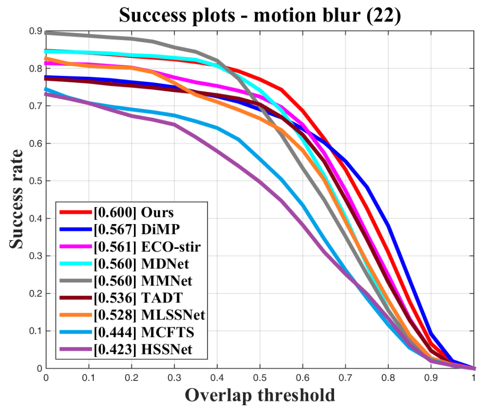
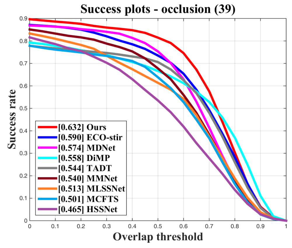
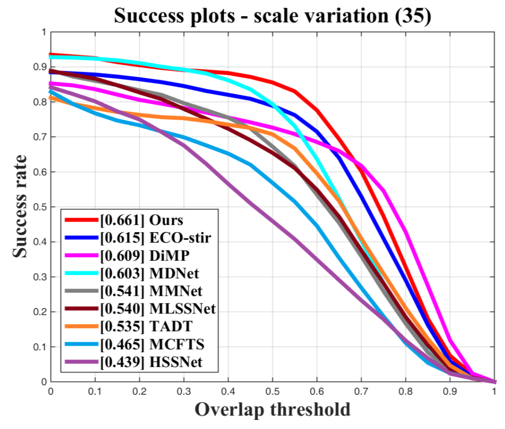
Figure 9: Comparison of the state-of-the-art methods on six PTB-TIR challenge subsets.

III-C Ablation Studies

III-C1 Effects of single-bottom and dual-bottom cells

The searched normal single-bottom cell is illustrated in Fig.5. To simplify architecture, only the most crucial edge is considered as input for the next layer. For instance, instead of feeding nodes S, 0, 1, and 2 into node 3, we only feed node 2 into node 3 through a 5$\times$5 dilated convolution because the architecture parameters between nodes 2 and 3 are the largest. It’s similar to attention-based pruning. The same principle applies to the reduction single-bottom cell, as shown in Fig.6. The searched normal and reduction dual-bottom cells are shown in Figs.7 and 8, respectively, which take two nodes as the input. The dual-bottom cells are more complicated than single-bottom cells. We retrain the searched architecture (random initialization) to evaluate the performance of the model. The results are shown in Table I. The single-bottom cells are very simple and have only one input, thus losing a lot of information from previous layers. Therefore, the parameters and FLOPs are small, while precision and rank are not good enough. As for the dual-bottom cells, they balance the accuracy and parameters, thus significantly improving the tracking performance.

III-C2 Effect of selecting channel randomly

We randomly select some channels and feed them into 8 operation candidates to reduce memory consumption and speed up the search process. The retrain process follows the setting of calculating all channels. We stack 16 cells (12 normal and 4 reduction cells) to form the final dual-bottom architecture. It takes 1.9 GPU days to search cells with randomly selected channels, faster than computing all channels (3.3 GPU days). The method of randomly selecting channels performs a more efficient search without compromising the performance. In this way, we can also search architecture with larger batch sizes.

III-C3 Effects of joint supervision

The batch triplet loss and center loss make use of feature maps before model prediction. The model under the joint supervision of classification, batch hard triplet, and center loss outperforms the model only with classificant loss by a significant margin, confirming the advantage of the joint loss function. As for the batch triplet loss, it obtains +0.7%/+0.9%/+0.2% improvements on the precision/success/normalization precision scores, respectively. It is obvious that the center loss plays a vital role due to considerable intra-class variations, promoting performance with 0.4% on the success score and 1.3% on the precision score.

III-D State-of-the-art Comparison

We construct a TIR-PT model that utilizes the final searched and retrained network architecture and compare it with the state-of-the-art methods, including DiMP [12], ECO-STIR [19], HSSNet [20], MCFTS [21], MDNet [22], MLSSNet [23], MMNet [5], and TADT [24], on the LSOTB-TIR [15] and PTB-TIR [16] benchmark datasets. Comparison results are shown in Table II, our method achieves competitive performance.

LSOTB-TIR [15] is a more comprehensive benchmark dataset due to the more intra-class variations of pedestrians in more challenging scenarios, such as background clutter, deformation, motion blur, and occlusion. It is evident that our method achieves the best performance compared with other state-of-the-art methods, the precision/success/normalized precision scores reach 0.805/0.669/0.720, which improves the baseline method, DiMP [12], by 2.5%/5.3%/1.7%, respectively. Compared with MMNet [5], which learns dual-level deep representation for TIR tracking, our method has more than 18% improvement of all metrics on LSOTB-TIR.

The TIR-PT model searched and retrained on the LSOTB-TIR dataset can be indeed transferable to the PTB-TIR [16] dataset, achieves the best success score of 0.641 and a comparable precision score of 0.776, outperforming DiMP with relative gains of 2.7% and 2.3%, respectively. ECO-STIR [19] uses ResNet-50 as its base network and utilizes synthetic TIR data generated from RGB data to train the model, which obtains the best precision score of 0.830, with a relative gain of 5.4% compared to our method. Still, its success score is inferior to ours, with a degradation of 2.4%. We also conduct evaluations on six challenge scenarios often occurring in pedestrian tracking, as shown in Fig.9. Our method achieves the best performance on all these challenges.

The above experimental result proves that our method can search a more effective and efficient network architecture for the TIR-PT task.

IV Conclusion

In this paper, we employ a NAS approach to find an effective network architecture for the TIR-PT task. We design single-bottom and dual-bottom cells as basic searching units and randomly select channels to reduce computation and memory and feed them into operation candidates. Furthermore, the joint supervision of classification, batch hard triplet, and center loss are introduced to learn more discriminative features. The overall performance of our method outperforms the state-of-the-art methods with less computation. Extensive experiments demonstrate the effectiveness and efficiency of our proposed method.

References

- [1] X. Zhong, T. Lu, W. Huang, M. Ye, X. Jia, and C.-W. Lin, “Grayscale enhancement colorization network for visible-infrared person re-identification,” IEEE Transactions on Circuits and Systems for Video Technology, vol. 32, no. 3, pp. 1418–1430, 2022.
- [2] A. Krizhevsky, I. Sutskever, and G. E. Hinton, “Imagenet classification with deep convolutional neural networks,” in Advances in Neural Information Processing Systems, 2012, pp. 1097–1105.
- [3] K. Simonyan and A. Zisserman, “Very deep convolutional networks for large-scale image recognition,” arXiv preprint arXiv:1409.1556v6, 2015.
- [4] K. He, X. Zhang, S. Ren, and J. Sun, “Deep residual learning for image recognition,” in IEEE Conference on Computer Vision and Pattern Recognition, 2016, pp. 770–778.
- [5] Q. Liu, D. Yuan, N. Fan, P. Gao, X. Li, and Z. He, “Learning dual-level deep representation for thermal infrared tracking,” IEEE Transactions on Multimedia, vol. 25, pp. 1269–1281, 2022.
- [6] P. Gao, Y. Ma, K. Song, C. Li, F. Wang, and L. Xiao, “Large margin structured convolution operator for thermal infrared object tracking,” in IEEE International Conference on Pattern Recognition, 2018, pp. 2380–2385.
- [7] D. Yuan, X. Shu, Q. Liu, and Z. He, “Aligned spatial-temporal memory network for thermal infrared target tracking,” IEEE Transactions on Circuits and Systems II: Express Briefs, vol. 70, no. 3, pp. 1224–1228, 2022.
- [8] H. Huang, L. Shen, C. He, W. Dong, and W. Liu, “Differentiable neural architecture search for extremely lightweight image super-resolution,” IEEE Transactions on Circuits and Systems for Video Technology, vol. 33, no. 6, pp. 2672–2682, 2023.
- [9] L. Cai, Y. Fu, W. Huo, Y. Xiang, T. Zhu, Y. Zhang, H. Zeng, and D. Zeng, “Multiscale attentive image de-raining networks via neural architecture search,” IEEE Transactions on Circuits and Systems for Video Technology, vol. 33, no. 2, pp. 618–633, 2023.
- [10] B. Zoph, V. Vasudevan, J. Shlens, and Q. V. Le, “Learning transferable architectures for scalable image recognition,” in IEEE Conference on Computer Vision and Pattern Recognition, 2018, pp. 8697–8710.
- [11] E. Real, A. Aggarwal, Y. Huang, and Q. V. Le, “Regularized evolution for image classifier architecture search,” in AAAI Conference on Artificial Intelligence, vol. 33, no. 01, 2019, pp. 4780–4789.
- [12] G. Bhat, M. Danelljan, L. V. Gool, and R. Timofte, “Learning discriminative model prediction for tracking,” in International Conference on Computer Vision (ICCV). IEEE, 2019, pp. 6182–6191.
- [13] P. Gao, X. Liu, H.-C. Sang, Y. Wang, and F. Wang, “Efficient and lightweight visual tracking with differentiable neural architecture search,” Electronics, vol. 12, no. 17, p. 3623, 2023.
- [14] Y. Xu, L. Xie, X. Zhang, X. Chen, G.-J. Qi, Q. Tian, and H. Xiong, “Pc-darts: Partial channel connections for memory-efficient architecture search,” in International Conference on Learning Representations, 2019.
- [15] Q. Liu, X. Li, D. Yuan, C. Yang, X. Chang, and Z. He, “Lsotb-tir: A large-scale high-diversity thermal infrared single object tracking benchmark,” IEEE Transactions on Neural Networks and Learning Systems, 2023.
- [16] Q. Liu, Z. He, X. Li, and Y. Zheng, “Ptb-tir: A thermal infrared pedestrian tracking benchmark,” IEEE Transactions on Multimedia, vol. 22, no. 3, pp. 666–675, 2019.
- [17] D. P. Kingma and J. Ba, “Adam: A method for stochastic optimization,” arXiv preprint arXiv:1412.6980, 2014.
- [18] I. Loshchilov and F. Hutter, “Sgdr: Stochastic gradient descent with warm restarts,” arXiv preprint arXiv:1608.03983, 2016.
- [19] L. Zhang, A. Gonzalez-Garcia, J. Van De Weijer, M. Danelljan, and F. S. Khan, “Synthetic data generation for end-to-end thermal infrared tracking,” IEEE Transactions on Image Processing, vol. 28, no. 4, pp. 1837–1850, 2018.
- [20] X. Li, Q. Liu, N. Fan, Z. He, and H. Wang, “Hierarchical spatial-aware siamese network for thermal infrared object tracking,” Knowledge-Based Systems, vol. 166, pp. 71–81, 2019.
- [21] Q. Liu, X. Lu, Z. He, C. Zhang, and W.-S. Chen, “Deep convolutional neural networks for thermal infrared object tracking,” Knowledge-Based Systems, vol. 134, pp. 189–198, 2017.
- [22] H. Nam and B. Han, “Learning multi-domain convolutional neural networks for visual tracking,” in IEEE/CVF Conference on Computer Vision and Pattern Recognition (CVPR). IEEE, 2016, pp. 4293–4302.
- [23] Q. Liu, X. Li, Z. He, N. Fan, D. Yuan, and H. Wang, “Learning deep multi-level similarity for thermal infrared object tracking,” IEEE Transactions on Multimedia, vol. 23, pp. 2114–2126, 2020.
- [24] X. Li, C. Ma, B. Wu, Z. He, and M.-H. Yang, “Target-aware deep tracking,” in Proceedings of the IEEE/CVF conference on computer vision and pattern recognition, 2019, pp. 1369–1378.