Data depth functions for non-standard data by use of formal concept analysis

Abstract

Data depth functions have been intensively studied for normed vector spaces. However, a discussion on depth functions on data where one specific data structure cannot be presupposed is lacking. In this article, we introduce a notion of depth functions for data types that are not given in statistical standard data formats and therefore we do not have one specific data structure. We call such data in general non-standard data. To achieve this, we represent the data via formal concept analysis which leads to a unified data representation. Besides introducing depth functions for non-standard data using formal concept analysis, we give a systematic basis by introducing structural properties. Furthermore, we embed the generalised Tukey depth into our concept of data depth and analyse it using the introduced structural properties. Thus, this article provides the mathematical formalisation of centrality and outlyingness for non-standard data and therefore increases the spaces centrality is currently discussed. In particular, it gives a basis to define further depth functions and statistical inference methods for non-standard data.

1 Introduction

Data depth functions generalise the concept of centrality and outlyingness to multivariate data and provide therefore a useful concept to define nonparametric and robust statistical methods. To achieve this, depth functions denote the center and outlying areas based on an underlying distribution or a data cloud. Moreover, they classify how near other areas are to the outlying or center ones. This results in a center-outward order of the data points. Since there does not exist one unique perspective on centrality, several different depth functions on $\mathbb{R}^{d}$ have been developed. Some examples are simplicial depth, see [14], zonoid depth, see [9], or Tukey depth, see [22, 5]. To give a systematic basis on the notion of depth functions [23] and [15] set up properties to mathematically formalise the existing intuition about centrality and outlyingness in $\mathbb{R}^{d}$. In addition to $\mathbb{R}^{d}$, the scope of data types on which depth functions are defined increased in the last years. For example, in [11] the authors discuss properties of depth functions on functional data. In recent years, this concept has been used to construct statistical methods and to analyse different application settings. For example [13, 18] developed statistical nonparametric and robust tests using depth functions. Using the robust central-outward order [17] studied anomaly detection. In [4], data depth functions are used to visualise and describe features of hydrologic events given two real world streamflow data sets from Canada.

However, all these depth functions and analyses have in common that they build on spaces that have a strong underlying structure, like Banach spaces. Thus, to apply the concept of depth and resulting statistical methods, the data has to be embedded into statistical standard data formats, like numeric or nominal. The aim of this article is to take the next step and consider depth functions without assuming one specific data type in advance. This includes data types like, e.g., set of partial orders or mixed spatial and ordinal data. We call data that cannot be embedded into statistical standard data formats non-standard data. To give a notion of centrality and outlyingness for non-standard data, a unified data representation is needed. Therefore, we use the theory of formal concept analysis which transforms the data set into a closure system on the entire data set itself. This gives us a unified, flexible, and general applicable specification for different data structures. In particular, it does not force the user to add assumptions on the data which are not necessarily fulfilled. We use this unified representation of the data to generally define depth functions for non-standard data. To clarify the notion of centrality and outlyingness for data represented via formal concept analysis we introduce structural properties. Thereby, we use the structure of the closure system to transfer the properties given by [23] and [15] and develop further properties representing the connections between the data points. Finally, we embed the generalised Tukey depth given in [1] to our concept of depth functions for non-standard data. Moreover, we use the provided structural properties to analyse the generalised Tukey depth.

This article is intended to give a systematic basis on depth functions for non-standard data. By introducing structural properties we give a notion of centrality and outlyingness. Furthermore, we provide a framework to analyse depth functions for non-standard data and start a discussion on the notion of centrality for such kind of data.

The structure of this article is as follows: Since formal concept analysis is the basis of our depth function, we give a short introduction to the theory of formal concept analysis in Section 2. Based on this, Section 3 introduces the general definition of depth functions for non-standard data by use of formal concept analysis. There we transfer the generalised Tukey depth to our concept of depth functions. The next section states the structural properties and their restriction strength. Afterwards, we analyse the generalised Tukey depth using structural properties. In Section 6, we collect our concluding remarks.

2 Formal concept analysis

Formal concept analysis was developed by Rudolf Wille, Bernhard Ganter and Peter Burmeister to build a bridge between mathematical lattice theory and applied users. It enables the analysis of relationships between the data points by representing the data in a unified and user-friendly manner. In this section, we briefly describe the aspects of formal concept analysis that are most relevant to our article. This is based on [10]. For further readings, we refer to [3].

The fundamental definition of formal concept analysis is the representation of a data set as a cross table, see [10, p. 17]

Definition 1.

A formal context $\mathbb{K}$ is a triple $(G,M,I)$ with $G$ being the object set, $M$ the set of attributes and $I\subseteq G\times M$ a binary relation between $G$ and $M$.

In our case, the objects are the data points and the attributes are characteristics of these data points. The relation $I$ then states whether an object $g$ has an attribute $m$, if $(g,m)\in I$, or not, if $(g,m)\not\in I$. Thus, these attributes need to be binary-valued, whether they occur or not. Naturally, there exist characteristics of the data points which are many-valued, like sex or age. To include these many-valued characteristics as well into the formal context, we use so-called scaling methods, see [10, p. 36ff], which transfers many-valued characteristics into a set of binary-valued attributes.

Example 1.

Consider three data points $p_{1},p_{2}$ and $p_{3}$ which have one numeric and one nominal observation. For example, let $p_{1},p_{2},p_{3}\in[0,1]\times\{a,b\}$ be the data set with $p_{1}=(0,a),\>p_{2}=(0.5,b)$ and $p_{3}=(0.7,a)$. Now, to obtain a formal context, there exist several different scaling methods. Here, we use the interordinal scaling for the numeric part and the nominal scaling for the nominal part, see [10, p. 42]. With this, we get the formal context given in Table 1.

	“$\leq 0$”	“$\leq 0.5$”	“$\leq 0.7$”	“$\geq 0.7$”	“$\geq 0.5$”	“$\geq 0$”	$a$	$b$	$c$
$p_{1}$	$\times$	$\times$	$\times$			$\times$	$\times$
$p_{2}$		$\times$	$\times$		$\times$	$\times$		$\times$
$p_{3}$			$\times$	$\times$	$\times$	$\times$	$\times$

Table 1: Formal context: Example for interordinal and nominal scaling.

We want to point out that when referring back to this example in the following section, then $G=\{p_{1},p_{2},p_{3}\}$ is the entire underlying space and not just a sample of a larger set.

By using scaling methods, we can represent a large variety of different data sets through a formal context. This allows us to transfer the most diverse data types into a uniform structure. Also, data sets which are not given in standard statistical data formats. We call such data non-standard data. An example of non-standard data is given by [1]. Here, we show how a set of partial orders can be represented by a formal context. Further examples of scaling methods can be seen in Examples 3 and 4. The scaling method can be combined with the aim to reduce data complexity. Note that this can lead to a conceptual scaling error, see, e.g., [12].

Based on this user-friendly representation of the data set by a formal context, we can now define so-called derivation operators, see [10, p. 18]:

$$\Psi:2^{G}\to 2^{M},A\mapsto A^{\prime}\mathrel{\hbox to0.0pt{\raisebox{1.29167pt}{$\cdot$}\hss}\raisebox{-1.29167pt}{$\cdot$}}=\{m\in M\mid\forall g\in A\colon gIm\},$$

$$\Phi:2^{M}\to 2^{G},B\mapsto B^{\prime}\mathrel{\hbox to0.0pt{\raisebox{1.29167pt}{$\cdot$}\hss}\raisebox{-1.29167pt}{$\cdot$}}=\{g\in G\mid\forall m\in B\colon gIm\}.$$

The function $\Psi$ maps a set of objects $A$ onto every attribute which every object in $A$ has. So, $A^{\prime}=\Psi(A)$ is the maximal set of attributes that every object in $A$ has. The reverse, from attribute set to object set, is provided by the function $\Phi$. The composition of these two functions $\gamma\mathrel{\hbox to0.0pt{\raisebox{1.29167pt}{$\cdot$}\hss}\raisebox{-1.29167pt}{$\cdot$}}=\Phi\circ\Psi:2^{G}\to 2^{G}$ gives us then a family of sets which denotes the relationship between the data points. More precisely, every object set $A\subseteq G$ which is an element of the codomain of $\gamma=\Phi\circ\Psi$ is the maximal set of objects which have all the same attributes $\Psi(A)$ in common. Thus, the composition groups all those objects together that have the same attributes. By considering all possible different attribute combinations one can get the entire set $\gamma(2^{G})$.

Definition 2.

The set $\gamma(2^{G})$ is called the set of extents, see [10, p. 18].

To take advantage of this slightly different representation of the data set as a family of sets, we use that $\gamma$ defines a closure operator, see [10, p. 8].

Definition 3.

A closure operator $\gamma:2^{G}\to 2^{G}$ is defined as a function on a power set to itself. A closure operator needs to be extensive (i.e. for all $A\subseteq G,\>A\subseteq\gamma(A)$), isotone (i.e. if $A\subseteq B\subseteq G$, then $\gamma(A)\subseteq\gamma(B)$) and idempotent (i.e. for all $A\subseteq G,\>\gamma(A)=\gamma(\gamma(A))$).

In particular, a closure operator always induces a closure system $\gamma(2^{G})$. A closure system $\mathcal{S}\subseteq 2^{G}$ is a family of sets which contains the entire space (i.e. $G\in\mathcal{S}$) and any intersection of sets in $\mathcal{S}$ is again in $\mathcal{S}$ (for all $S\subseteq\mathcal{S}$ with $S\neq\emptyset$ we have $\bigcap_{s\in S}s\in\mathcal{S}$).

Note that there exists a one-to-one correspondence between the closure system and the closure operator. Since $\gamma=\Phi\circ\Psi$ is a closure operator, the set of extents is a closures system. Thus, the closure operator $\gamma$ describes the closure system and reverse. For more details on closure systems see [10, Chapter 0.3].

Example 2.

Recall Example 1. We obtain $\Psi(\{p_{1}\})=\{\text{``$\leq 0$''},\text{``$\leq 0.5$''},\text{``$\leq 0.7$''},\text{`` $\geq 0$''},a\}$ and therefore $\gamma(\{p_{1}\})=\Phi\circ\Psi(\{p_{1}\})=\{p_{1}\}$. One can show that the set of extents $\gamma(2^{\{p_{1},p_{2},p_{3}\}})$ equals the power set of $\{p_{1},p_{2},p_{3}\}$.

Let us take a closer look at how the closure operator describes the connection between the data points. This is the basic idea of how we will later use the closure operator to define structural properties for depth functions. As we pointed out above the closure operator groups data points together which have all the same attributes in common. This means if $a\in\gamma(A)\setminus A$ the object $a$ has all attributes which every object in $A$ has as well. Thus, one can say that $A$ implies $a$ based on the relationship structure given by the formal context which is then included in the definition of $\gamma$. Therefore using the closure system or closure operator (both describe the same since they have an one-to-one correspondence) to define the structural properties of the depth function illustrates the relationship between the data points. For further details on implications see [10, Chapter 2.3]. Note that in [10] attribute implications are discussed and we focus here on object implications. Nevertheless, the concepts can be transferred to object implications.

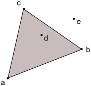
Fig. 1: Convex set.

Example 3.

Now, we introduce a further scaling method, the so-called hierarchical nominal scaling. This scaling method is inspired by the occupations of persons within a social survey. Usually occupations are categorised within a hierarchy of different levels. On a first level occupations are split into different categories $(a_{1},b_{1},...)$. For example category $a_{1}$ could be “Managers”, category $b_{1}$ “Professionals”, etc. Each of these categories is then split again on a more fine-grained level (Level 2) into further subcategories. In this case, category $a_{1}$ is split into $a_{1}a_{2}$ “Managers: Chief executives, senior officials, and legislators” and $a_{1}b_{2}$ “Managers: Administrative and commercial managers” and so on. Note that the Level 2 subcategories based on the first level $b_{1}$ split do not have to match those of the Level 2 splits based on the Level 1 $a_{1}$ split. Subsequently, the Level 2 categories are again subdivided into subcategories, and so on. Such data structure can be conceptually scaled naturally. For every level, we introduce attributes describing every single category based on the upper level classification, see Table 2. Here, for simplicity, we used only two levels with two categories, respectively.

	$a_{1}$	$b_{1}$	$a_{1}a_{2}$	$a_{1}b_{2}$	$b_{1}a_{2}$	$b_{1}b_{2}$
$a_{1}a_{2}$	x		x
$a_{1}b_{2}$	x			x
$b_{1}a_{2}$		x			x
$b_{1}b_{2}$		x				x

Table 2: Minimal example of a hierarchical nominal scaling with two levels ($1$, $2$) and two categories ($a$,$b$, respectively).

Now, let us take a closer look at the extents given by Table 2 which are

$$\{\emptyset,\{a_{1}a_{2}\},\{a_{1}b_{2}\},\{b_{1}a_{2}\},\{b_{1}b_{2}\},\{a_{1}a_{2},a_{1}b_{2}\},\{b_{1}a_{2},b_{1}b_{2}\},G\}.$$

Furthermore, we obtain that $a_{1}a_{2}\in\gamma(\{a_{1}b_{2},b_{1}a_{2}\})$.

Example 4.

In the next sections, we want to transfer the idea of depth functions from $\mathbb{R}^{d}$ to general non-standard data which are represented by a formal context. Before looking at this, we now discuss the reverse and show how one can represent the elements in $\mathbb{R}^{d}$ as objects of a formal context. We consider $\mathbb{R}^{d}$ together with the topology induced by the Euclidean norm. The scaling method introduced here is inspired by [20, 19]. Let $G=\mathbb{R}^{d}$ be the object set and the attribute set $M=\{H\subseteq\mathbb{R}^{d}\mid H\text{ topologically closed halfspace}\}$ is the set of all topologically closed halfspaces. We say that there exists a relation $(g,H)\in I$ between an object/point $g\in G=\mathbb{R}^{d}$ and an attribute/halfspace $H\in M$ if and only if $g\in H$. Then $\mathbb{K}_{\mathbb{R}^{d}}=(G,M,I)$ gives us a formal context.

In the next step, let us consider the set $\gamma(2^{G})$ with $\gamma$ being induced by the formal context $\mathbb{K}_{\mathbb{R}^{d}}$. Let $A\subseteq G=\mathbb{R}^{d}$. Then $\Psi(A)$ are all halfspaces which contain every object/point in $A$. Further on, $\gamma(A)=\Phi\circ\Psi(A)$ are then every object/point which lies in every halfspace in $\Psi(A)$. Thus $\gamma(A)$ is the intersection of all halfspaces in $\Psi(A)$ and therefore a topologically closed convex set. More generally, one can show that for every topologically closed convex set in $2^{\mathbb{R}^{d}}$ there exists a set $A\subseteq G=\mathbb{R}^{d}$ such that this convex set is given by $\gamma(A)$. Thus, $\gamma$ is the convex closure operator on $\mathbb{R}^{d}$ and the extent set $\gamma(2^{G})$ is the set of all topologically closed convex sets.

More concretely, assume that $d=2$ and consider Figure 1. Then $d\in\gamma(\{a,b,c\})$. This means that $d$ lies in every topologically closed halfspace which contains also $a,\>b$, and $c$. In other words, $d$ shares the same attributes as $a,b,c$ share. Thus, one can say that $d$ is implied by $a,b$ and $c$ based on $\gamma$. Since $e\not\in\gamma(\{a,b,c\})$, there exists a halfspace which contains $a,b$ and $c$ but not $e$. This shows how the concrete definition of the closure system enhances the connection between single objects.

3 Definition of depth functions for non-standard data using formal concept analysis

Our aim in this section is to give a general definition of data depth functions for non-standard data types using formal concept analysis. By representing the data points $G$ via a formal context, with $G$ being the object set, we obtain a unified structure that is not tailored to one specific data type. In particular, the newly provided depth function allows to analyse a large variety of different data types on centrality and oultyingness issues. With this, nonparametric methods can be developed for all these data.

The depth function presented here only specifies the domain and codomain but not the exact mapping rule. Thus, the structural properties presented later, see Section 4, can be seen as generic properties for this kind of depth functions.

Definition 4.

We define a depth function using formal concept analysis by

$$D_{G}:G\times\varkappa_{G}\times\mathscr{P}_{G}\to\mathbb{R}_{\geq 0}$$

for a fixed set of objects $G$ and a set of formal contexts $\varkappa_{G}\subseteq\{\mathbb{K}\mid G\text{ is object set of }\mathbb{K}\}$. $\mathscr{P}_{G}$ is a set of probability measures on $G$ defined on a $\sigma$-field which contains all extent sets of the corresponding formal contexts of $\varkappa_{G}$ .

Thus, we compute the depth of an object set based on a probability measure and formal context representing the object relationships. We want to emphasise that $G$, $\varkappa_{G}$ and $\mathscr{P}_{G}$ mutually depend on each other. Sometimes the restriction of $\varkappa_{G}$ and $\mathscr{P}_{G}$ to a subset of all possible formal contexts or probability measures is necessary. For example, assume that $G=[0,1]$, then for every subset of $G$ there exists a formal context such that this subset is an extent. Thus, in this case, a restriction to a subset of contexts is necessary if we want to allow the uniform distribution to be an element of $\mathscr{P}_{G}$. This follows from [21, Chapter 1.1] which shows that there cannot exist a probability measure on $[0,1]$ which formalises the intuition of volume and has the entire power set of $[0,1]$ as input. Another aspect is that restriction can lead to a set of formal contexts fulfilling additional structural requirements. With this, it can be possible to define mapping rules which are not possible in general. (See Section 4, Property (P8) does not hold for every formal context, but only for a subset.) Another example is given in [1] and [2] where we considered one single formal context on the set of partial orders. There, we used the structure given by this concrete formal context to define the mapping rule. The same reasoning can be applied to the probability set $\mathscr{P}_{G}$. Thus, for a proper definition of the depth function, not only the exact mapping rule is important, but the considered formal contexts and probability measures as well.

A data set can be represented by different attribute sets and corresponding binary relations. Thus, Definition 4 can lead to many different depth functions even if the object set $G$, the probability $\Pr\in\mathscr{P}_{G}$, and a concrete mapping rule are specified. Hence, the choice of formal context and scaling method can have a huge impact on the depth values, i.e. this can also be seen in Section 4.

The empirical depth function corresponds to the depth function in Definition 4 with the empirical probability measure as input. To ensure that the empirical depth function is well defined we need to assume that every empirical probability measure $\Pr_{G}^{(n)}$ of every probability measure $\Pr_{G}\in\mathscr{P}_{G}$ is again an element of $\mathscr{P}_{G}$.

Definition 5.

Let $G$ be a set and $\varkappa_{G}\subseteq\{\mathbb{K}\mid G\text{ is object set of }\mathbb{K}\}$ a set of formal contexts on $G$. We assume that $\mathscr{P}_{G}$ consists of probability measures that are defined upon a $\sigma$-field containing all extents of $\varkappa_{G}$. Furthermore, we assume that for every sample $g_{1},\ldots,g_{n}$ based on a probability measure $\Pr_{G}\in\mathscr{P}_{G}$, we get for the empirical probability measure $\text{Pr}^{(n)}_{G}$ that $\text{Pr}^{(n)}_{G}\in\mathscr{P}_{G}$ is true. Then the empirical depth function for a sample $g_{1},\ldots,g_{n}$ with corresponding empirical probability measure $\text{Pr}^{(n)}_{G}$ is given by

$$D_{G}^{(n)}:G\times\varkappa_{G}\to\mathbb{R}_{\geq 0},(g,\mathbb{K})\mapsto D_{G}(g,\mathbb{K},\text{Pr}^{(n)}_{G}).$$

Serving as an example, we consider the generalised Tukey depth, based on [19, 20] and introduced in [1]. The Tukey depth on $\mathbb{R}^{d}$ of a point $g\in\mathbb{R}^{d}$, compare to [22, 5], is the smallest probability of a halfspace containing $g$. To build the bridge to formal concept analysis, we consider the formal context $\mathbb{K}$ with the object set $G=\mathbb{R}^{d}$, attribute set $M=\{H\subseteq\mathbb{R}^{d}\mid H\text{ topologically closed halfspace}\}$ and binary relation $I$ with $(g,H)\in I$ if and only if $g\in H$, see Example 4. Based on this the Tukey depth for a point $g\in\mathbb{R}^{d}$ and probability measure $\Pr_{\mathbb{R}^{d}}$ on $\mathbb{R}^{d}$ can be written as

$$\inf_{H\in\mathcal{H}(g)}\text{Pr}_{\mathbb{R}^{d}}(H)=\inf_{H\in\Psi(g)}\text{Pr}_{\mathbb{R}^{d}}(H)=1-\sup_{H\in\Psi(g)}\text{Pr}_{\mathbb{R}^{d}}(G\setminus H)=1-\sup_{H\in M\setminus\Psi(g)}\text{Pr}_{\mathbb{R}^{d}}(H)=1-\sup_{m\in M\setminus\Psi(g)}\text{Pr}_{\mathbb{R}^{d}}(\Phi(m))$$ (1)

where $\mathcal{H}(g)$ is the set of all topologically closed halfspaces containing $g$ and $\Phi,\Psi$ correspond to the derivation operators given by the formal context $\mathbb{K}_{\mathbb{R}^{d}}$, see Section 2. The first equality translates the term to formal concept analysis terminology. The third equality holds because $G\setminus H$ is a topologically open halfspace and the supremum does not change when considering topologically closed halfspaces instead. The last equality is again a further translation into formal concept analysis that does not rely on the notion of a halfspace.

The right hand side of Equation (1) will now be the basis of the generalisation of Tukey depth to arbitrary formal contexts. Before we proceed, we shortly indicate, why we do not use directly the left hand side of Equation (1): Generally, the topologically closed convex sets in $\mathbb{R}^{d}$ correspond to the extents within our approach to use formal concept analysis to define data depth functions. On the other hand, the topologically closed halfspaces of $\mathbb{R}^{d}$ have no general natural equivalent in formal concept analysis. On the left hand side, if we replace the family of topologically closed halfspaces with the family of all extents, we obtain a depth value of zero for all $g\in\mathbb{R}^{d}$ when, e.g., the probability measure is continuous w.r.t. the Lebesgue measure. This is of course unsatisfying. Moreover, note that unlike halfspaces, the complement of extents in formal concept analysis are generally not extents. This further separates the left and the right hand side of Equation (1). Therefore, we take the right hand side of Equation (1). As will be shown later, see Section 5, if we take the supremum over all halfspaces or if we take the supremum over all topologically closed convex sets in $\mathbb{R}^{d}$ does not change the result. This can also be applied to the case of the generalised Tukey depth.

Additionally, the supremum of the right hand side of Equation (1) has a natural interpretation as a measure of oulyingness that can be expressed in the language of formal concept analysis, see [19, Section 2] and [20, Section 5]. In these articles, the author constructs special representative extents: One can say that an extent is very general if it contains at least a certain amount $\alpha$ of data points or probability mass. Of course, for given $\alpha$ there are many such extents but one can take for one $\alpha$ the intersection of all these extents. This intersection is again an extent which is then in a certain sense a representative extent w.r.t. a level $\alpha$. The outlyingness of a point $g$ is then given by the (empirical) probability mass of the most specific depth contour (i.e., the most specific representative extent that corresponds to the smallest possible $\alpha$) that still contains $g$. A slightly different, but order-theoretically equivalent, definition is to take the least specific depth contour that does not contain $g$. This is exactly what is done by $\sup_{m\in M\setminus\Psi(g)}\text{Pr}_{\mathbb{R}^{d}}(\Phi(m))$ in Equation (1). With this motivation, we get as generalised Tukey depth:

Definition 6.

Let $G$ be a set, $\varkappa_{G}$ a subset of formal contexts and $\mathscr{P}_{G}$ a subset of probability measures on $G$. Assume that $\varkappa_{G}$ and $\mathscr{P}_{G}$ are defined as in Definition 4. The generalised Tukey depth is given by

$$T_{G}:\begin{array}[]{l}G\times\varkappa_{G}\times\mathscr{P}_{G}\to[0,1],\\ (g,\mathbb{K},\Pr_{G})\mapsto 1-\sup_{m\in M\setminus\Psi(g)}\Pr_{G}(\Phi(m))\end{array}$$

where $\mathbb{K}$ defines the operator $\Phi$ and $\Psi$. We set $\sup_{t\in\emptyset}f(t)\mathrel{\hbox to0.0pt{\raisebox{1.29167pt}{$\cdot$}\hss}\raisebox{-1.29167pt}{$\cdot$}}=0$ for every function $f$.

Note that $\varkappa_{G}$ is not restricted to any subset and, in particular, $\Pr_{G}$ is only restricted by $\varkappa_{G}$, see Definition 4. The second part of the mapping rule in Definition 6, $\sup_{m\in M\setminus\Psi(g)}\Pr_{G}(\Phi(m))$, corresponds to the supremum of the probabilities of the events which consists of all objects having an attribute the object of interest does not have. Thus, if $g\in G$ is an object that has all the attributes which occur, then $g$ has a maximal depth of value one.

Now, we define the empirical version. Analogously to Definition 5, let $g_{1},\ldots,g_{n}$ be a sample of $G$ based on $\Pr_{G}\in\mathscr{P}_{G}$. Then the empirical Tukey depth function corresponds to $T_{G}$ by inserting the corresponding empirical probability measure $\Pr_{G}^{(n)}$. This gives us:

Definition 7.

Let $G$, $\varkappa_{G}$ and $\mathscr{P}_{G}$ be defined as in Definition 5. Then the empirical generalised Tukey depth is

$$T^{(n)}_{G}:\begin{array}[]{l}G\times\varkappa_{G}\to\mathbb{R}_{\geq 0},\\ (g,\mathbb{K})\mapsto 1-\sup_{m\in M\setminus\Psi(g)}\sum_{\tilde{g}\in\Phi(m)}\text{Pr}_{G}^{(n)}(\tilde{g}).\end{array}$$

Example 5.

Recall Example 1 and 2. Let us assume that the probability measure $\Pr_{G}$ on $G=\{p_{1},p_{2},p_{3}\}$ is given by $\Pr_{G}(p_{1})=\Pr_{G}(p_{2})=1/4$ and $\Pr_{G}(p_{3})=1/2$. Then the generalised Tukey depth of $p_{1}$ and $p_{3}$ are

$$T^{(n)}_{G}(p_{1})=1-\sup_{m\in M\setminus\Psi(p_{1})}\text{Pr}_{G}(\Phi(m))=1-\sup_{m\in\{\text{``$\geq 0.7$ ''},\text{``$\geq 0.5$ ''},b,c\}}\text{Pr}_{G}(\Phi(m))=\frac{1}{4},$$

$$T^{(n)}_{G}(p_{3})=1-\sup_{m\in M\setminus\Psi(p_{3})}\text{Pr}_{G}(\Phi(m))=1-\sup_{m\in\{\text{``$\leq 0$ ''},\text{``$\leq 0.5$ ''},b,c\}}\text{Pr}_{G}(\Phi(m))=\frac{1}{2}.$$

Before presenting the structural properties, we define when two depth functions are isomorph and thus represent the same center-outward order.

Definition 8.

Let $G$ be a set and $D_{G}$ and $\tilde{D}_{G}$ be two depth functions based on $\varkappa_{G}$ and $\mathscr{P}_{G}$, $\tilde{\varkappa_{G}}$ and $\tilde{\mathscr{P}}_{G}$ respectively, see Definition 4. Let $\mathbb{K}\in\varkappa_{G}$, $\tilde{\mathbb{K}}\in\tilde{\varkappa}_{G}$, $\Pr_{G}\in\mathscr{P}_{G}$ and $\tilde{\Pr}\in\tilde{\mathscr{P}}_{G}$. Then $D_{G}(\cdot,\mathbb{K},\Pr_{G})$ and $\tilde{D}_{G}(\cdot,\tilde{\mathbb{K}},\tilde{\Pr}_{G})$ on $G$ are isomorph if and only if there exists a bijective and bimeasureable function $i:G\to G$ such that

$$D_{G}(g,\mathbb{K},\text{Pr}_{G})\leq D_{G}(\tilde{g},\mathbb{K},\text{Pr}_{G})\Longleftrightarrow\tilde{D}_{G}(i(g),\tilde{\mathbb{K}},\tilde{\Pr}_{G})\leq\tilde{D}_{G}(i(\tilde{g}),\tilde{\mathbb{K}},\tilde{\Pr}_{G})$$

is true for all $g,\tilde{g}\in G$. In what follows, $\cong$ denotes the isomorphism between two depth functions.

For simplicity of notation, we write $D$, $D^{(n)}$, $T$, $T^{(n)}$, $\varkappa$, $\mathscr{P}$, $\Pr$ and $\Pr^{(n)}$ instead of $D_{G}$, $D_{G}^{(n)}$, $T_{G}$, $T_{G}^{(n)}$, $\varkappa_{G}$, $\mathscr{P}_{G}$, $\Pr_{G}$ and $\Pr_{G}^{(n)}$ in the following if the underlying object set $G$ is clear.

4 Structural properties characterising the depth function using formal concept analysis

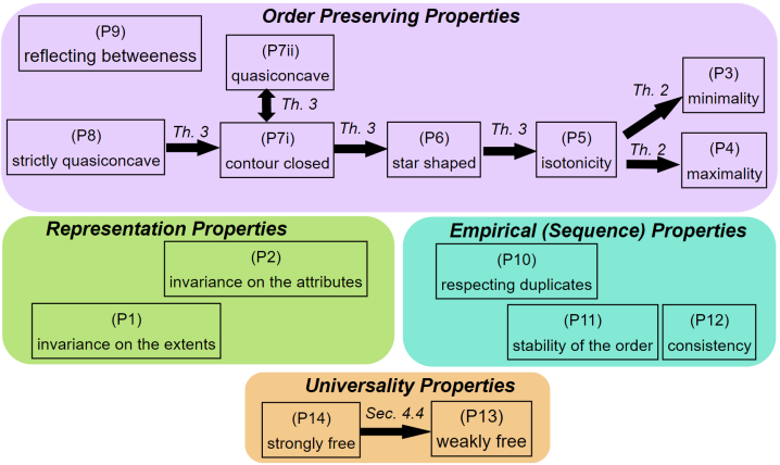
Fig. 2: Overview of the structural properties together with their mathematical connections. Th is Theorem and Sec is Section for short. This overview contains all direct implications between the properties. Further connections like, e.g., that Properties (P8) and (P9) imply one concrete center-outward order in special cases, see, e.g., Theorem 5, or under which assumptions certain properties are never or always true, see, e.g., Theorem 6, are not presented in the Figure.

After this general definition of depth functions based on formal concept analysis, we want to discuss some structural properties a depth function can have. With this, we tackle the question of what centrality is and which object is - in some sense - closer to the center than another object. In particular, we provide concepts to discuss centrality and outlyingness for different data types without necessarily presupposing one specific data structure. Thus, this section gives a starting point for a discussion on centrality, outlyingness, and depth functions based on formal concept analysis. Furthermore, we define a framework upon which newly introduced depth functions can be studied and compared.

For normed vector spaces, there is already an ongoing discussion about this. The authors of [14, 23, 15, 16] are concerned about these questions for data depth functions defined on $\mathbb{R}^{d}$. Furthermore, [11, 7] discuss depth functions and centrality topics for functional data. All these examples have in common that they are based on a normed vector space and that the clarification of centrality and outlyingness is done by defining properties. For example, [23, 15] demand that the depth of a point $x\in\mathbb{R}^{d}$ should converge to zero as the norm of $x$, i.e. $||x||$, tends to infinity. This reflects the intuition about outlyingness in unbounded spaces. In contrast to outlyingness, the definition of a center point does not immediately follow. Basically, every point in $\mathbb{R}^{d}$ can be the center. This follows from the fact that after translation, rotation, etc. the structure of a normed vector space does not change. The center generally seems to be only naturally specified in special cases. For example [23] assumes that for a probability measure that is symmetric around a point $c$, see [24], this point $c$ should then be the center. In the case of a multivariate normal distribution, the center point is the mean vector. Since a depth function should represent a center-outward order, this point $c$ needs to have a maximal depth value. Together with the center, one needs to discuss what it means that one point is further away from the center than another. In $\mathbb{R}^{d}$, this is achieved by the use of line segments, see [23, 15]. A point $p_{1}$ which lies on the line segment between the center and a further point $p_{2}$ is said to be closer to the center than $p_{2}$. In other words, $p_{2}$ is more outlying than $p_{1}$. At the first glance, here we also use the normed vector space structure.

It follows from the above that the definition of the terms centrality and outlyingness seem to highly rely on the underlying distribution. In particular, the part defining the center point which is based on a symmetric distribution, see [24]. Slightly different to [23, 24] is the approach of [15]. Here the notion of a depth function is based more directly on the structure of the normed vector space. The properties given by [15] put emphasis on the structure of the underlying spaces and not on the probability measure. Thus, in contrast to e.g., [23, 24], the definition of centrality of a point is more detached from the notion of a point of symmetry/centrality of the underlying probability measure. Note that [15] gives an even stronger definition of depth functions. In the following, we discuss the term centrality and outlyingness from the perspective of the approach in [15].

In this article, we consider a space $G$ where the structure of the data points is given by a formal context. In the style of [23] and [15] for depth functions in $\mathbb{R}^{d}$, we define structural properties of a depth function based on formal concept analysis to clarify the notion of centrality and outlyingness. These properties express characteristics of the data set when represented via a formal context and how these characteristics are included in the depth function. Some of the structural properties build upon the existing ones in $\mathbb{R}^{d}$ that we transfer to our new situation. To achieve this, we use that the set of all topologically closed convex sets is a natural closure system on $\mathbb{R}^{d}$. Since the extent set also defines a closure system, we obtain a direct translation to formal concept analysis by representing the properties by use of the convex closure system on $\mathbb{R}^{d}$. For example, we transfer the idea of a line segment to our data representation via a formal context, see Property (P6). Moreover, the “quasiconcavity” property, see [15, p. 19] has a natural translation to formal concept analysis by use of the closure system, see Property (P7i and ii). Other introduced structural properties use formal concept analysis directly. An example is the maximality property (P4). Here, we say that an object which lies in every set of the closure system needs to have maximal depth value. While in $\mathbb{R}^{d}$ the closure system and the translated closure system are equal, this cannot be said in general for all closure systems. In particular, the concept of translation cannot be properly defined for every space $G$. Instead, we use that in some cases the data itself contains natural center or outward lying points, see Properties (P3) and (P4) later. All in all, one can say that the introduced structural properties are defined and discussed within two perspectives: Transferring already existing properties in $\mathbb{R}^{d}$ and new development of properties based on the theory of formal concept analysis.

In total 14 structural properties are presented which can be covered under four different categories: Representation properties, order preserving properties, empirical (sequence) properties, and universality properties. An overview of the structural properties together with their mathematical connections can be seen in Figure 2. In what follows, we fix the set of objects $G$ and consider the depth function $D:G\times\varkappa\times\mathscr{P}\to\mathbb{R}_{\geq 0}$. Furthermore, we refer to Definition 4 when we say that $D$ is a depth function. We use the term empirical depth function when considering a depth function in the style of Definition 5. Afterwards, in Section 5 we check these properties based on the introduced generalised Tukey depth, see Section 3.

4.1 Representation properties

Depth functions satisfying the following properties are structure preserving on $G$. This includes two parts: First, assume that we represent the data set by two formal contexts and that we consider two probability measures. Let us assume that between the corresponding extent sets and therefore the structure of the objects exists a bijective function. Furthermore, if additionally the probability values are preserved by this bijective function, then the depth function should be preserved as well. In other words, the order given by the depth function should not rely on the used scaling method unless it does substantially change the structure of the extent sets. Also, the influence of the probability measure is only based on the extent sets. This can be seen as an adaptation of the “affine invariance” property of depth functions in $\mathbb{R}^{d}$, see [23, p. 463]. There, the depth function equals the depth of the shifted version if the probability measure is shifted accordingly.

The second part of the representation properties considers the attribute values. Here, we say that the depth function preserves the structure if and only if two objects with the same attributes have the same depth value. From the perspective of formal concept analysis, two objects with the same attributes are duplicates and therefore they should be assigned to the same depth value.

1. Invariance on the extents: Let $\mathbb{K},\tilde{\mathbb{K}}\in\varkappa$ be two formal contexts on $G$ and let $\Pr,\tilde{\Pr}\in\mathscr{P}$ be two probability measures on $G$. If there exists a bijective and bimeasureable function $i:G\to G$ such that the extents are preserved (i.e. $E$ extent w.r.t. $\mathbb{K}$ $\Leftrightarrow i(E)$ extent w.r.t. $\tilde{\mathbb{K}}$) and the probability is also preserved (i.e. $\Pr(E)=\tilde{\Pr}(i(E))$), then

   $$D(\cdot,\mathbb{K},\Pr)\cong D(\cdot,\tilde{\mathbb{K}},\tilde{\Pr})$$

   is true.

1. Invariance on the attributes: For every $\mathbb{K}\in\varkappa$, $\Pr\in\mathscr{P}$ and $g_{1},g_{2}\in G$ with $\Psi_{\mathbb{K}}(\{g_{1}\})=\Psi_{\mathbb{K}}(\{g_{2}\})$,

   $$D(g_{1},\mathbb{K},\Pr)=D(g_{2},\mathbb{K},\Pr)$$

   holds.

4.2 Order preserving properties

While the representation properties ensure that similar structures on $G$ lead to the same depth function, the next order preserving properties consider the obtained order by the depth function. Ignoring the last property in this section, these properties increase in their strength of restriction.

These properties are defined along the lines of “monotonicity relative to the deepest point” and “maximality at the center” properties, see [23, p. 463], and the “quasiconcavity” properties, see [15, p. 19], defined for $\mathbb{R}^{d}$. In contrast to $\mathbb{R}^{d}$ we neither have a norm nor a concept of translation and symmetry, but we can make use of the closure system and closure operator given by the extent set. When considering the properties defined for $\mathbb{R}^{d}$ in the context of the convex sets which define a closure system together with the corresponding closure operator, we can build a bridge to formal concept analysis. In particular, the “quasiconcavity” property, see [15, p. 19], has therefore a natural adaptation. Nevertheless, the convex sets are a special case of closure sets: For example, the affine invariance is reflected in the set since by shifting the set of convex sets the family of sets does not change. This does not hold in general for closure systems. For example, there exist closure systems where one point occurs more often in the sets of the closure system than another point. Another aspect is that we do not necessarily have infinitely many objects/data points which is needed for the “vanishing at infinity” property for $\mathbb{R}^{d}$, see [23, p. 464], where we say that the depth converges to zero for the norm of a point converging to infinity. Thus, this property cannot be transferred to our new situation. Instead, we use the concept of a formal context where two natural extreme opposite characteristics of the objects can occur. The first one: If an object has every attribute then it lies in every extent set. Conversely, if an object has no attribute at all, then the only extent containing this object is the entire set $G$. Property (P3) and (P4) now ensure that these two opposite characteristics are also reflected in the depth function.

1. Minimality: Let $\mathbb{K}\in\varkappa,\Pr\in\mathscr{P}$. Further, let $g_{non}\in G$ such that for every extent $E\subsetneq G$ of $\mathbb{K}$ we have that $g_{non}\not\in E$, then

   $$D(g_{non},\mathbb{K},\Pr)=\min_{g\in G}D(g,\mathbb{K},\Pr)$$

   is true.

2. Maximality: Let $\mathbb{K}\in\varkappa,\Pr\in\mathscr{P}$. Assume there exists $g_{all}\in G$ such that for every extent $E$ of $\mathbb{K}$ we have that $g_{all}\in E$. Then

   $$D(g_{all},\mathbb{K},\Pr)=\max_{g\in G}D(g,\mathbb{K},\Pr)$$

   holds.

Note that a depth function which fulfils these two properties does not rely on the probability measure to set the values of the two extreme cases. On the other hand, there exist formal contexts such that the objects $g_{non}$ or $g_{all}$ do not exist at all. Recall Example 4 where we considered the spatial data.

Nevertheless, since we have now predefined the maximal depth value in specific cases, this has to be in line with adapting properties like “monotone on rays” or “quasiconcavity”, see [15, p. 19]. In what follows we start with less restricting properties and increase their restriction strength slowly. We show that they imply Properties (P4) and (P3).

Property (P5) is inspired by the fact that in formal concept analysis, an object $g_{1}$ which lies in the closure of an other object $g_{2}$ implies that this object is more specific than $g_{2}$. In other words, $g_{2}$ has all attributes and possibly even more attributes than $g_{1}$. This is analogous to the assumption that $\gamma(\{g_{1}\})\supseteq\gamma(\{g_{2}\})$ is true. Thus, Property (P5) says that an object $g_{2}$ must have a depth value as least as high as $g_{1}$.

1. Isotonicity: For every $\Pr\in\mathscr{P}$ and formal context $\mathbb{K}\in\varkappa$ with $g_{1},g_{2}\in G$ such that $\gamma_{\mathbb{K}}(\{g_{1}\})\supseteq\gamma_{\mathbb{K}}(\{g_{2}\})$,

   $$D(g_{1},\mathbb{K},\Pr)\leq D(g_{2},\mathbb{K},\Pr)$$

   is fulfilled.

There exists a natural strengthening of the isotonicity property (P5) which leads to the adaptation of the “monotonicity relative to deepest point”, see [23, p. 463] property in $\mathbb{R}^{d}$. For start, let us assume that the depth function is bounded from above. Furthermore, we assume that the depth function has its maximum at center $c\in G$. The “monotone on rays” in $\mathbb{R}^{d}$ definition in [15, p. 19] states that the depth of a point that moves further away from the center $c$ on a fixed ray should decrease. Since we do neither have a norm nor a vector space, we cannot generally define what further away as well as ray means. Thus, we translate the definition to a setting using the convex closure operator instead. In this case, if a point/object $\tilde{g}$ lies on the line segment given by a further point $g$ and the center $c$, then the depth of $\tilde{g}$ must be at least as high as the depth of $g$. In other words, when a point $\tilde{g}$ lies in the convex closure of another point $g$ and the center, then we have a lower bound for the depth of $\tilde{g}$. Thus, the points/objects with depth values larger or equal to a fixed value form a starshaped set. This gives the name of the property. With the definition based on the convex closure system, we can easily transfer this property to formal concept analysis and obtain Property (P6).

1. Starshapedness: Let $\mathbb{K}\in\varkappa$ and $\Pr\in\mathscr{P}$. If there exists at least one center point $c\in G$ such that for all $g\in G$ and all $\tilde{g}\in\gamma_{\mathbb{K}}(\{c,g\})$ we have

   $$D(\tilde{g},\mathbb{K},\Pr)\geq D(g,\mathbb{K},\Pr),$$

   then we call $D$ starshaped.

In the above explanation, we assumed that the center point $c$ has a maximal depth value. This assumption is not included in the definition of Property (P6) as the boundedness of the depth function, as well as the maximality at the center, follow directly. Let us fix $c\in G$ to be one center point. Since for every closure operator the isotonicity assumption (see Section 2, not to be confused with Property (P5)) holds, we get that for every object $g$ we have $c\in\gamma(\{c,g\})$. Thus, by Property (P6) for every $g\in G$ we obtain

$$D(c,\mathbb{K},\Pr)\geq D(g,\mathbb{K},\Pr).$$

With this, $c$ must have the highest depth value. Since the depth function maps to $\mathbb{R}$, this gives us also the upper bound of the depth function.

Furthermore, the starshaped property (P6) together with the invariance on the extents property (P1) has some implications on the point of maximal depth when the underlying probability measure has some symmetry property. As already indicated at the beginning of Section 4, because of the lack of a translation operation, etc., it is difficult to define symmetry in our setting. However, one can still define some notion of point symmetry, see the next theorem.

Theorem 1.

Let $\mathbb{K}\in\varkappa$ and $\Pr\in\mathscr{P}$ (both based on set $G$). We assume that $\Pr$ is point symmetric around $s\in G$ in the following sense: There exists a bimeasurable involutory function $i:G\longrightarrow G$ such that

1. $\Pr(i(E))=\Pr(E)$ for all extents $E\subseteq G$ and

2. for all $g\in G$ we have $s\in\gamma(\{g,i(g)\})$.

Then for every depth function which fulfils Properties (P1) and (P6), the center of symmetry $s$ of $\Pr$ has maximal depth.

Proof.

Let $c$ be one center point. First note that by Assumption 2. we get $s\in\gamma(\{c,i(c)\})$. Because $D$ is starshaped, we have $D(s,\mathbb{K},\Pr)\geq D(i(c),\mathbb{K},\Pr)$. Now, we use that there exists a bimeasurable involutory function $i$ and that $D$ is invariant on the extents (P1) to get $D(i(c),\mathbb{K},\Pr)=D(c,\mathbb{K},\Pr)$. With this, we conclude that $D(s,\mathbb{K},\Pr)\geq D(c,\mathbb{K},Pr)$. This proves that $s$ has maximal depth. ∎

Note that object $s$ of Theorem 1 is not necessarily a center point in the style of Property (P6).

These properties are written down in their order of strength. More precisely, Property (P6) implies Property (P5) and Property (P5) implies Properties (P4) and (P3), see Theorem 2. Thus, if Property (P6) is satisfied and if there exists an object $g$ which has every attribute, then $c$ must be one of the center point $c$ discussed in Property (P6).

Theorem 2.

Let $\mathbb{K}\in\varkappa$ and $\Pr\in\mathscr{P}$. Let $D$ be a depth function then the following implications hold for $D$:

1. Let $c\in G$ be a center object. If $D$ satisfies Property (P6), then Property (P5) is true for $D$.

2. If $D$ satisfies Property (P5), then Properties (P4) and (P3) are true for $D$.

Proof.

Assume that $\mathbb{K}\in\varkappa$ and $\Pr\in\mathscr{P}$. Let $D$ be a depth function.

We begin by proving that Property (P6) implies Property (P5). Therefore assume that Property (P6) is true for $D$ and let $c\in G$ be one center point. Further let $g_{1},g_{2}\in G$ such that $\gamma_{\mathbb{K}}(\{g_{1}\})\supseteq\gamma_{\mathbb{K}}(\{g_{2}\})$. Then we get that $g_{2}\in\gamma(\{c,g_{1}\})$ and therefore we have $D(g_{1},\mathbb{K},\Pr)\leq D(g_{2},\mathbb{K},\Pr)$.

The next step is to show that Property (P5) implies Property (P4). Assume that Property (P5) is satisfied and that $g_{all}$ lies in every extent set. Then, we get for every $g\in G$ that $\gamma_{\mathbb{K}}(\{g_{all}\})\supseteq\gamma_{\mathbb{K}}(\{g\})$ holds. Thus, $D(g_{all},\mathbb{K},\Pr)\geq\max_{\{g\in G\}\}}D(g,\mathbb{K},\Pr)$ is true and Property (P4) follows.

Finally, we show that Property (P3) follows from Property (P5). Let $g_{non}\in G$ be an object which lies only in the entire set and in no other extent set. Furthermore, we suppose that Property (P5) is true for $D$. Since $\gamma(\{g_{non}\})=G$ for every $g\in G$ we have $\gamma(\{g\})\subseteq\gamma(\{g_{non}\})$. Due to Property (P5) we follow that $D(g_{non},\mathbb{K},\Pr)\leq D(g,\mathbb{K},\Pr)$ for every $g\in G$. This gives us Property (P3). ∎

Remark 1.

Let us point out some consequences of Property (P6). In contrast to [23, p. 463] we do not assume that the center $c$ is unique. For example, the depth function is allowed to have a plateau at the highest point. In particular, we allow the depth function to be constant. Especially $g_{non}$ can only be the center point if the function is constant, due to Properties (P3), (P4) and Theorem 2. Moreover, we get that when the depth function has at least two different values, then $g_{non}$ must have the minimal value and $g_{all}$ the maximal value. This allows us to specify a center point and an outlying point without relying on the other observed points/objects by defining the scaling method. Note that this situation does not occur often. For example, all scaling methods described in Section 2 do not have an object $g_{non}$ and $g_{all}$.

Nevertheless, this stresses the importance of a meaningful and carefully chosen scaling method. Observe that the difference between having an attribute and not having an attribute is not symmetric and cannot be switched without eventually fundamentally changing the characteristic of the corresponding closure system.

The next order preserving properties are in the style of the “quasiconcavity” property, see, e.g., [15, p. 19]. In the context of $\mathbb{R}^{d}$ quasiconcavity states that the set of all points with a larger (or equal) depth value than $\alpha\geq 0$ needs to be a convex set. These sets are called contour sets. In this case, there is a direct transfer to formal concept analysis by the extent set as a closure system. Therefore, we first have to define the contour sets within the theory of formal concept analysis. Let $\mathbb{K}\in\varkappa$ be a formal context and $\Pr\in\mathscr{P}$ be a probability measure. For $\alpha\in\text{im}(D(\cdot,\mathbb{K},\Pr))$ the contour set $Cont_{\alpha}$ is defined as follows

$$Cont_{\alpha}\mathrel{\hbox to0.0pt{\raisebox{1.29167pt}{$\cdot$}\hss}\raisebox{-1.29167pt}{$\cdot$}}=\{g\in G\mid D(g,\mathbb{K},\Pr)\geq\alpha\}.$$

Now, we say the depth function is quasiconcave if every contour set is an extent set. This is stated in Property (P7i). Instead of considering the contour sets, an analogous statement for Property (P7i) is given in Property (P7ii). Here, we assure that the depth of an observation that lies in the closure of an input set is larger or equal to the infimum of the input. Property (P7ii) has a natural strengthening by assuming strict inequalities instead, see Property (P8).

1. Countourclosed: For every formal context $\mathbb{K}\in\varkappa$, probability measure $\Pr\in\mathscr{P}$ and every $\alpha\in\text{im}(D(\cdot,\mathbb{K},\Pr))$ the contour set $Cont_{\alpha}$ is an extent of the context $\mathbb{K}\in\mathcal{C}$.

2. Quasiconcave: Let $\mathbb{K}\in\varkappa$ and $\Pr\in\mathscr{P}$. If for all $A\subseteq G$ and all $g\in\gamma_{\mathbb{K}}(A)\setminus A$ we have

   $$D(g,\mathbb{K},\Pr)\geq\inf_{\tilde{g}\in A}D(\tilde{g},\mathbb{K},\Pr),$$

   we call $D$ quasiconcave.

3. Strictly quasiconcave: Let $\mathbb{K}\in\varkappa$ and $\Pr\in\mathscr{P}$. If for all $A\subseteq G$ and all $g\in\gamma_{\mathbb{K}}(A)\setminus A$ we have

   $$D(g,\mathbb{K},\Pr)>\inf_{\tilde{g}\in A}D(\tilde{g},\mathbb{K},\Pr),$$

   $D$ is strictly quasiconcave.

Again these properties have mathematical connections to each other. First of all, Property (P7i) and (P7ii) are equivalent. Secondly, Property (P8) is indeed stronger and implies Property (P7 i and ii). Thirdly, if $c$ is a center point with maximal depth, then with this $c$ we can show that (P7i and ii) imply the starshaped property (P6). Moreover, Property (P7i) implies Property (P5).

Theorem 3.

Let $\mathbb{K}\in\varkappa$ be a formal context and $\Pr\in\mathscr{P}$ a probability measure. Let $D(\cdot,\mathbb{K},\Pr)$ be a depth function.

1. Statement (P7i) and (P7ii) are equivalent.

2. Property (P8) implies (P7ii).

3. If their exists $c\in G$ with maximal depth value, then Property (P7ii) implies (P6) with $c$ being a center object.

4. Property (P7ii) implies (P5).

Proof.

Let $\mathbb{K}\in\varkappa$ and $\Pr\in\mathscr{P}$. Let $D(\cdot,\mathbb{K},\Pr)$ a depth function. Note that the claim that Property (P8) implies (P7ii) is given immediately. Thus, we only show Part 1., 3. and 4. of Theorem 3.

1. First assume that Property (P7ii) is true and let $\alpha\in\text{im}(D(\cdot,\mathbb{K},\Pr))$ be arbitrary. We prove that Property (P7i) follows. Assume, by contradiction that $Cont_{\alpha}$ is not an extent set. Since $\gamma$ is a closure operator and therefore idempotent, there exists $g\in\gamma(Cont_{\alpha})\setminus Cont_{\alpha}$. Since Property (P7ii) is true, $D(g,\mathbb{K},\Pr)\geq\inf_{\tilde{g}\in Cont_{\alpha}}D(\tilde{g},\mathbb{K},\Pr)\geq\alpha$ holds. This contradicts $g\notin Cont_{\alpha}$ and we get that Property (P7i) is fulfilled.

   For the reverse let (P7i) be true and let $A\subseteq G$ be arbitrary. We set $\alpha=\inf_{\tilde{g}\in A}D(\tilde{g},\mathbb{K},\Pr)$ and we know that $A\subseteq Cont_{\alpha}$. By (P7i) we know that $Cont_{\alpha}$ is an extent set. Since $\gamma(A)$ is the smallest extent set containing $A$ and the set of extents is a closure system, we follow that $\gamma(A)\subseteq Cont_{\alpha}$. Thus the depth of every object $g\in\gamma(A)$ must be larger or equal to $\alpha$ which implies (P7ii).

2. Now, we assume that Property (P7ii) is true and we show that Property (P6) holds as well. Therefore, we assume that $c\in G$ has maximal depth value. Let $g,\tilde{g}\in G$ such that $\tilde{g}\in\gamma(\{c,g\})$ is true. Due to Property (P7ii) we get $D(\tilde{g},\mathbb{K},\Pr)\geq\min\{D(c,\mathbb{K},\Pr),D(g,\mathbb{K},\Pr)\}\geq D(g,\mathbb{K},\Pr).$ The last inequality follows from the assumption that $c$ has maximal depth value. This gives us Property (P6) with $c$ being one center object.

3. Finally, assume that Property (P7ii) holds. Let $g_{1},g_{2}\in G$ with $g_{1}\neq g_{2}$ such that $\gamma(g_{2})\supseteq\gamma(g_{1})$. Then the quasiconcavity property implies that $D(g_{1},\mathbb{K},\Pr)\geq D(g_{2},\mathbb{K},\Pr)$. This shows Property (P5).

∎

	$m_{1}$	$m_{2}$	$m_{3}$
$g_{1}$	$\times$
$g_{2}$		$\times$
$g_{3}$			$\times$

Table 3: Formal context: Cannot fulfil Property (P8).

Property (P8), the strictly quasiconcavity, is indeed a very strong assumption. In particular, there exist formal contexts such that Property (P8) can never be fulfilled. An example can be found in [1]. There, we discussed the special case of depth functions for partial orders and analysed Properties (P7i and ii) and (P8) in this case. We showed that the quasiconcavity cannot be fulfilled by the formal context of partial orders. Another example is given by Table 3. Here, let $G=\{g_{1},g_{2},g_{3}\}$ and let $\Pr$ be an arbitrary probability measure. In contradiction, let us assume that Property (P8) is true for a depth function $D$ on $G$. Since $\gamma(g_{1})=\{g_{1},g_{2},g_{3}\}=\gamma(g_{2})$ we get $D(g_{1},\mathbb{K},\Pr)<D(g_{2},\mathbb{K},\Pr)$ and $D(g_{2},\mathbb{K},\Pr)<D(g_{1},\mathbb{K},\Pr)$ must hold at once. Since this is not possible, Property (P8) cannot hold for this context. In contrast, the quasiconcavity property (P7ii) allows equality which solves such problems. Note that in the case of the formal context given by Table 3, Property (P7ii) leads to a constant depth function.

More generally, one can say that the strictly quasiconcavity assumption on $D$ can never be satisfied if one formal context $\mathbb{K}\in\varkappa$ is an element of the following set:

$$\mathscr{C}^{\cancel{P8}}=\left\{(G,M,I)\text{ formal context }\bigg{|}\begin{array}[]{l}\text{exist }A,\tilde{A}\subseteq G\text{ such that }\#A<\infty,\#\tilde{A}<\infty\text{ and }A\cap\tilde{A}=\emptyset\\ \text{and }A\subseteq\gamma(\tilde{A}),\>\tilde{A}\subseteq\gamma(A)\end{array}\right\}.$$

Theorem 4 proves that for every $\mathbb{K}\in\mathscr{C}^{\cancel{P8}}$ there exists no strictly quasiconcave depth function. Here, we get a contradiction with the strict larger assumption. This case occurs naturally when the scaling method assigns to two different objects the same attribute values.

Theorem 4.

For every $\mathbb{K}\in\mathscr{C}^{\cancel{P8}}$ and every $\Pr\in\mathscr{P}$ there exists no depth function $D$ such that Property (P8) is fulfilled.

Proof.

Let $\mathbb{K}\in\mathscr{C}^{\cancel{P8}}$. We assume that there exists a depth function $D$ and a probability measure $\Pr$ such that Property (P8) is satisfied. Since $A\subseteq\gamma(\tilde{A})$ and $\tilde{A}\subseteq\gamma(A)$ we get

$$\forall a\in A\setminus\tilde{A}\colon D(a,\mathbb{K},\Pr)>\inf_{\tilde{a}\in\tilde{A}}D(\tilde{a},\mathbb{K},\Pr)\qquad\text{and}\qquad\forall\tilde{a}\in\tilde{A}\setminus A\colon\inf_{a\in A}D(a,\mathbb{K},\Pr)<D(\tilde{a},\mathbb{K},\Pr).$$

Furthermore, we assumed that $\#A<\infty,\#\tilde{A}<\infty$ is true. Thus, the infimum is attained in $A$ and $\tilde{A}$. Let $a_{m}\in A$ be an argument of the minimum of $D(a,\mathbb{K},\Pr)$, and analogously we set $\tilde{a}_{m}\in\tilde{A}$. Since $A\cap\tilde{A}=\emptyset$, we obtain that $\tilde{a}_{m}\in\tilde{A}\setminus A$ and $a_{m}\not\in A\setminus\tilde{A}$. But with this we get

$$D(a_{m},\mathbb{K},\Pr)>D(\tilde{a}_{m},\mathbb{K},\Pr)\qquad\text{and}\qquad D(a_{m},\mathbb{K},\Pr)<D(\tilde{a}_{m},\mathbb{K},\Pr).$$

This cannot be true which contradicts the assumption of Property (P8) being true. ∎

We want to point out that $A$ and $\tilde{A}$ being finite is crucial since in the proof we used that the infimum is attained and not only the largest lower bound of the sets. Secondly, the intersection of $A$ and $\tilde{A}$ being empty is also necessary since else one can set the elements in the intersection to the minimal depth value. This is then following Property (P8).

While the importance of a meaningful scaling method for Properties (P3) and (P4) is easily seen, this comes also into account for the last properties. For example Property (P7ii) and (P8) state that the depth of an object $g$ which is implied by a set $A$, i.e. $g\in\gamma(A)$, must have larger (or equal) depth than the minimal depth value of the elements in $A$. In the context of formal concept analysis, one can say that $g$ contains all characteristics/similarities having the objects in $A$ in common or even more. Therefore it is at least as specific (or more) than all the elements in $A$ together. Thus, when defining the scaling method, not only the individual attribute values should be taken into account, but also which object combination is more specific than others.

The next property can be seen as the inverse property of Property (P8). It states that a strict inequality between depth values should be rooted in some sense in the structure of the underlying closure system which is given by the underlying formal context. More precisely, the idea behind Property (P9) is that if two objects $g$ and $\tilde{g}$ differ in their depth, then there exists a set that separates these two objects. Assume that $g$ has a strictly higher depth value than $\tilde{g}$. Then there exists a set $A$ with $g\not\in A$ and $g\in\gamma(A)$ such that every object in $A$ has higher or equal depth to $\tilde{g}$. Thus, the set $A$, which is not necessarily an extent set, divides the two objects. Note that $\tilde{g}$ can be in $A$.

1. Reflecting betweeness: Let $\mathbb{K}\in\varkappa$ and $\Pr\in\mathscr{P}$. If for $g,\tilde{g}\in G$ with $D(g,\mathbb{K},\Pr)>D(\tilde{g},\mathbb{K},\Pr)$ there exists a set $A\subseteq G$ with

   $$i)\quad \forall a\in A\colon D(a,\mathbb{K},\Pr)\geq D(\tilde{g},\mathbb{K},\Pr),$$

   $$ii)\quad g\in\gamma(A)\setminus A\>\text{ and }$$

   $$iii)\quad \tilde{g}\notin\gamma(A)\setminus A,$$

   then $D$ fulfils the reflecting betweeness property.

Note that Condition $iii)$ of Property (P9) can be easily fulfilled by adding $\tilde{g}$ to $A$. Property (P9) and (P8) together are very restrictive. Indeed when $G$ is finite and the formal context satisfies the meet distributivity assumption, then every depth function which fulfils both properties gives the same center-outward order structure of the objects. Thus, all depth functions are isomorph to each other. In particular, this order does not rely on the probability measure $\Pr$.

Definition 9.

Let $\mathbb{K}=(G,M,I)$ be a formal context. Let $E$ be an extent set of $\mathbb{K}$. We call an object $g\in G$ an extreme point of $E$ (given by $\mathbb{K}$) if and only if

$$g\in E\quad\text{ and }\quad g\not\in\>\gamma\left(E\setminus\{\tilde{g}\mid\Psi(\tilde{g})=\Psi(g)\}\right).$$

We denote the set of all extreme points of an extent $E$ by $\mathcal{E}_{E}$.

A formal context is meet distributive if and only if every extent is the closure of its extreme points.

An example for a meet distributive formal context is the spatial formal context given in Example 4 where $G$ is only a finite subset of $\mathbb{R}^{d}$. Here the extreme objects correspond to the extreme points of a convex set. Note that in the definition of the extreme points duplicates are deleted in the sense that duplication does not change the character of being an extreme point. Let us assume that the formal context $\mathbb{K}$ has no duplicates. Then we immediately obtain for every extent $E$ that there does not exist any further set $A\subseteq E$ with $A\cap\mathcal{E}_{E}\neq\mathcal{E}_{E}$ such that $\gamma(A)=E$. Thus, the extreme points are not only sufficient to imply $E$ but also necessary.

Theorem 5.

Let $G$ be finite and let $\mathbb{K}\in\varkappa$ be a meet distributive formal context with object set $G$. We assume that the context has no duplicates (i.e. $\not\exists g,\tilde{g}\in G$ with $g\neq\tilde{g}$ and $\Psi(g)=\Psi(\tilde{g})$). Let $D$ and $\tilde{D}$ be two depth functions on $G$ and $\mathbb{K}$ which fulfil Property (P8) and (P9). Then for every probability measure $\Pr\in\mathscr{P}$ the orders given by $D$ and $\tilde{D}$ are identical.

Proof.

We show this claim in two steps (see below):

• Step 1: Since Property (P7) is true, we conclude with the use of Property (P9) that all extreme points of $Cont_{\alpha}$ with $\alpha\in im(D(G,\mathbb{K},\Pr))$ must have the same depth value for some depth function $D$.

• Step 2: We use Property (P8), $G$ being finite and the extents are given by the extreme points to prove the claim.

Step 1: Let $D$ be a depth function which fulfils Properties (P8) and (P9). For every $\alpha\in im(D(G,\mathbb{K},\Pr))$ the extreme points $\mathcal{E}_{\alpha}$ of $Cont_{\alpha}$ have the same depth value. In contradiction assume that there exists an $\alpha\in im(D(G,\mathbb{K},\Pr))$ and $g,\tilde{g}\in\mathcal{E}_{\alpha}$ such that

$$D(g,\mathbb{K},\Pr)>D(\tilde{g},\mathbb{K},\Pr).$$

Since Property (P9) is true, there exists a set $A\subseteq G$ such that for all $a\in A$ we have $D(a,\mathbb{K},\Pr)\geq D(\tilde{g},\mathbb{K},\Pr)$. Furthermore, we get that $g\in\gamma(A)$ and $g\not\in A$. By definition of the contour set, we obtain $A\subseteq Cont_{\alpha}$ and, in particular, that $\gamma(A\cup(\mathcal{E}_{\alpha}\setminus\{g\}))=Cont_{\alpha}$. Since $g\not\in A\cup(\mathcal{E}_{\alpha}\setminus\{g\})$ although $g$ is an extreme point, this is a contradiction to the meet distributivity assumption.

Step 2: We now use Step 1 to prove the theorem. Let us consider a contour set $Cont_{\alpha}\subseteq G$ with $\alpha\in im(D(G,\mathbb{K},\Pr))$. By Step 1 we get that all objects in $\mathcal{E}_{\alpha}$ have the same depth value. More precisely, the depth value $\alpha$. Using Property (P8) we obtain that every object in $Cont_{\alpha}\setminus\mathcal{E}_{\alpha}$ must have strictly larger depth. Furthermore, since $G$ is finite, there exists an $\tilde{\alpha}\in im(D(G,\mathbb{K},\Pr))$ such that there exists no further $\tilde{\tilde{\alpha}}\in im(D(G,\mathbb{K},\Pr)$ with $\tilde{\alpha}>\tilde{\tilde{\alpha}}>\alpha$. Due to Theorem 3 and Property (P7i), we know that $Cont_{\tilde{\alpha}}=Cont_{\alpha}\setminus\mathcal{E}_{\alpha}$ is again a contour set. Again the extreme points of $Cont_{\tilde{\alpha}}$ must have depth value $\tilde{\alpha}$. We can repeat this procedure with $Cont_{\tilde{\alpha}}$.

Now, let’s assume that $D$ and $\tilde{D}$ are two depth functions that both are strictly quasiconcave. We start with the extent set $G$. Then for both depth functions the extreme points of the extent set $G$ have the lowest depth value $\alpha_{D,1}$ and $\alpha_{\tilde{D},1}$. Since the extreme points are unique we get

$$Cont_{\alpha_{D,1}}\setminus\{g\mid D(g,\mathbb{K},\Pr)=\alpha_{D,1}\}=Cont_{\alpha_{\tilde{D},1}}\setminus\{g\mid\tilde{D}(g,\mathbb{K},\Pr)=\alpha_{\tilde{D},1}\}\mathrel{\hbox to0.0pt{\raisebox{1.29167pt}{$\cdot$}\hss}\raisebox{-1.29167pt}{$\cdot$}}=Cont^{(2)}.$$

We continue with $Cont^{(2)}$. Again, the extreme points of $Cont^{(2)}$ are unique and must have the same depth value in both depth functions. Furthermore, both depth functions assign the extreme points the second lowest depth value. Analogously, we delete the extreme points of $Cont^{(2)}$ and obtain the same contour set $Cont^{(3)}$ for both depth functions. Repeat this procedure until $Cont^{(i)}$ is the empty set. Since $G$ is finite, this can be achieved in a finite number of steps. This shows that the order given by $D$ and $\tilde{D}$ are identical. ∎

Fig. 3: The functions represent two depth functions which are strictly quasiconcave and reflecting betweeness for $G=[0,1]$.

An example which proves that $G$ being finite in Theorem 5 is necessary is given by Figure 3. Here $G=[0,1]$ and $\mathbb{K}$ is given by the interordinal scaling, see Section 2, with

$$G=[0,1],$$

$$M=\{\text{``~{}$\geq a$~{}''}\mid a\in[0,1]\}\cup\{\text{``~{}$\leq a$~{}''}\mid a\in[0,1]\},$$

$$I=\{(g,\text{``~{}$\geq a$~{}''})\mid g\geq a\}\cup\{(g,\text{``~{}$\leq a$~{}''})\mid g\leq a\}.$$

For $\mathbb{K}=(G,M,I)$, the set of extents equals the topologically closed intervals in $[0,1]$. Then both plots in Figure 3 represent a depth function based on $\mathbb{K}$ and both functions fulfil Properties (P9) and (P8), but the respective center-outward orders differ.

Finally, we want to point out that for every formal context $\mathbb{K}$ where every object has a duplicate, every quasiconcave depth function fulfils Property (P9). If every object has a duplicate, then we get that for every extent $E$ and every $g\in E$ there exists a set $A\subseteq E\setminus\{g\}$ with $\gamma(A)=E$. Such formal contexts are summarised by the following set

$$\mathscr{C}^{P9}=\left\{(G,M,I)\text{ formal context }\bigg{|}\begin{array}[]{l}\text{for every extent }E\text{ of }(G,M,I)\text{ and for every }g\in E\\ \text{we have }\gamma(E\setminus\{g\})=E\end{array}\right\}.$$

Theorem 6.

Let $\mathbb{K}\in\mathscr{C}^{P9}$. Then for every probability measure $\Pr$ on $G$ a quasiconcave (P7ii) depth function fulfils the reflecting betweeness property (P9).

Proof.

Let $\mathbb{K}\in\mathscr{C}^{P9}$, $\Pr\in\mathscr{P}$ and let $g_{1},g_{2}\in G$ with $D(g_{1},\mathbb{K},\Pr)>D(g_{2},\mathbb{K},\Pr)$. Consider the extent set $E=\gamma(\{g_{1}\})$. By assumption there exists a set $\tilde{A}\subseteq E$ such that $g_{1}\not\in\tilde{A}$ and $\gamma(\tilde{A})=E\ni g_{1}$. Since $D$ is quasiconcave, every element of $\tilde{A}$ must have at least the depth value of $D(g_{1},\mathbb{K},\Pr)$. This follows from $\tilde{A}\subseteq\gamma(\{g_{1}\})$. Then $A=\tilde{A}\cup\{g_{2}\}$ fulfils the necessary conditions in Property (P9). ∎

All these order preserving properties seem to not rely on the probability measure $\Pr\in\mathscr{P}$. This is in the style of [15]. There the author defined a depth function as being a function that satisfies certain characteristics based on a Banach space. He showed that this implies some properties which depend on the probability measure. More precisely, he showed that these properties imply that the depth function takes its maximum at the center of a symmetric probability measure. Such considerations can be also done for the properties introduced in this section, see, e.g., Theorem 1. In the next section, we focus on the set of probability measures $\mathscr{P}$ directly.

4.3 Empirical (sequence) properties

In this section, we consider the reverse of the above section. For a fixed formal context $\mathbb{K}$ we are interested in the behaviour of the depth function when the (empirical) probability measure changes. In what follows, we regard different empirical probability measures $\Pr^{(n)}$ induced by different samples $g_{1},\ldots,g_{n}\in G$. We assume that every sample $g_{1},\ldots g_{n}$ is independent and identical distributed (iid) as a probability measure $\Pr\in\mathscr{P}$ with $n\in\mathbb{N}$. Moreover, let $\Pr^{(n)}$ be the corresponding empirical probability measure and assume that $\Pr^{(n)}\in\mathscr{P}$ holds. Hence, in this section, we consider the empirical depth function, recall Definition 5.

The first two properties discuss how two empirical depth functions differ if the two corresponding iid samples differ in a specific manner. The first one considers the influence of duplicates in the sample in comparison to deleting the duplication. In this case, the depth value of the duplicated object should be higher based on the sample where the duplication exists. The second property studies the impact of one single sample element on the resulting center-outward order. Here we consider two empirical probability measures. The first empirical probability measure is based on a sample that has an object which greatly differs from the other object. The second empirical probability measure is based on the same sample but without this greatly different object. An object $g_{diff}$ differs greatly from the other objects if this object has no attribute that any other object has. Or, equivalently, $g_{diff}$ and a further object of the sample $g_{s}$ are both elements of an extent $E$ if and only if $E=G$ is true. Thus, this object $g_{diff}$ should have no impact on the center-outward order of the other objects.

1. Respecting duplications: Let $\mathbb{K}\in\varkappa$. Let $g_{1},\ldots,g_{n}$ be an iid sample of $G$ with $n\in\mathbb{N}$. Assume that there exist $g_{i}$ and $g_{j}$ in the sample with $i\neq j$ which have identical attribute set (so $\Psi(g_{i})=\Psi(g_{j})$). We set

   • $Pr_{G}^{(n)}$ to be the empirical probability measure of $g_{1},\ldots,g_{n}$ with $\Pr^{(n)}\in\mathscr{P}$, and

   • $\Pr^{(n-1)}$ to be the empirical probability measure $g_{1},\ldots,g_{i-1},g_{i+1},\ldots,g_{n-1}$ (without $g_{i}$) and $\Pr^{(n-1)}\in\mathscr{P}$.

   Then

   $$D^{(n-1)}(g_{j},\mathbb{K})<D^{(n)}(g_{j},\mathbb{K}).$$

2. Stability of the order: Let $\mathbb{K}\in\varkappa$ and let $g_{1},\ldots,g_{n}$ be an iid sample of $G$ with $n\in\mathbb{N}$. Assume that there exists an $i\in\{1,\ldots,n\}$ such that $g_{i}$ is greatly different form all other objects $g_{1},\ldots,g_{i-1},g_{i+1},\ldots,g_{n}$ of the sample. This means that the only extents which contain $g_{i}$ and a further object $g_{j}$ with $j\in\{1,\ldots,i-1,i+1,\ldots,n\}$ is $G$. We set

   • $Pr_{G}^{(n)}$ to be the empirical probability measure of $g_{1},\ldots,g_{n}$ with $\Pr^{(n)}\in\mathscr{P}$, and

   • $\Pr^{(n-1)}$ to be the empirical probability measure $g_{1},\ldots,g_{i-1},g_{i+1},\ldots,g_{n-1}$ (without $g_{i}$) and $\Pr^{(n-1)}\in\mathscr{P}$.

   Then the center-outward order of $g_{1},\ldots,g_{i-1},g_{i+1},\ldots,g_{n}$ given by $D^{(n)}$ and $D^{(n-1)}$ are the same. So,

   $$D^{(n)}(\cdot,\mathbb{K})_{\big{|}\{g_{1},\ldots,g_{i-1},g_{i+1},g_{n}\}}\cong D^{(n-1)}(\cdot,\mathbb{K})_{\big{|}\{g_{1},\ldots,g_{i-1},g_{i+1},g_{n}\}}.$$

Let us take a look at Definition 5 of the empirical depth function. There, the empirical probability measure is used for the definition. Thus, we start with a discussion on how duplicates or greatly different object effects the empirical probability measure of the extents. Therefore, we assume that the samples are iid. First, let us consider the case of Property (P10) where two objects $g_{1}$ and $g_{2}$ are duplicates. This means that they have the same attributes and therefore lie in the same extent set. If the invariance on the attribute Property (P2) is fulfilled, then $g_{1}$ and $g_{2}$ have the same depth. Furthermore, if we consider an iid sample and the corresponding empirical probability measure, then the probability reflects the duplication for every extent which contains $g_{1}$ (and therefore also $g_{2}$).

Let us now consider Property (P11) and let $g_{1},\ldots,g_{n}$ be a sample with $g_{i}=g_{diff}$ the greatly different object w.r.t. to the rest of the sample. One can observe that there exist three distinctive cases on how the empirical probability measures differ on $E\subsetneq G$ extent:

• Case 1: $g_{diff}\in E$. Then $g_{1},\ldots,g_{i},g_{i+1},\ldots,g_{n}\not\in E$ and $\Pr^{(n)}(E)=1/n\neq 0=\Pr^{(n-1)}(E)$.

• Case 2: $g_{\ell}\in E$ for some $\ell\in\{1,\ldots,i-1,i+1,\ldots,n\}$. Then $g_{diff}\not\in E$ and $\Pr^{(n)}(E)=((n-1)/n)\Pr^{(n-1)}(E)$.

• Case 3: $g_{\ell}\not\in E$ for all $\ell\in\{1,\ldots,n\}$. Then $\Pr^{(n)}(E)=0=\Pr^{(n-1)}(E)$.

Thus, Cases 2 and 3 show that the order of the extents which do not contain $g_{diff}$ based on the probability measure $\Pr^{(n)}$ is the same as for $\Pr^{(n-1)}$. Hence, the order structure given by the probability values of extents containing $g_{1},\ldots,g_{i},g_{i+1},\ldots,g_{n}$ is not influenced by $g_{diff}$.

These are observations on the empirical probability measure, but we only generally defined the (empirical) depth function. Thus, the question if a depth function fulfils these properties is concerned with how these connections between the empirical probability distributions are included in the precise definition of the mapping rule.

Properties (P10) and (P11) focus on two empirical probability measures and how their difference influences the empirical depth function. We end this subsection by discussing the behaviour of the depth function based on a sequence of empirical probability measures. Let $(\Pr^{(n)})_{n\in\mathbb{N}}$ be a sequence of empirical probability measures, with $\Pr^{(n)}$ being given by an iid sample of $\Pr\in\mathscr{P}$ with size $n\in\mathbb{N}$. By assumption we have that for all $n\in\mathbb{N}$, $\Pr^{(n)}\in\mathscr{P}$. Property (P12) discusses the consistency based on the empirical depth function towards the (population) depth function.

1. Consistency: Let $\mathbb{K}\in\varkappa$ and $\Pr\in\mathscr{P}$ be a probability measure on $G$. Let $\Pr^{(n)}$ be the empirical probability measure of an iid sample $g_{1},\ldots,g_{n}$ of $G$ with $n\in\mathbb{N}$ which is drawn based on $\Pr$. Then,

   $$\sup_{g\in G}\mid D^{(n)}(g,\mathbb{K})-D(g,\mathbb{K},\Pr)\mid\rightarrow 0\text{ almost surely}.$$

4.4 Universality properties

Finally, we introduce a notion of universality of depth functions. The main motivation is that in general there exists no strictly quasiconcave depth function, see Theorem 4. If one refrains from strict quasiconcavity, then a natural demand is to stick to quasiconcavity. However, the depth function that assigns every object the value zero is also quasiconcave but useless. Therefore, we develop properties that describe the richness of a depth function. Concretely, the motivation behind the following properties is the wish for a depth function to be as strictly quasiconcave as possible. While the motivation is based on the strictly quasiconcavity property, one can generalise this idea to all properties defined above.

Before we introduce our notion of a richness of a depth function, we first indicate that defining this notion in a more naive way does not lead to an adequate notion of richness. For now, let the formal context $\mathbb{K}$ and probability measure $\Pr$ be fixed. An intuitive way to concretising the property of a quasiconcave depth function $D$ of being as strictly quasicconcave as possible is to demand that there exists no other quasiconcave depth function $E$ that is more strictly quasiconcave than $D$. This can be formalised by saying that $E$ is more strictly quasiconcave, then $D$ if everywhere, where $E$ violates strict quasiconcavity, also $D$ violates strict quasiconcavity. By violations of the strict quasiconcavity property, we mean that only equality and not strict inequality is fulfilled. More precisely, a depth function $E$ is more strictly quasiconcave than $D$ if

$$quasiker(E(\cdot,\mathbb{K},\Pr)) \mathrel{\hbox to0.0pt{\raisebox{1.29167pt}{$\cdot$}\hss}\raisebox{-1.29167pt}{$\cdot$}}=\left\{(A,g)\>\biggl{|}\>A\subseteq G,g\in G\text{ such that }g\in\gamma(A),E(g,\mathbb{K},\Pr)=\inf\limits_{\tilde{g}\in A}E(\tilde{g},\mathbb{K},\Pr)\right\}$$

$$\subsetneq quasiker(D(\cdot,\mathbb{K},\Pr)).$$

In other words, there exists a pair $(A,g)\in quasiker(D(\cdot,\mathbb{K},\Pr))\setminus quasiker(E(\cdot,\mathbb{K},\Pr))$ with $g\in\gamma(A)$ such that the depth function $D$ violates for this pair the strictly quasiconcave property but $E$ does not.

However, this definition leads to a problem. The following situation can occur: Assume we have a quasiconcave depth function $D$ and $(A,g)\in quasiker(D(\cdot,\mathbb{K},\Pr))$ as well as $(\tilde{A},\tilde{g})\in quasiker(D(\cdot,\mathbb{K},\Pr))$. Then it may be the case that increasing the depth value $D(g,\mathbb{K},\Pr)$ by some small amount $\varepsilon$ leads to a depth function $E(\cdot,\mathbb{K},\Pr)$ that is still quasiconcave and that now fulfils $quasiker(E(\cdot,\mathbb{K},\Pr))\subsetneq quasiker(D(\cdot,\mathbb{K},\Pr))$. Now, assume that the same is true for increasing the depth of $\tilde{g}$ (without increasing the depth of $g$), but increasing the depth values of both $g$ and $\tilde{g}$ at the same time is not possible without violating the quasiconcavity property. However, assume further that both the underlying probability measure $\Pr$ as well as the underlying context $\mathbb{K}$ are perfectly symmetric w.r.t. $g$ and $\tilde{g}$. In this case, it is not reasonable to arbitrarily increase one depth value to be more strictly quasiconcave. This means that according to the above definition of being as strictly quasiconcave as possible, there does not exist a possible and reasonable depth function that is as strictly quasiconcave as possible. This underlines the importance to emphasise that a depth function always inherently codifies both the structure of the underlying space as well as the concrete underlying probability measure.

We now introduce our notion of richness of a depth function. The following two universality properties are stated in a more general way such that they do not only capture the richness of a depth function w.r.t. the property of being quasiconcave. The introduced universality properties are also applicable to other properties of depth functions. Concretely, we take inspiration from a basic notion that is folklore in category theory. We adopt here the notion of an universal or a free object: Very roughly speaking, we say that a depth function $D$ is free w.r.t. a set of some structural properties, if for every other depth function $E$ that obeys these properties, we can obtain $E(\cdot,\mathbb{K},\Pr)$ from $D$ as a composition of $D(\cdot,\mathbb{K},\tilde{\Pr})$ and an isotone function $f:\mathbb{R}\rightarrow\mathbb{R}$. Here, $\tilde{\Pr}$ is a suitable further probability measure. Informally, this means that we allow a meaningful depth function to have identical depth values if and only if the underlying probability measure and the structure of the space support this. In other words, a depth function is free if it is flexible enough to imitate every other depth function (with the same properties) by supplying it with a suitable probability measure $\tilde{\Pr}$. With this idea in mind we now state two different notions of freeness, one weak and one strong notion. Therefore, let $Q\subseteq\{P_{1},\ldots,P_{11}\}$ be a set of properties from Sections 4.1, 4.2 and 4.3. A depth function $D$ is called

1. weakly free w.r.t. a family $\mathscr{P}$ of probability measures on the object set $G$ and w.r.t. $Q$, if it satisfies every property from $Q$ and if for every probability measure $\Pr$ and every depth function $E$ on $\mathbb{K}$ that also satisfies all properties in $Q$, there exists a probability measure $\tilde{\Pr}\in\mathscr{P}$ and an isotone function $f:\mathbb{R}\longrightarrow\mathbb{R}$ such that

   $$f\circ D(\cdot,\mathbb{K},\tilde{\Pr})\cong E(\cdot,\mathbb{K},\Pr).$$

2. strongly free w.r.t. a family $\mathscr{P}$ of probability measures on the object set $G$ and w.r.t. $Q$, if it satisfies all properties from $Q$ and if for every $\varepsilon>0$, there exists a class $\mathscr{P}^{\varepsilon}$ of probability measures from $\mathscr{P}$ with a diameter $d(\mathscr{P}^{\varepsilon})$ lower than or equal to $\varepsilon$ such that for every other depth function $E$ on $\mathbb{K}$ that also satisfies all properties in $Q$ and for every $\Pr\in\mathscr{P}$ there exists a probability measure $\tilde{\Pr}\in\mathscr{P}^{\varepsilon}$ and an isotone function $f:\mathbb{R}\longrightarrow\mathbb{R}$ with

   $$f\circ D(\cdot,\mathbb{K},\tilde{\Pr})=E(\cdot,\mathbb{K},\Pr).$$

Remark 2.

We say that a depth function $D$ is richer than a depth function $E$ if and only if we can modify $D$ in such a manner that the center-outward order given by $E$ can be reconstructed by $D$. This means that we can find a probability measure $\tilde{\Pr}$ and an isotone function $f$ such that $f\circ D(\cdot,\mathbb{K},\tilde{\Pr})$ equals $E$. Note that $f$ only needs to be isotone and not bijective. Therefore, $D$ must be at least as rich as $E$ in distinguishing the individual objects of $G$. Finally, observe that $\tilde{\Pr}$ and $f$ depend on $Q,\Pr,\mathbb{K},D$ and $E$.

Within the notion weakly free we completely detach from $\Pr$ by allowing $\tilde{\Pr}$ to be any probability measure from $\mathscr{P}$. For the notion strongly free we restrict the allowed probability measures $\tilde{\Pr}$. Therefore, strongly free implies weakly free. The idea behind restricting the probability measure $\tilde{\Pr}$ is the requirement that a depth function should be able to detach itself to some degree from the underlying probability measure $\Pr$. More precisely, there exists a balanced measure $\Pr^{*}$ such that any structure within the depth values that is not due to the structure of the formal context can already be modified by an arbitrarily small modification of this balanced measure $\Pr^{*}$. The reason why we did not explicitly use such a balanced measure $\Pr^{*}$ in the definition is a technical one. The balanced measure does not need to be a probability measure (e.g., there is no uniform distribution on the real numbers). Therefore we work here with the set $\mathscr{P}^{\varepsilon}$ with arbitrary $\varepsilon>0$.

Theorem 7.

For the hierarchical nominal context given in Table 2 of Example 3, there exists a depth function $D$ that is strongly free with respect to quasiconcavity (and w.r.t. the family of all probability measures on $G$), namely the function $D$ given by:

$$D(g,\mathbb{K},\Pr) =\begin{cases}1&\mbox{ if }g=\;g^{*}\mathrel{\hbox to0.0pt{\raisebox{1.29167pt}{$\cdot$}\hss}\raisebox{-1.29167pt}{$\cdot$}}=\operatorname*{arg\,max}\limits_{\tilde{g}\in G}\Pr(\{\tilde{g}\})\\ 1/2&\mbox{if on the first level, $g$ has the same category as $g^{*}$}\\ 0&\mbox{else }\end{cases}.$$

Here we assume that the argument of the maxima is unique. Otherwise we arbitrarily choose one of the arguments of the maxima.

Proof.

First observe that $D$ is indeed quasiconcave, because the contour sets are extent sets. The reason is that the images of $\gamma$ are exactly the one element sets, the whole set $G$ and the two element sets $\{a_{1}a_{2},a_{1}b_{2}\}$ and $\{b_{1}a_{1},b_{1}a_{2}\}$. Now, for $\varepsilon>0$ define the class of probability measures

$$\mathscr{P}^{\varepsilon}\mathrel{\hbox to0.0pt{\raisebox{1.29167pt}{$\cdot$}\hss}\raisebox{-1.29167pt}{$\cdot$}}=\left\{\Pr\mid\forall g\in G\text{ we have }\Pr(\{g\})\in[1/4-\varepsilon/4,1/4+\varepsilon/4]\right\}.$$

This class has in fact diameter lower than or equal to $\varepsilon$. Now, let $\varepsilon>0$, let $\Pr$ be an arbitrary probability measure on $G$, and let $E$ be an arbitrary quasiconcave depth function. Let further $g$ be the object with the highest depth according to $E$. Without loss of generality we assume that $g=a_{1}a_{2}$. Additionally, we assume that there exists exactly one $g$ with maximal depth (otherwise, arbitrarily choose from the objects with maximal depth). Then define $\tilde{\Pr}\in\mathscr{P}^{\varepsilon}$ by $\tilde{Pr}(\{g\})\mathrel{\hbox to0.0pt{\raisebox{1.29167pt}{$\cdot$}\hss}\raisebox{-1.29167pt}{$\cdot$}}=1/4+\varepsilon$ and $\tilde{\Pr}(\{\tilde{g}\})\mathrel{\hbox to0.0pt{\raisebox{1.29167pt}{$\cdot$}\hss}\raisebox{-1.29167pt}{$\cdot$}}=1/4-\varepsilon/12$ for $\tilde{g}\neq g$. If $\varepsilon>3/4$, we set $\varepsilon$ to $3/4$. Because $E$ is assumed to be quasiconcave, and since the contour sets are always nested, the contour sets of $E$ are exactly the sets $\{a_{1}a_{2}\},\{a_{1}a_{2},a_{1}b_{2}\}$ and $G$. (For $E$ it could also be the case that the set of contour sets is only a subset of these three sets). At the same time, due to construction, the contour sets of $D$ are exactly the same which means that we can construct an isotone function $f:\mathbb{R}\rightarrow\mathbb{R}$ with $f\circ D(\cdot,\mathbb{K},\tilde{\Pr})=E(\cdot,\mathbb{K},\Pr)$. Since in particular $\varepsilon>0$ was arbitrary, $D$ is in fact strongly free with respect to quasiconcavity and w.r.t. the family of all probability measures on $G$.

∎

Also for a finite hierarchical nominal context with more than two levels and with more than two categories in every level, one can show that there exists a depth function that is strongly free w.r.t. quasiconcavity and w.r.t. the family of all probability measures.

Remark 3.

Note that while for example quasiconcavity implies starshapedness, freeness w.r.t. quasiconcavity generally does not imply freenness w.r.t. starshapedness. This is because a quasiconcave depth function $D$ is not able to imitate a depth function $E$ that is starshaped but not quasiconcave, if such a depth function $E$ exists at all. In our concrete Example 3 of the hierarchical nominal context with two levels and two categories on every level, quasiconcavity is accidentally equivalent to starshapedness. For more than two levels this is not the case anymore.

5 Example: Generalised Tukey depth function

In Section 4, we generally introduced structural properties for depth functions based on formal concept analysis. One purpose of these structural properties is to give a systematic basis to analyse depth functions using formal concept analysis. Therefore, in this section, we take the opportunity to analyse the generalised Tukey depth given in Section 3. Before we begin with discussing the structural properties, we look at some general aspects of the generalised Tukey depth. Here and in the following, we assume that $G$ is a set, $\varkappa$ a set of formal contexts and $\mathscr{P}$ a set of probability measures on $\sigma$-fields which contain every extent set given by $\varkappa$.

In Definition 6 the generalised Tukey depth is defined by using the extent sets given by one single attribute. Thus, in the computation one apparently only takes a proper subset of all possible extents into account. The reason for this is that considering all extent sets instead of only those induced by one single attribute does not change the depth value. Compare to Section 3 where this has already been mentioned.

Theorem 8.

Let $G$ be an object set. For every formal context $\mathbb{K}$ with object set $G$ and every probability measure $\Pr$ on $G$ we get for the generalised Tukey depth function

$$T(g,\mathbb{K},\Pr)=1-\sup_{m\in M\setminus\Psi(g)}\Pr(\Phi(m))=1-\sup_{B\subseteq M\setminus\Psi(g)}\Pr(\Phi(B)).$$

Proof.

We have to show that

$$\sup_{m\in M\setminus\Psi(g)}\Pr(\Phi(m))=\sup_{B\subseteq M\setminus\Psi(g)}\Pr(\Phi(B)).$$ (2)

Since $B\subseteq M\setminus\Psi(g)$ is a superset of $m\in M\setminus\Psi(g)$ we immediately get $\leq$ in Equation (2). For the reverse inequality let $B\subseteq M\setminus\Psi(g)$ be arbitrary. Then for every $m\in B$ we get that $\Phi(m)\supseteq\Phi(B)$ and thus $\Pr(\Phi(m))\geq\Pr(\Phi(B))$. Note that $m\in M\setminus\Psi(g)$. Together with the properties of a supremum, we get $\geq$ in Equation (2). ∎

Remark 4.

Analogously to Theorem 8 one can show that

$$T(g,\mathbb{K},\Pr)=1-\sup_{m\in M\setminus\Psi(g)}\Pr(\Phi(m))=1-\sup_{\begin{subarray}{c}A\subseteq G\setminus\{g\}\\ A\text{ extent}\end{subarray}}\Pr(A)$$

is true for $g\in G$, $\mathbb{K}$ a formal context and probability measure $\Pr$. Again, we obtain $\leq$ immediately. For the reverse, assume for simplicity that the supremum is attained at extent $A\subseteq G\setminus\{g\}$. Since $g\not\in A$ holds, there exists $m\in\Psi(A)$ such that $g\not\in\Phi(m)$. In particular, we get for this $m$ that $\Pr(\Phi(m))\geq\Pr(A)$ is true which gives indeed equality above.

Nevertheless, Theorem 8 shows that the generalised Tukey depth uses only the marginal distribution over the attributes. Furthermore, the generalised Tukey depth takes only those attributes with large marginal distribution into account. Small marginal distribution values have a lower or sometimes even no impact. Thus, it does not necessarily include the dependency structure of the objects given by the attributes. This means that some objects $g_{1},\ldots,g_{m}$ can change in a manner such that only small marginal distributions over the attributes change. This does change the dependency structures of the objects, but this does then not influence the depth function values. For example look at the two formal contexts in Table 4. Here, we have (with uniform probability measure on $\{g_{1},g_{2},g_{3}\}$) $T(g_{1},\mathbb{K}_{1},\Pr)=1/3=T(g_{1},\mathbb{K}_{2},\Pr),\>T(g_{2},\mathbb{K}_{1},\Pr)=1/3=T(g_{2},\mathbb{K}_{2},\Pr)$ and $T(g_{3},\mathbb{K}_{1},\Pr)=2/3=T(g_{3},\mathbb{K}_{2},\Pr)$. Although in the second formal context, we have that $g_{2}$ implies $g_{3}$ as it is more specific than $g_{2}$ which is not given by the first formal context.

	$m_{1}$	$m_{2}$	$m_{3}$	$m_{4}$
$g_{1}$	$\times$			$\times$
$g_{2}$		$\times$	$\times$
$g_{3}$			$\times$	$\times$

	$m_{1}$	$m_{2}$	$m_{3}$	$m_{4}$
$g_{1}$	$\times$			$\times$
$g_{2}$		$\times$	$\times$
$g_{3}$		$\times$	$\times$	$\times$

Table 4: Two formal contexts illustrating the limitation of Tukey depth. (left: $\mathbb{K}_{1}$ and right: $\mathbb{K}_{2}$)

After this general discussion of the generalised Tukey depth, we now analyse the depth by the use of our structural properties introduced in Section 4.

5.1 Representation properties

The first two structural properties, the representation properties, aim to ensure that the structure in the extent set is reflected in the depth function. The generalised Tukey depth function is based on the set of extents, see Theorem 8 and Remark 4. More precisely, for each $g$ the depth is based on the probabilities of those extents which do not contain $g$. Since the function $i$ in Property (P1) is bijective and preserves extents and probabilities, this implies that the depth values are preserved as well. This shows that Property (P1) holds. Furthermore, since two objects which equal in their attributes, always lie in the same extent sets, they have to have the same depth values. Thus, Property (P2) is true for the generalised Tukey depth.

5.2 Order preserving properties

In Section 4, the order preserving properties are ordered in their strength. Thus, we prove that the contourclosed property (P7i) holds for the generalised Tukey depth and with this further order preserving properties follow by Theorem 3 and 2.

Theorem 9.

The generalised Tukey depth fulfils Property (P7i).

Proof.

We prove Property (P7i) by contradiction. Assume that there exists a formal context $\mathbb{K}$ on an object set $G$ and a probability measure $\Pr$ together with an $\alpha\in im(T(\cdot,\mathbb{K},\Pr))$ such that $Cont_{\alpha}$ is not an extent set. This means that

$$\gamma(Cont_{\alpha})\supsetneq Cont_{\alpha}$$

since $\gamma$ is a closure operator. Thus, there exists $g\in\gamma(Cont_{\alpha})\setminus Cont_{\alpha}$. The generalised Tukey depth, see Definition 6, is based on the extent sets induced by a single attribute that the object $g$ does not have. Since $g\in\gamma(Cont_{\alpha})$ we know that for every attribute which $g$ does not have there exists at least one $\tilde{g}\in Cont_{\alpha}$ which does not have this attribute either. Hence, we have

$$\forall m\in M\setminus\Psi(g)\;\;\exists\tilde{g}\in Cont_{\alpha}\colon 1-\Pr(\Phi(m))\geq 1-\sup_{\tilde{m}\in M\setminus\Psi(\tilde{g})}\Pr(\Phi(m)).$$

By definition of the contour set $\alpha$, we get

$$T(g,\mathbb{K},\Pr) =1-\sup_{m\in M\setminus\Psi(g)}\Pr(\Phi(m))\geq\inf_{\tilde{g}\in Cont_{\alpha}}\left(1-\sup_{\tilde{m}\in M\setminus\Psi(\tilde{g})}\Pr(\Phi(\tilde{m}))\right)=\inf_{\tilde{g}\in Cont_{\alpha}}T(\tilde{g},\mathbb{K},\Pr).$$

This is contradicting $g\not\in Cont_{\alpha}$ and we can conclude that Property (P7i) holds for every formal context $\mathbb{K}$ and probability measure $\Pr$. ∎

Remark 5.

Now we apply Theorem 2 and 3, see overview in Figure 2, and obtain that since Property (P7i) is true for the generalise Tukey depth, the following properties hold as well: minimality property (P3), maximality property (P4), isotonicity property (P5), starshapedness property (P6) and the quasiconcavity property (P7ii).

In Section 4 we showed that there exist formal contexts such that the strictly quasiconcavity property (P8) does not hold for any depth function and any probability measure. Hence, here we are interested in formal contexts such that the generalised Tukey depth is strictly quasiconcave. A small example of a formal context such that the quasiconcavity is fulfilled is given in Table 5.

	$m_{1}$	$m_{2}$	$m_{3}$	$m_{4}$
$g_{1}$	$\times$	$\times$	$\times$
$g_{2}$	$\times$	$\times$		$\times$
$g_{3}$	$\times$	$\times$	$\times$	$\times$

Table 5: Formal context where the generalised Tukey depth fulfiles Property (P8).

To check this claim, we take a look at Property (P8) applied on the generalised Tukey depth. Thus, Property (P8) is satisfied if and only if for all $A\subseteq G$ we have

$$\forall\tilde{g}\in\gamma(A)\setminus A\colon 1-\sup_{m\in M\setminus\Psi(\tilde{g})}\Pr(\Phi(m))>\inf_{g\in A}\left(1-\sup_{m\in M\setminus\Psi(g)}\Pr(\Phi(m))\right)$$

$$\Leftrightarrow\quad \forall\tilde{g}\in\gamma(A)\setminus A\colon\sup_{m\in M\setminus\Psi(\tilde{g})}\Pr(\Phi(m))<\sup_{g\in A}\sup_{m\in M\setminus\Psi(g)}\Pr(\Phi(m)).$$ (3)

Note that $\leq$ in Inequality (5.2) follows by Property (P7ii). To check whether the generalised Tukey depth based on the formal context given in Table 5 is strictly quasiconcave, we go through every subset $A\subseteq G$ with $\gamma(A)\setminus A\neq\emptyset$. This is only true for $A=\{g_{1},g_{2}\}$ with $\gamma(A)=\{g_{1},g_{2},g_{3}\}$. The attributes of $g_{3}$ are a superset of the union of the attributes of $g_{1}$ and $g_{2}$ (i.e. $\Psi(\{g_{3}\})\supseteq\Psi(\{g_{1}\})\cup\Psi(\{g_{2}\})$). Observe that the attributes of $g_{1}$ and $g_{2}$ which maximise the supremum of the corresponding generalised Tukey depth function are attributes of $g_{3}$. Thus, when ensuring that there exists an attribute $m\in\Psi(g_{3})\setminus\Psi(g_{2})\cap\Psi(g_{1})$ such that $\Pr(\Phi(m))$ is strictly larger than $\Pr(\Phi(\tilde{m}))$ based on those attributes $\tilde{m}$ which are not an element of $\Psi(g_{3})$, the generalised Tukey depth is strictly quasiconcave. Note that it is sufficient that the depth of either $g_{1}$ or $g_{2}$ must be below the depth of $g_{3}$. Furthermore, we want to point out that we also have to assume that there does not exist a further object $g_{4}$ which is a duplicate of $g_{3}$, because then $\Psi(g_{3})\setminus\Psi(g_{2})\cap\Psi(g_{1})=\emptyset$. With this, we get the strict part in Inequality (5.2). Based on the idea above, we can say that the generalised Tukey depth satisfies Property (P8) for every formal context which is an element of the following set:

$$\mathscr{C}^{P8}=\left\{\begin{array}[]{l}(G,M,I)\text{ formal context without}\\ \text{duplicates according to attributes}\end{array}\bigg{|}\begin{array}[]{l}\text{for every subset }A\text{ and }g\in\gamma(A)\setminus A\text{ we have }\Psi(g)\supseteq\cup_{a\in A}\Psi(a)\text{ and }\\ \exists m\in\Psi(g)\setminus\cap_{a\in A}\Psi(a)\colon\Pr(\Phi(m))>\sup_{m\in M\setminus\Psi(g)}\Pr(\Phi(m))\end{array}\right\}.$$

Finally, let us take a closer look at the reflecting betweenes property (P9). An example of a formal context $\mathbb{K}$ where the generalised Tukey depth does not fulfil Property (P9) is given in Table 6. Consider $G=\{g_{1},g_{2},g_{3}\}$ together with the following probability measure $\Pr$: $\Pr(g_{1})=1/5$, $\Pr(g_{2})=3/5$ and $\Pr(g_{3})=1/5$.

	$m_{1}$	$m_{2}$	$m_{3}$
$g_{1}$	$\times$
$g_{2}$		$\times$
$g_{3}$		$\times$	$\times$

Table 6: Formal context where the generalised Tukey depth does not fulfil Property (P9) and (P11).

The problem is that $T(g_{1},\mathbb{K},\Pr)>T(g_{2},\mathbb{K},\Pr)$ is true, but there exists no set $A$ with $g_{1}\not\in A$ such that $g_{1}\in\gamma(A)$. Thus, such a set $A$ in Property (P9) does not exist. A way around this problem is given by Theorem 6.

5.3 Empirical (sequence) properties

The discussion about empirical (sequence) properties profits from the strong impact of the (empirical) probability measure on the definition of the generalised Tukey depth, see Definition 6 and 7. With this we can immediately follow that Property (P10) is fulfilled by the generalised Tukey depth. The stability of the order property does not hold. Consider again the formal context given by Table 6. Then $g_{1}$ is an outlier w.r.t. $\{g_{2},g_{3}\}$. Let $\{g_{1},g_{2},g_{3}\}$ be the iid sample. For the empirical generalised Tukey depth based on $\Pr^{(2)}$ for $\{g_{2},g_{3}\}$ we get $T^{(2)}(g_{3},\mathbb{K})=1>1/2=T^{(2)}(g_{2},\mathbb{K})$. When adding object $g_{1}$ to the probability measure $\Pr^{(3)}$ we get that $T^{(3)}(g_{3},\mathbb{K})=2/3=T^{(3)}(g_{2},\mathbb{K})$. The order of $g_{2}$ and $g_{3}$ is not stable. Since this can always occur for small $n\in\mathbb{N}$, we cannot restrict the set of probability measures or formal contexts.

It remains to discuss the consistency property (P12). One can show that if the set of extents induced by single attributes

$$\mathcal{ES}\mathrel{\hbox to0.0pt{\raisebox{1.29167pt}{$\cdot$}\hss}\raisebox{-1.29167pt}{$\cdot$}}=\{\Phi(m)\mid m\in M\}$$

is a Glivenko-Cantelli class w.r.t. the underlying probability measure $\Pr$, see [6], then the generalised Tukey depth is indeed consistent. This, for example, is given when $\mathcal{ES}$ has a finite VC dimension. The proof is similar to the proof given by [5, p. 1816f].

Theorem 10.

Let $\mathbb{K}$ be a formal context with $G$ as object set. Let $\text{Pr}^{(n)}_{G}$ be the empirical probability measure given by an iid sample of sizes $n\in\mathbb{N}$ and based on probability measure $\Pr$. When $\mathcal{ES}$ is a Glivenko-Cantelli class with respect to a probability measure $\Pr$, then

$$\sup_{g\in G}\>\left|T^{(n)}(g,\mathbb{K})-T(g,\mathbb{K},\Pr)\right|\>\overset{n\to\infty}{\longrightarrow}\>0\>\text{ almost surely}.$$

Thus, $T^{(n)}$ is consistent and Property (P12) is fulfilled.

Proof.

Since we assumed that $\mathcal{ES}$ is a Glivenko-Cantelli class w.r.t. probability measure $\Pr$, we get

$$\sup_{E\in\mathcal{ES}}\left|\text{Pr}^{(n)}(E)-\Pr(E)\right|\>\overset{n\to\infty}{\longrightarrow}\>0\>\text{ almost surely.}$$

With this, we now obtain

$$\sup_{g\in G}\>\left|1-\sup_{m\in M\setminus\Psi(g)}\text{Pr}^{(n)}(\Phi(m))-\left(1-\sup_{m\in M\setminus\Psi(g)}\Pr(\Phi(m))\right)\right|$$

$$= \sup_{g\in G}\>\left|\sup_{m\in M\setminus\Psi(g)}\text{Pr}^{(n)}(\Phi(m))-\sup_{m\in M\setminus\Psi(g)}\Pr(\Phi(m))\right|$$

$$\leq \sup_{E\in\mathcal{ES}}\left|\text{Pr}^{(n)}(E)-\Pr(E)\right|\>\overset{n\to\infty}{\longrightarrow}\>0\>\text{ almost surely,}$$

which proves the claim. ∎

Remark 6.

We know that the generalised Tukey depth fulfils Property (P1). Let us assume that for a formal context $\tilde{\mathbb{K}}$ the set of all extents induced by one single attribute is not a Glivenko-Cantelli class w.r.t. some probability measure $\tilde{\Pr}$. Then, in some cases, one can define a second formal context ${\mathbb{K}}$ and probability measure $\Pr$ such that there exists a bijective and bimeasurable function $i$ which preserves the extents and the probability measure. If the extents based on a single attribute given by ${\mathbb{K}}$ is a Glivenko-Cantelli class w.r.t. probability measure $\Pr$, then we can transfer the consistency based on ${\mathbb{K}}$ onto $\tilde{\mathbb{K}}$. An example for this is given by the following two formal contexts: Let $G=\mathbb{R}^{d}$ and ${\mathbb{K}}$ be the formal context defined in Example 4. For $\tilde{\mathbb{K}}$ let $\tilde{M}$ be the set of all topologically closed convex sets and $\tilde{I}$ the binary relation with $(g,\tilde{m})\in I$ if and only if $g$ is an element of the corresponding convex set $\tilde{m}$. The extents equal again all topologically closed convex sets. Thus by applying Property (P1) we can replace $\tilde{\mathbb{K}}$ with $\mathbb{K}$ and can prove that also for $\tilde{\mathbb{K}}$ the generalised Tukey depth is consistent.

5.4 Universality properties

Let us end this discussion on the generalised Tukey depth by considering the univerality properties. The next two theorems prove that the generalised Tukey depth is weakly free but not strongly free w.r.t the quasiconcavity property.

Theorem 11.

Let $G$ be finite. Then the generalised Tukey depth is weakly free w.r.t. the family of all probability measures on $G$ and w.r.t. the quasiconcavity property (P7ii).

Proof.

Let $G$ be finite, let $\mathbb{K}$ be an arbitrary context with object set $G$ and let $\Pr$ be an arbitrary probability measure on $G$. Moreover, let $E$ be an arbitrary quasiconcave depth function. We set $E_{1},\ldots,E_{K}$ to be the unique increasingly ordered depth values of $E(\cdot,\mathbb{K},\Pr)$ and let $k_{i}$ be the number of objects with depth value $E_{i}$. Furthermore, let $G_{i}$ denote the boundaries of the contour sets, i.e., the set of objects with depth $E_{i}$. We now have to construct a probability measure $\tilde{\Pr}$ and an isotone function $f$ such that $f\circ T(\cdot,\mathbb{K},\tilde{\Pr})=E(\cdot,\mathbb{K},\Pr)$.

To achieve this, we first consider some properties this probability function needs to fulfil. Therefore, let $\tilde{\Pr}\in\mathscr{P}$ be a possible candidate. We set $p_{i}\mathrel{\hbox to0.0pt{\raisebox{1.29167pt}{$\cdot$}\hss}\raisebox{-1.29167pt}{$\cdot$}}=\tilde{\Pr}(G_{i})$ and $p_{i}^{min}\mathrel{\hbox to0.0pt{\raisebox{1.29167pt}{$\cdot$}\hss}\raisebox{-1.29167pt}{$\cdot$}}=\min_{g\in G_{i}}\tilde{\Pr}(\{g\})$. Since $E$ is quasiconcave, we have $g\notin\gamma(G_{\ell+1}\cup\ldots\cup G_{K})$ for all $g\in G_{\ell}$ with $\ell\in\{1,\ldots,K-1\}$. This implies that for every $\ell\in\{1,\ldots,K-1\}$ and every $g\in G_{\ell}$ there exists an attribute $m\in M$ with $(g,m)\notin I$, but $(h,m)\in I$ for all $h\in G_{\ell+1}\cup\ldots\cup G_{K}$. Therefore, we get for $g\in G_{\ell}$

$$p_{\ell}^{min} \leq T(g,\mathbb{K},\tilde{\Pr})\leq\sum_{i=1}^{\ell}p_{i}.$$ (4)

Now, we construct probability measure $\tilde{\Pr}$ needed for Property (P13) in three steps: First set $\tilde{\Pr}(g)=1$ for $g\in G_{1}$. Then recursively set $\tilde{\Pr}(g)=\sum_{i=1}^{\ell}\tilde{\Pr}(G_{i})+1$ for $g\in G_{\ell+1}$. Finally, we normalise $\tilde{\Pr}$ by $\tilde{\Pr}(g)\mathrel{\hbox to0.0pt{\raisebox{1.29167pt}{$\cdot$}\hss}\raisebox{-1.29167pt}{$\cdot$}}=\tilde{Pr}(g)/\sum_{g\in G}\tilde{\Pr}({g})$ to get a probability measure. Due to construction and Inequality (4), it is ensured that $T(g,\mathbb{K},\tilde{Pr})<T(h,\mathbb{K},\tilde{Pr})$ for $g\in G_{\ell}$ and $h\in G_{\ell+1}$. Thus, one can define function $f$ by setting $f(T(g,\mathbb{K},\tilde{\Pr}))=E_{\ell}$ for $g\in G_{\ell}$ and isotonically extending it to function $f:\mathbb{R}\rightarrow\mathbb{R}$. With this isotone function, we get $f\circ T(\cdot,\mathbb{K},\tilde{Pr})=E(\cdot,\mathbb{K},\Pr)$ which shows that $T$ is weakly free. ∎

Theorem 12.

For the context describing hierarchical nominal data given in Table 2 the generalised Tukey depth is not strongly free w.r.t quasiconcavity and w.r.t. the family of all probability measures on $G$.

Proof.

First note that the depth function $D$ from Theorem 7 is quasiconcave. Furthermore, $D$ is flexible enough to assign every arbitrary object $g$ the highest depth $1$. This implies that the object $h$ with the same category on Level $1$ as $g$ has the second highest depth $1/2$ and all other objects have depth $0$. Now, the generalised Tukey depth $T(\cdot,\mathbb{K},\Pr)$ needs to be as flexible as $D$ to be strongly free w.r.t. quasiconcavity. Looking at Table 2, first observe that for object $g=a_{1}a_{2}$ to have the highest generalised Tukey depth, it is necessary that $\Pr(\{a_{1}a_{2},a_{1},b_{2}\})\geq 0.5$. This is because if we have $\Pr(\{a_{1}a_{2},a_{1},b_{2}\})<0.5$, we can conclude that $T(a_{1}a_{2},\mathbb{K},\Pr)\leq 1-\Pr(\{b_{1}a_{2},b_{1}b_{2}\})=\Pr(\{a_{1}a_{2},a_{1},b_{2}\})<0.5$. Since either $\Pr(\{b_{1}a_{2}\})$ or $\Pr(\{b_{1}b_{2}\})$ is smaller or equal to $0.5$, we get that one of the objects $b_{1}a_{2}$ or $b_{1}b_{2}$ has a generalised Tukey depth of larger or equal to $0.5$. Now, for object $h=a_{1}b_{2}$ to have the second highest depth, it is necessary that the corresponding supremum in Definition 6 is attained for an attribute that differs from $g=a_{1}a_{2}$. Because both $g$ and $h$ do not have attribute $b_{1}$, it is clear that attribute $b_{1}$ is relevant for the supremum within the generalised Tukey depth both for objects $g$ and $h$. For $h$ to have the second highest depth, it is therefore necessary that for $h$ the supremum is attained for attribute $a_{1}a_{2}$. But for this it is necessary that

$$\Pr(\{a_{1}b_{2}\})\geq\Pr(\{b_{1}a_{2},b_{1}b_{2}\}).$$ (5)

Now, let $\varepsilon=0.1$ and assume that $T$ is strongly free w.r.t. quasiconcavity. Thus, we can find a family $\mathscr{P}^{\varepsilon}$ of diameter $\varepsilon=0.1$ with the corresponding properties. Now take $\Pr^{*}\in\mathscr{P}^{\varepsilon}$ such that the generalised Tukey depth has the highest depth at $g=a_{1}a_{2}$ and for $h=a_{1}b_{2}$ the second highest depth. With the above considerations we can conclude first that $\tilde{Pr}(\{a_{1}a_{2},a_{1}b_{2}\})\geq 0.5$ and, thus, $\Pr^{*}(\{a_{1}a_{2},a_{1}b_{2}\})\geq 0.5-\varepsilon=0.4.$ Additionally, because also object $b_{1}a_{2}$ could be the object with highest depth w.r.t. $D$ and some probability measure $\Pr$, an analogous argumentation implies that also $\Pr^{*}(\{b_{1}a_{2},b_{1}b_{2}\})\geq 0.5-\varepsilon=0.4$. But this, together with Inequality (5) implies that $\Pr^{*}(a_{1}b_{2})\geq 0.4$. With analogous argumentations, one can also show $\Pr^{*}(\{g\})\geq 0.4$ for all other objects. But this is a contradiction to $\Pr^{*}$ being a probability measure because $\Pr^{*}(G)=0.4*4=1.6$. Therefore, the generalised Tukey depth is not strongly free w.r.t. quasiconcavity.

∎

6 Conclusions

This article introduces a general notion of depth functions for non-standard data based on formal concept analysis. This covers the analysis of centrality and outlyingness for a large variety of different data types. In particular, this approach does not involve a presupposed data structure and thus closes the gap of discussing centrality only on one specific data type at once. To enable a discussion about these different data types, especially also those which are not given in statistical standard data format, we use formal concept analysis. To mathematically formalise the notion of depth functions using formal concept analysis, we generally define depth functions based on a formal context and introduce structural properties. With this, we start the discussion on centrality on data represented via a formal context. Moreover, we provide a framework for analysing depth functions based on formal concept analysis. Finally, we use this framework to discuss and analyse the generalised Tukey depth. Building on this article, there are several promising further research areas, which are (but not limited to):

Further concrete mapping rules for depth functions: In Theorem 7 we defined a depth function $D$ which is strongly free with respect to Property (P8) and the formal context defined in Table 2. One can show that this depth function $D$ only uses the probabilities of Level 1 to obtain the object $g$ with the highest depth value. In further research, it is of interest to define mapping rules for depth functions which take more levels into account. We already introduced the ufg depth function for the special case of $G$ being the set of partial orders, see [2]. As shortly denoted there this can be generalised to general formal contexts.

Larger scale application: In this article the focus lies on the general analysis of depth functions and the generalised Tukey depth. Hence, the examples discussed here aim to support and clarify claims of theoretical/structural properties of depth functions. In further research, a discussion based on the perspective of a larger scale application is of interest. For example, in [2] we applied the ufg depth function, which can be embedded into our concept of depth upon partial orders, which represent the performance of machine learning algorithms.

Statistical inference: Building on this not only a descriptive analysis, but also statistical inference methods can be developed. Since depth functions describe in a robust and nonparametric manner the order of the data this can be used to define statistical tests and models. Analogously to the approach here, where we, among others, transferred already existing properties to our concept, this can be done for statistical inference methods. A starting point can be [13].

Analysis of generalised Tukey depth based on one specific scaling method: Here, we generally analysed the generalised Tukey depth function without focus on one specific scaling method. In [1] we discussed the special case of $G$ being the set of partial orders and one scaling method. Since one fixed scaling method on a set $G$ gives us more structure on the corresponding closure system an analysis can lead to more structural properties of the depth function.

References

- Blocher et al. [2022] H. Blocher, G. Schollmeyer, C. Jansen, Statistical models for partial orders based on data depth and formal concept analysis, in: D. Ciucci, I. Couso, J. Medina, D. Ślęzak, D. Petturiti, B. Bouchon-Meunier, R. Yager (Eds.), Information Processing and Management of Uncertainty in Knowledge-Based Systems, volume 1602, Springer, Cham, 2022, pp. 17–30.
- Blocher et al. [2023] H. Blocher, G. Schollmeyer, C. Jansen, M. Nalenz, Depth functions for partial orders with a descriptive analysis of machine learning algorithms, in: E. Miranda, I. Montes, E. Quaeghebeur, B. Vantaggi (Eds.), Proceedings of the Thirteenth International Symposium on Imprecise Probability: Theories and Applications, volume 215, PMLR, Oviedo, 2023, pp. 59–71.
- Carpineto and Romano [2004] C. Carpineto, G. Romano, Concept data analysis: Theory and applications, Wiley, Chichester and Weinheim, 2004.
- Chebana and Ouarda [2011] F. Chebana, T. B. M. J. Ouarda, Depth-based multivariate descriptive statistics with hydrological applications, Journal of Geophysical Research 116 (2011).
- Donoho and Gasko [1992] D. L. Donoho, M. Gasko, Breakdown properties of location estimates based on halfspace depth and projected outlyingness, The Annals of Statistics (1992) 1803–1827.
- Dudley et al. [1991] M. Dudley, E. Gin, J. Zinn, Uniform and universal Glivenko-Cantelli classes, Journal of Theoretical Probability 4 (1991) 485–510.
- Durocher and Szabados [2022] S. Durocher, S. Szabados, Curve stabbing depth: Data depth for plane curves, in: Y. Bahoo, K. Georgiou (Eds.), 34th Canadian Conference on Computational Geometry, pp. 121–128.
- Dyckerhoff [2017] R. Dyckerhoff, Convergence of depths and depth-trimmed regions, ArXiv, 2017. https://arxiv.org/abs/1611.08721 Accessed: Aug 11th, 2023.
- Dyckerhoff et al. [1996] R. Dyckerhoff, K. Mosler, G. Koshevoy, Zonoid data depth: Theory and computation, in: COMPSTAT, Physica-Verlag HD, 1996, pp. 235–240.
- Ganter and Wille [2012] B. Ganter, R. Wille, Formal concept analysis: Mathematical foundations, Springer, Berlin, Heidelberg, 2012.
- Gijbels and Nagy [2017] I. Gijbels, S. Nagy, On a general definition of depth for functional data, Statistical Science 32 (2017) 630 – 639.
- Hanika and Hirth [2021] T. Hanika, J. Hirth, Quantifying the conceptual error in dimensionality reduction, in: T. Braun, M. Gehrke, T. Hanika, N. Hernandez (Eds.), Graph-Based Representation and Reasoning - 26th International Conference on Conceptual Structures, volume 12879, Springer, Cham, Cham, 2021, pp. 105–118.
- Li and Liu [2004] J. Li, R. Y. Liu, New nonparametric tests of multivariate locations and scales using data depth, Statistical Science 19 (2004) 686–696.
- Liu [1990] R. Liu, On a notion of data depth based on random simplices, The Annals of Statistics 18 (1990) 405–414.
- Mosler [2013] K. Mosler, Depth statistics, in: C. Becker, R. Fried, S. Kuhnt (Eds.), Robustness and Complex Data Structures: Festschrift in Honour of Ursula Gather, Springer, Berlin, Heidelberg, 2013, pp. 17–34.
- Mosler and Mozharovskyi [2022] K. Mosler, P. Mozharovskyi, Choosing among notions of multivariate depth statistics, Statistical Science 37 (2022) 348–368.
- Mozharovskyi [2022] P. Mozharovskyi, Anomaly detection using data depth: Multivariate case, ArXiv, 2022. https://arxiv.org/abs/2210.02851 Accessed: Aug 11th, 2023.
- Pawar and Shirke [2022] S. Pawar, D. Shirke, Data depth-based nonparametric tests for multivariate scales, Journal of Statistical Theory and Practice 16 (2022) 1–21.
- Schollmeyer [2017a] G. Schollmeyer, Application of lower quantiles for complete lattices to ranking data: Analyzing outlyingness of preference orderings, Technical Report, LMU, 2017a. http://nbn-resolving.de/urn/resolver.pl?urn=nbn:de:bvb:19-epub-40452-9 Accessed: Aug 11th, 2023.
- Schollmeyer [2017b] G. Schollmeyer, Lower quantiles for complete lattices, Technical Report, LMU, 2017b. http://nbn-resolving.de/urn/resolver.pl?urn=nbn:de:bvb:19-epub-40448-7 Accessed: Aug 11th, 2023.
- Tao [2011] T. Tao, An introduction to measure theory, volume 126 of Graduate studies in mathematics, American Mathematical Society, Providence, RI, 2011.
- Tukey [1975] J. Tukey, Mathematics and the picturing of data, in: R. James (Ed.), Proceedings of the International Congress of Mathematicians Vancouver, Mathematics-Congresses, Vancouver, 1975, pp. 523–531.
- Zuo and Serfling [2000a] Y. Zuo, R. Serfling, General notions of statistical depth function, The Annals of Statistics 28 (2000a) 461–482.
- Zuo and Serfling [2000b] Y. Zuo, R. Serfling, On the performance of some robust nonparametric location measures relative to a general notion of multivariate symmetry., Journal of Statistical Planning and Inference 84 (2000b) 55–79.