Integer Programming Using A Single Atom

Abstract

Integer programming (IP), as the name suggests is an integer-variable-based approach commonly used to formulate real-world optimization problems with constraints. Currently, quantum algorithms reformulate the IP into an unconstrained form through the use of binary variables, which is an indirect and resource-consuming way of solving it. We develop an algorithm that maps and solves an IP problem in its original form to any quantum system that possesses a large number of accessible internal degrees of freedom that can be controlled with sufficient accuracy. Using a single Rydberg atom as an example, we associate the integer values to electronic states belonging to different manifolds and implement a selective superposition of these different states to solve the full IP problem. The optimal solution is found within a few microseconds for prototypical IP problems with up to eight variables and a maximum number of four constraints. This also includes non-linear IP problems, which are usually harder to solve with classical algorithms when compared to their linear counterparts. Our algorithm for solving IP outperforms a well-known classical algorithm (branch and bound) in terms of the number of steps needed for convergence to the solution. Our approach carries the potential to improve bounds on the solution for larger problems when compared to the classical algorithms.

I Introduction

Quantum algorithms have witnessed significant milestones in the past, for instance, Shor’s algorithm for factoring large numbers, Grover’s algorithm for searching an unsorted database, and the Deustch-Jozsa algorithm for finding whether a function is a constant or balanced Montanaro (2016). While these algorithms show a theoretical quantum advantage, the practical realization is facing challenges. This is due to the requirement of a large number of noiseless qubits that lie outside the capabilities of current quantum devices Bharti et al. (2022). Quantum algorithms that solve optimization problems efficiently can have an immediate impact on industry-related applications and offer a practical advantage. Many of the real-world optimization problems contain discrete variables such as different cities in the traveling salesman problem Matai et al. (2010), zones in energy market operation Alizadeh and Jadid (2011) and, number of days in production planning Pochet and Wolsey (2006). These problems are widely formulated in terms of integer programming (IP) Wolsey (2020) which is a variable assignment problem in which a cost function is optimized under given constraints and each variable can take integer values as shown in Fig. 1. Generalizations of these problems are known as mixed-integer programming (MIP) where variables are both integers as well as of continuous type. Solving IP as well as MIP problems lie in the computational complexity class of NP-hard Papadimitriou and Yannakakis (1982, 1988); Kannan and Monma (1978) and solving them is an ongoing research area Wolsey (2020, 2007); Bliek1ú et al. (2014). The complexity arises from the combinatorial aspect of the problem due to integer variables. If all the variables in MIP are continuous, then the problem can be solved in polynomial time using a classical computer Schrijver (1998). The integer variables serve as a bottleneck for tackling optimization problems classically which makes IP an ideal candidate for benchmarking quantum algorithms to establish an advantage over classical algorithms.

Developing a direct algorithm that runs on a quantum device to solve IP remains an open challenge. The few examples of quantum algorithms in the literature that solve IP problems on a quantum system use an indirect mapping of integer to binary variables, and converting the problem to an unconstrained form Chang et al. (2020); Okada et al. (2019); Svensson et al. (2023); Bernal et al. (2020a); Ajagekar et al. (2022); Bernal et al. (2020b); Khosravi et al. (2023). The choice of binary variables stems from the fact that they mimic interacting spins that are easily implementable on current quantum simulators and gate-based quantum computers Goswami et al. (2023); Henriet et al. (2020). Since the variables associated with most real-world problems naturally map to integers instead of binary variables, the encoding of the IP problem becomes resource-consuming Bernal et al. (2020a). A quantum algorithm in principle can be a set of instructions that run on a quantum system where it leverages concepts like the superposition principle and/or entanglement to achieve a quantum advantage. In this work, we introduce a direct method to encode the integer variables and solve any IP problem by exploiting the superposition of multiple accessible degrees of freedom of a quantum system.

Examples of quantum systems with large internal degrees of freedom include hyperfine/electronic states in atoms Kanungo et al. (2022); Gadway (2015), frequency modes in photonic system Ozawa and Price (2019); Yuan et al. (2018), rotational states in ultracold polar molecules Shaffer et al. (2018); Sawant et al. (2020); Gadway and Yan (2016) and Rydberg dressed states Macri and Pohl (2014); Mukherjee (2019). In some of these examples, the notion of simulating synthetic dimensions Boada et al. (2012); Martin et al. (2017); Sundar et al. (2018) is used, which is similar to our scheme. Any of these systems mentioned above can be used to implement our scheme for encoding and solving IP problems, however, in this work, the focus is on a single atom with multiple manifolds of states. Each manifold corresponds to an integer variable in the problem while the states in each manifold are assigned different values the integer variable can take. The manifolds and the states are coupled through lasers to implement the constraints of the problem as shown in Fig. 2(a). These couplings are optimized in time, selectively transferring the population of the states to find the integer variables that are the solution to the IP problem, refer to Fig. 2(b),(c). In each manifold, the population of the states is measured to decode the value of the corresponding integer variable. This scheme applies to a wide range of IP problems with different levels of complexity, generally characterized by the number of non-linear terms, types of constraints, and size of the problem.

This manuscript is structured as follows, the Theory section II provides a brief description of the mathematical problem of IP and the steps for implementing an algorithm to solve it. The algorithm is detailed using a Rydberg atom as an exemplary case. This is followed by a discussion on the complexity of IP problems which determines the choice of the problems we solve. The Results section III highlights the key feature of our mapping for certain chosen IP problems and a benchmarking result with a classical algorithm. Section IV contains our conclusions and outlook.

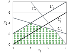
Figure 1: The plot represents a typical integer programming problem consisting of two variables $x_{1}$ and $x_{2}$ with three constraints ($C_{1}$, $C_{2}$, and $C_{3}$). The cost function $C_{f}$ is maximized to solve the problem while satisfying the constraints. The dotted region depicts the allowed solution space.

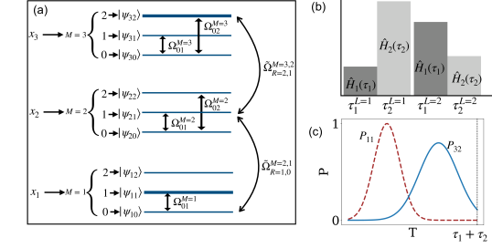
Figure 2: The figure summarizes the algorithm for solving IP problems using a multi-level system. (a) Depicts the implementation of variables along with the constraints of the IP problem using internal ($\Omega$) and external ($\tilde{\Omega}$) couplings for a multi-level Rydberg atom. $M=1,2,3$ represents three manifolds corresponding to the individual variables. The value that each variable can take is associated with the population of the relevant internal state belonging to a manifold as discussed in the text. (b) Schematically shows the coupling Hamiltonians $\hat{H_{1}}(\tau_{1})$ and $\hat{H_{2}}(\tau_{2})$ used to evolve an initial state, used for describing constraints as shown in Eqs. (5-6). The height of the shaded rectangle indicates the strength of the coupling while the width is the evolution time, both of which are varied in the optimization procedure. During the optimization, the coupling Hamiltonians are applied repeatedly and the iterations are indicated by $L$. (c) Shows the population transfer from one state to another during the first layer of the protocol in time $\tau_{1}+\tau_{2}$. $P_{11}$ and $P_{32}$ correspond to the population of the states $\psi_{11}$ and $\psi_{32}$ (shown as states with thick blue lines in panel a) respectively, and they represent the value of the variables $x_{1}=1$ and $x_{3}=2$.

II Theory and algorithmic implementation

In this section, we introduce the integer programming (IP) problem in II.1. A mapping of a general IP problem to the energy levels of an atom and the steps of the algorithm is provided in subsection II.2. The algorithm discussed in subsection II.3 is discussed using the specific physical settings of a Rydberg atom. The complexity of the different types of IP problems is discussed by identifying relevant benchmarking metrics in subsection II.4.

II.1 Integer programming

An integer programming (IP) problem is an optimization problem, such that the decision variables are constrained to take integer values Wolsey (2020). A typical IP problem is depicted in Fig. 1, the problem has two variables $x_{1},x_{2}$ and three constraints $C_{1},C_{2},C_{3}$. The highlighted area is called a feasible region as all the constraints are satisfied and the extremal of the cost function $C_{f}$ should always lie in the feasible region.

Consider $m$ optimizing variables $\mathbf{x}:=(x_{1},...,x_{m})$, coefficients $\mathbf{c}:=(c_{1},...,c_{m})$, $A$ be a $n\times m$ matrix, describing $n$ constraints and the condition on the constraints $\mathbf{b}:=(b_{1},...,b_{n})$. The integer programming problem to maximize the cost function $C_{f}(\mathbf{x})$ can be represented as

$$C_{f}(\mathbf{x})=c_{1}x_{1}\cdots x_{p}+\cdots+c_{m}x_{m}\cdots x_{p^{\prime}},$$ (1)

where $p,p^{\prime}\in\mathbb{Z}^{+}$ and $x_{i}\in\mathbb{Z}$, under the constraints given as

$$\begin{aligned} C_{1}:a_{11}x_{1}\cdots x_{q}+\cdots+a_{1m}x_{m}\cdots x_{q^{\prime}}\leq b_{1}\\ \vdots&\\ C_{n}:a_{nm}x_{1}\cdots x_{r}+\cdots+a_{nm}x_{m}\cdots x_{r^{\prime}}\leq b_{n}\end{aligned}$$ (2)

where $q,q^{\prime},r,r^{\prime}\in\mathbb{Z}^{+}$. If $p,p^{\prime},q,q^{\prime},r,r^{\prime}=1$, then the objective function and the constraints in the problem are linear and the problem is termed integer linear programming (ILP) otherwise it falls into the non-linear integer programming (NLIP) category. Any constraint with greater than equal to inequality can be converted to less than equal to inequality by multiplying $-1$ on both sides, hence the above description covers all the cases.

Typically, Branch and Bound is a widely used technique for solving IP problems classically Beale and Small (1965). It involves breaking down the problem into smaller subproblems, solving them individually, and using bounds to reduce the search space efficiently. Branch and Cut is an extension of the branch and bound method that incorporates cutting planes to tighten the bounds on the solution space Sen and Sherali (2006). The classical solvers used to solve a general MIP problem can be broadly categorized as B&B-based and simplex-based. Both approaches have their advantages and shortcomings based on the type of IP problem that is being solved. B&B-based solvers run into issues if the relative continuous relaxation gap increases for a problem, requiring a large number of iterations. In comparison, simplex-based solvers are mostly used to solve linear problems. Any non-linear problem is first converted into a linear one for the simplex algorithm application, the whole process becomes computationally expensive. There are many classical algorithms available to solve IP problems Bliek1ú et al. (2014), but due to the complexity of the problem, there is a potential to take advantage of the quantum systems. Currently, there are no quantum schemes that leverage the inherent structure of any quantum system to efficiently encode and solve IP problems, except for translating the problem to QUBO form. In our work, the IP problem is encoded on a single atom and solved for small instances, the details are in the next section.

II.2 An algorithm for solving integer programming

To demonstrate the fundamental principles of our approach, a sample problem containing three variables, $x_{i}\in\{0,1,2\}$ and two constraints is considered,

$$\begin{split}C_{f}(\mathbf{x})=3x_{1}+2x_{2}+x_{3}\\ C_{1}:2x_{1}+x_{2}\leq 3\\ C_{2}:x_{2}+x_{3}\leq 2\end{split}$$ (3)

A multi-level quantum system whose population can be controlled with an external field is used for describing the steps of the algorithm. The algorithm includes encoding the integer variables onto the multi-level setup of a quantum system and implementation of the constraints of the problem through couplings of the levels.

Step 1: Mapping of the variables onto the internal states - The variables in the IP problem $x_{i=1,2,3}$ are one-to-one mapped to different energy manifolds $M=1,2,3$ consisting of multiple states as shown in Fig. 2(a). Since the variable $x_{i}\in\{0,1,2\}$, this corresponds to each manifold $M=i$ consisting of three states $\ket{\psi_{i0}},\ket{\psi_{i1}}$ and $\ket{\psi_{i2}}$ with values assigned as $v_{0}=0,v_{1}=1$ and $v_{2}=2$ respectively. If one of the variables in another example were to take values in $\{0,1\}$, the corresponding manifold would contain two states encoding the values. The population of the states in each manifold is measured to decode the value of the corresponding variables. The state with the highest population in the manifold determines the integer value of that particular variable. For example, in $M=1$ there are three states whose population can be measured. The state with the highest population in $M=1$ will determine the value of the variable $x$, which is assigned as $\ket{\psi_{10}}\xrightarrow{}0,\ket{\psi_{11}}\xrightarrow{}1,\ket{\psi_{12}}\xrightarrow{}2$. Similarly, comparing the population of the states in other manifolds determines the value of the variables encoded in them. Fig. 2(c) shows the population of the states $\psi_{11}$ and $\psi_{32}$ at different times, which is measured to be dominant and finds the value of variables $x_{1}=1$ and $x_{2}=2$ respectively.

Step 2: Mapping of the constraints - Any implementation of the constraint in the problem is divided into three parts, restricting the values of the individual variables, constructing the relationship between the variables, and satisfying the inequalities. For example, constraint $C_{1}:2x_{1}+x_{2}\leq 3$ does not allow $x_{1}=2$, as it will violate the inequality directly and two variables $x_{1}$, $x_{2}$ together need to satisfy the constraint. To implement the constraint $C_{1}$ physically, the key idea is to couple the internal states of a manifold corresponding to the allowed values of that particular variable and externally couple the states in different manifolds in order to establish the relationship between the variables for a given constraint. Finally, all the couplings are optimized to satisfy the inequalities in the given constraint.

Specifically, the internal couplings are used within a manifold to restrict populating specific states that are excluded by the problem constraint. For example, in Eq. (3), the constraint $C_{1}$, $x_{1}=2$ is not allowed which translates to only coupling $\ket{\psi_{10}}$ and $\ket{\psi_{11}}$ states in the manifold $M=1$ which avoids populating the state $\ket{\psi_{12}}$. The coupling term $\Omega_{01}^{M=1}$ as shown in Fig. 2(a) is used for associating selective states where $\Omega_{ij}^{M}$ describes the coupling of the internal states of $M$. $\Omega_{ij}^{M}$ provides a control that can be optimized to reach a configuration corresponding to the inequality being satisfied. As for variable $x_{2}$, both $\Omega_{01}^{M=2}$ and $\Omega_{02}^{M=2}$ are non-zero as it can take any value in $\{0,1,2\}$. The external couplings are between different manifolds to implement the relationship between the variables, $x_{1}$ and $x_{2}$ in $C_{1}$. By tuning external couplings $\tilde{\Omega}_{M,i}^{R,j}$, the population of the states of $M=2$ and $R=1$ manifolds redistribute and in turn couples the variables $x_{1}$ and $x_{2}$. Similarly for another constraint $C_{2}:x_{2}+x_{3}\leq 2$, $\tilde{\Omega}_{M,i}^{R,j}$ will couple $M=2$ and $R=3$ for the mapping. The allowed couplings will depend on the states chosen in each manifold as shown schematically in Fig. 2(a).

The coupling Hamiltonian is given by,

$$\begin{split}\hat{H}=\sum_{M,k,R,l}(\tilde{\Omega}^{M,l}_{R,k}\ket{\psi_{Rk}}\bra{\psi_{Ml}}+h.c.)\\ +\sum_{M,i,j}(\Omega^{M}_{ij}\ket{\psi_{Mi}}\bra{\psi_{Mj}}+h.c.),\end{split}$$ (4)

where $\ket{\psi_{Mk}}$ is the state $k$ in manifold $M$. The external couplings of the states of one manifold $R$, $\ket{\psi_{Rk}}$ to the states in the other manifold $M$, $\ket{\psi_{Ml}}$ are described by the first term in $\hat{H}$. The constraints for individual variables are given by the internal coupling of the states $\ket{\psi_{Mi}}$ to $\ket{\psi_{Mj}}$ in manifold $M$, corresponding to the second term. For a given problem, the number of required internal and external couplings are predefined and hence many of the terms in $\hat{H}$ will vanish. The steps outlined for mapping the problem apply to any integer programming problem, both for linear and non-linear cases.

In general, multiple inequalities need to be satisfied, which requires a coupling Hamiltonian $\hat{H_{i}}$ for each constraint $C_{i}$. However, the inequalities must be fulfilled simultaneously to solve the problem. The coupling Hamiltonians for the constraints $C_{1}$ and $C_{2}$ of the example problem are given as,

$$\begin{split}\hat{H_{1}}=\tilde{\Omega}^{M=1,0}_{R=2,1}\ket{\psi_{10}}\bra{\psi_{21}}+\Omega^{M=1}_{01}\ket{\psi_{10}}\bra{\psi_{11}}\\ +\Omega^{M=2}_{01}\ket{\psi_{20}}\bra{\psi_{21}}+\Omega^{M_{2}}_{02}\ket{\psi_{20}}\bra{\psi_{22}}\\ +h.c.,\end{split}$$ (5)

$$\begin{split}\hat{H_{2}}=\tilde{\Omega}^{M=2,1}_{R=3,2}\ket{\psi_{21}}\bra{\psi_{32}}+\Omega^{M=2}_{01}\ket{\psi_{20}}\bra{\psi_{21}}\\ +\Omega^{M=2}_{02}\ket{\psi_{20}}\bra{\psi_{22}}+\Omega^{M=3}_{01}\ket{\psi_{30}}\bra{\psi_{31}}\\ +\Omega^{M=3}_{02}\ket{\psi_{30}}\bra{\psi_{32}}+h.c..\end{split}$$ (6)

For the example problem 3, an initial state is chosen with a population of $\ket{\psi_{10}}$ state be $1$. $\ket{\psi_{initial}}=(p_{10},p_{11},...,p_{32}):(1,0,...,0)$ where $p_{ij}$ describes the population of the state $\ket{\psi_{ij}}$. Then we apply $\hat{H_{1}}$ for time $\tau_{1}$ and $\hat{H_{2}}$ for time $\tau_{2}$ to evolve the initial state as $\hat{H_{2}}\hat{H_{1}}\ket{\psi_{initial}}$, which describes a layer $L$, shown in Fig. 2(b). While the choice of couplings determines the implementation of the inequalities, the layering helps in population mixing and multiple such layers with the same Hamiltonians are constructed. The choice of the states that need to be coupled, time $\tau$, and the strength of the couplings are to be optimized to fulfill all the constraints simultaneously while finding the maximal cost function which is described in the next step.

Step 3: Optimization of the objective function - The quantum optimal control requires the initialization of the parameters that are iteratively varied to find the minima of an objective function. In our case, the coupling strengths $\Omega,\tilde{\Omega}$ and the time $\tau$ corresponding to each Hamiltonian are parameters that are initially chosen to an arbitrary value, and the number of layers $L$ is predefined for each problem. Through an iterative process, optimal values of these parameters are found using an optimizer that can be gradient-based, non-gradient-based, or a combination of both. The results for these optimal parameters are shown in the section III, where different prototypical problems are solved. The sum of all the values for $\tau$ corresponds to the total time $T$ of the optimal protocol, where $T$ is not fixed. The variation in the couplings results in the selective population transfer of the states. The integer variables are decoded from the population of the manifolds, and then the cost function that needs to be optimized is calculated. We can determine the time interval for which all the inequalities are satisfied and form a set $S_{\tau}$ consisting of those time points, for example, the shaded region in Fig. 4(a). The goal is to minimize the objective function $O$, which can be calculated from the variables decoded from the population. The objective function contains two parts, satisfying all the constraints simultaneously and maximizing the cost function $C_{f}$ of the problem Kuroś et al. (2021); Krauss et al. (2023). The multi-objective function is defined as

$$O=(1-\frac{N_{\tau}}{N_{T}})+(1-\frac{\sum_{t\in S_{\tau}}C_{f}(t)}{\sum_{t=0}^{t=T}C_{f}(t)}),$$ (7)

where $T$ is the total time of the protocol, $N_{T}$ is the total number of discretized time points of $T$, $S_{\tau}$ is a set containing time points where all the inequalities/constraints are satisfied, $N_{\tau}$ is the cardinality of the set $S_{\tau}$, and $C_{f}(t)$ is the cost function that needs to be maximized in the integer programming problem. The first term of the objective function maximizes $N_{\tau}$ i.e. the total time for which all the constraints are simultaneously satisfied ensuring that the system remains for a longer duration in the feasible region of the IP problem. The second term maximizes the sum of the cost function at all times in the feasible region ($t\in S_{\tau}$), which increases the probability of finding the optimal solution during the measurement in an experiment and contributes to the robustness of the protocol. It is essential to normalize each term in $O$ to prevent bias toward one of the objectives which can result in skewed-inaccurate results. The multi-objective function is then minimized using a combination of a gradient (BFGS) Broyden (1970); Fletcher (1970); Goldfarb (1970); Shanno (1970) and non-gradient (Nelder-mead) Nelder and Mead (1965) based optimal control methods to find the optimal values of the couplings. There exist other quantum optimal control methods such as Bayesian optimization that can also be used Mukherjee et al. (2020a, b). In the end, the protocol provides those time intervals when the population measurement followed by decoding the value of the variables will result in the optimal solution.

Figure 3: The table in (a) shows the chosen sample integer programming problems that are encoded and solved using multi-levels of a single Rydberg atom. The problems with varied complexity (as explained in the section II.4) depend on the problem type and the number of variables. The corresponding benchmark metrics Kronqvist et al. (2019) are shown in (b-d) panels, where the black dot indicates the complexity of the problems as defined in panel (a).

II.3 Physical implementation in a Rydberg atom

The simulation of synthetic dimensions on a multi-level Rydberg atom Kanungo et al. (2022) provides a platform for encoding the IP problem. The precise occupation of these levels can be controlled by applying external fields Sundar et al. (2018); Ozawa and Price (2019); Kanungo et al. (2022). Each dimension or a collection of closely spaced energy eigenstates is referred to as a manifold. There are internal couplings between the states of each manifold and external couplings between the states of different manifolds. Selectively populating and creating a superposition of states of a multi-level system allows us to implement integer programming problems. In principle, any quantum system can be used for implementing our algorithm, and here are the steps of our protocol for a single Rydberg atom.

Initialization: A Rydberg atom with the principal quantum numbers $n=56,...,62$, and angular momentum $l=0,1$ is considered for simulation. Initial state preparation involves a population transfer from the atom’s ground state to one of the Rydberg states participating in the multi-level transitions. For the example problem given by Eq. (3), each manifold consists of 3 states corresponding to the constraint on each variable $x_{i}=0,1,2$. To allow maximum flexibility in terms of transitions, the three states representing $x_{0}=0$: $nS$, $x_{1}=1$: $nP$, and $x_{2}=2$: $(n+1)P$ are chosen. The next manifold, representing another variable contains the states $n^{\prime}S$, $n^{\prime}P$ and $(n^{\prime}+1)P$, where $n\neq n^{\prime}$ and $n\neq n^{\prime}+1$, holds for the states. The following assignment for the Rydberg states can be used for applying the algorithm to the example problem.

$$\begin{split}\ket{\psi_{10}}\xrightarrow{}\ket{nS},\ket{\psi_{11}}\xrightarrow{}\ket{nP},\ket{\psi_{12}}\xrightarrow{}\ket{(n+1)P}\\ \ket{\psi_{20}}\xrightarrow{}\ket{n^{\prime}S},\ket{\psi_{21}}\xrightarrow{}\ket{n^{\prime}P},\ket{\psi_{22}}\xrightarrow{}\ket{(n^{\prime}+1)P}\\ \ket{\psi_{30}}\xrightarrow{}\ket{n^{\prime\prime}S},\ket{\psi_{31}}\xrightarrow{}\ket{n^{\prime\prime}P},\ket{\psi_{32}}\xrightarrow{}\ket{(n^{\prime\prime}+1)P}\\ \end{split}$$ (8)

Probing: The Hamiltonian for the coupling of the states in a single Rydberg atom with detuning $\Delta=0$ is given by Eq. (4), thereby neglecting the counter-rotating terms in the couplings, transforming into a rotating frame and absorbing the constants in the couplings. The states are coupled through microwave lasers with Rabi frequencies $\Omega$ and $\tilde{\Omega}$. Selectively populating Rydberg atoms is analogous to having a multilevel extension of the electromagnetically induced transparency process Mohapatra et al. (2007). Other ways to control the state populations can involve the use of stimulated Raman adiabatic passage (STIRAP) Cubel et al. (2005). By employing optimal quantum control methods, similar to our algorithm, other approaches can be used to efficiently populate the states Kanungo et al. (2022).

Measurement: After populating the states for solving a given problem, the task is to make repeated measurements to efficiently decode the values of the variables. The measurement of the populations can either be done by selective field ionization ($\mu s$ time scales) Gallagher et al. (1977) or time-resolved measurements ($ns-\mu s$ time scales) Cetina et al. (2016). Particularly, for measuring the population of the states in the Rydberg atoms, selective field ionization can be performed with tens of $V/cm$ electric field strength and within a time scale of a few $\mu s$ Kanungo et al. (2022). The time it takes for the measurement can be brought down by increasing the electric field strength or by choosing a different principal quantum number $n$ for the Rydberg states. The population measurement time for our algorithm (discussed in the Results section III) is well within the reach of the current experimental capabilities.

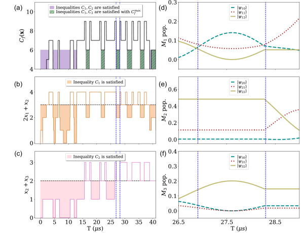
Figure 4: Integer linear programming problem: maximize $C_{f}(\mathbf{x})=3x_{1}+2x_{2}+x_{3}$ where constraints are $x_{i}\in\{0,1,2\}$, $C_{1}:2x_{1}+x_{2}\leq 3$ and $C_{2}:x_{2}+x_{3}\leq 2$. $C_{f}=6$ is the true solution to the problem calculated by considering all the possible values of the variables. (a) depicts the value of the cost function of the problem with the shaded region (purple and green with slanted lines) corresponding to the time when both inequalities are satisfied simultaneously. The shaded green-slanted-line region represents the time intervals for which the optimal value of the cost function is reached while satisfying the constraints. Panels (b-c) show the implementation of the two constraints of the problem, both constraints are implemented using different coupling Hamiltonians. The shaded regions in (b) and (c) correspond to the time intervals when the constraint inequalities are individually satisfied. The two vertical blue-dashed lines mark the time interval for which the population plots in (d-f) for different manifolds are shown. The state with the highest population assigns the value to the variables which are then used to calculate $C_{f},C_{1}$, and $C_{2}$.

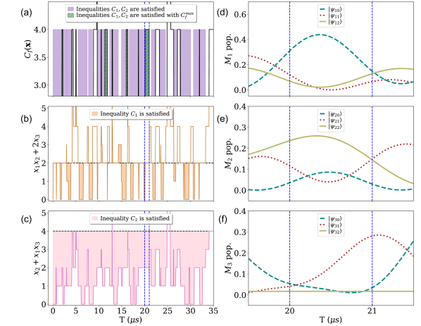
Figure 5: Non-linear integer programming problem: maximize $C_{f}(\mathbf{x})=2x_{2}x_{3}$ where constraints are $x_{i}\in\{0,1,2\}$, $C_{1}:x_{1}x_{2}+2x_{3}\leq 2$ and $C_{2}:x_{2}+x_{1}x_{3}\leq 4$. $C_{f}=4$ is the true solution to the problem calculated by considering all the possible values of the variables. In (a) the value of the non-linear cost function of the problem is shown with the shaded region (including the ones with slanted lines) corresponding to the time when both inequalities are satisfied simultaneously. (b) and (c) shows the implementation of the constraints of the problem and shaded regions in (b) and (c) correspond to the time intervals when the constraint inequalities are satisfied. The two vertical lines mark the time interval for which the population plots in (d-f) for different manifolds are shown.

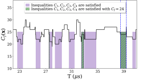
Figure 6: Integer linear programming problem: maximize $C_{f}(\mathbf{x})=x_{1}+2x_{2}+x_{3}+4x_{4}+3x_{5}+x_{6}+2x_{7}+5x_{8}$ where constraints are $x_{i}\in\{0,1,2\}$, $C_{1}:x_{1}+x_{2}+x_{3}\leq 1$, $C_{2}:2x_{4}+3x_{8}\geq 5$, $C_{3}:2x_{5}+2x_{6}+x_{7}\leq 3$, and $C_{4}:x_{3}+x_{7}\leq 1$. $C_{f}=25$ is the solution to the problem calculated using a brute force approach. (a) shows the cost function for $P_{3}$ in Fig. 3(a), with the shaded region corresponding to satisfying all the inequalities, and the green region (with slanted lines) showing the near-optimal solution.

II.4 Complexity of the problem

We now discuss the computational complexity and the difficulty of solving different instances of the problem. MIP problems transition from the P-complexity class (without integer constraints) to NP-hard (with integer constraints) due to the added complexity of exploring discrete solution spaces. The NP-hardness of the problems can be classified in a hierarchy as BIP $\subset$ ILP $\subset$ MILP $\subset$ MINLP, where B is binary, L stands for linear and NL stands for non-linear. Integer constraints often make the problem non-convex Wolsey and Nemhauser (1999), which results in standard convex optimization techniques that work efficiently for continuous problems no longer being applicable. The properties of the feasible region of a problem define convexity (or non-convexity). The constraints describe the boundaries of the feasible region for a problem and the objective function is then maximized or minimized in that region. If the constraints do not enclose any overlapping region then the problem becomes infeasible as all the constraints cannot be simultaneously satisfied. However, the concavity in the feasible region can encompass multiple local optima, saddle points, or discontinuities, making it harder for the standard solvers to navigate the optimization landscape. The complexity of the problems can also vary from one instance to another, one of the trivial metrics is the size of the NP-hard problem. In this section, three parameters Kronqvist et al. (2019) are discussed that can be used to encapsulate the difference in the difficulty of solving a general IP problem.

The relative continuous relaxation gap is one of the benchmark metrics that captures the difference between the optimal solution of the IP problem and the relaxed IP problem, defined as

$$B_{1}=\frac{|V_{int}-V_{cont}|}{max\{|V_{int}|,0.001\}}\crossproduct 100\%,$$ (9)

where $V_{int}$ is the optimal value of the integer problem and $V_{cont}$ is the optimal value of the corresponding continuous relaxed problem. Many classical algorithms solve the relaxed problem (non-linear or linear continuous programming) as the initial step for solving the given IP problem. It is known that the continuous programming problem can be solved in polynomial time. The problems considered in this work are benchmarked using the branch & bound algorithm. The problem with a larger gap $B_{1}$ (same number of variables) requires more nodes for convergence, highlighting the relevance even for problems with a small number of variables.

Non-linearity in the problem can make it intractable and a quadratic IP problem is undecidable and cannot have any algorithm to solve it Jeroslow (1973). While solving the non-linear problems the classical algorithms do not always converge even if the problem is decidable due to the presence of many local minima. The common IP solvers struggle to solve NLIP problems, and suffer from inaccurate solutions and large computing times as compared to the ILP counterparts Kronqvist et al. (2019). In the case of branch & bound, there is an explosion in the number of nodes for a modest size problem, limiting the size of the NILP that can be solved classically. The degree of non-linearity is defined as Kronqvist et al. (2019),

$$B_{2}=\frac{n}{n_{tot}}\crossproduct 100\%,$$ (10)

where $n$ is the number of variables involved in a non-linear term and $n_{tot}$ is the total number of variables. In general, other metrics such as the degree of non-convexity of the optimization landscape can be defined for measuring the complexity. Non-convexity can be captured indirectly by combining $B_{1}$ and $B_{2}$, as non-linearity directly contributes to a complex landscape and a large relative relaxation gap can be a consequence of a non-convex hull.

Lastly, discrete density provides a measure of the number of discrete variables present in the problem. When integer values are introduced in a linear programming problem, the complexity class changes from P to NP-hard. Hence for any two integer programming problems, the one with more discrete variables will be harder to solve and the metric discrete density becomes relevant, defined as, Kronqvist et al. (2019),

$$B_{3}=\frac{n_{int}+n_{bin}}{n_{tot}}\crossproduct 100\%,$$ (11)

where $n_{int}$ and $n_{bin}$ are the number of integer and binary discrete variables respectively and $n_{tot}$ is the total number of variables. This parameter is useful for categorizing the complexity of different MIP problems. The problems shown in Fig. 3(a) are categorized based on the complexity via the metrics discussed in this section, also represented by the black dots in Fig. 3(b),(c), and (d). The chosen prototypical problems are solved, and the results are discussed in the next section.

III Results

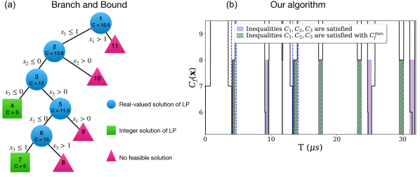
Figure 7: Integer linear programming problem: max $C_{f}(\mathbf{x})=8x_{1}+7x_{2}+6x_{3}$ where constraints are $x_{i}\in\{0,1,2\}$, $C_{1}:3x_{1}+x_{2}+3x_{3}\leq 5$, $C_{2}:x_{1}+2x_{2}+x_{3}\leq 3$ and $C_{3}:4x_{2}+x_{3}\leq 2$. $C_{f}=8$ is the true solution to the problem calculated by considering all the possible values of the variables. (a) shows the classical branch and bound method for solving the problem and (b) shows the cost function for the problem and the optimal solution using our algorithm. The regions between the dotted (vertical) lines correspond to the solution of the problem for extended intervals of time.

To demonstrate the mapping and the working principle of our algorithm, we consider a simple ILP problem as the first example whose optimal solution and the corresponding populations of the states are shown in Fig. 4. The chosen problem corresponds to the example IP Eq. (3) containing three integer variables and two linear constraints ($P_{1}$ from Table 3(a)). The coupling Hamiltonians (Eqs. (5-6)) corresponding to the two constraints $C_{1},C_{2}$ are applied consecutively to evolve an initial state in time, with couplings being time-dependent. Panel (a) shows the cost function $C_{f}$ changing in time (solid black line) where the true solution to the problem is given by $C_{f}=6$. The multi-objective function is minimized to find the maximum of $C_{f}$ while satisfying both the constraints $C_{1},C_{2}$ shown as the shaded regions in panel (a). Time intervals where both constraints are satisfied correspond to filled regions when the value of the cost function reaches maxima is shown as green-shaded regions with slanted lines in panel (a). Similarly, the individual constraints (solid lines) and their corresponding inequality fulfilled time intervals (shaded) are depicted, $C_{1}\leq 3$ in panel (b) and $C_{2}\leq 2$ in panel (c). Panels (d-f) show the populations of the states in manifolds $M={1,2,3}$ for the region between the two vertical dashed (panels a-c) blue lines. The population of the states $\ket{\psi_{10}}$, $\ket{\psi_{22}}$, and $\ket{\psi_{32}}$ in panels (d),(e) and (f) respectively are the highest during the time interval enclosed between the vertical blue lines, assigning the values $x_{1}=0$, $x_{2}=2$, and $x_{3}=2$ respectively. In this way the cost function $C_{f}$ and the constraints $C_{1},C_{2}$ are then calculated by decoding the variables by the measurement of the populations. Next, we consider a more complex case as an example problem.

Fig. 5 shows the flexibility of our algorithm by solving a problem with a non-linear cost function and constraints. The sample integer programming problem is intentionally chosen to test our scheme on a harder problem, refer to Eq. (10) ($P_{2}$ in Fig. 3(a)). In Fig. 5, panel (a) shows the exact optimal solution of the problem given at times marked by the shaded green region (with slanted lines) while panels (b) and (c) correspond to the individual constraints. The protocol scheme follows the same steps as described for the previous problem. Although the optimal solution is reached at $T\sim 2\mu s$ as shown by the earliest green (slanted lines) region in panel (a), however, we chose to show the longest green (with lines) interval for better understanding. The population of the states during the interval bounded by the two dashed-blue lines are shown in panels (d-f). The population of the states gives the value of the variables $x_{1}=0$ ($\ket{\psi_{10}}$ in panel d), $x_{2}=2$ ($\ket{\psi_{22}}$ in panel e) and $x_{3}=2$ ($\ket{\psi_{32}}$ in panel f) that are used to calculate the cost function that is $C_{f}=4$. For constraint $C_{2}$, any state of any manifold can be populated while for $C_{1}$, $x_{3}=2$ is forbidden, translating to state $\ket{\psi_{32}}$ not being coupled to any other state.

Until now the examples contained only three variables, the complexity due to the increase in size of the problem is shown by solving the next problem. The problem we consider has eight variables and four constraints whose cost function is shown in Fig. 6, where the green regions (with slanted lines) correspond to the near-optimal solution $C_{f}=24$, and the true solution is $C_{f}=25$. The chosen problem, $P_{3}$ in Fig. 3(a), is more complicated as compared to the previous examples since the complexity of the IP problem increases exponentially with the number of discrete variables $B_{3}$ (depicted in Fig. 3(d)). This complexity results in the frequency and the width of the green-slanted-line regions for solving $P_{3}$ (Fig. 6) being less as compared to a simpler problem of three variables $P_{1}$ (Fig. 4a). However, the near-optimal solution is reached in $40\mu s$, and the system remains in this configuration for more than $1\mu s$. We also reach the true solution $C_{f}=25$ with a different set of parameters that lasts for $0.1\mu s$ (not shown here) for which the states stay in the optimal configuration. The shaded regions correspond to the times when all the inequalities are satisfied and the cost function during those time intervals has many sub-optimal solutions. For instance, during $T\sim 32-35$, the cost function $C_{f}=22$ is somewhat close to the optimal solution $C_{f}=25$.

To benchmark the performance of our algorithm, an implementation of branch & bound (B&B) is considered which is shown in Fig. 7. The classical B&B is used to solve the problem $P_{4}$ from Fig. 3(a), which required $11$ nodes (iterations) to converge as opposed to our one-shot algorithm. Panel (a) in Fig. 7 shows the explicit nodes involved in the B&B algorithm. Circular blue nodes are intermediate steps, where the problem branches into sub-problems with additional constraints on the variables. B&B relies upon solving the relaxed problem and bounding the solution space by constraining the problem. The IP problem is relaxed to have continuous variables, and the solution of the continuous problem provides an upper bound for the solution of IP. A lower bound is found by assigning integer values to the optimal continuous variables ($v_{1},...,v_{n}$). The continuous variable (e.g., $x_{i}$) with the largest fractional part is chosen to branch and solve the problem at two nodes, such that Node 1: $x_{i}\leq\lfloor v_{i}\rfloor$ and Node 2: $x_{i}>\lfloor v_{i}\rfloor$. In panel (a), the upper bound of the cost function at each node is given by the value $C$ which kept decreasing after the subsequent branching, and the lower bound did not change for the problem $P_{4}$. The complexity of $P_{4}$ is captured by the high $B_{1}=93\%>50\%$ value Kronqvist et al. (2019), corresponding to the large difference in the solution of the relaxed continuous problem and the discrete IP. For comparison, problem $P_{1}$ has $B_{1}=8.3\%$ and it converges after $3$ nodes in B&B to the optimal solution. In general, if the value of $B_{1}$ is higher for a problem, it takes more branches for the upper bound to converge to the integer solution. The branching can be terminated in three ways, (1) the optimal solution contains all the integer variables as shown by green squares in panel (a), (2) the relaxed problem becomes infeasible under the constraints corresponding to the pink triangles, and (3) the stopping criteria of either the maximum number of nodes or the maximum time are reached, which is required when the problem has a high relative continuous relaxation gap. Many state-of-the-art solvers use one of the implementations of the B&B algorithm, hence they also suffer when one of the parameters Eqs. (9,10,11) becomes larger for different instances of the problem. The algorithm for the given problem $P_{4}$ terminates after $11$ nodes and the optimal solution, $C=8$ with $(x_{1},x_{2},x_{3})=(1,0,0)$ for $P_{4}$, is the highest value of the cost function in the green squares. Panel (b) shows the result of our algorithm, in which the solution is reached as early as $5\mu s$ during the first layer of the Hamiltonians, which is clearly better than the B&B in terms of the number of iterations required for convergence. An alternative hybrid approach for problems with a larger number of variables would be to use B&B and apply our algorithm to provide tighter bounds as compared to solving the relaxed problem.

IV Conclusions and Outlook

Implementation of most of the algorithms on a quantum system requires a large number of qubits and they rely upon the quantum entanglement of a many-body system to gain an advantage over classical methods. Alternatively, an advantage can potentially be achieved by exploiting the superposition principle as is done in this work. Generally, combinatorial optimization problems can be formulated mathematically either as a quadratic binary unconstrained optimization (QUBO) or an IP problem. The architecture of the current quantum devices makes QUBO formulation a more popular choice for executing algorithms, however, IP is widely used to formulate industrial optimization problems due to it being more efficient in terms of the number of variables. To solve an IP problem on a quantum device, QUBO is used as a stepping stone, which is an indirect approach, thus increasing the number of qubits required. We provide a few examples of methods to solve IP on a quantum system, Khosravi et al. (2023) considers a problem with three binary variables with a probability $85-90\%$ for finding the solution, while in Zhao et al. (2022), a problem with two discrete variables are encoded with a solution not better than the classical counterpart of the algorithm and in Bernal et al. (2020b), a linear graph of two nodes for solving minimum dominating set problem, required 5 qubits to get a solution with probability $90-95\%$. Our approach for the first time, introduces a non-QUBO-based algorithm by directly mapping the IP problem to a quantum system and solving it by exploiting the superposition principle. It opens up a new pathway of encoding and algorithmic processing within a single atom. The algorithm we provide can handle both linear and non-linear IP problems and requires a single atom to implement it.

We chose a few prototype problems with varying complexities characterized by the benchmarking metrics namely, relative continuous relaxation gap, degree of non-linearity, discrete density, and size of the problem. The problems are then encoded to a multi-level Rydberg atom with each manifold of states representing integer variables. The manifolds are probed and selectively populated by optimizing the coupling strength between the different levels for implementing the problem’s constraints. The population of the states is then measured to decode the optimal values of the integer variables to find the solution of the problem which is reached in microseconds $\mu s$ with high accuracy. A comparison is made with the classical B&B algorithm, and our algorithm performed better for a problem with a large relative continuous relaxation gap. The direct algorithm solved the problem in a one-shot approach while the B&B algorithm needed $11$ nodes to converge. The classical algorithms suffer more in terms of resources and accuracy for solving non-linear problems as compared to the linear problems Kronqvist et al. (2019).

There are a few ways in which a larger problem can be solved under our framework, which is the outlook for this work. One atom is used in our algorithm to solve a problem with $8$ variables, if we use hundreds of atoms, in principle that can encode a problem with thousands of variables. The constraints can be implemented by mediating the interaction between different atoms. All the computations can then be performed in parallel thereby decreasing the time for solving the large problem. Another possible approach would be to divide the larger IP problem into sub-problems using the Benders decomposition Rahmaniani et al. (2017). But instead of solving the relaxed continuous sub-problems using classical B&B to bound the solution space, we can provide better bounds by solving the integer (without relaxation) sub-problems on the individual atoms in parallel. This can provide better approximate solutions and enhance the bounds provided by the branch and bound method. For comparison, the state-of-the-art classical solver (BARON), solves a non-convex mixed non-linear IP problem with $2500$ variable in $300s$ Kronqvist et al. (2019). In this way, we have the perspective of solving problems where the current classical algorithms struggle.