A Lagrangian Perspective on Growth of Midlatitude Storms
Abstract
Extratropical storms dominate midlatitude climate and weather and are known to grow baroclinicaly and decay barotropicaly. Understanding how their growth responds to climatic changes is crucial for accurately quantifying climate and weather in the extratropics. To date, quantitative climatic measures of storms’ growth have been mostly based on Eulerian measures, taking into account the mean state of the atmosphere and how those affect eddy growth, but they do not consider the Lagrangian growth of the storms themselves. Here, using ERA-5 reanalysis data and tracking all extratropical storms (cyclones and anticyclones) from over 80 years of data, we examine the actual growth of the storms and compare it to the Eulerian characteristics of the mean state as the storms develop. We find that, in the limit of weak baroclinicity, measures such as the Eulerian Eady Growth Rate provide a good measure of the storms’ actual strength. However, for high baroclinicity levels, this linear relationship breaks. We show that while the actual growth rate of single storms is linearly correlated with the Eulerian measures, the high baroclinicity reduction in storm strength is due to a decrease in the storms’ growth time with baroclinicity. Based on the Lagrangian analysis, we suggest a nonlinear correction to the traditional Eady Growth Rate. Expanding the analysis to include the mean flow’s barotropic properties highlights their marginal effect on storms’ growth rate but the crucial impact on growth time. Our results emphasize the potential of Lagrangianly studying many storms to advance understanding of the midlatitude climate.
AGU Advaces
Department of Earth and Planetary Sciences, Weizmann Institute of Science, Rehovot, Israel
Or Hadasor.hadas@weizmann.ac.il
To uncover the relation between the mean flow and storm growth, we analyze Lagrangianly all midlatitude storms from 83 years of ERA5 data.
While the Lagrangian growth rate is found to increase linearly with the Eady Growth Rate, the storm growth time exhibits an opposite trend.
We propose a non-linear general relation between the local mean flow characteristics of the atmosphere and the strength of storms.
Plain Language Summary
The midlatitude climate is shaped by storms. Their growth is primarily driven by baroclinic instability, a process converting vertical wind shear into storms’ energy. Understanding how climatic changes impact this growth is essential for advancing midlatitude climate and weather understanding. In this study, we systematically evaluated the growth of storms using ERA-5 reanalysis data and tracks of all storms over 83 years. The Lagrangian growth of storms is compared to the Eady Growth Rate, a traditional measure of the midlatitude large-scale vertical wind shear. While a linear correlation between the Eady Growth Rate and storm energy is observed under mild jet strength, this relationship breaks down under extreme jet conditions. While the actual growth of storms is found to correlate to the Eady Growth Rate linearly, this deviation is attributed to a decrease in the storms’ growth time with the Eady Growth Rate. As a result, a nonlinear correction to the traditional Eady Growth Rate is proposed for intense jet conditions. Expanding the analysis to include the horizontal wind shear emphasizes its minimal impact on storm growth rate, but underscores its crucial influence on growth time. These results highlight the importance of systematic study of large quantities of storms.
1 Introduction
The midlatitude momentum, heat, and moisture fluxes display significant spatial variability, primarily concentrated in regions referred to as the “storm track” (Chang \BOthers., \APACyear2002; Hoskins \BBA Hodges, \APACyear2005, \APACyear2019). Three primary storm tracks have been identified: the Northern Hemisphere (NH) Atlantic and Pacific storm tracks and the Southern Hemisphere (SH) storm track. From a Lagrangian perspective, this spatial variability arises from substantial differences in cyclonic and anticyclonic activity among various parts of the world, serving as the main driver for the weather variability experienced by communities throughout the midlatitudes. Moreover, the midlatitude weather displays a significant temporal variability, which is primarily seasonal. The seasonal variability is characterized by a general pattern of migration equatorward and intensification from summer to winter. The interplay between spatial and temporal variations adds another layer of complexity. For instance, the Atlantic storm track significantly strengthens from summer to winter, the SH storm track maintains relatively constant intensity, and the Pacific storm track strengthens from summer to autumn, but weakens during winter (Nakamura, \APACyear1992; Okajima \BOthers., \APACyear2022).
The spatial and temporal variations described above result from numerous physical processes, including the seasonal alterations in solar insolation, surface and atmospheric albedo, emissivity, oceanic forcing, and interaction with orography. Due to their importance, these processes have been studied extensively, and their impact on the storm tracks is often deduced using a three-step process (e.g., Shaw \BOthers., \APACyear2016): first, the atmospheric flow is decomposed (using a spatial or temporal filter) into the mean flow, representing large-scale and slowly varying phenomena, such as jet streams, and eddy fields, dominated by cyclonic and anticyclonic activity. Second, the effect of the alterations in atmospheric forcing on the mean state of the atmosphere is assessed, which is manageable through modeling, statistics, and theoretical analysis due to the simplification achieved by averaging the atmosphere. Third, the storm tracks’ response is inferred based on the eddy state response to the changes in the mean state. However, because eddy fields are complex and nonlinear, there are no exact analytical solutions for their response, and numerical solutions heavily depend on the settings. Nevertheless, theoretical frameworks connecting the mean and eddy flow have emerged, including baroclinic instability models (e.g., Charney, \APACyear1947; Eady, \APACyear1949; Phillips, \APACyear1954), potential vorticity tendency decomposition (e.g., Hoskins \BOthers., \APACyear1985; Davis \BBA Emanuel, \APACyear1991; Tamarin \BBA Kaspi, \APACyear2017), and energetics analyses (e.g., Lorenz, \APACyear1955; Peixóto \BBA Oort, \APACyear1974; Okajima \BOthers., \APACyear2022).
These approaches are usually applied from an Eulerian perspective, measuring the resulting global or regional changes in eddy activity following a change in the mean state of the atmosphere and interpreting it through theoretical frameworks. For example, Nakamura \BBA Sampe (\APACyear2002) suggested that extremely strong jet streams cause a disconnect between the upper-level eddies and the surface, which suppresses baroclinic conversion. Harnik \BBA Chang (\APACyear2004) showed using idealized models that the jet’s strengthening and narrowing during winter has an opposite effect on the Eddy Kinetic Energy (EKE). Caballero \BBA Hanley (\APACyear2012) illustrated that EKE is reduced in warmer climates, which is one of the main drivers of decreased poleward moisture transport. Additionally, Schemm \BBA Rivière (\APACyear2019) revealed that the intense midwinter jet over the Pacific, which results from the extreme meridional temperature, diminishes the efficiency of baroclinic conversion by altering the interaction between eddy heat flux and baroclinicity.
While the Eulerian approach plays an important role in our understanding of the midlatitude climate, it has significant limitations. For instance, analyses that average physical properties combining the mean and eddy flow (e.g., the energy conversion terms described in Sec. 2.1) make it impossible to isolate their relative contributions to the response, significantly limiting causal inference. In addition, Eulerian averages mix the contribution from various atmospheric phenomena (cyclones, anticyclones, atmospheric rivers, dry intrusions, etc.), making it challenging to infer the actual changes in weather patterns underlying the Eulerian response. The Lagrangian perspective, allowing better causal inference and being more closely related to weather patterns, has proven useful in uncovering crucial aspects of the mechanism behind complex atmospheric phenomena (e.g., Tamarin-Brodsky \BBA Kaspi, \APACyear2017; Tamarin-Brodsky \BBA Hadas, \APACyear2019; Schemm \BOthers., \APACyear2021; Hadas \BBA Kaspi, \APACyear2021; Tsopouridis \BOthers., \APACyear2021; Kang \BBA Son, \APACyear2021; Okajima \BOthers., \APACyear2021, \APACyear2022, \APACyear2024; Hadas \BOthers., \APACyear2023).
Previous studies of the Lagrangian response to the mean flow were conducted either using case studies (e.g., Orlanski \BBA Katzfey, \APACyear1991; Rivière \BBA Joly, \APACyear2006), which show real-world dynamics, but are limited in their ability to conduct a systematic investigation, idealized simulations (e.g., Orlanski \BBA Chang, \APACyear1993; Rivière \BOthers., \APACyear2013; Hadas \BBA Kaspi, \APACyear2021), which allow systematic investigation, but their relevance to real-life dynamics is limited, or focused on a specific geographical location (e.g., Schemm \BOthers., \APACyear2020; Tsopouridis \BOthers., \APACyear2021; Okajima \BOthers., \APACyear2023), and therefore strongly depends on the specific configuration of the area. Therefore, the primary objective of this study is to understand the general response of individual cyclones and anticyclone (also hereby referred to jointly as ’systems’) growth to atmospheric forcing using a systematic statistical analysis of real atmospheric data. More specifically, we examine how Eulerian properties of the mean flow, commonly used as proxies for baroclinic growth, impact the actual Lagrangian growth of cyclones and anticyclones. Knowledge about individual systems is acquired using a storm tracking algorithm (Sec. 2.3, Hodges, \APACyear1995), which obtains the position and intensity of cyclones and anticyclones throughout their lifetime. The tracking algorithm is applied to 83 years of ERA-5 data (Sec. 2.2), providing a state-of-the-art evaluation of atmospheric conditions. The analysis considers cyclones and anticyclones from all storm tracks and seasons, allowing the exploration of the full range of atmospheric mean states observed in Earth’s current climate. Moreover, incorporating systems worldwide and across all seasons provided us with over 100,000 cyclones and 50,000 anticyclones, enabling robust statistical analyses.
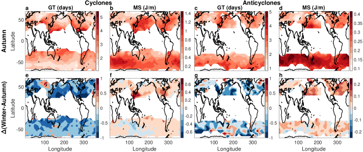
To gain insights into the response of individual cyclones and anticyclones to the atmosphere’s mean state, the spatial and temporal variability in their Growth Time (GT, defined as the time between detection and maximum intensity of the system), and Maximum Strength (MS, calculated using Eq. 5 based on the pressure anomaly found by the tracking algorithm) is diagnosed (Fig. 1). Both properties exhibit spatial variability unique to each property and different between cyclones and anticyclones. For example, the autumn climatology of MS shows that the cyclones that live the longest are generated at low latitudes (around 30∘, Fig. 1a), while the anticyclones that live the longest are generated at high latitudes (around 50∘, Fig. 1c). In contrast, these patterns are flipped when considering the MS, meaning that the strongest cyclones are generated at high latitudes and the strongest anticyclones are generated at low latitudes (Fig. 1b and 1d, respectively). Both properties also undergo a distinct seasonal cycle. When comparing winter and autumn, GT decreases from autumn to winter (Fig. 1e,g), while the MS increases (Fig. 1f,h), particularly in the Northern Hemisphere. This emphasizes that MS and GT exhibit fundamentally different responses to changes in the mean flow.
In this study, we explore how the spatial and temporal variability in cyclones’ and anticyclones’ properties arises from the response of individual cyclones and anticyclones to the atmospheric mean state. Utilizing a Lagrangian approach, we establish connections between the properties of cyclones and anticyclones and the baroclinic and barotropic characteristics of the mean flow (Sec. 2 provides a detailed discussion of the methods). We begin by studying the response of the systems’ properties to the baroclinic characteristics of the mean flow through the commonly used Eady Growth Rate (EGR, Sec. 3.1). Then, we extend the analysis to include the barotropic characteristics of the flow, quantifying the relative importance of each property of the mean flow and exploring the differences in the properties’ response between cyclones and anticyclones (Sec. 3.2).
2 Methods
2.1 Energetic perspective
To estimate the impact of the mean state of the atmosphere on the growth of cyclones and anticyclones, an energetics perspective is adopted. Our focus is on the interaction between the mean and eddy fields, specifically the conversion of mean available potential energy to eddy available potential energy (baroclinic conversion) and the conversion of EKE to mean kinetic energy (barotropic conversion). By neglecting vertical advection, these terms can be expressed as follows (Peixóto \BBA Oort, \APACyear1992; Kosaka \BBA Nakamura, \APACyear2006; Schemm \BBA Rivière, \APACyear2019; Okajima \BOthers., \APACyear2022):
| (1) | ||||
| (2) |
where and are the conversion between eddy and mean potential and kinetic energy, respectively, and are the zonal and meridional components of the wind, respectively, is pressure, is the gravitational constant, is the Coriolis parameter, is the density of air, is temperature, is the Brunt-Väisälä frequency, and is the radius of Earth.
The conversion budget terms can be decomposed into a product between an eddy and mean parts. Then, the impact of the mean flow on the eddy flow can be isolated by considering only the mean part of the conversion terms and studying how it affects cyclones and anticyclones. These mean components are measured in rate units (day-1) and are proportional to the vertical and horizontal shear of the mean flow and, therefore, will be referred to as shear rates. From an idealized perspective, the shear rates can be interpreted as the barotropic and baroclinic energy conversion rate for a given anomaly energy (as the eddy part is proportional to the eddy terms to the second power, similar to the eddy energy).
When evaluating the baroclinic component of the shear rate, constant stratification and wind shear are assumed to eliminate the variability in the vertical dimension. Furthermore, the mean component of the wind is assumed to vanish at the surface because the surface wind is generally small and predicted poorly by the ERA-5 reanalysis (Belmonte Rivas \BBA Stoffelen, \APACyear2019). The resulting estimate for the baroclinic part is as follows:
| (3) |
where , R is the specific gas constant of dry air, is the potential temperature, the subscript refers to the pressure level of the field, and the bar is defined as a low-pass of 14 days. Note that the magnitude of this vector closely resembles the EGR and will henceforth be referred to as EGR. Barotropic conversion is the largest in the upper atmosphere (Peixóto \BBA Oort, \APACyear1992). Therefore, the mean flow at 300 hPa is used to assess the barotropic part of the shear rate:
| (4) |
where and are known as stretching deformation and shearing deformation, respectively (Mak \BBA Cai, \APACyear1989).
To establish a connection between the pressure anomaly (obtained through the tracking) and the surface kinetic energy associated with the cyclones and anticyclones (used as a proxy to the overall energy), a Gaussian pressure profile is assumed:
where is the pressure anomaly at the center of the system, is the distance from the center of the system, and is the length scale of decay. Then, the surface EKE associated with a given cyclone or anticyclone at a given time (assuming geostrophic balance) is:
| (5) |
where is the magnitude of the wind vector anomaly squared. The MS of storms is defined as the maximum measured for a given system.
2.2 Reanalysis data
Data from the European Center for Medium-Range Weather Forecasts ERA-5 reanalysis (Hersbach \BOthers., \APACyear2020) between 1940 and 2022 is used to assess the current climate. The ERA-5 estimates the atmospheric variables at a horizontal resolution of 31 km and 137 vertical levels. Three-hourly Sea Level Pressure (SLP) is used to identify the cyclones’ and anticyclones’ tracks. Three hourly temperature, geopotential, and horizontal wind data are used to estimate the different properties related to the energetics of cyclones and anticyclones. The data is down-sampled to 1.51.5∘.
2.3 Storm tracking and composites
A feature point tracking algorithm (Hodges, \APACyear1995; Tamarin \BBA Kaspi, \APACyear2016) applied on SLP data is used to identify and characterize extratropical cyclones and anticyclones. The data is smoothed to a T63 resolution to reduce noise. The background, defined as zonal wavenumbers 0-4, is removed to isolate the synoptic scale dynamics. Only SLP anomalies deeper than 8 hPa are tracked to account only for significant events. After identification, systems are tracked, and if they appear for more than 48 hours and propagate more than 500 km westward, their location and intensity are recorded. In addition, systems that peaked in intensity over topography higher than 1 km are also filtered out. Overall, about 100,000 cyclones and 50,000 anticyclones are included in the analysis.
To construct composites, a box with margins at a distance of 1500 km in the zonal direction and 670 km in the meridional direction from the center of the SLP anomaly is used. The meridional direction of SH systems is flipped to match the NH systems. The composites are averaged between the time the systems are identified and the maximum intensity. Compositing the barotropic and baroclinic properties of the mean flow around the storms through their growth phase allows to establish a connection between the mean flow and cyclones’ and anticyclones’ properties.
3 Results
3.1 The Lagrangian response to baroclinicity
The study begins by examining the influence of the baroclinic characteristics of the mean flow (baroclinicity), considered a primary driver of eddy flow growth, on the growth of individual cyclones and anticyclones. The tracking data is employed to construct composites of the EGR (as defined in Sec. 2.1), which are used to estimate the baroclinicity experienced by the systems. Then, the EGR composites are clustered in two iterations using a K-means algorithm (Pedregosa \BOthers., \APACyear2011). In the first iteration, normalization is applied to each cluster based on its mean and average, resulting in the clustering of the systems’ position relative to the jet (Fig. S1). For this iteration, three centroids are used, leading to clusters of cyclones and anticyclones observed equatorward (28% of cyclones, 67% of anticyclones), around the center (16% of cyclones, 15% of anticyclones), and poleward of jet core (55% of cyclones and 18% of anticyclones, Fig. S1a, S1b, and S1c, respectively).
Subsequently, the un-normalized EGR composites are clustered. This additional clustering layer mainly sorts the cyclones according to their composite average EGR. Only clusters containing more than 100 systems are retained to ensure adequate sample sizes. The benefit of this clustering method lies in its ability to isolate the effect of the magnitude and distribution of the EGR on cyclones’ and anticyclones’ properties, while effectively removing the influence of eddy-eddy interactions and other properties of the environment (such as surface properties). Following clustering, the centroid’s composite average EGR is calculated and regressed against the average properties of systems in the cluster.
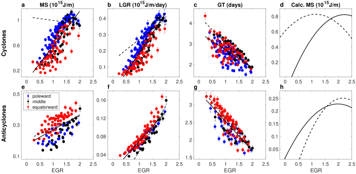
The cyclones’ MS (determined by Eq. 5, using the tracked pressure anomaly, Fig. 2a) exhibits a positive correlation of 0.75 with EGR (Pearson correlation). This finding aligns with our expectation that regions of enhanced baroclinicity, such as the storm tracks, would be associated with increased activity of cyclones and anticyclones. However, the positive correlation breaks at high EGR (around 1.5 day-1), and the correlation for only the top 20% baroclinicity clusters is -0.07. This saturation might play a significant role in the dynamics of regions characterized by extreme baroclinicity, such as the Eastern Pacific during midwinter (Nakamura, \APACyear1992). This saturation can explain, for example, why the cyclonic contribution to EKE saturates during midwinter (Okajima \BOthers., \APACyear2023) even though the track density peaks during midwinter (Okajima \BOthers., \APACyear2021). Another larger deviation from linearity is because cyclones on the poleward side of the jet are stronger (comparing blue, red, and black clusters in Fig. 2a).
The anticyclones’ MS is also positively correlated with EGR (0.54, Fig. 2e). The main departure from linearity for anticyclones is the substantial difference in MS at various parts of the baroclinic jet (Fig. 2e red versus blue and black). When examined individually for each region, the correlation ranges from 0.7 to 0.9, with anticyclones on the equatorward side of the jet being stronger.
To further study the anomalies in the MS-EGR relation, the MS is decomposed into GT and Lagrangian Growth Rate (LGR), defined as the actual average rate of intensification during the growth stage, as measured by the tracking algorithm. For cyclones, the LGR is better correlated with EGR (0.88, Fig. 2b) than the MS, especially for high EGR (0.40 for the top 20% of EGR values). The linear relation between EGR and LGR shows that, in Earth’s climate, the growth rate calculated by linear baroclinic instability models (e.g., Charney, \APACyear1947; Eady, \APACyear1949; Phillips, \APACyear1954) predicts well the actual Lagrangian growth of cyclones.
However, the GT of cyclones is negatively correlated with EGR (0.66, Fig. 2c). The reduction in GT with baroclinicity aligns with previous results from meteorological studies of the West Pacific (Schemm \BOthers., \APACyear2020) and the observation that GT reduces during winter (Fig. 1e). This trend was also observed in idealized simulations, which showed it resulted from the mean state’s effect on the baroclinic wave’s vertical structure (Hadas \BBA Kaspi, \APACyear2021). A comparison of GT and LGR between low and high baroclinicity values reveals that percentage-wise, LGR is increasing more rapidly (approximately a 400% increase between low and high baroclinicity values) than GT (about a 50% decrease). Cyclones on the poleward side of the jet have higher LGR and lower GT (Fig. 2b,c blue versus red), which explains the small overall difference in the MS on different sides of the jet (relative to anticyclones).
Similar to cyclones, the anticyclones’ LGR is better correlated with EGR (0.90, Fig. 2f) than the MS (0.54, Fig. 2e), and the GT decreases with EGR (correlation of -0.81, Fig. 2g). Anticyclones on the equatorward side of the jet have both a longer GT and a higher LGR (Fig. 2g, red versus blue), which explains why anticyclones on the poleward side of the jet are significantly stronger (Fig. 2e, blue versus red).
A linear model for the relationship of GT and LGR with EGR is fitted (Fig. 2b,c,f,g solid, the coefficients for cyclones and anticyclones are given in Tab. S1 and Tab. S2, respectively) to extrapolate how the increase in LGR and decrease in GT affects the MS at high baroclinicity regimes. The constant coefficient for LGR is very small, which fits our expectation that no baroclinicity will result in no growth. The main difference in the coefficients between cyclones and anticyclones is that the linear coefficient for the LGR is about four times larger for cyclones. In contrast, the fitted coefficients for the GT are remarkably similar.
Using the fitted coefficients, the MS is approximated as the multiplication of the two curves, which results in a parabola (Fig. 2d and 2h for cyclones and anticyclones, respectively). The resulting estimate for MS is given by:
| (6) | ||||
| (7) |
where the constant term of the LGR is neglected because it is small. The units of the linear coefficient is and of the second order coefficient is . From a physical point of view, the first term can be interpreted as the linear increase in MS due to the increase in LGR, while the second term can be interpreted as the nonlinear decrease in MS due to the decrease in GT. For low and medium values of EGR (0.5 day-1), the linear term contributes about eight times more than the nonlinear term, while for high EGR (2 day-1), it contributes only about two times more. This demonstrates why the linear approximation works well for most values of baroclinicity relevant to Earth’s climate, but breaks down for high baroclinicity values.
The optimal EGR for cyclones’ growth (i.e., the maximum of the solid parabola in Fig. 2d) is around 2 day-1. This value is slightly shifted from the observed value in the data. Fitting only the clusters in the top 20% of EGR (Fig. 2b,c dashed) results in a slower increase in LGR and a faster decrease in GT, shifting the maximum of the parabola around 1.3 day-1 (Fig. 2d dashed). This adjustment seems to fit the cluster data better. For anticyclones, the fitted LGR and GT curves (Fig. 2f and 2g solid, respectively), predict that the optimal EGR for the growth of anticyclones is around 2 day-1(Fig. 2h solid). In contrast to cyclones, fitting only clusters in the top 20% of baroclinicity does not result in a significant change in the fitted curves (Fig. 2f,g dashed). Therefore, the parabola resulting from the curve multiplication predicts a similar optimal EGR for growth (Fig. 2h dashed).
These findings indicate that the Lagrangian growth of cyclones and anticyclones fundamentally aligns with the predictions of linear baroclinic instability models, with the LGR increasing linearly with baroclinicity. However, the Lagrangian perspective unveils crucial details regarding the intricacy of the response. First, it reveals that cyclones’ MS, expected to correlate well with Eulerian EKE, linearly increases with EGR only for low and medium baroclinicity values. For high values of baroclinicity, there is a nonlinear decrease in MS for cyclones, resulting from the reduction in GT. Second, it demonstrates a significant difference in the growth of different phases of the baroclinic wave; specifically, cyclones exhibit much faster growth. Third, The Lagrangian perspective suggests that the barotropic shear of the mean flow substantially affects the Lagrangian properties. This topic is further explored in the next section.
3.2 The full Lagrangian response to the atmospheric mean state
The variability in LGR and GT for clusters with different spatial layouts of baroclinicity (Fig. 2b,c,f,g) suggest that the horizontal gradients of the mean flow, referred to as barotropic shear, significantly influence the growth of cyclones and anticyclones. This observation is supported by the results of previous studies (e.g., Lorenz, \APACyear1955; James, \APACyear1987; Rivière \BOthers., \APACyear2013). Therefore, in this section, the importance of the barotropic shear rates (, and ) is assessed and compared to the effect of baroclinic shear rates (, and ), as defined in Eq. 3 and 4. The response of LGR and GT to each shear rate component is quantified by sorting cyclones and anticyclones based on the composite average shear rates they experienced during their growth stage and studying the resulting differences in the average LGR and GT. Additionally, a 4-dimensional linear model is fitted to assess quantitatively the relative importance of each shear term (see Sec. S1).
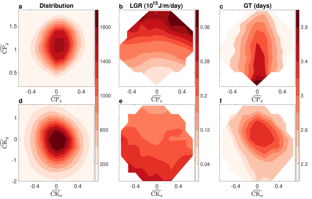
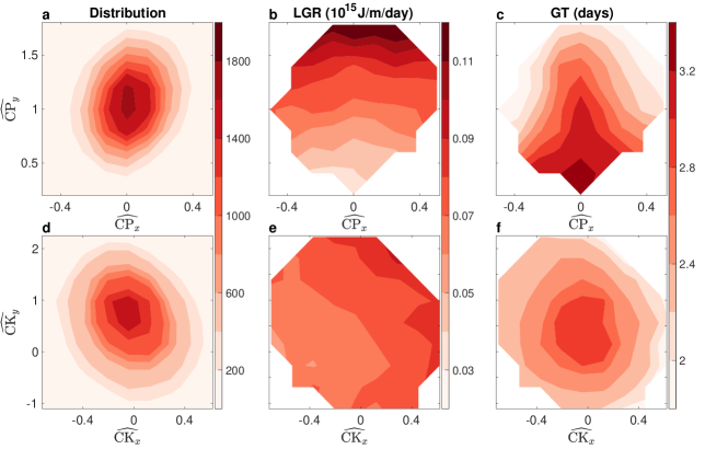
First, the distribution of cyclones and anticyclones in the shear rates space (, , , ) is analyzed. The shear rates of systems have a low correlation between them (in absolute value, lower than 0.08 for cyclones and lower than 0.25 for anticyclones, Tab. S3 and Tab. S4, respectively). Therefore, the coefficients can be treated, approximately, as independent variables. For cyclones, the distribution is centered around (0, 1.1, -0.1, 0.1) (Fig. 3a,d). For anticyclones, the distribution is centered around (0, 1.1, -0.1, 0.6) (Fig. 4a,d), and therefore the main difference between cyclones and anticyclones is that anticyclones tend to be strongly in positive . The variability is dominated by the meridional shear of zonal wind, where positive values of are associated with the equatorward side of the jet and vise versa. Therefore, the common positive values found for anticyclones fit the clustering analysis results (Sec. 3.1).
Comparing the contribution of the barotropic and baroclinic shear rates to cyclones’ LGR (Fig. 3b versus Fig. 3e), shows the baroclinic contribution is about twice. The effect of the baroclinic terms on cyclones’ LGR (Fig. 3b) shows that LGR is positively correlated with and the absolute value of . The increase in LGR with baroclinicity, seen in Fig. 2b is mostly due to . A linear model shows that for a given shear rate value, has an effect higher by 45% than . Given that the relevant range of values for is about three times larger in Earth’s climate, the is found to have a four times larger impact (comparing the variation in color between the ordinate and abscissa in Fig. 3b). Cyclones’ LGR is negatively correlated with both barotropic shear rates (Fig. 3e). Linear Regression analysis shows that has a 10% higher contribution than per unit of change. However, because the range is larger, it has an overall contribution that is around four times larger. Connecting back to Fig. 2b, the negative correlation between and LGR determines that cyclones on the poleward side of the jet have higher LGR, as is negative on the poleward side of the jet. Therefore, the difference in LGR between both sides of the jet is due to the opposing effect of barotropic shear.
For anticyclones, the baroclinic contribution to LGR is about four to five times larger (Fig. 4b versus Fig. 4e). The linear analysis shows that per unit of barotropic shear rate, is 65% more influential, and considering the larger range of values for , it makes it around five times more influential. Linear regression analysis shows that anticyclones’ LGR is positively correlated with the barotropic rate components, where has about three times a higher contribution to anticyclones’ LGR than per unit of change, but because range is larger, it has an overall contribution that is about the same. The positive correlation between the LGR and explains the fact that anticyclones on the equatorward side of the jet have a higher LGR.
The GT of cyclones reduces with both the baroclinic and barotropic shear rates (Fig. 3c and Fig. 3f, respectively). For the range of values relevant to Earth, the baroclinic shear rates explain about 20% more of the variability. The regression coefficients show that has a per-unit shear rate four times larger effect than , but because the range of relevant values of is about four times larger, they have an overall similar effect. Similarly, the regression coefficient is about three times larger, but because the range of relevant values is much larger for , the overall effect of both components is roughly similar. The general response of anticyclones’ GT to the shear rates (Fig. 4c versus Fig. 4f) is very similar: the baroclinic shear rates are more influential by about 90%, and the overall response due to the zonal and meridional components is similar.
Building upon the results of Sec. 3.1, the analysis above uncovers more crucial details of the effect of the mean flow on the growth of single cyclones and anticyclones: first, it shows that while the baroclinic properties of the flow dominate the LGR of cyclones and anticyclones, the GT is almost as influenced by the barotropic characteristics of the flow. These results are physically interpreted as the fastest breaking of the baroclinic structure of the system with stronger baroclinic and barotropic shear (Hadas \BBA Kaspi, \APACyear2021). Second, while the relatively weak mean meridional flow has a small effect on the LGR, it has a large effect on the GT, which might play a significant role in the effect of stationary waves on storm tracks (e.g., Kaspi \BBA Schneider, \APACyear2013). Third, comparing cyclones and anticyclones, the barotropic shear plays an opposing role on the LGR, which explains why cyclones on the poleward side of the jet are stronger while anticyclones on the equatorward side are stronger. Moreover, the barotropic properties of the mean flow play a more significant role in cyclones than in anticyclones.
4 Summary
When investigating the midlatitude climate’s response to changes in atmospheric forcing, whether natural or anthropogenic, a key challenge lies in understanding how eddies respond to the mean state of the atmosphere. While many studies have explored this interaction from an Eulerian perspective, there has yet to be a systematic exploration of how the mean state of the atmosphere impacts the growth of storms from a Lagrangian perspective. To fill this gap, our study delves into how the mean state of the atmosphere influences the growth of cyclones and anticyclones from a statistical point of view. Considering a massive database of 100,000 cyclones and 50,000 anticyclones from over 80 years of reanalysis data, we have enough statistics to quantify storms’ growth directly and compare them to the Eulerian theory.
Eulerian analysis of the Lagrangian properties shows that the Growth Time (GT) and Maximum Strength (MS) of cyclones and anticyclones exhibit fundamentally different temporal and spatial variations. For example, while MS increases in summer relative to autumn, GT decreases (Fig. 1). Studying the connection between MS and the vertical shear of the mean flow, using K-mean clustering of Eady Growth Rate (EGR ) composites, shows that MS mostly increases with baroclinicity. However, this trend flips for cyclones at extreme values of EGR (Fig. 2a), which play a significant role in the midlatitude weather response to extreme baroclinicity, such as over the North Pacific during midwinter.
The nonlinear response of MS to high EGR is further investigated by breaking down MS into the contributions from the Lagrangian Growth Rate (LGR) and GT. The LGR increases linearly with EGR (Fig. 2b,f), affirming that the growth rate predicted by linear baroclinic instability models aligns well with the observed Lagrangian growth. However, the LGR of anticyclones exhibited a slower increase than cyclones, showing that the different phases of the baroclinic wave grow at different rates. Furthermore, the GT is found to decrease with EGR (Fig. 2c,g). This implies that the linear increase in MS for most values of EGR is due to the rapid increase in LGR, while the decrease for extreme EGR, observed for cyclones, results from the nonlinearity introduced by the reduction in GT. The magnitudes of the linear and nonlinear terms are estimated through regression analysis of EGR on LGR and GT, and we propose a nonlinear correction to the classical connection between EGR and baroclinic activity based on the insights obtained from the Lagrangian perspective (Eq. 6,7).
The K-means clustering analysis also highlights the substantial influence of the horizontal shears of the mean flow on the growth of cyclones and anticyclones. To consider the effect of the barotropic characteristics of the mean flow and compare it to the baroclinic characteristics, cyclones and anticyclones are sorted according to mean shear rates around them (, , , ). , representing the baroclinic shear due to mean zonal flow, emerged as the primary contributor to LGR (Fig. 3b and Fig. 4b). The barotropic characteristic of the jet exerted a lesser impact on LGR, demonstrating opposing effects on cyclones and anticyclones (Fig. 3e versus Fig. 4e). The GT of cyclones and anticyclones proves to be strongly influenced by both the barotropic and baroclinic characteristics of the mean flow (Fig. 3c,f and Fig. 4c,f). These findings underscore the necessity of considering both barotropic and baroclinic properties when predicting the response of cyclones and anticyclones to the mean flow characteristics.
5 Open Research
5.1 Data Availability Statement
No new data sets were generated during the current study. ERA-5 is available through the Climate Data Store (cds.climate.copernicus.eu).
Acknowledgements.
This research has been supported by the Azrieli fellowship and The Israeli Science Foundation (Grant 996/20).References
- Belmonte Rivas \BBA Stoffelen (\APACyear2019) \APACinsertmetastarBelmonte2019{APACrefauthors}Belmonte Rivas, M.\BCBT \BBA Stoffelen, A. \APACrefYearMonthDay2019. \BBOQ\APACrefatitleCharacterizing ERA-Interim and ERA5 surface wind biases using ASCAT Characterizing ERA-Interim and ERA5 surface wind biases using ASCAT.\BBCQ \APACjournalVolNumPagesOcean Science153831–852. \PrintBackRefs\CurrentBib
- Caballero \BBA Hanley (\APACyear2012) \APACinsertmetastarCaballero2012{APACrefauthors}Caballero, R.\BCBT \BBA Hanley, J. \APACrefYearMonthDay2012\APACmonth11. \BBOQ\APACrefatitleMidlatitude Eddies, Storm-Track Diffusivity, and Poleward Moisture Transport in Warm Climates Midlatitude eddies, storm-track diffusivity, and poleward moisture transport in warm climates.\BBCQ \APACjournalVolNumPagesJ. Atmos. Sci.69113237-3250. \PrintBackRefs\CurrentBib
- Chang \BOthers. (\APACyear2002) \APACinsertmetastarChang2002{APACrefauthors}Chang, E\BPBIK\BPBIM., Lee, S.\BCBL \BBA Swanson, K\BPBIL. \APACrefYearMonthDay2002\APACmonth08. \BBOQ\APACrefatitleStorm Track Dynamics. Storm track dynamics.\BBCQ \APACjournalVolNumPagesJ. Climate152163-2183. \PrintBackRefs\CurrentBib
- Charney (\APACyear1947) \APACinsertmetastarcharney1947{APACrefauthors}Charney, J\BPBIG. \APACrefYearMonthDay1947. \BBOQ\APACrefatitleThe dynamics of long waves in a baroclinic westerly current The dynamics of long waves in a baroclinic westerly current.\BBCQ \APACjournalVolNumPagesJ. of Meteo.45136–162. \PrintBackRefs\CurrentBib
- Davis \BBA Emanuel (\APACyear1991) \APACinsertmetastarDavis1991{APACrefauthors}Davis, C\BPBIA.\BCBT \BBA Emanuel, K\BPBIA. \APACrefYearMonthDay1991. \BBOQ\APACrefatitlePotential Vorticity Diagnostics of Cyclogenesis Potential vorticity diagnostics of cyclogenesis.\BBCQ \APACjournalVolNumPagesMon. Weath. Rev.1191929. \PrintBackRefs\CurrentBib
- Eady (\APACyear1949) \APACinsertmetastarEady1949{APACrefauthors}Eady, E\BPBIT. \APACrefYearMonthDay1949\APACmonth08. \BBOQ\APACrefatitleLong Waves and Cyclone Waves Long waves and cyclone waves.\BBCQ \APACjournalVolNumPagesTellus133. \PrintBackRefs\CurrentBib
- Hadas \BOthers. (\APACyear2023) \APACinsertmetastarHadas2023{APACrefauthors}Hadas, O., Datseris, G., Blanco, J., Bony, S., Caballero, R., Stevens, B.\BCBL \BBA Kaspi, Y. \APACrefYearMonthDay2023. \BBOQ\APACrefatitleThe role of baroclinic activity in controlling Earth’s albedo in the present and future climates The role of baroclinic activity in controlling Earth’s albedo in the present and future climates.\BBCQ \APACjournalVolNumPagesProc. Natl. Acad. Sci. U.S.A.1205e2208778120. \PrintBackRefs\CurrentBib
- Hadas \BBA Kaspi (\APACyear2021) \APACinsertmetastarHadas2021{APACrefauthors}Hadas, O.\BCBT \BBA Kaspi, Y. \APACrefYearMonthDay2021. \BBOQ\APACrefatitleSuppression of Baroclinic Eddies by Strong Jets Suppression of baroclinic eddies by strong jets.\BBCQ \APACjournalVolNumPagesJ. Atmos. Sci.. \PrintBackRefs\CurrentBib
- Harnik \BBA Chang (\APACyear2004) \APACinsertmetastarHarnik2004{APACrefauthors}Harnik, N.\BCBT \BBA Chang, E\BPBIK\BPBIM. \APACrefYearMonthDay2004\APACmonth01. \BBOQ\APACrefatitleThe Effects of Variations in Jet Width on the Growth of Baroclinic Waves: Implications for Midwinter Pacific Storm Track Variability. The effects of variations in jet width on the growth of baroclinic waves: Implications for midwinter Pacific storm track variability.\BBCQ \APACjournalVolNumPagesJ. Atmos. Sci.6123-40. \PrintBackRefs\CurrentBib
- Hersbach \BOthers. (\APACyear2020) \APACinsertmetastarHersbach2020{APACrefauthors}Hersbach, H., Bell, B., Berrisford, P., Hirahara, S., Horányi, A., Muñoz-Sabater, J.\BDBLothers \APACrefYearMonthDay2020. \BBOQ\APACrefatitleThe ERA5 global reanalysis The ERA5 global reanalysis.\BBCQ \APACjournalVolNumPagesQ. J. R. Meteorol. Soc.1467301999–2049. \PrintBackRefs\CurrentBib
- Hodges (\APACyear1995) \APACinsertmetastarhodges_1995{APACrefauthors}Hodges, K. \APACrefYearMonthDay1995. \BBOQ\APACrefatitleFeature tracking on the unit sphere Feature tracking on the unit sphere.\BBCQ \APACjournalVolNumPagesMon. Weath. Rev.123123458–3465. \PrintBackRefs\CurrentBib
- Hoskins \BBA Hodges (\APACyear2019) \APACinsertmetastarHoskins2019{APACrefauthors}Hoskins, B.\BCBT \BBA Hodges, K. \APACrefYearMonthDay2019. \BBOQ\APACrefatitleThe annual cycle of Northern Hemisphere storm tracks. Part I: Seasons The annual cycle of Northern hemisphere storm tracks. Part I: Seasons.\BBCQ \APACjournalVolNumPagesJ. Climate3261743–1760. \PrintBackRefs\CurrentBib
- Hoskins \BBA Hodges (\APACyear2005) \APACinsertmetastarhoskins2005{APACrefauthors}Hoskins, B\BPBIJ.\BCBT \BBA Hodges, K\BPBII. \APACrefYearMonthDay2005. \BBOQ\APACrefatitleA new perspective on Southern Hemisphere storm tracks A new perspective on Southern Hemisphere storm tracks.\BBCQ \APACjournalVolNumPagesJ. Climate18204108–4129. \PrintBackRefs\CurrentBib
- Hoskins \BOthers. (\APACyear1985) \APACinsertmetastarHoskins1985{APACrefauthors}Hoskins, B\BPBIJ., McIntyre, M\BPBIE.\BCBL \BBA Robertson, A\BPBIW. \APACrefYearMonthDay1985. \BBOQ\APACrefatitleOn the use and significance of isentropic potential vorticity maps On the use and significance of isentropic potential vorticity maps.\BBCQ \APACjournalVolNumPagesQ. J. R. Meteorol. Soc.111470877–946. \PrintBackRefs\CurrentBib
- James (\APACyear1987) \APACinsertmetastarJames1987{APACrefauthors}James, I\BPBIN. \APACrefYearMonthDay1987. \BBOQ\APACrefatitleSuppression of baroclinic instability in horizontally sheared flows Suppression of baroclinic instability in horizontally sheared flows.\BBCQ \APACjournalVolNumPagesJ. Atmos. Sci.443710-3720. \PrintBackRefs\CurrentBib
- Kang \BBA Son (\APACyear2021) \APACinsertmetastarKang2021b{APACrefauthors}Kang, J\BPBIM.\BCBT \BBA Son, S\BHBIW. \APACrefYearMonthDay2021. \BBOQ\APACrefatitleDevelopment processes of the explosive cyclones over the Northwest Pacific: Potential Vorticity tendency inversion Development processes of the explosive cyclones over the Northwest Pacific: Potential vorticity tendency inversion.\BBCQ \APACjournalVolNumPagesJ. Atmos. Sci.7861913–1930. \PrintBackRefs\CurrentBib
- Kaspi \BBA Schneider (\APACyear2013) \APACinsertmetastarKaspi2013b{APACrefauthors}Kaspi, Y.\BCBT \BBA Schneider, T. \APACrefYearMonthDay2013. \BBOQ\APACrefatitleThe role of stationary eddies in shaping midlatitude storm tracks The role of stationary eddies in shaping midlatitude storm tracks.\BBCQ \APACjournalVolNumPagesJ. Atmos. Sci.702596-2613. \PrintBackRefs\CurrentBib
- Kosaka \BBA Nakamura (\APACyear2006) \APACinsertmetastarKosaka2006{APACrefauthors}Kosaka, Y.\BCBT \BBA Nakamura, H. \APACrefYearMonthDay2006. \BBOQ\APACrefatitleStructure and dynamics of the summertime Pacific–Japan teleconnection pattern Structure and dynamics of the summertime Pacific–Japan teleconnection pattern.\BBCQ \APACjournalVolNumPagesQ. J. R. Meteorol. Soc.1326192009–2030. \PrintBackRefs\CurrentBib
- Lorenz (\APACyear1955) \APACinsertmetastarLorenz1955{APACrefauthors}Lorenz, E\BPBIN. \APACrefYearMonthDay1955. \BBOQ\APACrefatitleAvailable potential energy and the maintenance of the general circulation Available potential energy and the maintenance of the general circulation.\BBCQ \APACjournalVolNumPagesTellus7157-167. \PrintBackRefs\CurrentBib
- Mak \BBA Cai (\APACyear1989) \APACinsertmetastarMak1989{APACrefauthors}Mak, M.\BCBT \BBA Cai, M. \APACrefYearMonthDay1989. \BBOQ\APACrefatitleLocal barotropic instability Local barotropic instability.\BBCQ \APACjournalVolNumPagesJ. Atmos. Sci.46213289–3311. \PrintBackRefs\CurrentBib
- Nakamura (\APACyear1992) \APACinsertmetastarNakamura1992{APACrefauthors}Nakamura, H. \APACrefYearMonthDay1992\APACmonth09. \BBOQ\APACrefatitleMidwinter Suppression of Baroclinic Wave Activity in the Pacific. Midwinter suppression of baroclinic wave activity in the Pacific.\BBCQ \APACjournalVolNumPagesJ. Atmos. Sci.491629-1642. \PrintBackRefs\CurrentBib
- Nakamura \BBA Sampe (\APACyear2002) \APACinsertmetastarNakamura2002{APACrefauthors}Nakamura, H.\BCBT \BBA Sampe, T. \APACrefYearMonthDay2002\APACmonth08. \BBOQ\APACrefatitleTrapping of synoptic-scale disturbances into the North-Pacific subtropical jet core in midwinter Trapping of synoptic-scale disturbances into the North-Pacific subtropical jet core in midwinter.\BBCQ \APACjournalVolNumPagesGeophys. Res. Lett.298-1. \PrintBackRefs\CurrentBib
- Okajima \BOthers. (\APACyear2021) \APACinsertmetastarOkajima2021{APACrefauthors}Okajima, S., Nakamura, H.\BCBL \BBA Kaspi, Y. \APACrefYearMonthDay2021. \BBOQ\APACrefatitleCyclonic and anticyclonic contributions to atmospheric energetics Cyclonic and anticyclonic contributions to atmospheric energetics.\BBCQ \APACjournalVolNumPagesScientific reports1111–10. \PrintBackRefs\CurrentBib
- Okajima \BOthers. (\APACyear2022) \APACinsertmetastarOkajima2022{APACrefauthors}Okajima, S., Nakamura, H.\BCBL \BBA Kaspi, Y. \APACrefYearMonthDay2022. \BBOQ\APACrefatitleEnergetics of Transient Eddies Related to the Midwinter Minimum of the North Pacific Storm-Track Activity Energetics of transient eddies related to the midwinter minimum of the North Pacific storm-track activity.\BBCQ \APACjournalVolNumPagesJ. Climate3541137–1156. \PrintBackRefs\CurrentBib
- Okajima \BOthers. (\APACyear2023) \APACinsertmetastarOkajima2023{APACrefauthors}Okajima, S., Nakamura, H.\BCBL \BBA Kaspi, Y. \APACrefYearMonthDay2023. \BBOQ\APACrefatitleDistinct roles of cyclones and anticyclones in setting the midwinter minimum of the North Pacific eddy activity: a Lagrangian perspective Distinct roles of cyclones and anticyclones in setting the midwinter minimum of the North Pacific eddy activity: a Lagrangian perspective.\BBCQ \APACjournalVolNumPagesJ. Climate36144793–4814. \PrintBackRefs\CurrentBib
- Okajima \BOthers. (\APACyear2024) \APACinsertmetastarOkajima2024{APACrefauthors}Okajima, S., Nakamura, H.\BCBL \BBA Kaspi, Y. \APACrefYearMonthDay2024. \BBOQ\APACrefatitleAnticyclonic suppression of the North Pacific transient eddy activity in midwinter Anticyclonic suppression of the North Pacific transient eddy activity in midwinter.\BBCQ \APACjournalVolNumPagesGeophys. Res. Lett.512e2023GL106932. \PrintBackRefs\CurrentBib
- Orlanski \BBA Chang (\APACyear1993) \APACinsertmetastarOrlanski1993{APACrefauthors}Orlanski, I.\BCBT \BBA Chang, E\BPBIK\BPBIM. \APACrefYearMonthDay1993\APACmonth01. \BBOQ\APACrefatitleAgeostrophic Geopotential Fluxes in Downstream and Upstream Development of Baroclinic Waves. Ageostrophic geopotential fluxes in downstream and upstream development of baroclinic waves.\BBCQ \APACjournalVolNumPagesJ. Atmos. Sci.50212-225. \PrintBackRefs\CurrentBib
- Orlanski \BBA Katzfey (\APACyear1991) \APACinsertmetastarOrlanski1991{APACrefauthors}Orlanski, I.\BCBT \BBA Katzfey, J. \APACrefYearMonthDay1991\APACmonth09. \BBOQ\APACrefatitleThe Life Cycle of a Cyclone Wave in the Southern Hemisphere. Part I: Eddy Energy Budget. The life cycle of a cyclone wave in the southern hemisphere. Part I: Eddy energy budget.\BBCQ \APACjournalVolNumPagesJ. Atmos. Sci.481972-1998. \PrintBackRefs\CurrentBib
- Pedregosa \BOthers. (\APACyear2011) \APACinsertmetastarScikit-learn{APACrefauthors}Pedregosa, F., Varoquaux, G., Gramfort, A., Michel, V., Thirion, B., Grisel, O.\BDBLDuchesnay, E. \APACrefYearMonthDay2011. \BBOQ\APACrefatitleScikit-learn: Machine Learning in Python Scikit-learn: Machine learning in Python.\BBCQ \APACjournalVolNumPagesJournal of Machine Learning Research122825–2830. \PrintBackRefs\CurrentBib
- Peixóto \BBA Oort (\APACyear1974) \APACinsertmetastarPeixoto1974{APACrefauthors}Peixóto, J\BPBIP.\BCBT \BBA Oort, A\BPBIH. \APACrefYearMonthDay1974. \BBOQ\APACrefatitleThe annual distribution of atmospheric energy on a planetary scale The annual distribution of atmospheric energy on a planetary scale.\BBCQ \APACjournalVolNumPagesJ. Geophys. Res.79152149–2159. \PrintBackRefs\CurrentBib
- Peixóto \BBA Oort (\APACyear1992) \APACinsertmetastarPeixoto1992{APACrefauthors}Peixóto, J\BPBIP.\BCBT \BBA Oort, A\BPBIH. \APACrefYear1992. \APACrefbtitlePhysics of Climate Physics of climate. \APACaddressPublisherAmerican Institute of Physics. \PrintBackRefs\CurrentBib
- Phillips (\APACyear1954) \APACinsertmetastarPhillips1954{APACrefauthors}Phillips, N\BPBIA. \APACrefYearMonthDay1954. \BBOQ\APACrefatitleEnergy transformations and meridional circulations associated with simple baroclinic waves in a two level quasi-geostrophic model Energy transformations and meridional circulations associated with simple baroclinic waves in a two level quasi-geostrophic model.\BBCQ \APACjournalVolNumPagesTelus6273-286. \PrintBackRefs\CurrentBib
- Rivière \BOthers. (\APACyear2013) \APACinsertmetastarRiviere2013{APACrefauthors}Rivière, G., Gilet, J\BHBIB.\BCBL \BBA Oruba, L. \APACrefYearMonthDay2013. \BBOQ\APACrefatitleUnderstanding the regeneration stage undergone by surface cyclones crossing a midlatitude jet in a two-layer model Understanding the regeneration stage undergone by surface cyclones crossing a midlatitude jet in a two-layer model.\BBCQ \APACjournalVolNumPagesJ. Atmos. Sci.7092832–2853. \PrintBackRefs\CurrentBib
- Rivière \BBA Joly (\APACyear2006) \APACinsertmetastarRiviere2006{APACrefauthors}Rivière, G.\BCBT \BBA Joly, A. \APACrefYearMonthDay2006. \BBOQ\APACrefatitleRole of the low-frequency deformation field on the explosive growth of extratropical cyclones at the jet exit. Part I: Barotropic critical region Role of the low-frequency deformation field on the explosive growth of extratropical cyclones at the jet exit. Part I: Barotropic critical region.\BBCQ \APACjournalVolNumPagesJ. Atmos. Sci.6381965–1981. \PrintBackRefs\CurrentBib
- Schemm \BBA Rivière (\APACyear2019) \APACinsertmetastarschemm2019efficiency{APACrefauthors}Schemm, S.\BCBT \BBA Rivière, G. \APACrefYearMonthDay2019. \BBOQ\APACrefatitleOn the Efficiency of Baroclinic Eddy Growth and How It Reduces the North Pacific Storm-Track Intensity in Midwinter On the efficiency of baroclinic eddy growth and how it reduces the North Pacific storm-track intensity in midwinter.\BBCQ \APACjournalVolNumPagesJ. Climate32238373–8398. \PrintBackRefs\CurrentBib
- Schemm \BOthers. (\APACyear2020) \APACinsertmetastarSchemm2020{APACrefauthors}Schemm, S., Wernli, H.\BCBL \BBA Binder, H. \APACrefYearMonthDay2020. \BBOQ\APACrefatitleThe North Pacific Storm-Track Suppression Explained From a Cyclone Life-Cycle Perspective The North Pacific storm-track suppression explained from a cyclone life-cycle perspective.\BBCQ \APACjournalVolNumPagesWeather and Climate Dynamics Discussions1–19. \PrintBackRefs\CurrentBib
- Schemm \BOthers. (\APACyear2021) \APACinsertmetastarSchemm2021{APACrefauthors}Schemm, S., Wernli, H.\BCBL \BBA Binder, H. \APACrefYearMonthDay2021. \BBOQ\APACrefatitleThe storm-track suppression over the Western North Pacific from a cyclone life-cycle perspective The storm-track suppression over the Western North Pacific from a cyclone life-cycle perspective.\BBCQ \APACjournalVolNumPagesWeather and Climate Dynamics2155–69. \PrintBackRefs\CurrentBib
- Shaw \BOthers. (\APACyear2016) \APACinsertmetastarShaw2016{APACrefauthors}Shaw, T\BPBIA., Baldwin, M., Barnes, E\BPBIA., Caballero, R., Garfinkel, C\BPBII., Hwang, Y\BPBIT.\BDBLVoigt, A. \APACrefYearMonthDay2016\APACmonth09. \BBOQ\APACrefatitleStorm track processes and the opposing influences of climate change Storm track processes and the opposing influences of climate change.\BBCQ \APACjournalVolNumPagesNature Geo.9656-664. \PrintBackRefs\CurrentBib
- Tamarin \BBA Kaspi (\APACyear2016) \APACinsertmetastarTamarin2016a{APACrefauthors}Tamarin, T.\BCBT \BBA Kaspi, Y. \APACrefYearMonthDay2016\APACmonth04. \BBOQ\APACrefatitleThe Poleward Motion of Extratropical Cyclones from a Potential Vorticity Tendency Analysis The poleward motion of extratropical cyclones from a potential vorticity tendency analysis.\BBCQ \APACjournalVolNumPagesJ. Atmos. Sci.731687-1707. \PrintBackRefs\CurrentBib
- Tamarin \BBA Kaspi (\APACyear2017) \APACinsertmetastarTamarin2017mechanisms{APACrefauthors}Tamarin, T.\BCBT \BBA Kaspi, Y. \APACrefYearMonthDay2017. \BBOQ\APACrefatitleMechanisms controlling the downstream poleward deflection of midlatitude storm tracks Mechanisms controlling the downstream poleward deflection of midlatitude storm tracks.\BBCQ \APACjournalVolNumPagesJ. Atmos. Sci.742553–572. \PrintBackRefs\CurrentBib
- Tamarin-Brodsky \BBA Kaspi (\APACyear2017) \APACinsertmetastarTamarin-Brodsky2017{APACrefauthors}Tamarin-Brodsky, T.\BCBT \BBA Kaspi, Y. \APACrefYearMonthDay2017\APACmonth11. \BBOQ\APACrefatitleEnhanced poleward propagation of storms under climate change Enhanced poleward propagation of storms under climate change.\BBCQ \APACjournalVolNumPagesNature Geo.1012908-913. \PrintBackRefs\CurrentBib
- Tamarin-Brodsky \BBA Hadas (\APACyear2019) \APACinsertmetastarTamarin2019{APACrefauthors}Tamarin-Brodsky, T.\BCBT \BBA Hadas, O. \APACrefYearMonthDay2019. \BBOQ\APACrefatitleThe asymmetry of vertical velocity in current and future climate The asymmetry of vertical velocity in current and future climate.\BBCQ \APACjournalVolNumPagesGeophys. Res. Lett.461374–382. \PrintBackRefs\CurrentBib
- Tsopouridis \BOthers. (\APACyear2021) \APACinsertmetastarTsopouridis2021{APACrefauthors}Tsopouridis, L., Spensberger, C.\BCBL \BBA Spengler, T. \APACrefYearMonthDay2021. \BBOQ\APACrefatitleCyclone intensification in the Kuroshio region and its relation to the sea surface temperature front and upper-level forcing Cyclone intensification in the Kuroshio region and its relation to the sea surface temperature front and upper-level forcing.\BBCQ \APACjournalVolNumPagesQ. J. R. Meteorol. Soc.147734485–500. \PrintBackRefs\CurrentBib