Sequential design for surrogate modeling in Bayesian inverse problems

Abstract

Sequential design is a highly active field of research in active learning which provides a general framework for the design of computer experiments to make the most of a low computational budget. It has been widely used to generate efficient surrogate models able to replace complex computer codes, most notably for uncertainty quantification, Bayesian optimization, reliability analysis or model calibration tasks. In this work, a sequential design strategy is developed for Bayesian inverse problems, in which a Gaussian process surrogate model serves as an emulator for a costly computer code. The proposed strategy is based on a goal-oriented I-optimal criterion adapted to the Stepwise Uncertainty Reduction (SUR) paradigm. In SUR strategies, a new design point is chosen by minimizing the expectation of an uncertainty metric with respect to the yet unknown new data point. These methods have attracted increasing interest as they provide an accessible framework for the sequential design of experiments while including almost-sure convergence for the most-widely used metrics.
In this paper, a weighted integrated mean square prediction error is introduced and serves as a metric of uncertainty for the newly proposed IP-SUR (Inverse Problem Stepwise Uncertainty Reduction) sequential design strategy derived from SUR methods. This strategy is shown to be tractable for both scalar and multi-output Gaussian process surrogate models with continuous sample paths, and comes with theoretical guarantee for the almost-sure convergence of the metric of uncertainty. The premises of this work are highlighted on various test cases in which the newly derived strategy is compared to other naive and sequential designs (D-optimal designs, Bayes risk minimization).

1 Introduction

In the general field of uncertainty quantification, the resolution of ill-posed inverse problems with a Bayesian approach is a widely used method, which gives access to the posterior distribution of the uncertain inputs from which various quantities of interest can be calculated for decision making Stuart, (2010); Kaipio and Somersalo, (2006). However when the direct models are complex computer codes, such a Bayesian approach is not tractable since the sampling of the posterior distribution requires a large number of calls to the direct model. To overcome this obstacle, surrogate models are often introduced to reduce the computational burden of the inverse problem resolution Frangos et al., (2010). The quality of the uncertainty prediction is then directly linked to the quality of the surrogate model. In some applications Mai et al., (2017), the computational budget implies a scarcity of the data, since they are given by calls of the direct model. To build the best possible surrogate model, one needs to make sure the scarce data is the most informative for the given problem at stake.
This is the premise of sequential design for computer experiments Santner et al., (2003); Gramacy and Lee, (2009); Sacks et al., (1989). While space filling design based on Latin Hypercube Stein, (1987) or minimax distance design Johnson et al., (1990) have been widely investigated, they are not suited for the specific problem at stake where the region of interest only covers a small fraction of the input space. For such cases, criterion-based designs have been introduced in various domains, such as reliability analysis Lee and Jung, (2008); Du and Chen, (2002); Agrell and Dahl, (2021); Azzimonti et al., (2021); Dubourg et al., (2013), Bayesian optimization Shahriari et al., (2015); Imani and Ghoreishi, (2020), contour identification Ranjan et al., (2008) or more recently in Bayesian calibration Ezzat et al., (2018); Sürer et al., (2023); Kennedy and O’Hagan, (2001) or in multi-fidelity surrogate modeling Stroh et al., (2022). Most common approaches include criteria based on the maximization of the information gain Shewry and Wynn, (1987), D-optimal designs based on the maximization of the predictive covariance determinant Wang et al., (2006); de Aguiar et al., (1995); Osio and Amon, (1996); Mitchell, (2000) or on the minimization of a functional of the mean-squared prediction error (MPSE) Kleijnen and Beers, (2004). Weighted integrated MPSE optimal designs have been used to improve surrogate models and outperform traditional LHS sampling Picheny et al., (2010). In Bayesian inverse problems, sequential design strategies have been investigated to produce estimators for the inverse problem likelihood Sinsbeck et al., (2021) or the Bayesian model evidence Sinsbeck and Nowak, (2017) to provide insight on model selection. In Li and Marzouk, (2014), the design points for the surrogate model are obtained iteratively from variational posterior distributions designed to minimize the Kullback-Leibler divergence with the true posterior.
In this paper, a novel sequential design strategy named IP-SUR is introduced for Gaussian process surrogate models in Bayesian inverse problems. This objective-oriented design based on the Stepwise Uncertainty Reduction (SUR) paradigm applied to the integrated MPSE is shown to be tractable for GP surrogates, for both scalar and vectorial outputs. Moreover, it is supported by a theoretical guarantee of almost-sure convergence of the metric of uncertainty, which is rarely obtained for sequential design strategies. Overall, the sequential design presented in this work is both accessible and easily implemented, while being grounded on a strong theoretical guarantee.
The first two sections present the fundamentals of Gaussian process regression and Bayesian inverse problems. Then, the SUR paradigm is applied to the weighted integrated MPSE metric that serves as the metric of uncertainty. The theoretical results and the sequential strategy are highlighted in various numerical applications and compared to the design strategy from Sinsbeck and Nowak, (2017) in the last section. This strategy minimizes the Bayes risk with respect to a loss function measuring the quadratic error of the likelihood estimate with the surrogate model.

2 Bayesian inverse problems

2.1 Inverse problem definition

Consider the following inverse problem. We would like to identify some parameters $x\in\mathcal{X}\subset\mathds{R}^{p}$ based on the observations of some quantity $y\in\mathds{R}$. The link between the inputs $x$ and the output $y$ is provided by a direct model $f:\mathcal{X}\xrightarrow[]{}\mathds{R}$. When dealing with such inverse problems, one would like to estimate the most likely $x_{*}$ associated to one ($N=1$) or several ($N>1$) noisy observations of the direct model $\mathbf{y}=(y^{(k)})_{1\leq k\leq N}$. To obtain a point estimate of $x_{*}$ the standard approaches involve least-square minimization and can include regularization terms Engl et al., (1996) such that:

$$x_{*}=\mathrm{argmin}_{x\in\mathcal{X}}\left\{\sum\limits_{k=1}^{N}\|y^{(k)}-f(x)\|^{2}+\lambda\|x\|^{2}\right\}$$ (1)

where $\lambda\in\mathds{R}_{+}$ is a regularization parameter and $\|\cdot\|$ is the standard Euclidian norm.
However most of the inverse problems encountered in real-world applications are said to be ill-posed in the sense of Hadamard, meaning they do not meet one of the three following criteria:

• The solution of the problem exists.

• The solution is unique.

• The unique solution depends continuously on the observed data.

In this context, two different sets of observations can lead to very different point estimates $x_{*}$. The quantification of the underlying uncertainties in the estimation of $x$ is crucial to provide insight on the quality of the predictions. The Bayesian paradigm is the standard approach for uncertainty quantification in ill-posed inverse problems.

2.2 Bayesian resolution

In the Bayesian paradigm Dashti and Stuart, (2017); Scales and Tenorio, (2001), the inputs $x$ and the output $y$ are considered random variables and the goal is to estimate the posterior distribution $p(x|\mathbf{y})$, which is the probability distribution of the inputs $x$ conditioned by the noisy observations $\mathbf{y}$ of the output. Let us assume we have $N\geq 1$ observations with independent identically distributed zero-mean Gaussian noise $y^{(k)}=f(x)+\varepsilon^{(k)}$ with $\varepsilon^{(k)}\sim\mathcal{N}\left(0,\sigma_{m}^{2}\right)$ for $1\leq k\leq N$, and $\sigma_{m}^{2}$ is the variance of the observations. Then, the posterior distribution can be expressed with Bayes’ theorem as the product of a prior distribution and an analytically tractable likelihood.

$$p(x|\mathbf{y})\propto p(x)L(\mathbf{y}|x)\propto p(x)\exp\left(-\sum\limits_{k=1}^{N}\frac{(y^{(k)}-f(x))^{2}}{2\sigma_{m}^{2}}\right)$$ (2)

The multiplicative constant is often intractable, but the posterior distribution can be sampled with Monte-Carlo Markov Chain (MCMC) methods to overcome this difficulty.
The prior $p(x)$ is to be chosen by the user directly. It can incorporate expert knowledge or information from other observations. It can also be taken mostly non-informative Jeffreys, (1946); Ghosh, (2011); Consonni et al., (2018). This prior can be interpreted as a regularization term as is done in the least squares minimization.
The more observations are provided, the less influential the choice of the prior is. In this paper, the choice of the prior will not be further discussed. In our application, the number of observations is large enough for the prior to have little influence. It shall be taken as a uniform distribution on the compact space $\mathcal{X}\subset\mathds{R}^{p}$.
The Bayesian approach as depicted here has two major flaws however. The direct model $f$ is assumed to be known, and the sampling of the posterior distribution requires a large number of calls to this direct model. For real-world applications, the direct model is often given by experiments or by complex computer codes. In some cases, an analytical direct model can be found provided strong model assumptions, but it comes with a systematic bias that needs to be accounted for. Thus, obtaining the posterior distribution is often too computationally expensive. A way to circumvent this obstacle is to rely on surrogate models.

2.3 Surrogate models for Bayesian inverse problems

In this work, only Gaussian process (GP) based surrogate models are considered, though the methodology presented could be extended to other classes of surrogate models. Let us introduce briefly some basic concepts on GP surrogates. For simplicity, only scalar GPs are considered. The method extends to multi-output GP surrogate models such as the Linear Model of Coregionalization Bonilla et al., (2007). The extension of the results presented in this paper to multi-output GPs is detailed in appendix C.

Definition 2.1.

Let $(\Omega,\mathcal{F},\mathds{P})$ be a probability space, and consider the index set $\mathcal{X}\subset\mathds{R}^{p}$ and the measurable space $(\mathds{R},\mathcal{B}(\mathds{R}))$ where $\mathcal{B}(\mathds{R})$ is the Borel $\sigma$-algebra of $\mathds{R}$. A Gaussian process $f_{s}$ is a stochastic process

$$f_{s}\colon\mathcal{X}\times\Omega \longrightarrow\mathds{R}$$

$$(x,\omega) \longmapsto f_{s}(x,\omega),$$

such that for any finite collection $\mathbf{x}=(x_{1},...,x_{n})$ with $n\geq 1$, the random variable $f_{s}(\mathbf{x})=(f_{s}(x_{1}),...,f_{s}(x_{n}))$ follows a multivariate normal distribution.

Definition 2.2.

The distribution of a Gaussian process is entirely defined by its mean function $m\colon\mathcal{X}\longrightarrow\mathds{R}$ and its positive definite covariance function $k\colon\mathcal{X}\times\mathcal{X}\longrightarrow\mathds{R}$. Such a GP is denoted $f_{s}\sim\mathcal{GP}\left(m(x),k(x,x^{\prime})\right)$ and for any finite collection $\mathbf{x}=(x_{1},...,x_{n})$, the random variable $f_{s}(\mathbf{x})$ is Gaussian with mean $m(\mathbf{x})=\left(m(x_{1}),...,m(x_{n})\right)\in\mathds{R}^{n}$ and covariance matrix $\mathbf{K}\in\mathds{R}^{n\times n}$ whose elements are $k(\mathbf{x},\mathbf{x})_{i,j}=k(x_{i},x_{j})$ for $1\leq i,j\leq n$.

As such, Gaussian processes can be used to introduce a prior on a functional space. The covariance function defines the class of random functions represented by the GP prior. Some standard covariance kernels are the RBF kernel and the Matérn kernels Rasmussen and Williams, (2006). Depending on the expected properties of the target function (periodicity, regularity, …) various classes of covariance kernels can be used. The mean function is more straightforward and is often set to a constant, though some more advanced approaches exist to improve the performance of the GP surrogate Schobi et al., (2015).
GP based surrogate models are widely used as predictor models in uncertainty quantification because they provide predictive means and variances which are analytically tractable and rely only on matrix products and inversions.

Theorem 2.1.

Consider $f_{s}\sim\mathcal{GP}\left(m(x),k(x,x^{\prime})\right)$ and let $\mathbf{x}\in\mathcal{X}^{n}$ be a collection of inputs and $\mathbf{f}\in\mathds{R}^{n}$ the corresponding observed outputs. Let $\mathbf{x_{*}}\in\mathcal{X}^{n_{*}}$ be the inputs at the desired prediction locations. By conditioning the joint distribution $f_{s}(\mathbf{x},\mathbf{x_{*}})$ with respect to $\mathbf{x}$ and $\mathbf{f}$, the conditional distribution of $f(\mathbf{x_{*}})=\mathbf{f_{*}}$ given $\mathbf{x}$, $\mathbf{x_{*}}$ and $\mathbf{f}$ is $p\left(\mathbf{f_{*}}|\mathbf{x},\mathbf{x_{*}},\mathbf{f}\right)\sim\mathcal{N}\left(\mu,\Sigma\right)$ where:

$$\mu=k(\mathbf{x_{*}},\mathbf{x})\ \mathbf{K}^{-1}\left(\mathbf{f}-m(\mathbf{x})\right)+m(\mathbf{x_{*}})$$ (3)

$$\Sigma=k(\mathbf{x}_{*},\mathbf{x}_{*})-k(\mathbf{x_{*}},\mathbf{x})\ \mathbf{K}^{-1}\ k(\mathbf{x_{*}},\mathbf{x})^{T}$$ (4)

where the notations are similar to the previous definitions, and where $A^{T}$ is the transpose of the matrix $A$.

However, in order to provide the best possible predictions, the GP prior needs to be adequately tuned. The standard approach for this training phase is to maximize the marginal likelihood $p(\mathbf{f}|\mathbf{x})$ of the training data $\mathbf{f}$ with respect to the covariance function (and mean function) hyperparameters. In practice, the log-marginal likelihood is maximized instead, with gradient-descent type methods Byrd et al., (1995):

$$\log p(\mathbf{f}|\mathbf{x})=-\frac{n}{2}\log(2\pi)-\frac{1}{2}\log|\mathbf{K}|-\frac{1}{2}(\mathbf{f}-m(\mathbf{x}))^{T}\mathbf{K}^{-1}(\mathbf{f}-m(\mathbf{x}))$$ (5)

where $|\mathbf{K}|$ is the determinant of the matrix $\mathbf{K}$.
Now let us consider once more the inverse problem described in the previous section. Let us assume that we have a training set $(\mathbf{x},\mathbf{f})$ obtained after $n$ calls to the direct model $f$. The direct model is often a costly computer code and the computational budget limits the size of our training dataset. We suppose that the training outputs $\mathbf{f}=(f_{1},...,f_{n})$ are not noisy, while the observations $\mathbf{y}=(y^{(k)})_{1\leq k\leq N}$ are, with a zero-mean Gaussian noise with variance $\sigma_{m}^{2}$. This is the case when the observations are obtained from experiments, while the training data are based on a deterministic computer model.
Let us consider a GP surrogate model $f_{s}$ for the direct model $f$, which is built from the training data $(\mathbf{x},\mathbf{f})$. For a given input point $x\in\mathcal{X}$, its predictive distribution is denoted as $f_{s}(x)\sim\mathcal{N}\left(\overline{f_{s}(x)},v_{s}(x)\right)$ where $\overline{f_{s}(x)}$ and $v_{s}(x)$ are the predictive mean and variance obtained from equations (3) and (4). The uncertainties in the inverse problem resolution can be split between the aleatoric uncertainty, linked to the noise of the observations, and the epistemic uncertainty which is the uncertainty of the surrogate model itself Lartaud et al., (2023). The two sources of uncertainty are independent from one another and one can express the observations as noisy predictions of the GP predictive mean, with two independent sources of errors:

$$\mathbf{y}=\overline{\mathbf{f_{s}}(x)}+\bm{\eta}(x)+\bm{\varepsilon}$$ (6)

where $\overline{\mathbf{f_{s}}(x)}=(\overline{f_{s}(x)},...,\overline{f_{s}(x)})\in\mathds{R}^{N}$, and $\bm{\eta}(x)\sim\mathcal{N}\left(\mathbf{0},v_{s}(x)\mathds{1}_{N}\right)$ and $\bm{\varepsilon}\sim\mathcal{N}\left(\mathbf{0},\sigma_{m}^{2}\mathcal{I}_{N}\right)$ are respectively the epistemic and aleatoric uncertainty terms. $\mathcal{I}_{N}$ is the identity matrix of size $N\times N$ and $\mathds{1}_{N}$ is the matrix of ones of size $N\times N$. This formulation expresses the idea that the observations are independent with respect to the observation noise, but are all linked together by the surrogate model error.
The inverse problem can then be solved by computing a posterior distribution with a new likelihood which accounts for both sources of uncertainties.

$$p(x|\mathbf{y})\propto\frac{1}{\sqrt{(2\pi)^{N}|\mathbf{C}_{\mathrm{tot}}(x)|}}\exp\left[-\frac{1}{2}\left((\mathbf{y}-\overline{\mathbf{f_{s}}(x)})^{T}\mathbf{C}_{\mathrm{tot}}(x)^{-1}(\mathbf{y}-\overline{\mathbf{f_{s}}(x)})\right)\right]$$ (7)

with $\mathbf{C}_{\mathrm{tot}}(x)=v_{s}(x)\mathds{1}_{N}+\sigma_{m}^{2}\mathcal{I}_{N}$. This new posterior distribution can then be sampled by MCMC methods. With this approach, both the uncertainties of the observations and the uncertainties of the surrogate model are included in the Bayesian resolution of the inverse problem.
This expression of the posterior distribution can actually be further simplified.

Proposition 2.2.

The posterior distribution $p(x|\mathbf{y})$ from equation (7) is equal within a multiplicative constant to the simplified posterior $\overline{p}(x|\mathbf{y})$ defined by:

$$\overline{p}(x|\mathbf{y})\propto(\sigma_{m}^{2}+Nv_{s}(x))^{-1/2}\exp\left[-\frac{1}{2}\left(\frac{\left(\overline{y}-\overline{f_{s}(x)}\right)^{2}}{v_{s}(x)+\frac{\sigma_{m}^{2}}{N}}\right)\right]$$ (8)

where $\overline{y}=\frac{1}{N}\sum\limits_{k=1}^{N}y^{(k)}$ is the empirical mean of the observations. In other words, the posterior distribution can be obtained in a similar manner by considering only the empirical mean of the observations $\overline{y}$ and dividing the observation variance by a factor $N$.

The proof is left in appendix B. This simplified likelihood is used in the numerical applications to reduce the computational cost of the MCMC sampling.

3 Stepwise uncertainty reduction

In this section the stepwise uncertainty reduction framework, introduced by Bect et al., (2012) and Villemonteix et al., (2009) is presented. The goal of the SUR strategy is to build a sequential design strategy for the training data of a surrogate model so as to minimize a given metric of uncertainty. This section only provides a brief introduction to this subject and for a more thorough description of the SUR methods, the authors refer to the above articles.

3.1 General methodology

Let $\mathds{F}$ be a functional space, and $\mathds{M}$ the set of Gaussian measures on $\mathds{F}$. In our problem, the functional space considered is the space of continuous real-valued functions on a compact space $\mathcal{X}\subset\mathds{R}^{p}$ such that $\mathds{F}=\mathcal{C}(\mathcal{X})$. Let $(\Omega,\mathcal{F},\mathds{P})$ be a probability space. In everything that follows, we will consider Gaussian processes with continuous sample paths, defined on $\mathcal{X}\times\Omega$. Such Gaussian processes can be understood as random elements of $\mathds{F}$ Vakhania et al., (1987); Bogachev, (1998).

Proposition 3.1.

For any Gaussian measure $\nu\in\mathds{M}$, there exists a Gaussian process with continuous sample paths whose probability distribution is $\nu$ van der Vaart et al., (2008). The corresponding mean and covariance functions are denoted $m_{\nu}\colon\mathcal{X}\xrightarrow[]{}\mathds{R}$ and $k_{\nu}\colon\mathcal{X}\times\mathcal{X}\xrightarrow[]{}\mathds{R}$. On the other hand, the probability distribution $P^{f}$ of any given Gaussian process $f_{s}\colon\mathcal{X}\times\Omega$ is a Gaussian measure on $\mathds{F}$, and thus $P^{f}\in\mathds{M}$.

Let us consider a functional $\mathcal{H}\colon\mathds{M}\xrightarrow[]{}\mathds{R}_{+}$ which will serve as the metric of uncertainty that we would like to minimize.

Definition 3.1.

Let $f_{s}$ be a Gaussian process and consider that to any design point $x\in\mathcal{X}$ corresponds a random output given by $z=f_{s}(x)$. A sequential design is a collection $(x_{n})_{n\geq 1}$ such that for all $n\geq 1$, $x_{n}$ is $\mathcal{F}_{n-1}$-measurable, with $\mathcal{F}_{n-1}$ the $\sigma$-algebra generated by the collection $(x_{1},z_{1},...,x_{n-1},z_{n-1})$.

Let $f_{s}$ be a Gaussian process and $(x_{n})_{n\geq 1}$ a sequential design with corresponding values $(z_{n})_{n\geq 1}$. It can be shown that for any $n\geq 1$, there exists a Gaussian measure denoted as $P_{n}^{f}$, which is the probability distribution of $f_{s}$ conditioned by $\mathcal{F}_{n}$. More simply put, conditioning a GP with respect to a finite number of observations still yields a GP. The corresponding mean and covariance function are simply denoted $m_{n}$ and $k_{n}$. The Gaussian measure $P_{n}^{f}$ can thus be interpreted as a random element of $\mathds{M}$, and $\mathcal{H}(P_{n}^{f})$ is a positive real-valued random variable.
The goal of SUR strategies is to find a sequential design $(x_{n})_{n\geq 1}$ which guarantees the almost-sure convergence of the metric of uncertainty towards $0$:

$$\mathcal{H}(P_{n}^{f})\xrightarrow[n\to+\infty]{a.s.}0$$ (9)

Definition 3.2.

Consider a metric $\mathcal{H}\colon\mathds{M}\xrightarrow[]{}\mathds{R}_{+}$. The metric $\mathcal{H}$ is said to have the supermartingale property if and only if, for any Gaussian process $f_{s}$, the sequence $\mathcal{H}(P_{n}^{f})$ is a $\mathcal{F}_{n}$ supermartingale or in other words for any $x\in\mathcal{X}$:

$$\mathds{E}_{x}\left[\mathcal{H}(P_{n+1}^{f})\right]\leq\mathcal{H}(P_{n}^{f})$$ (10)

where $\mathds{E}_{x}$ denotes the conditional expectation given $\mathcal{F}_{n}$ and $x_{n+1}=x$

Proposition 3.2.

Bect et al., (2019) There exists a measurable mapping

$$(\mathcal{X}\times\mathds{R})^{n}\times\mathds{M} \longrightarrow\mathds{M}$$

$$(x_{1},z_{1},...,x_{n},z_{n},\nu) \longmapsto\nu|(x_{1},z_{1},...,x_{n},z_{n})$$

such that for any Gaussian process $f_{s}$ with probability measure $\nu\in\mathds{M}$ and any sequential design $(x_{1},z_{1},...,x_{n},z_{n})$, the measure $\nu|(x_{1},z_{1},...,x_{n},z_{n})$ is the probability distribution of $f_{s}$ given $\mathcal{F}_{n}=\sigma(x_{1},z_{1},...,x_{n},z_{n})$.

Definition 3.3.

If $\mathcal{H}$ has the supermartingale property, for $x\in\mathcal{X}$ let us introduce the functional $\mathcal{J}_{x}\colon\mathds{M}\xrightarrow[]{}\mathds{R}_{+}$ which is the expectation of the uncertainty when conditioning the GP with respect to a new data point $(x,z)$ and given by

$$\mathcal{J}_{x}(\nu)=\mathds{E}_{z}\left[\mathcal{H}\left(\nu|(x,z)\right)\right]$$ (11)

for $\nu\in\mathds{M}$ and where $z\sim\mathcal{N}\left(m_{\nu}(x),k_{\nu}(x,x)\right)$ and $\mathds{E}_{z}$ refers to the expectation with respect to the random output $z$.

Definition 3.4.

For $\mathcal{H}$ with the supermartingale property, we introduce a functional $\mathcal{G}\colon\mathds{M}\xrightarrow[]{}\mathds{R}_{+}$ defined for $\nu\in\mathds{M}$ by

$$\mathcal{G}(\nu)=\sup_{x\in\mathcal{X}}\left(\mathcal{H}(\nu)-\mathcal{J}_{x}(\nu)\right)$$ (12)

The set of zeros of $\mathcal{H}$ and $\mathcal{G}$ are denoted respectively by $\mathds{Z}_{\mathcal{H}}$ and $\mathds{Z}_{\mathcal{G}}$. The inclusion $\mathds{Z}_{\mathcal{H}}\subset\mathds{Z}_{\mathcal{G}}$ is always true.

Definition 3.5.

A SUR sequential design for the functional $\mathcal{H}$ is defined as a sequential design such that for all $n\geq n_{0}$ with $n_{0}$ a given integer:

$$x_{n+1}\in\mathrm{argmin}_{x\in\mathcal{X}}\left\{\mathds{E}_{x}\left[\mathcal{H}(P_{n+1}^{f})\right]\right\}$$ (13)

For the rest of this paper, let us introduce the notations $H_{n}=\mathcal{H}(P_{n}^{f})$ and $J_{n}(x)=\mathds{E}_{z}\left[\mathcal{H}\left(P_{n}^{f}|(x,z)\right)\right]=\mathds{E}_{x}\left[\mathcal{H}(P_{n+1}^{f})\right]$ which will be frequently used in the next sections.

SUR strategies are thus obtained by minimizing the expected mean of a given metric of uncertainty conditioned by the knowledge of the yet unknown new design point. In the next paragraph, the main convergence result of SUR strategies is presented.

3.2 Convergence results

Definition 3.6.

For any sequence of Gaussian measures $(\nu_{n})_{n\geq 0}$, we say that the sequence ($\nu_{n})_{n\geq 0}$ converges towards the limit measure $\nu_{\infty}\in\mathds{M}$ when $(m_{\nu_{n}})_{n\geq 0}$ converges uniformly in $\mathcal{X}$ towards $m_{\nu_{\infty}}$, and $(k_{\nu_{n}})_{n\geq 1}$ converges uniformly in $\mathcal{X}\times\mathcal{X}$ towards $k_{\nu_{\infty}}$.

One can show that for any sequential design $(x_{n})_{n\geq 1}$ and for any Gaussian process $f_{s}$ with continuous sample paths, the Gaussian measure $P_{n}^{f}$ converges towards a limit measure $P_{\infty}^{f}\in\mathds{M}$ Bect et al., (2019). The following convergence theorem is presented in the aforementioned article.

Theorem 3.3.

Let $\mathcal{H}$ be a non-negative uncertainty functional on $\mathds{M}$ with the supermartingale property, and let $\mathcal{G}$ be the functional as defined in the previous section. Consider $(x_{n})_{n\geq 1}$ a SUR sequential design for $\mathcal{H}$. If $\mathds{Z}_{\mathcal{H}}=\mathds{Z}_{\mathcal{G}}$, $\mathcal{H}(P_{n}^{f})\xrightarrow[n\to+\infty]{a.s.}\mathcal{H}(P_{\infty}^{f})$ and $\mathcal{G}(P_{n}^{f})\xrightarrow[n\to+\infty]{a.s.}\mathcal{G}(P_{\infty}^{f})$, then $H_{n}=\mathcal{H}(P_{n}^{f})\xrightarrow[n\to+\infty]{a.s.}0$.

This theorem will be our main tool to prove the almost-sure convergence of the chosen metric of uncertainty, in the specific context of Bayesian inverse problems.

3.3 Standard SUR sequential design strategies

Various metric of uncertainties can be used depending on the underlying tasks. For Bayesian optimization problems, the efficient global optimization algorithm (EGO) Jones et al., (1998); Snoek et al., (2012) can be interpreted as a SUR sequential design. The EGO strategy, which aims at minimizing a black-box function $f$ is given by:

$$x_{n+1}\in\mathrm{argmin}_{x\in\mathcal{X}}\mathbb{E}_{z}\left[\max(f_{\mathrm{min}}-z(x),0)\right]$$ (14)

where $z(x)\sim\mathcal{N}\left(m_{n}(x),k_{n}(x,x)\right)$, $\mathbb{E}_{z}$ is the expectation with respect to $z$ and $f_{\mathrm{min}}=\min\{f_{1},...,f_{n}\}$. The corresponding functional in the SUR paradigm can be found in Bect et al., (2019).
The integrated Bernoulli variance is an other common functional used mainly for excursion problems Chevalier et al., (2014), and defined for a compact space $\mathcal{X}$ by:

$$\mathcal{H}(\nu)=\int_{\mathcal{X}}p_{\nu}(x)(1-p_{\nu}(x))dx$$ (15)

where $\nu\in\mathds{M}$, $p_{\nu}$ is the probability that the Gaussian random variable $f_{\nu}$ associated to $\nu$ exceeds a given excursion threshold $t$:

$$p_{\nu}(x)=\mathds{P}(f_{\nu}(x)\geq t)$$ (16)

4 SUR sequential design for Bayesian inverse problems

Let us get back to the main problem at stake here, which is the Bayesian resolution of an ill-posed inverse problem. In this chapter, the following question is asked. How can new design points be added to train the surrogate model, provided we have some limited computational budget available ? A first strategy is presented, based on a D-optimal design criterion and then a second approach based on the SUR paradigm for a well-chosen metric of uncertainty is derived. This new strategy named IP-SUR (Inverse Problem SUR) is shown to be tractable for GP surrogates and is supported by theoretical guarantee of almost-sure convergence to $0$ for the metric of uncertainty.

4.1 Constraint set query

Intuitively, when adding a new design point to the dataset, we would like this point to yield the best improvement to the surrogate model. In this case, one could try to choose the point whose predictive variance is the highest, or equivalently in a multi-output context, where the determinant of the predictive covariance is the highest.
However, such points may lie well outside the posterior distribution $p(x|\mathbf{y})$ of the inverse problem and thus they do not bring any improvement to the inverse problem itself, though they may improve the surrogate model. The idea is then to look at new design points that are both expected to yield a good improvement to the surrogate, but which also lie close to the posterior distribution.
Let us consider a GP surrogate trained with $n\in\mathds{N}^{*}$ data points. Its predictive variance at input point $\tilde{x}$ is denoted $k_{n}(\tilde{x},\tilde{x})$. A first approach would be to choose our next training point $x_{n+1}\in\mathcal{X}$ as the maximizer of the predictive variance on a well-chosen subset $\mathcal{B}\subset\mathcal{X}$.

$$x_{n+1}=\mathrm{argmax}_{\mathcal{B}}\ k_{n}(\tilde{x},\tilde{x})$$ (17)

How can we choose $\mathcal{B}$ ? One could try to force the newly chosen design points to be near the maximum-a-posteriori (MAP) defined by:

$$x_{m}^{(n)}=\mathrm{argmax}_{x\in\mathcal{X}}\ p_{n}(x|\mathbf{y})$$ (18)

Then for any $b\in\mathds{R}_{+}$ one can define the subset $\mathcal{B}_{b}$ such as:

$$\mathcal{B}_{b}=\left\{\tilde{x}\in\mathcal{X}|\log p(x_{m}^{(n)}|\mathbf{y})-\log p(\tilde{x}|\mathbf{y})\leq b\right\}$$ (19)

To get an intuition of the influence of $b$, let us look at the acceptance probability $\alpha(x_{1},x_{2})$ for a jump from point $x_{1}$ to $x_{2}$ in the context of Metropolis-Hastings sampling. For simplicity, a uniform prior is assumed:

$$\alpha(x_{1},x_{2})=\min\left\{1,\frac{p(x_{2}|\mathbf{y})}{p(x_{1}|\mathbf{y})}\right\}=\min\left\{1,\frac{L(\mathbf{y}|x_{2})}{L(\mathbf{y}|x_{1})}\right\}$$ (20)

Then $\mathcal{B}_{b}=\left\{\tilde{x}\in\mathcal{X}|\log\alpha(x_{m}^{(n)},\tilde{x})\geq-b\right\}=\left\{\tilde{x}\in\mathcal{X}|\alpha(x_{m}^{(n)},\tilde{x})\geq e^{-b}\right\}$. Thus, $e^{-b}$ for $b\in\mathds{R}_{+}$ represents the lowest possible acceptance probability of a Metropolis-Hastings jump from the MAP to $\tilde{x}\in\mathcal{B}_{b}$. Depending on the choice of $b$, the new query point $x_{n+1}$ will be chosen quite close to the MAP (if $b$ is close to $0$) or it can be allowed to spread far from the MAP (if $b$ is large).
This constraint set query (CSQ) method is a first simple approach for active learning in the context of Bayesian inverse problems. This method can be understood as a $D$-optimal sequential design strategy Antognini and Zagoraiou, (2010) restricted to a subset of the domain.

4.2 Uncertainty metric for inverse problems

Now, let us use the SUR framework to derive a sequential design well suited for such Bayesian inverse problems. For any Gaussian measure $\nu$ on $\mathds{F}=\mathcal{C}(\mathcal{X})$, we denote by $m_{\nu}(\tilde{x})$ and $k_{\nu}(\tilde{x},\tilde{x})$ the corresponding mean and variance, at input point $\tilde{x}\in\mathcal{X}$. The likelihood obtained in the inverse problem with the Gaussian process surrogate $f_{s}$ associated to the measure $\nu$ is denoted $L_{\nu}(\mathbf{y}|\tilde{x})$ and given in (8). The functional $\mathcal{H}\colon\mathds{M}\xrightarrow[]{}\mathds{R}_{+}$ is introduced.

$$\mathcal{H}(\nu)=\mathds{E}_{p_{\nu}}\left[k_{\nu}(\tilde{x},\tilde{x})\right]=\int_{\mathcal{X}}k_{\nu}(\tilde{x},\tilde{x})L_{\nu}(\mathbf{y}|\tilde{x})d\tilde{x}$$ (21)

This functional is a weighted integrated Mean Squared Prediction Error (weighted-IMSPE). The weight is the likelihood of the inverse problem, which focuses the attention on the region of interest for the inverse problem. In the next sections, the almost-sure convergence of this metric to $0$ will be shown for a SUR sequential design. For now, let us write more explicitly this IP-SUR strategy which can otherwise be seen as an I-optimal design strategy Antognini and Zagoraiou, (2010).

4.2.1 Evaluation of the metric

Consider a GP surrogate model $f_{s}$, conditioned on $n$ pairs input-output. The Gaussian measure obtained after conditioning is $P_{n}^{f}$ and the associated mean and covariance functions are $m_{n}\colon\mathcal{X}\xrightarrow[]{}\mathds{R}$ and $k_{n}\colon\mathcal{X}\times\mathcal{X}\xrightarrow[]{}\mathds{R}$. Let $x$ be a new design point and $z$ the corresponding random output. For $\tilde{x}\in\mathcal{X},\tilde{x_{1}}\in\mathcal{X},\tilde{x_{2}}\in\mathcal{X}$, the updated mean and covariance functions of the newly conditioned GP are:

$$m_{n+1}(\tilde{x}|x,z)=m_{n}(\tilde{x})+\frac{k_{n}(x,\tilde{x})}{k_{n}(x,x)}(z-m_{n}(x))$$ (22)

$$k_{n+1}(\tilde{x}_{1},\tilde{x}_{2}|x)=k_{n}(\tilde{x}_{1},\tilde{x}_{2})-\frac{k_{n}(x,\tilde{x}_{1})k(x,\tilde{x}_{2})}{k_{n}(x,x)}$$ (23)

Keeping the notations of section 2, the noisy observations of the inverse problem are $\mathbf{y}=(y^{(k)})_{1\leq k\leq N}$. The global likelihood, introduced in equation (7) is used for the inverse problem and denoted as $L_{n}(\mathbf{y}|\tilde{x})$ for $\tilde{x}\in\mathcal{X}$.
The extended covariance in the global likelihood is denoted $\Sigma_{n}(\tilde{x})$ for $\tilde{x}\in\mathcal{X}$:

$$\Sigma_{n}(\tilde{x})=k_{n}(\tilde{x},\tilde{x})\mathbf{u}\mathbf{u}^{T}+\sigma_{m}^{2}\mathcal{I}_{N}=\begin{pmatrix}k_{n}(\tilde{x},\tilde{x})+\sigma_{m}^{2}&k_{n}(\tilde{x},\tilde{x})&\dots&k_{n}(\tilde{x},\tilde{x})\\ k_{n}(\tilde{x},\tilde{x})&\ddots&\ddots&\vdots\\ \vdots&\ddots&\ddots&k_{n}(\tilde{x},\tilde{x})\\ k_{n}(\tilde{x},\tilde{x})&\dots&k_{n}(\tilde{x},\tilde{x})&k_{n}(\tilde{x},\tilde{x})+\sigma_{m}^{2}\end{pmatrix}\in\mathbb{R}^{N\times N}$$ (24)

with $\mathbf{u}=(1,...,1)^{T}\in\mathds{R}^{N}$ and $\mathbf{u}\mathbf{u}^{T}=\mathds{1}_{N}=\begin{pmatrix}1&\dots&1\\ \vdots&&\vdots\\ 1&\dots&1\end{pmatrix}\in\mathds{R}^{N\times N}$.
The global likelihood is given by:

$$L_{n}(\mathbf{y}|\tilde{x})=((2\pi)^{N}|\Sigma_{n}(\tilde{x})|)^{-1/2}\exp\left[-\frac{1}{2}\left\|\mathbf{y-m_{n}}(\tilde{x})\right\|^{2}_{\Sigma_{n}}\right]$$ (25)

with $\mathbf{m_{n}}(\tilde{x})=m_{n}(\tilde{x})\mathbf{u}$ and $\|a\|^{2}_{C}=a^{T}C^{-1}a$ the squared Mahalanobis distance for any given $N\times N$ positive definite matrix $C$ and $a\in\mathds{R}^{N}$, and $\left\langle a|b\right\rangle_{C}$ the associated scalar product for $a,b\in\mathds{R}^{N}$. To simplify the notations, we will only denote $\Sigma_{n}$ or $\Sigma_{n+1}$ in the subscript of the norm and scalar product, instead of $\Sigma_{n}(\tilde{x})$ and $\Sigma_{n+1}(\tilde{x}|x)$. The prior $p(\tilde{x})$ is assumed uniform. The posterior is given within a multiplicative constant by $p_{n}(\tilde{x}|\mathbf{y})\propto p(\tilde{x})L_{n}(\mathbf{y}|\tilde{x})$ and can be sampled with MCMC methods, which provide a Markov chain $(X_{l})_{1\leq l\leq L}$ where $L$ is the length of the Markov chain, whose invariant distribution is the posterior distribution $p_{n}(\tilde{x}|\mathbf{y})$.
We are interested in the variance integrated over the likelihood. The quantity of interest is given by:

$$\mathcal{H}(P_{n}^{f})=H_{n}=\int_{\mathcal{X}}k_{n}(\tilde{x},\tilde{x})L_{n}(\mathbf{y}|\tilde{x})d\tilde{x}$$ (26)

When adding a new data point $(x,z)$, the quantity of interest becomes:

$$H_{n+1}(x,z)=\int_{\mathcal{X}}k_{n+1}(\tilde{x},\tilde{x}|x)L_{n+1}(\mathbf{y}|\tilde{x},x,z)d\tilde{x}$$ (27)

where $L_{n+1}(\mathbf{y}|\tilde{x},x,z)$ is the updated likelihood:

$$L_{n+1}(\mathbf{y}|\tilde{x},x,z)=((2\pi)^{N}|\Sigma_{n+1}(\tilde{x}|x)|)^{-1/2}\exp\left[-\frac{1}{2}\left\|\mathbf{y-m_{n+1}}(\tilde{x}|x,z)\right\|^{2}_{\Sigma_{n+1}}\right]$$ (28)

$$\Sigma_{n+1}(\tilde{x}|x)=\Sigma_{n}(\tilde{x})-\lambda_{n}(x,\tilde{x})\mathbf{u}\mathbf{u}^{T}$$ (29)

with $\lambda_{n}(x,\tilde{x})=\frac{k_{n}(x,\tilde{x})^{2}}{k_{n}(x,x)}$.
The inverse and the determinant of $\Sigma_{n+1}(\tilde{x}|x)$ are obtained by Woodbury’s formula:

$$\Sigma_{n+1}(\tilde{x}|x)^{-1}=\Sigma_{n}(\tilde{x})^{-1}+\frac{\lambda_{n}(x,\tilde{x})}{1-\lambda_{n}(x,\tilde{x})\|\mathbf{u}\|^{2}_{\Sigma_{n}}}\Sigma_{n}(\tilde{x})^{-1}\mathbf{u}\mathbf{u}^{T}\Sigma_{n}(\tilde{x})^{-1}$$ (30)

$$|\Sigma_{n+1}(\tilde{x}|x)|=|\Sigma_{n}(\tilde{x})|\left(1-\lambda_{n}(x,\tilde{x})\|\mathbf{u}\|^{2}_{\Sigma_{n}}\right)$$ (31)

Our objective is to minimize the metric of uncertainty $H_{n}$. For that purpose, the stepwise uncertainty reduction paradigm is adapted for this specific problem. For any $x\in\mathcal{X}$, let us introduce:

$$J_{n}(x)=\mathds{E}_{x}\left[\mathcal{H}(P_{n+1}^{f})\right]$$ (32)

More simply, $J_{n}(x)$ can be calculated as the expectation of $H_{n+1}(x,z)$ with respect to $z$ where $z\sim\mathcal{N}\left(m_{n}(x),k_{n}(x,x)\right)$. The expectation with respect to $z$ is denoted $\mathds{E}_{z}$. Thus the IP-SUR sequential design strategy is obtained by minimizing $J_{n}(x)$ on $\mathcal{X}$.

$$x_{n+1}\in\mathrm{argmin}_{x\in\mathcal{X}}\ J_{n}(x)$$ (33)

To implement this strategy two things are needed. The first task is to make sure the quantity $\mathds{E}_{z}\left[H_{n+1}(x,z)\right]$ can be evaluated in a closed form. Otherwise, a suitable approximation must be used as is done in Zhang et al., (2019) for an expected improvement criterion for example. Then, the convergence of the metric of uncertainty must be verified.
The first focus is on $J_{n}(x)=\mathds{E}_{z}\left[H_{n+1}(x,z)\right]$. Since in our work, we have access to an ergodic Markov chain for the posterior distribution, we want to write $J_{n}(x)$ as an expectation with respect to this posterior, and use the ergodicicy of the chain to evaluate the expectation.
Let us introduce the following notations for concision:

$$g(\tilde{x},x)=k_{n+1}(\tilde{x},\tilde{x}|x)\frac{|\Sigma_{n}(\tilde{x})|^{1/2}}{|\Sigma_{n+1}(\tilde{x}|x)|^{1/2}}$$ (34)

$$h(\tilde{x},x)=g(\tilde{x},x)\exp\left[-\frac{1}{2}\left(\left\|\mathbf{y-m_{n}}(\tilde{x})\right\|^{2}_{\Sigma_{n+1}}-\left\|\mathbf{y-m_{n}}(\tilde{x})\right\|^{2}_{\Sigma_{n}}\right)\right]$$ (35)

$$\mu(\tilde{x},x,z)=m_{n+1}(\tilde{x}|x,z)-m_{n}(\tilde{x})=\frac{k_{n}(\tilde{x},x)}{k_{n}(x,x)}(z-m_{n}(x))$$ (36)

$$\begin{split}I(\tilde{x},x)&=\frac{1}{\sqrt{\lambda_{n}(x,\tilde{x})\|\mathbf{u}\|^{2}_{\Sigma_{n+1}}+1}}\exp\left[\frac{\lambda_{n}(x,\tilde{x})\left\langle\mathbf{y-m_{n}}(\tilde{x})|\mathbf{u}\right\rangle^{2}_{\Sigma_{n+1}}}{2(\lambda_{n}(x,\tilde{x})\|\mathbf{u}\|^{2}_{\Sigma_{n+1}}+1)}\right]\\ \end{split}$$ (37)

Proposition 4.1.

Following the same notations, for $x\in\mathcal{X}$, the quantity $J_{n}(x)$ is given by:

$$J_{n}(x)=\int_{\mathcal{X}}L_{n}(\mathbf{y}|\tilde{x})h(\tilde{x})I(\tilde{x},x)d\tilde{x}$$ (38)

Proof.

The first step is to use Fubini’s theorem to remove the expectation with respect to $z$. Let $\phi_{n}(z)$ be the density of the normal distribution $\mathcal{N}\left(m_{n}(x),k_{n}(x,x)\right)$.

$$\begin{split}J_{n}(x)&=\int_{\mathds{R}}\int_{\mathcal{X}}k_{n+1}(\tilde{x},\tilde{x}|x)L_{n+1}(\mathbf{y}|\tilde{x},x,z)\phi_{n}(z)d\tilde{x}\ dz\\ &=\int_{\mathcal{X}}k_{n+1}(\tilde{x},\tilde{x}|x)\int_{\mathds{R}}L_{n+1}(\mathbf{y}|\tilde{x},x,z)\phi_{n}(z)dz\ d\tilde{x}\\ &=\int_{\mathcal{X}}L_{n}(\mathbf{y}|\tilde{x})g(\tilde{x},x)\\ &\times\int_{\mathds{R}}\exp\left[-\frac{1}{2}\left(\left\|\mathbf{y-m_{n+1}}(\tilde{x}|x,z)\right\|^{2}_{\Sigma_{n+1}}-\left\|\mathbf{y-m_{n}}(\tilde{x})\right\|^{2}_{\Sigma_{n}}\right)\right]\phi_{n}(z)dz\ d\tilde{x}\\ &=\int_{\mathcal{X}}L_{n}(\mathbf{y}|\tilde{x})h(\tilde{x},x)\\ &\times\int_{\mathds{R}}\exp\left[-\frac{1}{2}\left(\left\|{\bm{\mu}(\tilde{x},x,z)}\right\|^{2}_{\Sigma_{n+1}}+2\left\langle\mathbf{y-m_{n}}(\tilde{x})|\bm{\mu}(\tilde{x},x,z)\right\rangle_{\Sigma_{n+1}}\right)\right]\phi_{n}(z)dz\ d\tilde{x}\\ \end{split}$$

and $\bm{\mu}(\tilde{x},x,z)=\mu(\tilde{x},x,z)\mathbf{u}=(\mu(\tilde{x},x,z),..,\mu(\tilde{x},x,z))^{T}\in\mathds{R}^{N}$ is the extended vector of $\mu(\tilde{x},x,z)$.
Let us now focus on the integral with respect to $z$:

$$\begin{split}I(\tilde{x},x)&=\int_{\mathds{R}}\exp\left[-\frac{1}{2}\left(\left\|{\bm{\mu}(\tilde{x},x,z)}\right\|^{2}_{\Sigma_{n+1}}+2\left\langle\mathbf{y-m_{n}}(\tilde{x})|\bm{\mu}(\tilde{x},x,z)\right\rangle_{\Sigma_{n+1}}\right)\right]\phi_{n}(z)dz\\ &=\int_{\mathds{R}}\exp\left[-\frac{1}{2}\left(\mu(\tilde{x},x,z)^{2}\left\|\mathbf{u}\right\|^{2}_{\Sigma_{n+1}}+2\mu(\tilde{x},x,z)\left\langle\mathbf{y-m_{n}}(\tilde{x})|\mathbf{u}\right\rangle_{\Sigma_{n+1}}\right)\right]\phi_{n}(z)dz\\ &=\int_{\mathds{R}}\frac{1}{\sqrt{2\pi k_{n}(x,x)}}\exp\left[-\frac{\varepsilon^{2}}{2}\left(\lambda_{n}(x,\tilde{x})\left\|\mathbf{u}\right\|^{2}_{\Sigma_{n+1}}+k_{n}(x,x)^{-1}\right)\right.\\ &\ \ \ \ \ -\left.\varepsilon\left(\frac{k_{n}(x,\tilde{x})}{k_{n}(x,x)}\left\langle\mathbf{y-m_{n}}(\tilde{x})|\mathbf{u}\right\rangle_{\Sigma_{n+1}}\right)\right]d\varepsilon\\ \end{split}$$

with a change of variable $\varepsilon=(z-m_{n}(x))$. Finally, the integral can be evaluated:

$$\begin{split}I(\tilde{x},x)&=\frac{1}{\sqrt{\lambda_{n}(x,\tilde{x})\|\mathbf{u}\|^{2}_{\Sigma_{n+1}}+1}}\exp\left[\frac{\lambda_{n}(x,\tilde{x})\left\langle\mathbf{y-m_{n}}(\tilde{x})|\mathbf{u}\right\rangle^{2}_{\Sigma_{n+1}}}{2(\lambda_{n}(x,\tilde{x})\|\mathbf{u}\|^{2}_{\Sigma_{n+1}}+1)}\right]\\ \end{split}$$ (39)

Thus, we have shown that $J_{n}(x)=\int_{\mathcal{X}}L_{n}(\mathbf{y}|\tilde{x})h(\tilde{x})I(\tilde{x},x)d\tilde{x}$. ∎

From here $J_{n}(x)$ can be evaluated for any $x\in\mathcal{X}$ using the ergodicity of the Markov chain $(X_{l})_{1\leq l\leq L}$. The ergodic theorem states that for an ergodic Markov chain with invariant distribution $\pi$ and for any integrable function $f$ the expectation of $f$ under $\pi$ is the expectation over the chain or in other terms:

$$\frac{1}{L}\sum\limits_{l=1}^{L}f(X_{l})\xlongrightarrow[L\to+\infty]{a.s.}\int_{\mathcal{X}}f(x)\pi(dx)$$ (40)

Since the Markov chain $(X_{l})_{1\leq l\leq L}$ built to solve the inverse problem is ergodic with invariant distribution being the posterior distribution $p_{n}(\tilde{x}|\mathbf{y})$, then $J_{n}(x)$ can be evaluated for $x\in\mathcal{X}$ on the Markov chain by:

$$J_{n}(x)\simeq\widehat{J_{n}}(x)=\frac{1}{L}\sum\limits_{l=1}^{L}h(X_{l},x)I(X_{l},x)$$ (41)

4.2.2 Convergence of the IP-SUR sequential design

In this section, some results one the convergence of the functional $\mathcal{H}$ are highlighted. The theoretical foundation of this work can be found in Bect et al., (2019).
As a first step, the supermartingale property for the quantity of interest is shown.

Proposition 4.2.

The functional $\mathcal{H}\colon\mathds{M}\xrightarrow[]{}\mathds{R}_{+}$ defined for any Gaussian measure $\nu\in\mathds{M}$ by:

$$\mathcal{H}(\nu)=\mathds{E}_{L_{\nu}}\left[k_{\nu}(\tilde{x},\tilde{x})\right]=\int_{\mathcal{X}}k_{\nu}(\tilde{x},\tilde{x})L_{\nu}(\mathbf{y}|\tilde{x})d\tilde{x}$$ (42)

has the supermartingale property. In other words, for any sequential design $(x_{n})_{n\in\mathds{N}}$, there exists $n_{0}\in\mathds{N}$ such that for all $n\geq n_{0}$, and for all $x\in\mathcal{X}$

$$\mathds{E}_{x}\left[\mathcal{H}(P_{n+1}^{f})\right]\leq\mathcal{H}(P_{n}^{f})$$ (43)

The proof of this proposition is given in appendix A.
Then, let us investigate the convergence of the functional $\mathcal{H}$. The theorem 3.3 is our main tool to prove the convergence of $\mathcal{H}$.

Theorem 4.3.

Consider the functional $\mathcal{H}$ defined in (42) and a SUR sequential design $(x_{n})_{n\in\mathds{N}}$. Then, the uncertainty metric $H_{n}$ converges almost surely to $0$.

$$H_{n}\xlongrightarrow[n\to+\infty]{a.s.}0$$

Proof.

Consider a Gaussian process $f_{s}$. Proposition 2.9 in Bect et al., (2019) states that there exists an $\mathcal{F}_{\infty}$-measurable random element $P_{\infty}^{f}\in\mathds{M}$ such that $P_{n}^{f}\xlongrightarrow[n\to+\infty]{a.s.}P_{\infty}^{f}$, with $\mathcal{F}_{\infty}=\sigma\left(\bigcup_{n\geq 1}\mathcal{F}_{n}\right)$, and such that $P_{\infty}^{f}$ is the conditional probability of $f_{s}$ given $\mathcal{F}_{\infty}$. The associated mean and covariance functions are introduced as $m_{\infty}$ and $k_{\infty}$. Since the functions $m_{n}$ are continuous and the sequence $(m_{n})_{n\in\mathds{N}}$ converge uniformly toward the limit mean function $m_{\infty}$, then $m_{\infty}$ is also continuous. The same reasoning holds for $k_{\infty}$.
From here, the convergence of $\mathcal{H}(P_{n}^{f})\xrightarrow[n\to+\infty]{a.s.}\mathcal{H}(P_{\infty}^{f})$ and $\mathcal{G}(P_{n}^{f})\xrightarrow[n\to+\infty]{a.s.}\mathcal{G}(P_{\infty}^{f})$ is obtained by dominated convergence on the compact $\mathcal{X}$ and by continuity of the mean and variance of the Gaussian posterior measure.
Let us show that $\mathds{Z}_{\mathcal{H}}=\mathds{Z}_{\mathcal{G}}$. The first inclusion $\mathds{Z}_{\mathcal{H}}\subset\mathds{Z}_{\mathcal{G}}$ is trivial since $0\leq\mathcal{G}(\nu)\leq\mathcal{H}(\nu)$ for all $\nu\in\mathds{M}$. Now, let $P^{f}\in\mathds{Z}_{\mathcal{G}}$. It is a Gaussian measure associated to a GP $f_{s}$. We want to show that $\mathcal{H}(P^{f})=0$. We will prove this result for the posterior measure $P_{n}^{f}$ for all $n\geq 0$ to be able to re-use the previous notations, though we are only interested in the case $n=0$. In particular $P^{f}=P_{0}^{f}$.
Because $\mathcal{G}(P_{n}^{f})=H_{n}-\min_{x\in\mathcal{X}}J_{n}(x)=0$, the supermartingale property yields that for all $x\in\mathcal{X}$:

$$0\leq H_{n}-J_{n}(x)\leq H_{n}-\inf_{x\in\mathcal{X}}J_{n}(x)=0$$ (44)

thus $H_{n}-J_{n}(x)=0$ for all $x\in\mathcal{X}$.
Using the equation (56), if $J_{n}(x)-H_{n}=0$, then for almost all $\tilde{x}\in\mathcal{X}$, we have either $k_{n}(\tilde{x},\tilde{x})=0$ or $F(x,\tilde{x})=0$, since $L_{n}(\mathbf{y}|\tilde{x})>0$ for all $\tilde{x}\in\mathcal{X}$. In other words, the set $\mathcal{C}_{x}=\left\{\tilde{x}\in\mathcal{X}|k_{n}(\tilde{x},\tilde{x})F(x,\tilde{x})\neq 0\right\}$ has Lebesgue measure zero, for all $x\in\mathcal{X}$. Besides, since $F(x,\tilde{x})\geq 0$ and $F(x,\tilde{x})=0$ if and only if $k_{n}(x,\tilde{x})=0$ (see appendix A), then $\mathcal{C}_{x}=\left\{\tilde{x}\in\mathcal{X}|k_{n}(\tilde{x},\tilde{x})k_{n}(x,\tilde{x})\neq 0\right\}$.
To conclude that $P_{n}^{f}\in\mathbb{Z}_{\mathcal{H}}$, it is sufficient to show that $\mathbb{Z}_{k}=\left\{\tilde{x}\in\mathcal{X}|k_{n}(\tilde{x},\tilde{x})\neq 0\right\}$ has Lebesgue measure zero, because $\mathcal{C}_{x}\subset\mathbb{Z}_{k}$. Let us proceed by contradiction.
Assume for now that there exists $\mathcal{X}_{1}\subset\mathcal{X}$ such that for all $\tilde{x}\in\mathcal{X}_{1}$, $k_{n}(\tilde{x},\tilde{x})\neq 0$ and such that $\mu(\mathcal{X}_{1})>0$ where $\mu$ is the Lebesgue measure on $\mathds{R}^{p}$. By continuity of the function $\tilde{x}\mapsto k_{n}(\tilde{x},\tilde{x})$, one can assume that $\mathcal{X}_{1}$ is an open set. Let us now take $x\in\mathcal{X}_{1}$. Then by continuity, the set $\mathcal{X}_{2}=\left\{\tilde{x}\in\mathcal{X}_{1}|k_{n}(x,\tilde{x})>0\right\}$ is a non-empty open set. Its Lebesgue measure is thus strictly positive.
Based on equation (56):

$$H_{n}-J_{n}(x)=\int_{\mathcal{X}}k_{n}(\tilde{x},\tilde{x})L_{n}(\mathbf{y}|\tilde{x})F(x,\tilde{x})d\tilde{x}\geq\int_{\mathcal{X}_{2}}k_{n}(\tilde{x},\tilde{x})L_{n}(\mathbf{y}|\tilde{x})F(x,\tilde{x})d\tilde{x}$$ (45)

Since for all $\tilde{x}\in\mathcal{X}_{2}$ we have $k_{n}(\tilde{x},\tilde{x})>0$ and $L_{n}(\mathbf{y}|\tilde{x})F(x,\tilde{x})>0$, then $H_{n}-J_{n}(x)>0$.
This is enough to conclude by contradiction that $\mu(\mathbb{Z}_{k})=0$, and thus $\mathcal{H}(P_{n}^{f})=0$. Therefore $\mathcal{H}(P^{f})=0$ and one can conclude that $\mathbb{Z}_{\mathcal{H}}=\mathbb{Z}_{\mathcal{G}}$.
All the assumptions of the theorem 3.3 are verified, the almost sure convergence of $H_{n}$ is proven.
∎

Remark.

Theorem 3.3 can actually be extended to quasi-SUR sequential design, as stated by Bect et al., (2019). $(x_{n})_{n\in\mathds{N}}$ is a quasi-SUR sequential design if there exists a sequence $(\varepsilon_{n})_{n\in\mathds{N}}$ of non-negative real numbers such that $\varepsilon_{n}\xrightarrow{n\to+\infty}0$, and if there exists $n_{0}\in\mathds{N}$ such that $(x_{n})_{n\in\mathds{N}}$ verifies $J_{n}(x_{n+1})\leq\inf_{x\in\mathcal{X}}J_{n}(x)+\varepsilon_{n}$ for all $n\geq n_{0}$.
This remark is crucial for numerical applications since in the optimization step for the IP-SUR strategy, there is often no guarantee that the true global minimum is reached. The convergence theorem for the quasi-SUR designs is more flexible with that regard and ensures the convergence even for numerical applications.

5 Application

5.1 Set-up and test cases

The IP-SUR strategy presented in this paper is applied to various test cases for different shapes of posterior distributions, and is then compared to the CSQ approach described in section 4.1 and to a naive approach where the new design point are sampled uniformly in the design space. These applications rely on multi-output Gaussian process surrogate models. In the first two test cases, we are considering simple test cases in two dimensions. In the last test case, the IP-SUR and CSQ strategies are applied to a more difficult example taken from neutron noise analysis, a technique whose goal is to identify fissile material from measurements of temporal correlations between neutrons.
In everything that follows, the direct model is always considered too costly to be called directly and is replaced by a GP surrogate. The observations of the direct model are noisy with a known noise covariance $\Sigma$. The multi-output Gaussian process surrogate model is based on the Linear Model of Coregionalization described in Bonilla et al., (2007). To build this surrogate model, a training dataset of $n_{0}=10$ input-output pairs $(\mathbf{x},\mathbf{f})$ is accessible, where $\mathbf{x}=(x_{j})_{1\leq j\leq n_{0}}$ and $\mathbf{f}=(f_{j})_{1\leq j\leq n_{0}}$. The surrogate model obtained is denoted $f_{s}^{(0)}$.
This initial surrogate model is our starting point from which a sequential design is built. At each iterations, a new design point is acquired with the IP-SUR and CSQ strategies developed in this article, and the GP surrogate is updated to form a new surrogate $f_{s}^{(n)}$. The posterior distribution obtained with the initial GP is denoted $p_{0}(\tilde{x}|\mathbf{y})$ and after $n\geq 1$ iterations, the new posterior distribution is $p_{n}(\tilde{x}|\mathbf{y})$. Similarly, $L_{0}(\mathbf{y}|\tilde{x})$ and $L_{n}(\mathbf{y}|\tilde{x})$ are the initial and updated likelihoods in the inverse problem.
At each iteration, a new Markov chain $(X_{l})_{1\leq l\leq L}$ is generated with $L=5\times 10^{4}$ with the HMC-NUTS sampler Betancourt, (2017); Salvatier et al., (2016) from the PyMC3 library in Python. The prior in the inverse problem is always taken uniform on the input domain.
To compare the different approaches for sequential design, performance metrics are needed. The first obvious metric to consider is the integrated variance (IVAR) as introduced in the IP-SUR strategy. For multi-output cases, the definition is extended from (21), where the predictive variance $k_{\nu}(\tilde{x},\tilde{x})$ is replaced by the determinant of the predictive covariance $|k_{\nu}(\tilde{x},\tilde{x})|$ of the multi-output GP surrogate. The IVAR functional is thus defined as $\mathcal{H}\colon\mathds{M}\xrightarrow[]{}\mathds{R}_{+}$:

$$\mathcal{H}(\nu)=\mathds{E}_{L_{\nu}}\left[k_{\nu}(\tilde{x},\tilde{x})\right]=\int_{\mathcal{X}}|k_{\nu}(\tilde{x},\tilde{x})|L_{\nu}(\mathbf{y}|\tilde{x})d\tilde{x}$$ (46)

The iterative values $H_{n}=\mathcal{H}(P_{n}^{f})$ of the metric are evaluated for each iteration. The next metric considered is the differential entropy. However, since the posterior is known only within a multiplicative constant, the entropy of the likelihood is investigated instead of the posterior:

$$S_{n}=S\left[L_{n}(\mathbf{y}|\tilde{x})\right]=-\int_{\mathcal{X}}L_{n}(\mathbf{y}|\tilde{x})\log L_{n}(\mathbf{y}|\tilde{x})d\tilde{x}$$ (47)

Because we have access to ergodic Markov chains $(X_{l})_{1\leq l\leq L}$ and the prior is uniform, the differential entropy can be estimated by:

$$S_{n}\simeq-\frac{1}{L}\sum\limits_{l=1}^{L}\log L_{n}(\mathbf{y}|X_{l})$$ (48)

The other metric considered is the Kullback-Leibler divergence $KL(L_{n}\|L_{\infty})$ between a posterior $p_{n}$ and a reference posterior distribution $p_{\infty}$ obtained from a GP surrogate $f_{s}^{\infty}$ trained with $n_{\infty}=1000$ data points Kullback and Leibler, (1951).

$$\kappa_{n}=KL\left[L_{n}\|L_{\infty}\right]=\int_{\mathcal{X}}L_{n}(\mathbf{y}|\tilde{x})\log\left(\frac{L_{n}(\mathbf{y}|\tilde{x})}{L_{\infty}(\mathbf{y}|\tilde{x})}\right)d\tilde{x}$$ (49)

This metric is only available for simple test cases (for which we can have $L_{\infty}$). To estimate this KL, the ergodicity of the Markov chain is used once again.

$$\kappa_{n}\simeq\frac{1}{L}\sum\limits_{l=1}^{L}r_{n}(X_{l})\text{ with }r_{n}(\tilde{x})=\frac{L_{n}(\mathbf{y}|\tilde{x})}{L_{\infty}(\mathbf{y}|\tilde{x})}\text{ for }\tilde{x}\in\mathcal{X}$$ (50)

5.1.1 Banana posterior distribution

In this first test case, the target posterior distribution has a banana shape as displayed in Figure 1.

Figure 1: Banana-shaped target posterior distribution

This posterior distribution is similar to the one introduced in Sürer et al., (2023) and is described by the following analytical direct model.

$$f_{\mathrm{b}}\colon\mathcal{D}_{b} \longrightarrow\mathds{R}^{2}$$

$$(x_{1},x_{2}) \longmapsto(x_{1},x_{2}+0.03x_{1}^{2})$$

where $\mathcal{D}_{b}=[-20,20]\times[-10,10]\subset\mathds{R}^{2}$. For a single observation $y=(y_{1},y_{2})$, the posterior has the density:

$$p_{\mathrm{b}}(x|y)\propto\exp\left(-\frac{1}{2}\frac{(x_{1}-y_{1})^{2}}{100}-\frac{1}{2}\left(x_{2}+0.03x_{1}^{2}-y_{2}\right)^{2}\right)$$ (51)

The observations $\mathbf{y}=(y^{(k)})_{1\leq k\leq N}$ are generated with $N=5$ and such that for $1\leq k\leq N$ we have $y^{(k)}\sim\mathcal{N}\left(\mu,\Sigma\right)$ with $\mu=(0,3)$ and:

$$\Sigma=\begin{pmatrix}100&0\\ 0&1\\ \end{pmatrix}$$ (52)

5.1.2 Bimodal posterior distribution

On this second test case, the target posterior is bimodal as plotted in Figure 2.

Figure 2: Bimodal target posterior distribution

The corresponding direct model is $f_{m}$ defined as:

$$f_{\mathrm{m}}\colon\mathcal{D}_{m} \longrightarrow\mathds{R}^{2}$$

$$(x_{1},x_{2}) \longmapsto(x_{2}-x_{1}^{2},x_{2}-x_{1})$$

where $\mathcal{D}_{m}=[-6,6]\times[-4,8]\subset\mathds{R}^{2}$. For a single observation $y=(y_{1},y_{2})$, the posterior has the density:

$$p_{\mathrm{b}}(x|y)\propto\exp\left(-\frac{\sqrt{0.2}}{10}(x_{2}-x_{1}^{2}-y_{1})^{2}-\frac{\sqrt{0.75}}{10}\left(x_{2}+0.03x_{1}^{2}-y_{2}\right)^{2}\right)$$ (53)

The observations $\mathbf{y}=(y^{(k)})_{1\leq k\leq N}$ are generated with $N=10$ and such that for $1\leq k\leq N$ we have $y^{(k)}\sim\mathcal{N}\left(\mu,\Sigma\right)$ with $\mu=(0,2)$ and:

$$\Sigma=\begin{pmatrix}\frac{5}{\sqrt{0.2}}&0\\ 0&\frac{5}{\sqrt{0.75}}\\ \end{pmatrix}$$ (54)

5.1.3 A practical application to neutron noise analysis

Now let us consider an example taken from a practical problem in neutron noise analysis Pázsit and Pál, (2007). In this application, the direct model is the analytical approximation of the more complex direct model which involves a full 3D neutron transport model.
Let us consider the following problem. Let $f_{p}:\mathcal{X}\mapsto\mathds{R}^{3}$ be the analytical direct model defined in appendix D, with $\mathcal{X}\subset\mathds{R}^{4}$. Let $\mathbf{y}=(y^{(k)})_{1\leq k\leq N}$ be the $N=20$ noisy observations of the direct model:

$$y^{(k)}=f_{p}(x_{\mathrm{th}})+\varepsilon^{(k)}\text{ with }\varepsilon^{(k)}\sim\mathcal{N}\left(\mathbf{0},\mathbf{C}_{m}\right)$$ (55)

where $x_{\mathrm{th}}\in\mathcal{X}$ is the true value of the inputs. The domain of interest for the input parameters is:

$$\mathcal{D}=[0.6,0.95]\times[0.01,0.10]\times[1\times 10^{5},2\times 10^{5}]\times[0.1,0.9]$$

The marginals of the posterior distribution $p_{\infty}$ obtained with a well-trained GP are shown in Figure 3.

Figure 3: Two-dimensional marginal distributions from the target posterior distribution in the neutron noise analysis case study with $x=(k_{p},\varepsilon_{F},S,x_{s})$

This posterior distribution is more difficult to sample as it mostly lies on a one dimensional manifold subspace in the four-dimensional parameter space. The decorrelation time $\tau$ in HMC-NUTS is significantly larger with $\tau\simeq 200$ compared to $\tau\simeq 10$ for the two previous cases. Thus, the number of MCMC samples is increased to $2\times 10^{5}$ iterations per run for that specific test case.

5.2 Results

Both the IP-SUR sampling strategy and the CSQ method require to solve an optimization problem with a non-convex function. The optimization problem is solved with a dual annealing approach Xiang et al., (1997). The IP-SUR strategy and the CSQ method are applied iteratively $10$ times to produce new design points. For the CSQ strategy, the hyperparameter $b$ introduced in (19) is set to $b=3$. The influence of $b$ is discussed afterwards.
The evolution of the metrics are plotted on Figure 4, 5 and 6 for both sequential design strategies and for the naive strategy where the design points are chosen with a uniform distribution on the prior domain. The empirical $95$ % confidence interval for each metric and strategy are also displayed.

Figure 4: Performance metrics - Banana test case

Figure 5: Performance metrics - Bimodal test case

Figure 6: Performance metrics - Neutronic test case

Both the CSQ and SUR strategies perform largely better than the naive strategy. The naive strategy samples design points randomly in the parameter space and thus targets away from the posterior distribution. The performance metrics are still decreasing but at a much slower rate than for the CSQ and SUR strategies. These two design plans tend to perform similarly on the two-dimensional test cases but the IP-SUR strategy is superior for the neutronic test case, for which all the metrics are considerably improved.
Based on these results, one could argue that the CSQ strategy can be situationally better as it is easier to set up while providing similar performance in the end. However, two counter-arguments can be pointed out. First of all, the SUR strategy does exhibit a guarantee for the convergence of the integrated variance, which offers a strong theoretical foundation. Besides, though the acquisition function in the SUR strategy is more computationally intensive, the method does not rely on the prior setting of an arbitrary hyperparameter, while the CSQ design is based on the hyperparameter $b\in\mathds{R}_{+}$ introduced in the definition of the bounding set $\mathcal{B}_{b}$ in equation (19). This hyperparameter quantifies how far away from the MAP the optimization problem can search. The choice of this hyperparameter can impact quite drastically the performance of the sequential design. A lower value leads to a more constraint set and thus an easier optimization problem, however the new design points are confined to a smaller region of the parameter space.
To investigate the influence of $b$, the CSQ strategy is used once again to provide $10$ new design points for varying values of $b\in\left\{1,2,3\right\}$. The metrics obtained for the banana-shaped and bimodal posterior distributions are shown respectively in Figure 7 and 8.

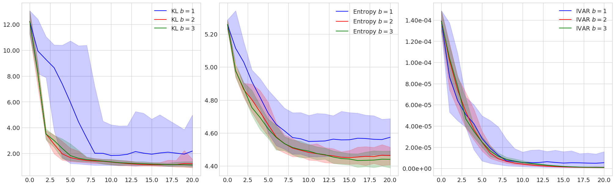
Figure 7: Influence of $b$ - Banana test case

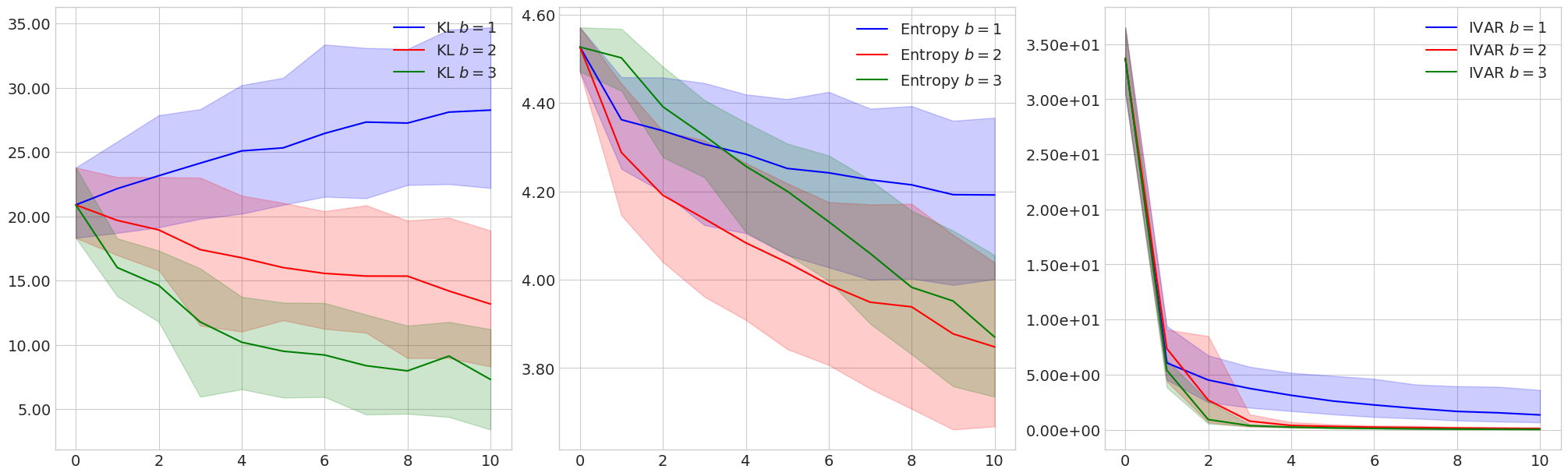
Figure 8: Influence of $b$ - Bimodal test case

One can see that for $b=1$, the design is significantly worsened. We recall that all the previous test cases where conducted with $b=3$ which provide the best results among the selected values. However, the optimal choice of $b$ is likely dependent on the application and cannot be found easily. For this reason, the IP-SUR strategy presented in this work seems superior as it does not carry the burden of an arbitrary choice of hyperparameter.
Finally, let us compare the performance of our IP-SUR method with the design strategy introduced in Sinsbeck and Nowak, (2017). The same metrics are used for comparison.

Figure 9: Comparison with Sinsbeck et al. - Banana test case

Figure 10: Comparison with Sinsbeck et al. - Bimodal test case

Figure 11: Comparison with Sinsbeck et al. - Neutronic test case

The evolution of the metrics are displayed in Figures 9, 10 and 11 for each test case. The two methods offer overall similar performance with regard to the metrics investigated, though the IP-SUR method seems more reliable for the bimodal case. Besides, it is backed by a convergence guarantee which is not the case for the method of Sinsbeck et al..

Conclusion

This work presents two new sequential design strategies to build efficient Gaussian process surrogate models in Bayesian inverse problems. These strategies are especially important for cases where the posterior distribution in the inverse problem has a thin support or is high-dimensional, in which case space-filling designs are not as competitive. The IP-SUR strategy introduced in this work is shown to be tractable and is supported by a theoretical guarantee of almost-sure convergence of the weighted integrated mean square prediction error to zero. This method is compared to a simpler CSQ strategy which is adapted from D-optimal designs and to a strategy based on the minimization of the Bayes risk with respect to the variance of the likelihood estimate. While all methods perform much better than random selection of design points, the IP-SUR method seems to provide better performance than CSQ for higher dimensions while not relying on the choice of an hyperparameter, all the while being grounded on strong theoretical foundations. It is also comparable to the Bayes risk minimzation for all test cases and even superior for the bimodal test case. The latter strategy also does not display convergence guarantee.
The IP-SUR criteria developed in this work can be related to the traditional IMSPE criteria by a tempered variant of the design strategy Neal, (2001); Hu and Zidek, (2002) in which we could introduce a $\beta\in[0,1]$ and define a new design strategy based on the functional $\mathcal{H}_{\beta}(\nu)=\int_{\mathcal{X}}k_{\nu}(\tilde{x},\tilde{x})\left(L_{\nu}(\mathbf{y}|\tilde{x})\right)^{\beta}d\tilde{x}$. The IMSPE criteria can be obtained for $\beta=0$ while the IP-SUR strategy is obtained for $\beta=1$. The supermartingale property holds for any $\beta\in[0,1]$ and the almost-sure convergence can be verified.
The extension of this design strategy is yet to be explored for other types of surrogate models. Gaussian process surrogate models have the advantage of keeping the SUR criteria tractable, though one could consider a variant to this method with approximation methods to evaluate the SUR criteria, with the risk of losing the guarantee on the convergence. The robustness of such an approach would also have to be investigated.

Appendix A Proof of supermartingale property for $\mathcal{H}$

Let us prove the supermartingale property. Let $x\in\mathcal{X}$.

$$H_{n}-J_{n}(x)=\int_{\mathcal{X}}L_{n}(\mathbf{y}|\tilde{x})k_{n}(\tilde{x},\tilde{x})F(x,\tilde{x})d\tilde{x}$$ (56)

where we introduce:

$$\begin{split}F(x,\tilde{x})=&\left[1-\left(1-\frac{\lambda_{n}(x,\tilde{x})}{k_{n}(\tilde{x},\tilde{x})}\right)\frac{|\Sigma_{n}(\tilde{x}|x)|^{1/2}}{|\Sigma_{n+1}(\tilde{x})|^{1/2}}I(\tilde{x},x)\right.\left.\frac{\exp\left(-\frac{1}{2}\left\|\mathbf{y-m_{n}}(\tilde{x})\right\|^{2}_{\Sigma_{n+1}}\right)}{\exp\left(-\frac{1}{2}\left\|\mathbf{y-m_{n}}(\tilde{x})\right\|^{2}_{\Sigma_{n}}\right)}\right]\\ \end{split}$$

Let us first show that for any $\tilde{x}\in\mathcal{X}$ we have $\left(1-\frac{\lambda_{n}(x,\tilde{x})}{k_{n}(\tilde{x},\tilde{x})}\right)\frac{|\Sigma_{n}(\tilde{x}|x)|^{1/2}}{|\Sigma_{n+1}(\tilde{x})|^{1/2}}\leq 1$. Using equation (31) one can write:

$$\left(1-\frac{\lambda_{n}(x,\tilde{x})}{k_{n}(\tilde{x},\tilde{x})}\right)\frac{|\Sigma_{n}(\tilde{x}|x)|^{1/2}}{|\Sigma_{n+1}(\tilde{x})|^{1/2}}=\left(1-\frac{\lambda_{n}(x,\tilde{x})}{k_{n}(\tilde{x},\tilde{x})}\right)\left(1-\lambda_{n}(x,\tilde{x})\|\mathbf{u}\|^{2}_{\Sigma_{n}}\right)^{-1/2}$$ (57)

Then, $0\leq\frac{\lambda_{n}(x,\tilde{x})}{k_{n}(\tilde{x},\tilde{x})}\leq 1$ and since $\|\mathbf{u}\|^{2}_{\Sigma_{n}}=\frac{N}{\sigma_{m}^{2}+Nk_{n}(\tilde{x},\tilde{x})}$ we know that $0\leq k_{n}(\tilde{x},\tilde{x})\|\mathbf{u}\|^{2}_{\Sigma_{n}}\leq 1$. Introducing this last inequality in equation (57) yields:

$$\left(1-\frac{\lambda_{n}(x,\tilde{x})}{k_{n}(\tilde{x},\tilde{x})}\right)\frac{|\Sigma_{n}(\tilde{x}|x)|^{1/2}}{|\Sigma_{n+1}(\tilde{x})|^{1/2}} =\left(1-\frac{\lambda_{n}(x,\tilde{x})}{k_{n}(\tilde{x},\tilde{x})}\right)\left(1-\frac{\lambda_{n}(x,\tilde{x})}{k_{n}(\tilde{x},\tilde{x})}\times\left(k_{n}(\tilde{x},\tilde{x})\|\mathbf{u}\|^{2}_{\Sigma_{n}}\right)\right)^{-1/2}$$

$$\leq\left(1-\frac{\lambda_{n}(x,\tilde{x})}{k_{n}(\tilde{x},\tilde{x})}\right)\left(1-\frac{\lambda_{n}(x,\tilde{x})}{k_{n}(\tilde{x},\tilde{x})}\right)^{-1/2}$$

$$=\left(1-\frac{\lambda_{n}(x,\tilde{x})}{k_{n}(\tilde{x},\tilde{x})}\right)^{1/2}\leq 1$$ (58)

The last step is to show that $I(\tilde{x},x)\exp\left(-\frac{1}{2}\left(\left\|\mathbf{y-m_{n}}(\tilde{x})\right\|^{2}_{\Sigma_{n+1}}-\left\|\mathbf{y-m_{n}}(\tilde{x})\right\|^{2}_{\Sigma_{n}}\right)\right)\leq 1$. Let us introduce $A(x,\tilde{x})$ defined by:

$$A(x,\tilde{x})=\left\|\mathbf{y-m_{n}}(\tilde{x})\right\|^{2}_{\Sigma_{n+1}}-\left\|\mathbf{y-m_{n}}(\tilde{x})\right\|^{2}_{\Sigma_{n}}+\frac{\lambda_{n}(x,\tilde{x})\left\langle\mathbf{y-m_{n}}(\tilde{x})|\mathbf{u}\right\rangle^{2}_{\Sigma_{n+1}}}{\lambda_{n}(x,\tilde{x})\|\mathbf{u}\|^{2}_{\Sigma_{n+1}}+1}$$ (59)

Then we need to show that:

$$I(\tilde{x},x)\frac{\exp\left(-\frac{1}{2}\left\|\mathbf{y-m_{n}}(\tilde{x})\right\|^{2}_{\Sigma_{n+1}}\right)}{\exp\left(-\frac{1}{2}\left\|\mathbf{y-m_{n}}(\tilde{x})\right\|^{2}_{\Sigma_{n}}\right)}=\frac{\exp\left(-\frac{1}{2}A(x,\tilde{x})\right)}{(\lambda_{n}(x,\tilde{x})\|\mathbf{u}\|^{2}_{\Sigma_{n+1}}+1)^{1/2}}\leq 1$$ (60)

Since $(\lambda_{n}(x,\tilde{x})\|\mathbf{u}\|^{2}_{\Sigma_{n+1}}+1)^{-1/2}\leq 1$ the last inequality needed is $A(x,\tilde{x})\geq 0$. Based on equation (30):

$$\Sigma_{n+1}(\tilde{x}|x)^{-1}-\Sigma_{n}(\tilde{x})^{-1}=\frac{\lambda_{n}(x,\tilde{x})}{1-\lambda_{n}(x,\tilde{x})\|\mathbf{u}\|^{2}_{\Sigma_{n}}}\Sigma_{n}(\tilde{x})^{-1}\mathbf{u}\mathbf{u}^{T}\Sigma_{n}(\tilde{x})^{-1}$$ (61)

Let us denote $B_{n}=\Sigma_{n}(\tilde{x})^{-1}\mathbf{u}\mathbf{u}^{T}\Sigma_{n}(\tilde{x})^{-1}$ and $\|a\|^{2}_{B_{n}^{-1}}=a^{T}B_{n}a$. This last notation is improper since $B_{n}$ is not invertible and its not a norm anymore since its not positive definite. It will be used for clarity purposes only. We have that:

$$\begin{split}A(x,\tilde{x})=\frac{\lambda_{n}(x,\tilde{x})}{1-\lambda_{n}(x,\tilde{x})\|\mathbf{u}\|^{2}_{\Sigma_{n}}}\|\mathbf{y-m_{n}}(\tilde{x})\|^{2}_{B_{n}^{-1}}+\frac{\lambda_{n}(x,\tilde{x})\left\langle\mathbf{y-m_{n}}(\tilde{x})|\mathbf{u}\right\rangle^{2}_{\Sigma_{n+1}}}{\lambda_{n}(x,\tilde{x})\|\mathbf{u}\|^{2}_{\Sigma_{n+1}}+1}\end{split}$$ (62)

and developing $\left\langle\mathbf{y-m_{n}}(\tilde{x})|\mathbf{u}\right\rangle^{2}_{\Sigma_{n+1}}$:

$$\begin{split}\left\langle\mathbf{y-m_{n}}(\tilde{x})|\mathbf{u}\right\rangle^{2}_{\Sigma_{n+1}}&=(\mathbf{y-m_{n}}(\tilde{x}))^{T}\Sigma_{n+1}(\tilde{x}|x)^{-1}\mathbf{u}\mathbf{u}^{T}\Sigma_{n+1}(\tilde{x}|x)^{-1}(\mathbf{y-m_{n}}(\tilde{x}))\\ &=(\mathbf{y-m_{n}}(\tilde{x}))^{T}B_{n+1}(\mathbf{y-m_{n}}(\tilde{x}))\\ &=\|\mathbf{y-m_{n}}(\tilde{x})\|^{2}_{B_{n+1}^{-1}}\end{split}$$ (63)

which yields:

$$\begin{split}A(x,\tilde{x})=&\left[(1-\lambda_{n}(x,\tilde{x})\|\mathbf{u}\|^{2}_{\Sigma_{n}})\|\mathbf{y-m_{n}}(\tilde{x})\|^{2}_{B_{n+1}^{-1}}+(1+\lambda_{n}(x,\tilde{x})\|\mathbf{u}\|^{2}_{\Sigma_{n+1}})\|\mathbf{y-m_{n}}(\tilde{x})\|^{2}_{B_{n}^{-1}}\right]\\ &\times\frac{\lambda_{n}(x,\tilde{x})}{(1-\lambda_{n}(x,\tilde{x})\|\mathbf{u}\|^{2}_{\Sigma_{n+1}})(1+\lambda_{n}(x,\tilde{x})\|\mathbf{u}\|^{2}_{\Sigma_{n}})}\\ \end{split}$$ (64)

One can show that $B_{n}=\left(\sigma_{m}^{2}+Nk_{n}(\tilde{x},\tilde{x})\right)^{-2}\mathbf{u}\mathbf{u}^{T}$. Besides $\|\mathbf{u}\|^{2}_{\Sigma_{n}}=\frac{N}{\sigma_{m}^{2}+Nk_{n}(\tilde{x},\tilde{x})}$. Then, $B_{n}=\frac{1}{N^{4}}\|u\|^{4}_{\Sigma_{n}}\mathbf{u}\mathbf{u}^{T}$. Using this relation:

$$\begin{split}A(x,\tilde{x})=&\frac{\lambda_{n}(x,\tilde{x})\left[(1-\lambda_{n}(x,\tilde{x})\|\mathbf{u}\|^{2}_{\Sigma_{n}})\|\mathbf{u}\|^{4}_{\Sigma_{n+1}}+(1+\lambda_{n}(x,\tilde{x})\|\mathbf{u}\|^{2}_{\Sigma_{n+1}})\|\mathbf{u}\|^{4}_{\Sigma_{n}}\right]}{N^{4}(1-\lambda_{n}(x,\tilde{x})\|\mathbf{u}\|^{2}_{\Sigma_{n}})(1+\lambda_{n}(x,\tilde{x})\|\mathbf{u}\|^{2}_{\Sigma_{n+1}})}\\ &\times(\mathbf{y-m_{n}}(\tilde{x}))\mathbf{u}\mathbf{u}^{T}(\mathbf{y-m_{n}}(\tilde{x}))\end{split}$$ (65)

The matrix $\mathbf{u}\mathbf{u}^{T}$ is positive non-definite and thus $(\mathbf{y-m_{n}}(\tilde{x}))\mathbf{u}\mathbf{u}^{T}(\mathbf{y-m_{n}}(\tilde{x}))\geq 0$. Besides we have shown previously that $\lambda_{n}(x,\tilde{x})\|\mathbf{u}\|^{2}_{\Sigma_{n}}\leq 1$ hence $(1-\lambda_{n}(x,\tilde{x})\|\mathbf{u}\|^{2}_{\Sigma_{n}})\geq 0$ and also $(1+\lambda_{n}(x,\tilde{x})\|\mathbf{u}\|^{2}_{\Sigma_{n+1}})\geq 0$. Let us focus on the term in between the brackets, denoted $B(x,\tilde{x})$. Using the relation $\|\mathbf{u}\|^{2}_{\Sigma_{n+1}}=\|\mathbf{u}\|^{2}_{\Sigma_{n}}\left(1-\lambda_{n}(x,\tilde{x})\|\|\mathbf{u}\|^{2}_{\Sigma_{n}}\right)^{-1}$

$$\begin{split}B(x,\tilde{x})&=\left[(1-\lambda_{n}(x,\tilde{x})\|\mathbf{u}\|^{2}_{\Sigma_{n}})\|\mathbf{u}\|^{4}_{\Sigma_{n+1}}+(1+\lambda_{n}(x,\tilde{x})\|\mathbf{u}\|^{2}_{\Sigma_{n+1}})\|\mathbf{u}\|^{4}_{\Sigma_{n}}\right]\\ &=\frac{\|\mathbf{u}\|^{4}_{\Sigma_{n}}}{1-\lambda_{n}(x,\tilde{x})\|\mathbf{u}\|^{2}_{\Sigma_{n}}}\left[1+1-\lambda_{n}(x,\tilde{x})\|\mathbf{u}\|^{2}_{\Sigma_{n}}+\lambda_{n}(x,\tilde{x})\|\mathbf{u}\|^{2}_{\Sigma_{n}}\right]\\ &=\frac{2\|\mathbf{u}\|^{4}_{\Sigma_{n}}}{1-\lambda_{n}(x,\tilde{x})\|\mathbf{u}\|^{2}_{\Sigma_{n}}}\geq 0\end{split}$$ (66)

Finally, since for all $\tilde{x}\in\mathcal{X}$, $B(x,\tilde{x})\geq 0$, then $A(x,\tilde{x})\geq 0$ and $\exp\left(-\frac{1}{2}A(x,\tilde{x})\right)\leq 1$.
Then for all $\tilde{x}\in\mathcal{X}$:

$$\left[1-\left(1-\frac{\lambda_{n}(x,\tilde{x})}{k_{n}(\tilde{x},\tilde{x})}\right)\frac{|\Sigma_{n}(\tilde{x}|x)|^{1/2}}{|\Sigma_{n+1}(\tilde{x})|^{1/2}}I(\tilde{x},x)\frac{\exp\left(-\frac{1}{2}\left\|\mathbf{y-m_{n}}(\tilde{x})\right\|^{2}_{\Sigma_{n+1}}\right)}{\exp\left(-\frac{1}{2}\left\|\mathbf{y-m_{n}}(\tilde{x})\right\|^{2}_{\Sigma_{n}}\right)}\right]\geq 0$$

which is enough to conclude that $H_{n}\geq J_{n}(x)$ for any $x\in\mathcal{X}$ based on equation (56). $H_{n}$ has the supermartingale property.
Moreover in the previous inequality, equality occurs only when $\left(1-\frac{\lambda_{n}(x,\tilde{x})}{k_{n}(\tilde{x},\tilde{x})}\right)=1$ which implies $\lambda_{n}(x,\tilde{x})=0$ and thus $k_{n}(x,\tilde{x})=0$. Or in the other hand, when $k_{n}(x,\tilde{x})=0$, then immediately $\lambda_{n}(x,\tilde{x})=0$ and $\Sigma_{n+1}(\tilde{x}|x)=\Sigma_{n}(\tilde{x})$ such that $F(x,\tilde{x})=0$. One can conclude from this, that $F(x,\tilde{x})=0$ if and only if $k_{n}(x,\tilde{x})=0$ for $x,\tilde{x}\in\mathcal{X}$.

Appendix B Proof of proposition 2.2

Let $x\in\mathcal{X}$. Consider first the total covariance matrix $\mathbf{C}_{\mathrm{tot}}(x)=v_{s}(x)\mathds{1}_{N}+\sigma_{m}^{2}\mathcal{I}_{N}$. Its inverse is given by

$$\mathbf{B}_{\mathrm{tot}}(x)=\frac{1}{\sigma_{m}^{2}}\mathcal{I}_{N}-\frac{v_{s}(x)}{\sigma_{m}^{2}(Nv_{s}(x)+\sigma_{m}^{2})}\mathds{1}_{N}$$ (67)

It is easy to verify that $\mathbf{C}_{\mathrm{tot}}(x)\mathbf{B}_{\mathrm{tot}}(x)=\mathbf{B}_{\mathrm{tot}}(x)\mathbf{C}_{\mathrm{tot}}(x)=\mathcal{I}_{N}$.
Similarly, its determinant is given by:

$$|\mathbf{C}_{\mathrm{tot}}(x)|=(\sigma_{m}^{2})^{N-1}(\sigma_{m}^{2}+Nv_{s}(x))$$ (68)

Consider now the eigenvalues $(\lambda_{j})_{1\leq j\leq N}$ of $\mathds{1}_{N}$ such that $\lambda_{1}=N$ and $\lambda_{j}=0$ for $j\geq 2$. We are interested in an orthonormal basis of eigenvectors $(e_{j})_{1\leq j\leq N}$ where $e_{j}$ is associated to the eigenvalue $\lambda_{j}$ for $1\leq j\leq N$. In particular, if $u=(1,....,1)^{T}\in\mathds{R}^{N}$, then $\mathds{1}_{N}u=Nu$ and we have $e_{1}=\frac{1}{\sqrt{N}}u$.
On this basis, we have $\mathbf{y}=\sum\limits_{j=1}^{N}c_{j}e_{j}$ where $c_{j}=\mathbf{y}^{T}e_{j}$ for $1\leq j\leq N$ by definition and $\overline{\mathbf{f_{s}}(x)}=f_{s}(x)u=\sqrt{N}f_{s}(x)e_{1}$.
Since $\mathds{1}_{N}\mathbf{y}=c_{1}\mathds{1}_{N}e_{1}=Nc_{1}e_{1}$ and $\mathds{1}_{N}\mathbf{y}=N\overline{y}u=\overline{y}N\sqrt{N}e_{1}$ with $\overline{y}=\frac{1}{N}\sum\limits_{k=1}^{N}y^{(k)}$ then $c_{1}=\sqrt{N}\overline{y}$ and $\mathbf{y}-\overline{\mathbf{f_{s}}(x)}=(\overline{y}-f_{s}(x))u+\sum\limits_{j=2}^{N}c_{j}e_{j}$. The posterior distribution can now be simplified by keeping only the term depending on $x$.
First one can see that:

$$\mathbf{C}_{\mathrm{tot}}(x)^{-1}(\mathbf{y}-\overline{\mathbf{f_{s}}(x)}) =(\overline{y}-f_{s}(x))\left(\frac{1}{\sigma_{m}^{2}}\mathcal{I}_{N}-\frac{v_{s}(x)}{\sigma_{m}^{2}(Nv_{s}(x)+\sigma_{m}^{2})}\mathds{1}_{N}\right)u+\frac{1}{\sigma_{m}^{2}}\sum\limits_{j=2}^{N}c_{j}e_{j}$$ (69)

$$=(\overline{y}-f_{s}(x))\left(\frac{1}{\sigma_{m}^{2}}-\frac{Nv_{s}(x)}{\sigma_{m}^{2}(Nv_{s}(x)+\sigma_{m}^{2})}\right)u+\frac{1}{\sigma_{m}^{2}}\sum\limits_{j=2}^{N}c_{j}e_{j}$$ (70)

since $\mathds{1}_{N}e_{j}=0$ for $j\geq 2$. Now, multiplying on the left by $(\mathbf{y}-\overline{\mathbf{f_{s}}(x)})^{T}$ and using the orthogonality of the basis vectors we have:

$$(\mathbf{y}-\overline{\mathbf{f_{s}}(x)})^{T}\mathbf{C}_{\mathrm{tot}}(x)^{-1}(\mathbf{y}-\overline{\mathbf{f_{s}}(x)})=\frac{N(\overline{y}-f_{s}(x))^{2}}{Nv_{s}(x)+\sigma_{m}^{2}}+\frac{1}{\sigma_{m}^{2}}\sum\limits_{j=2}^{N}c_{j}^{2}$$ (71)

The right term does not depend on $x$ and can be absorbed in the multiplicative constant. Finally, using equation (68) we can conclude that:

$$p(x|\mathbf{y}) \propto|\mathbf{C}_{\mathrm{tot}}(x)|^{-1/2}\exp\left[-\frac{1}{2}\left((\mathbf{y}-\overline{\mathbf{f_{s}}(x)})^{T}\mathbf{C}_{\mathrm{tot}}(x)^{-1}(\mathbf{y}-\overline{\mathbf{f_{s}}(x)})\right)\right]$$

$$\propto(\sigma_{m}^{2}+Nv_{s}(x))^{-1/2}\exp\left[-\frac{1}{2}\left(\frac{(\overline{y}-f_{s}(x))^{2}}{v_{s}(x)+\frac{\sigma_{m}^{2}}{N}}\right)\right]$$

Appendix C Extension to multi-output GP surrogates

The results presented in this paper extend naturally to multi-output Gaussian processes though for notation concision only the scalar GP case is developed. In this appendix, the formalism is extended to the multi-output case.
Let us consider $f_{s}\colon\mathcal{X}\times\Omega\xrightarrow[]{}\mathds{R}^{D}$ where $\mathcal{X}\subset\mathds{R}^{p}$ is compact. With the same notations as in section 4, the Gaussian measure conditioned by $\mathcal{F}_{n}$ is denoted $P_{n}^{f}$. The associated mean and covariance functions are $m_{n}\colon\mathcal{X}\xrightarrow[]{}\mathds{R}^{D}$ and $k_{n}\colon\mathcal{X}\times\mathcal{X}\xrightarrow[]{}M_{D}(\mathds{R})$ where $M_{D}(\mathds{R})$ is the set of squared real-valued matrices of size $D\times D$. Furthermore, for $\tilde{x}\in\mathcal{X}$ and for all $n\geq 0$, $k_{n}(\tilde{x},\tilde{x})\in S_{D}^{+}(\mathds{R})$ where $S_{D}^{+}(\mathds{R})$ is the set of symmetric positive definite matrices.
When conditioning by a input-output pair $(x,z)$, the mean and covariance functions are updated as follows:

$$m_{n+1}(\tilde{x}|x,z)=m_{n}(\tilde{x})+k_{n}(x,\tilde{x})k_{n}(x,x)^{-1}(z-m_{n}(x))$$ (72)

$$k_{n+1}(\tilde{x}_{1},\tilde{x}_{2}|x)=k_{n}(\tilde{x}_{1},\tilde{x}_{2})-k_{n}(\tilde{x}_{1},x)k_{n}(x,x)^{-1}k(x,\tilde{x}_{2})$$ (73)

Let us consider an inverse problem with observations $\mathbf{y}=(y^{(k)})_{1\leq k\leq N}$ where $y^{(k)}\in\mathds{R}^{D}$ for $1\leq k\leq N$. The observations are noisy such that:

$$y^{(k)}=f(x_{\mathrm{th}})+\varepsilon^{(k)}\text{ where }\varepsilon^{(k)}\sim\mathcal{N}\left(\mathbf{0},\mathbf{C}_{m}\right)$$ (74)

Let us introduce the total covariance $\Sigma_{n}(\tilde{x})$ for $\tilde{x}\in\mathcal{X}$.

$$\Sigma_{n}(\tilde{x})=k_{n}(\tilde{x},\tilde{x})\otimes\mathds{1}_{N}+\mathbf{C}_{m}\otimes\mathcal{I}_{N}\in\mathds{R}^{DN\times DN}$$ (75)

where $\otimes$ is the Kronecker product for matrices.
The global likelihood is the following:

$$L_{n}(\mathbf{y}|\tilde{x})=((2\pi)^{DN}|\Sigma_{n}(\tilde{x})|)^{-1/2}\exp\left[-\frac{1}{2}\left\|\mathbf{y-m_{n}}(\tilde{x})\right\|^{2}_{\Sigma_{n}}\right]$$ (76)

where the bold notation denotes the flattened vectors.

$$\mathbf{y-m_{n}}(\tilde{x})=\begin{pmatrix}y^{(1)}-m_{n}(\tilde{x})\\ \vdots\\ y^{(N)}-m_{n}(\tilde{x})\end{pmatrix}\in\mathds{R}^{DN}$$ (77)

This likelihood can be simplified in the same manner as in equation (8). The proof is not detailed here but the simplified posterior is given by:

$$p_{n}(x|\mathbf{y}) \propto\frac{1}{|\mathbf{C}_{m}+Nk_{n}(x,x)|^{1/2}}$$

$$\times\exp\left[-\frac{1}{2}\left((\overline{y}-m_{n}(x))^{T}\left(\frac{1}{N}\mathbf{C}_{m}+k_{n}(x,x)\right)^{-1}(\overline{y}-m_{n}(x))\right)\right]$$ (78)

where $\overline{y}=\frac{1}{N}\sum\limits_{k=1}^{N}y^{(k)}\in\mathds{R}^{D}$.

In this multi-output framework, the metric of uncertainty $\mathcal{H}\colon\mathds{M}\xrightarrow[]{}\mathds{R}_{+}$ is slightly different.

$$\mathcal{H}(\nu)=\int_{\mathcal{X}}|k_{\nu}(\tilde{x},\tilde{x})|L_{\nu}(\mathbf{y}|\tilde{x})d\tilde{x}$$ (79)

The SUR strategy consists in minimizing $J_{n}(x)$ defined for $x\in\mathcal{X}$ by:

$$J_{n}(x)=\mathds{E}_{z}\left[H_{n+1}(x,z)\right]=\int_{\mathcal{R}^{D}}\int_{\mathcal{X}}|k_{n+1}(\tilde{x},\tilde{x}|x)|L_{n+1}(\mathbf{y}|\tilde{x},x,z)d\tilde{x}\ \phi_{n}(z)dz$$ (80)

where $\phi_{n}(z)$ is the density of the distribution $\mathcal{N}\left(m_{n}(x),k_{n}(x,x)\right)$.
Consider a Markov chain $(X_{l})_{1\leq l\leq L}$ whose invariant distribution is the posterior $p_{n}(\tilde{x}|\mathbf{y})$. The quantity $J_{n}(x)$ can be evaluated on the Markov chain, for all $x\in\mathcal{X}$.

$$J_{n}(x)\simeq\widehat{J_{n}}(x)=\frac{1}{L}\sum\limits_{l=1}^{L}h(X_{l},x)I(X_{l},x)$$ (81)

where $h(\tilde{x},x)$ and $I(\tilde{x},x)$ are defined in the same vein as the scalar case.

$$h(\tilde{x},x)=|k_{n+1}(\tilde{x},\tilde{x})|\frac{|\Sigma_{n}(\tilde{x})|^{1/2}}{|\Sigma_{n+1}(\tilde{x}|x)|^{1/2}}\exp\left[-\frac{1}{2}\left(\left\|\mathbf{y-m_{n}}(\tilde{x})\right\|^{2}_{\Sigma_{n+1}}-\left\|\mathbf{y-m_{n}}(\tilde{x})\right\|^{2}_{\Sigma_{n}}\right)\right]$$ (82)

$$I(\tilde{x},x)=(|k_{n}(x,x)||A|)^{-1/2}\exp\left(\frac{1}{2}B^{T}A^{-1}B\right)$$ (83)

where the following notations were introduced.

$$A=k_{n}(x,x)^{-1}+k_{n}(x,x)^{-1}\mathbf{k}_{n}(\tilde{x},x)^{T}\Sigma_{n+1}(\tilde{x}|x)^{-1}\mathbf{k}_{n}(\tilde{x},x)k_{n}(x,x)^{-1}\in\mathds{R}^{D\times D}$$ (84)

$$B=k_{n}(x,x)^{-1}\mathbf{k}_{n}(\tilde{x},x)^{T}\Sigma_{n+1}(\tilde{x}|x)^{-1}(\mathbf{y-m_{n}}(\tilde{x}))\in\mathds{R}^{D}$$ (85)

$$\mathbf{k}_{n}(\tilde{x},x)=\begin{pmatrix}k_{n}(\tilde{x},x)\\ \vdots\\ k_{n}(\tilde{x},x)\end{pmatrix}\in\mathds{R}^{DN\times D}$$ (86)

Appendix D Point model approximation in neutron noise analysis

Neutron noise analysis describes a set of techniques which study the temporal fluctuations of neutron detector responses. For this particular work, the goal is to identify a fissile nuclear material based on measurements of temporal correlations between neutrons created by induced fissions inside the unknown material. From such noisy observations, an inverse problem is solved to identify the unknown material. In its simplest form, the link between material and observations is given by the so-called point model approximation, which is detailed hereafter.
The material is identified by a set of parameters $x$. In the simplest formulation of the point model, four parameters are considered such that $x\in\mathcal{X}\subset\mathds{R}^{4}$.

• $0<k_{p}<1$ is the prompt multiplication factor.

• $\varepsilon_{F}$ is the ratio of detected neutrons over the number of induced fissions in the material.

• $S$ is the source intensity in neutrons per second.

• $x_{s}$ is the ratio of source neutrons produced by spontaneous fissions, over the total number of source neutrons.

The source neutrons are either created by nuclear reactions modeled by Poisson point processes, or by spontaneous fissions which are modeled by compound Poisson processes.
The statistical model includes three different observations $y\in\mathds{R}^{3}$, which are recorded for each numerical simulations (or practical experiments).

• $R$ is the average detection rate of neutrons in the detector.

• $Y_{\infty}$ is the second order asymptotic Feynman moment.

• $X_{\infty}$ is the third order asymptotic Feynman moment.

The interpretation of the two quantities $Y_{\infty}$ and $X_{\infty}$ is not detailed here. To simplify, they can be viewed as the binomial moments of order $2$ and $3$ of the number of detected neutrons in some given time window of size $T$, where $T$ is taken to be much larger than the average lifetime of a fission chain. For more details, the authors refer to Pázsit and Pál, (2007); Furuhashi and Izumi, (1968) and Feynman et al., (1956).
In the point model framework, strong assumptions are made in order to provide an analytical link between inputs $x$ and outputs $y$. The material is assumed uniform, homogeneous and infinite. All the neutrons have same energy, and the only nuclear reactions considered are neutron captures and fissions.
In this context, analytical relations can be derived. The reactivity $\rho=\frac{k-1}{k}<0$ is introduced for concision.

$$R=-\frac{\varepsilon_{F}S\overline{\nu_{s}}}{\rho\overline{\nu}(\overline{\nu_{s}}+x_{s}-\overline{\nu_{s}}x_{s})}$$ (87)

$$Y_{\infty}=\frac{\varepsilon_{F}D_{2}}{\rho^{2}}\left(1-x_{s}\rho\frac{\overline{\nu_{s}}D_{2s}}{\overline{\nu}D_{2}}\right)$$ (88)

$$X_{\infty}=3\left(\frac{\varepsilon_{F}D_{2}}{\rho^{2}}\right)^{2}\left(1-x_{s}\rho\frac{\overline{\nu_{s}}D_{2s}}{\overline{\nu}D_{2}}\right)-\frac{\varepsilon_{F}^{2}D_{3}}{\rho^{3}}\left(1-x_{s}\rho\frac{\overline{\nu_{s}}^{2}D_{3s}}{\overline{\nu}^{2}D_{3}}\right)$$ (89)

In these relations, $\overline{\nu}$, $D_{2}$, $D_{3}$ are nuclear data quantifying the multiplicity distribution of the neutrons created by induced fissions. Similarly, $\overline{\nu_{s}}$, $D_{2s}$, $D_{3s}$ describe the multiplicity of the neutrons created by spontaneous fissions. These quantities are considered known values in this work.

References

• Agrell and Dahl, (2021) Agrell, C. and Dahl, K. R. (2021). Sequential bayesian optimal experimental design for structural reliability analysis. Statistics and Computing, 31(3):27.
• Antognini and Zagoraiou, (2010) Antognini, A. B. and Zagoraiou, M. (2010). Exact optimal designs for computer experiments via kriging metamodelling. Journal of Statistical Planning and Inference, 140(9):2607–2617.
• Azzimonti et al., (2021) Azzimonti, D., Ginsbourger, D., Chevalier, C., Bect, J., and Richet, Y. (2021). Adaptive design of experiments for conservative estimation of excursion sets. Technometrics, 63(1):13–26.
• Bect et al., (2019) Bect, J., Bachoc, F., and Ginsbourger, D. (2019). A supermartingale approach to Gaussian process based sequential design of experiments. Bernoulli, 25(4A):2883 – 2919.
• Bect et al., (2012) Bect, J., Ginsbourger, D., Li, L., Picheny, V., and Vazquez, E. (2012). Sequential design of computer experiments for the estimation of a probability of failure. Statistics and Computing, 22:773–793.
• Betancourt, (2017) Betancourt, M. (2017). A conceptual introduction to Hamiltonian Monte Carlo. arXiv preprint arXiv:1701.02434.
• Bogachev, (1998) Bogachev, V. I. (1998). Gaussian measures. American Mathematical Soc.
• Bonilla et al., (2007) Bonilla, E. V., Chai, K., and Williams, C. (2007). Multi-task gaussian process prediction. Advances in neural information processing systems, 20.
• Byrd et al., (1995) Byrd, R. H., Lu, P., Nocedal, J., and Zhu, C. (1995). A limited memory algorithm for bound constrained optimization. SIAM Journal on scientific computing, 16(5):1190–1208.
• Chevalier et al., (2014) Chevalier, C., Bect, J., Ginsbourger, D., Vazquez, E., Picheny, V., and Richet, Y. (2014). Fast parallel kriging-based stepwise uncertainty reduction with application to the identification of an excursion set. Technometrics, 56(4):455–465.
• Consonni et al., (2018) Consonni, G., Fouskakis, D., Liseo, B., and Ntzoufras, I. (2018). Prior Distributions for Objective Bayesian Analysis. Bayesian Analysis, 13(2):627 – 679.
• Dashti and Stuart, (2017) Dashti, M. and Stuart, A. M. (2017). The Bayesian Approach to Inverse Problems, pages 311–428. Springer International Publishing, Cham.
• de Aguiar et al., (1995) de Aguiar, P. F., Bourguignon, B., Khots, M., Massart, D., and Phan-Than-Luu, R. (1995). D-optimal designs. Chemometrics and intelligent laboratory systems, 30(2):199–210.
• Du and Chen, (2002) Du, X. and Chen, W. (2002). Sequential optimization and reliability assessment method for efficient probabilistic design. In International Design Engineering Technical Conferences and Computers and Information in Engineering Conference, volume 36223, pages 871–880.
• Dubourg et al., (2013) Dubourg, V., Sudret, B., and Deheeger, F. (2013). Metamodel-based importance sampling for structural reliability analysis. Probabilistic Engineering Mechanics, 33:47–57.
• Engl et al., (1996) Engl, H. W., Hanke, M., and Neubauer, A. (1996). Regularization of inverse problems, volume 375. Springer Science & Business Media.
• Ezzat et al., (2018) Ezzat, A. A., Pourhabib, A., and Ding, Y. (2018). Sequential design for functional calibration of computer models. Technometrics, 60(3):286–296.
• Feynman et al., (1956) Feynman, R. P., De Hoffmann, F., and Serber, R. (1956). Dispersion of the neutron emission in U-235 fission. Journal of Nuclear Energy (1954), 3(1-2):64–IN10.
• Frangos et al., (2010) Frangos, M., Marzouk, Y., Willcox, K., and van Bloemen Waanders, B. (2010). Surrogate and reduced-order modeling: a comparison of approaches for large-scale statistical inverse problems. Large-Scale Inverse Problems and Quantification of Uncertainty, pages 123–149.
• Furuhashi and Izumi, (1968) Furuhashi, A. and Izumi, A. (1968). Third moment of the number of neutrons detected in short time intervals. Journal of Nuclear Science and Technology, 5(2):48–59.
• Ghosh, (2011) Ghosh, M. (2011). Objective Priors: An Introduction for Frequentists. Statistical Science, 26(2):187 – 202.
• Gramacy and Lee, (2009) Gramacy, R. B. and Lee, H. K. (2009). Adaptive design and analysis of supercomputer experiments. Technometrics, 51(2):130–145.
• Hu and Zidek, (2002) Hu, F. and Zidek, J. V. (2002). The weighted likelihood. Canadian Journal of Statistics, 30(3):347–371.
• Imani and Ghoreishi, (2020) Imani, M. and Ghoreishi, S. F. (2020). Bayesian optimization objective-based experimental design. In 2020 American control conference (ACC), pages 3405–3411. IEEE.
• Jeffreys, (1946) Jeffreys, H. (1946). An invariant form for the prior probability in estimation problems. Proceedings of the Royal Society of London. Series A. Mathematical and Physical Sciences, 186(1007):453–461.
• Johnson et al., (1990) Johnson, M. E., Moore, L. M., and Ylvisaker, D. (1990). Minimax and maximin distance designs. Journal of statistical planning and inference, 26(2):131–148.
• Jones et al., (1998) Jones, D. R., Schonlau, M., and Welch, W. J. (1998). Efficient global optimization of expensive black-box functions. Journal of Global optimization, 13:455–492.
• Kaipio and Somersalo, (2006) Kaipio, J. and Somersalo, E. (2006). Statistical and computational inverse problems, volume 160. Springer Science & Business Media.
• Kennedy and O’Hagan, (2001) Kennedy, M. C. and O’Hagan, A. (2001). Bayesian calibration of computer models. Journal of the Royal Statistical Society: Series B (Statistical Methodology), 63(3):425–464.
• Kleijnen and Beers, (2004) Kleijnen, J. P. and Beers, W. V. (2004). Application-driven sequential designs for simulation experiments: Kriging metamodelling. Journal of the operational research society, 55(8):876–883.
• Kullback and Leibler, (1951) Kullback, S. and Leibler, R. A. (1951). On information and sufficiency. The annals of mathematical statistics, 22(1):79–86.
• Lartaud et al., (2023) Lartaud, P., Humbert, P., and Garnier, J. (2023). Multi-output gaussian processes for inverse uncertainty quantification in neutron noise analysis. Nuclear Science and Engineering, 197(8):1928–1951.
• Lee and Jung, (2008) Lee, T. H. and Jung, J. J. (2008). A sampling technique enhancing accuracy and efficiency of metamodel-based rbdo: Constraint boundary sampling. Computers & Structures, 86(13-14):1463–1476.
• Li and Marzouk, (2014) Li, J. and Marzouk, Y. M. (2014). Adaptive construction of surrogates for the Bayesian solution of inverse problems. SIAM Journal on Scientific Computing, 36(3):A1163–A1186.
• Mai et al., (2017) Mai, C., Konakli, K., and Sudret, B. (2017). Seismic fragility curves for structures using non-parametric representations. Frontiers of Structural and Civil Engineering, 11:169–186.
• Mitchell, (2000) Mitchell, T. J. (2000). An algorithm for the construction of “d-optimal” experimental designs. Technometrics, 42(1):48–54.
• Neal, (2001) Neal, R. M. (2001). Annealed importance sampling. Statistics and computing, 11:125–139.
• Osio and Amon, (1996) Osio, I. G. and Amon, C. H. (1996). An engineering design methodology with multistage bayesian surrogates and optimal sampling. Research in Engineering Design, 8:189–206.
• Pázsit and Pál, (2007) Pázsit, I. and Pál, L. (2007). Neutron fluctuations: A treatise on the physics of branching processes. Elsevier.
• Picheny et al., (2010) Picheny, V., Ginsbourger, D., Roustant, O., Haftka, R., and Kim, N. (2010). Adaptive designs of experiments for accurate approximation of target regions. Journal of Mechanical Design, 132.
• Ranjan et al., (2008) Ranjan, P., Bingham, D., and Michailidis, G. (2008). Sequential experiment design for contour estimation from complex computer codes. Technometrics, 50(4):527–541.
• Rasmussen and Williams, (2006) Rasmussen, C. E. and Williams, C. K. I. (2006). Gaussian processes for machine learning. MIT Press.
• Sacks et al., (1989) Sacks, J., Schiller, S. B., and Welch, W. J. (1989). Designs for computer experiments. Technometrics, 31(1):41–47.
• Salvatier et al., (2016) Salvatier, J., Wiecki, T. V., and Fonnesbeck, C. (2016). Probabilistic programming in python using pymc3. PeerJ Computer Science, 2:e55.
• Santner et al., (2003) Santner, T. J., Williams, B. J., Notz, W. I., and Williams, B. J. (2003). The design and analysis of computer experiments, volume 1. Springer.
• Scales and Tenorio, (2001) Scales, J. A. and Tenorio, L. (2001). Prior information and uncertainty in inverse problems. Geophysics, 66(2):389–397.
• Schobi et al., (2015) Schobi, R., Sudret, B., and Wiart, J. (2015). Polynomial-chaos-based kriging. International Journal for Uncertainty Quantification, 5(2).
• Shahriari et al., (2015) Shahriari, B., Swersky, K., Wang, Z., Adams, R. P., and De Freitas, N. (2015). Taking the human out of the loop: A review of Bayesian optimization. Proceedings of the IEEE, 104(1):148–175.
• Shewry and Wynn, (1987) Shewry, M. C. and Wynn, H. P. (1987). Maximum entropy sampling. Journal of applied statistics, 14(2):165–170.
• Sinsbeck et al., (2021) Sinsbeck, M., Cooke, E., and Nowak, W. (2021). Sequential design of computer experiments for the computation of bayesian model evidence. SIAM/ASA Journal on Uncertainty Quantification, 9(1):260–279.
• Sinsbeck and Nowak, (2017) Sinsbeck, M. and Nowak, W. (2017). Sequential design of computer experiments for the solution of bayesian inverse problems. SIAM/ASA Journal on Uncertainty Quantification, 5(1):640–664.
• Snoek et al., (2012) Snoek, J., Larochelle, H., and Adams, R. P. (2012). Practical Bayesian optimization of machine learning algorithms. Advances in neural information processing systems, 25.
• Stein, (1987) Stein, M. (1987). Large sample properties of simulations using latin hypercube sampling. Technometrics, 29(2):143–151.
• Stroh et al., (2022) Stroh, R., Bect, J., Demeyer, S., Fischer, N., Marquis, D., and Vazquez, E. (2022). Sequential design of multi-fidelity computer experiments: maximizing the rate of stepwise uncertainty reduction. Technometrics, 64(2):199–209.
• Stuart, (2010) Stuart, A. M. (2010). Inverse problems: a bayesian perspective. Acta numerica, 19:451–559.
• Sürer et al., (2023) Sürer, Ö., Plumlee, M., and Wild, S. M. (2023). Sequential bayesian experimental design for calibration of expensive simulation models. Technometrics, 0(ja):1–26.
• Vakhania et al., (1987) Vakhania, N., Tarieladze, V., and Chobanyan, S. (1987). Probability distributions on Banach spaces, volume 14. Springer Science & Business Media.
• van der Vaart et al., (2008) van der Vaart, A. W., van Zanten, J. H., et al. (2008). Reproducing kernel hilbert spaces of gaussian priors. IMS Collections, 3:200–222.
• Villemonteix et al., (2009) Villemonteix, J., Vazquez, E., and Walter, E. (2009). An informational approach to the global optimization of expensive-to-evaluate functions. Journal of Global Optimization, 44:509–534.
• Wang et al., (2006) Wang, Y., Myers, R. H., Smith, E. P., and Ye, K. (2006). D-optimal designs for poisson regression models. Journal of statistical planning and inference, 136(8):2831–2845.
• Xiang et al., (1997) Xiang, Y., Sun, D., Fan, W., and Gong, X. (1997). Generalized simulated annealing algorithm and its application to the thomson model. Physics Letters A, 233(3):216–220.
• Zhang et al., (2019) Zhang, R., Lin, C. D., and Ranjan, P. (2019). A sequential design approach for calibrating dynamic computer simulators. SIAM/ASA Journal on Uncertainty Quantification, 7(4):1245–1274.