Periodically driven thermodynamic systems under vanishingly small viscous drives

Abstract

Periodically driven thermodynamic systems support stable non-equilibrium oscillating states with properties drastically different from equilibrium. They exhibit even more exotic features for low viscous drives, which is a regime that is hard to probe due to singular behavior of the underlying Langevin dynamics near vanishing viscosity. We propose a method, based on singular perturbation and Floquet theories, that allows us to obtain oscillating states in this limit. We then find two distinct classes of distributions, each exhibiting interesting features that can be exploited for a range of practical applicability, including cooling a system and triggering chemical reactions through weakly interacting driven environments.

Introduction.– Langevin framework provides a simple and suitable description for periodically driven thermodynamic systems and allows us to effectively probe their properties beyond equilibrium [1, 2, 3]. It is therefore not surprising to witness the current proliferation of studies on periodically driven Langevin systems knowing their relevance not only for thermodynamic systems like heat engines [4, 5, 6, 7] and nano-mechanical resonators [8, 9, 10] but also for wider range of applications including climate modeling [11, 12, 13, 14, 15], biological processes [16, 17] and ecological trends [18, 19, 20].

In this Letter, we focus our study, for multiple reasons, on a periodically driven under-damped Brownian particle moving in small viscous regime. Firstly, Brownian particle is a paradigmatic Langevin system that can aid in extracting general nonequilibrium features of macroscopic systems [2, 1]. Secondly, inertial effects can become significant with increasing drive frequency. Thirdly, driven Brownian particle is known to exist in stable nonequilibrium states including oscillating states [21, 22, 23, 24, 25]. Fourthly, the limit of vanishing viscosity is singular and of immense interest both for mathematical and physical reasons, including in the study of inviscid flows [26, 27, 28] and in understanding the eluding turbulence [29, 30].

Periodically driven Langevin systems do not relax to equilibrium, and instead can support non-equilibrium states, referred to as oscillating states (OS) [22, 23, 24, 25, 31, 32]. Unlike in equilibrium, for a given bath temperature OS are not independent of viscosity and can carry significant viscous memory and in turn exhibit drastically distinct thermodynamic properties. Though the effects of viscosity in various stochastic systems are extensively studied over the whole gamut [33, 34], there is in general a bias towards large viscous or over-damped regimes [35, 36, 37, 38]. The systems typically relax fast in this regime and are easy to control, numerically or perturbatively, their convergence to the asymptotic state. Furthermore their dynamics usually reduce to mathematically well-studied continuous Markov processes. But the physics exhibited by Langevin systems when viscosity is small [39, 40, 28, 41] can be antithetical to that when it is large, particularly in the presence of drives where inertial effects do not decouple, and thus obligates dedicated study. This motivates us to address and answer the questions: How do we identify an oscillating state (OS) when the approach to asymptotic state becomes increasingly sluggish as viscosity reduces? What are the properties of OS, if they exist, in this singular limit of vanishing viscosity? Is it possible to develop a systematic perturbative scheme about the singular limit? How distinct are low viscous OS? What novel mechanisms and applications can their study lead us to?

Model.–We consider a Brownian particle in harmonic potential described by an under-damped Langevin equation

$$\dot{X}_{t}=V_{t}~{},\quad\dot{V}_{t}=-\gamma(t)V_{t}-k_{0}X_{t}+\eta(t)~{},$$ (1)

where $-k_{0}X_{t}$ denotes the external force parameterized by$~{}k_{0}$. The particle experiences$~{}-\gamma(t)V_{t}$ viscous drag and a random Gaussian noise$~{}\eta(t)$ with zero mean and $\langle\eta_{t}\eta_{t^{\prime}}\rangle=2D(t)\delta(t-t^{\prime})$. We choose$~{}k_{0}$ to be constant while$~{}\gamma(t)$ and$~{}D(t)$ are time-dependent functions with period$~{}T$.

In order to investigate the influence of drives on asymptotic states in low viscous regime, we extend the chosen periodic functions $\gamma(t)\to\gamma_{\alpha}(t)=\alpha\gamma(t)$ and $D(t)\to D_{\alpha}(t)=\alpha D(t)$ by a one-parameter extension labeled by a real positive number$~{}\alpha$. This extension keeps the bath temperature $T_{b}(t)~{}=~{}D(t)/\gamma(t)$ independent of$~{}\alpha$, and has the advantage of isolating the dependence of these non-equilibrium states on viscous drives$~{}\gamma_{\alpha}(t)$ for given$~{}T_{b}(t)$. We aim to first find the asymptotic states in the limit$~{}\alpha\to 0$, and then explore their properties in the neighborhood of$~{}\alpha=0$.

The distribution $P(x,v,t)$ associated with the random process in Eq. (1), satisfies the Fokker-Planck (FP) equation given by

$$\frac{\partial}{\partial t}P(x,v,t)=\mathscr{L}(x,v;g(t))P(x,v,t)~{},$$ (2)

where $g$ denotes all the parameters, including $\gamma$ and $D$, and the FP operator $\mathscr{L}$ is defined as

$$\mathscr{L}(x,v;g):=-\frac{\partial}{\partial x}v-\frac{\partial}{\partial v}\left[-\gamma_{\alpha}v-k_{0}x\right]+D_{\alpha}\frac{\partial^{2}}{\partial v^{2}}~{}.$$ (3)

Under certain conditions [24, 25], $P(x,v,t)$ at large times takes a time periodic form which is independent of the initial conditions. These distributions of asymptotic states, also referred to as OS, are denoted by $P_{os}(x,v,t)$ and defined as

$$P_{\text{os}}(x,v,t):=\lim_{N\to\infty}P(x,v,NT+t)~{}.$$ (4)

The choice of harmonic potential$~{}k_{0}x^{2}/2$ is not a restriction. The method we propose to find OS and the general results that follow thereafter are equally applicable to any (driven) polynomial potentials $U(x;\lambda(t))=\sum_{n}\lambda_{n}(t)x^{n}$.

Method.–The OS distribution for given $\alpha$ has a perturbative expansion

$$P_{\text{os}}(t;\alpha)=P_{\text{os}}^{(0)}(t)+\alpha P_{\text{os}}^{(1)}(t)+\alpha^{2}P_{\text{os}}^{(2)}(t)+\cdots~{},$$ (5)

where $x,v$ dependence is not shown explicitly for convenience. The standard procedure of obtaining perturbative solution $P(t;\alpha)=\sum_{n=0}^{\infty}\alpha^{n}P^{(n)}(t)$ amounts to solving the hierarchy of equations

$$\frac{\partial}{\partial t}P^{(n)}(t)=\mathscr{L}_{0}P^{(n)}(t)+\mathscr{L}_{1}P^{(n-1)}(t)~{},$$ (6)

where $P^{(-1)}(t)=0$, the Liouville operator$~{}\mathscr{L}_{0}$ and perturbative operator$~{}\mathscr{L}_{1}$ are the $O(1)$ and $O(\alpha)$ parts of the FP operator, respectively. The Liouville equation is a singular limit of FP equation and its solution, which has no large-time limit, depends on the initial condition. Hence the hierarchy of solutions of Eqs. (6) depend on their initial conditions$~{}P_{in}^{(m)}$ and result in the full solution

$$P(t;\alpha)=\sum_{n=0}^{\infty}\alpha^{n}P^{(n)}(t;\{P_{in}^{(m)}\}_{m\leq n})~{},$$ (7)

which asymptotically will not coincide with$~{}P_{\text{os}}(t;\alpha)$. This is expected since the limits $\alpha\to 0$ and $t\to\infty$ do not commute in this singular perturbation problem. Instead we employ Floquet theory to obtain the OS distribution for finite$~{}\alpha$ wherein we impose periodicity on$~{}P(t;\alpha)$ and in turn determine the hierarchy of initial conditions$~{}\{P_{in}^{(m)}\}$ uniquely. This uniqueness is ensured since OS is unique, periodic and independent of the full initial condition. We need to impose periodicity to$~{}O(\alpha^{n+1})$ in order to determine$~{}\{P_{in}^{(m)}\}$ to$~{}O(\alpha^{n})$.

The distribution can also be obtained from its moments which satisfy ordinary differential equations. This does not mean the hurdles of singular limit can be avoided, but can be handled following the proposed method as detailed in the supplemental materials (SM) [42].

Results.–The OS of harmonic Brownian particle is Gaussian [24] with zero mean and time-periodic covariance matrix$~{}\Sigma$ whose elements are second moments $\Sigma_{11}=\left\langle x^{2}\right\rangle$, $\Sigma_{12}=\Sigma_{21}=\langle xv\rangle$ and $\Sigma_{22}=\left\langle v^{2}\right\rangle$.

We have established that the condition $k_{0}>0$ is sufficient to ensure the existence of OS in the small $\alpha$ regime for any bounded positive real periodic functions $\gamma(t)$ and $D(t)$ of time-period $T=2\pi/\omega$. In fact, we can specify an implicit inequality given$~{}\gamma(t)$ and$~{}k_{0}$ (or$~{}k(t)$, a time-dependent harmonic drive) that is necessary to satisfy for the existence of OS, as specified in SM [42].

The existence of OS implies that the proposed perturbative method can be employed to obtain its distribution. We find two distinct classes of distributions having differing statistical behavior at the leading order which is a consequence of whether the time scales associated with potential and drive are in tune or not. They are distinguished by whether at least one of the drives$~{}\gamma$ or $D$ contains any harmonic $n_{0}\omega=\pm 2\sqrt{k_{0}}$ or not.

Case I: When the potential strength$~{}k_{0}\neq n_{0}^{2}\omega^{2}/4$, for all integers$~{}n_{0}$, then we find the leading-order moments of OS to be

$$\Sigma_{11}^{(0)}=\frac{1}{k_{0}}\frac{\overline{D}}{\overline{\gamma}}~{},\quad\Sigma_{12}^{(0)}=0~{},\quad\Sigma_{22}^{(0)}=\frac{\overline{D}}{\overline{\gamma}}~{},$$ (8)

where the overline denotes time average over a period. Thus OS distributions in the limit $\alpha\to 0$ are time-independent and depend only on time-averaged viscous and noise parameters. It does not mean that viscous drive has no effect for given time-dependent bath temperature since $\overline{D}=\overline{\gamma T_{b}}$. The time dependence and periodicity of OS are seen at the next-order. The explicit expressions of moments to first-order and their numerical verification are given in SM [42].

We see that in general the kinetic temperature $T_{s}(t):=\Sigma_{22}(t)$ of the particle in OS differs from bath-temperature $T_{b}(t)$ and its correlation function$~{}\Sigma_{12}(t)$ is non-zero. Though these observables distinguish OS from equilibrium, there are other non-equilibrium variables, such as house-keeping heat flux, entropy flux and entropy production, whose relevance is evident when we view OS as a cyclic process governed by stochastic thermodynamics.

In an infinitesimal time $dt$ of the cyclic process, at the level of an individual Langevin trajectory the change in energy $dE_{t}=d\bar{}\hskip 1.00006ptQ+d\bar{}\hskip 1.00006ptW$ [43]. The work done on the particle $d\bar{}\hskip 1.00006ptW:=\dot{g}\cdot\partial_{g}E_{t}dt$ depends on periodic drives$~{}g(t)$ and thus vanishes in absence of potential drive. The heat received from the bath is $d\bar{}\hskip 1.00006ptQ_{t}:=-\gamma V_{t}^{2}dt+V_{t}\circ dB_{t}$, where ${dB_{t}=\int_{t}^{t+dt}dt^{\prime}\eta(t^{\prime})}$ is the Brownian noise and $\circ$ denotes Stratonovich product. We find the rate of heat dissipation

$$q_{\text{hk}}=-\frac{\langle d\bar{}\hskip 1.00006ptQ_{t}\rangle}{dt} =\gamma_{\alpha}\langle V_{t}^{2}\rangle-D_{\alpha}=\alpha\gamma\left(T_{s}-T_{b}\right),$$ (9)

linearly depends on instantaneous difference of the two temperatures. This dissipation is indispensable to maintain the particle in given OS and hence is referred to as house-keeping heat flux. The Langevin dynamics also determines the rate of change of entropy

$$\frac{dS}{dt}=\frac{\gamma_{\alpha}}{D_{\alpha}}\frac{\langle d\bar{}\hskip 1.00006ptQ_{t}\rangle}{dt}+\frac{1}{D_{\alpha}}\left\langle\left(\frac{\hat{J}_{v}^{\text{ir}}}{\hat{P}_{\text{os}}}\right)^{2}_{t}\right\rangle~{},$$ (10)

where $S$  $=\langle-\log\hat{P}_{os}\rangle$ [44] and the stochastic variables $\hat{P}_{os}=P_{os}(X_{t},V_{t},t)$ and $\hat{J}_{v}^{\text{ir}}=J_{v}^{\text{ir}}(X_{t},V_{t},t)$ are associated with $P_{os}(x,v,t)$ and the irreversible part of probability current $J_{v}^{\text{ir}}(x,v,t)=-\left(\gamma_{\alpha}v+D_{\alpha}\partial_{v}\right)P_{\text{os}}(x,v,t)~{}.$ Eq. (10) not only confirms the asserted bath-temperature $T_{b}=D/\gamma$ but also enables us to identify house-keeping entropy flux

$$\Phi_{\text{hk}} :=\frac{q_{\text{hk}}}{T_{b}}=-\alpha\gamma\left(1-\frac{1}{T_{b}}\frac{\overline{D}}{\overline{\gamma}}\right)+\cdots~{},$$ (11)

and house-keeping entropy production

$$\Pi_{\text{hk}}:=\frac{1}{D_{\alpha}}\left\langle\left(\frac{\hat{J}_{v}^{\text{ir}}}{\hat{P}_{\text{os}}}\right)^{2}_{t}\right\rangle=\frac{\alpha}{D}\left(\sqrt{\frac{\overline{D}}{\overline{\gamma}}}\gamma-\sqrt{\frac{\overline{\gamma}}{\overline{D}}}D\right)^{2}+\cdots~{}.$$ (12)

The expression $\dot{S}=\Pi_{\text{hk}}-\Phi_{\text{hk}}$ implies that entropy flux and its production are not equal in OS, unlike in steady state, but their time-period averages are. The cyclic process viewpoint thus provides the physical picture where OS is sustained due to a dynamical interplay between entropy production in the system and heat exchange with the bath.

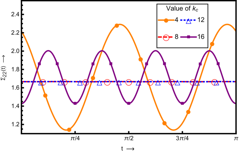
Figure 1: The asymptotic value of $\Sigma_{22}(t)$ have been plotted for different values of potential parameter $k_{0}$. The viscous coefficient $\gamma(t)=3+\sin(\omega t)+\cos(2\omega t)$, noise strength $D(t)=5+3\cos(\omega t)$, drive frequency $\omega=4$ and $\alpha=0.001$.

In the leading order, we see that $P_{\text{os}}$ is time independent, its irreversible current is identically zero, the fluxes vanish and the entropy production rate is nil. The necessary and sufficient conditions for detailed balance [45, 46, 47, 48] are thus satisfied, and the distribution is à la Boltzmann with an effective temperature $T_{s}^{(0)}=\overline{D}/\overline{\gamma}$. This is in contrast with $\alpha\rightarrow\infty$ case where the limiting distribution is far from equilibrium in spite of zero entropy production rate [31]. While OS tends to equilibrium when $\alpha\rightarrow 0$, the effective temperature is neither instantaneous bath-temperature nor its time average. For instance, the analytically solvable choice $D=D_{0}+D_{1}\cos(\omega t)$ and $\gamma=\gamma_{0}+\gamma_{1}\cos(\omega t)$ leads to the relation

$$\overline{T}_{b}-\frac{D_{1}}{\gamma_{1}}=\frac{\gamma_{0}}{\sqrt{\gamma_{0}^{2}-\gamma_{1}^{2}}}\left(T_{s}^{(0)}-\frac{D_{1}}{\gamma_{1}}\right)~{},$$ (13)

which implies that the effective temperature can be greater or lesser than $\overline{T}_{b}$. If both $\overline{T}_{b}$ and $T_{s}^{(0)}$ are greater (lesser) than $D_{1}/\gamma_{1}$, then $T_{s}^{(0)}$ is lesser (greater) than $\overline{T}_{b}$.

The results also suggest a mechanism to cool (or heat) a system with the help of a weakly interacting driven bath. Furthermore, they indicate, for instance, the possibility of maintaining a steady temperature indoors that keeps you cooler during day and warmer at night without consuming extra electricity [49].

Case II: When $k_{0}=n_{0}^{2}\omega^{2}/4$ for some non-zero integer$~{}n_{0}$, we observe numerically that OS show significant time dependence at small $\alpha$ limit, and hence will be referred to as resonant states. We plot as an example, the moment $\Sigma_{11}(t)$ in Fig. 1 for the choice $\gamma(t)=3+\sin(\omega t)+\cos(2\omega t)$, $D(t)=5+3\cos(\omega t)$, $\omega=4$ and $\alpha=0.001$. We observe that the resonant states occur only when $k_{0}=4\text{ or }16$, namely $k_{0}=4n_{0}^{2}$, where $n_{0}=1\text{ or }2$ and are the only harmonics present in $\gamma$ or $D$.

The proposed perturbative method enables us to find analytically the moments of resonating states and explain the observed peculiarities. It is convenient to separate the constant term and $n_{0}$-th harmonic, where $n_{0}$ satisfies $k_{0}=n_{0}^{2}\omega^{2}/4$, and decompose the functions as

$$\gamma(t)= \gamma_{0}+\gamma_{+}e^{-in_{0}\omega t}+\gamma_{-}e^{in_{0}\omega t}+\gamma^{\prime}(t)~{},$$ (14)

$$D(t)= D_{0}+D_{+}e^{-in_{0}\omega t}+D_{-}e^{in_{0}\omega t}+D^{\prime}(t)~{},$$ (15)

where constants $\gamma_{0}$ and $D_{0}$ are real, $n_{0}$-th Fourier coefficients satisfy $\gamma_{\pm}=\gamma_{\mp}^{*}$ and $D_{\pm}=D_{\mp}^{*}$, and $\gamma^{\prime}(t)$ and $D^{\prime}(t)$ contain remaining modes. We find the leading-order moments to be

$$\Sigma_{11}^{(0)} =C_{-}^{(0)}e^{in_{0}\omega t}+C_{0}^{(0)}+C_{+}^{(0)}e^{-in_{0}\omega t}~{},$$ (16)

$$\Sigma_{12}^{(0)} =\frac{i}{2}n_{0}\omega\left(C_{-}^{(0)}e^{in_{0}\omega t}-C_{+}^{(0)}e^{-in_{0}\omega t}\right)~{},$$ (17)

$$\Sigma_{22}^{(0)} =-\frac{n_{0}^{2}\omega^{2}}{4}\left(C_{-}^{(0)}e^{in_{0}\omega t}-C_{0}^{(0)}+C_{+}^{(0)}e^{-in_{0}\omega t}\right),$$ (18)

where

$$C_{\pm}^{(0)}= -\frac{2D_{\pm}}{n_{0}^{2}\omega^{2}\gamma_{0}}+\frac{C_{0}^{(0)}\gamma_{\pm}}{2\gamma_{0}}~{},$$ (19)

$$C_{0}^{(0)}= \frac{4D_{0}\gamma_{0}-2\left(D_{+}\gamma_{-}+D_{-}\gamma_{+}\right)}{n_{0}^{2}\omega^{2}\left(\gamma_{0}^{2}-\gamma_{+}\gamma_{-}\right)}~{}.$$ (20)

We see that the moments are time-dependent even in $\alpha\to 0$ limit and depend not only on time-averaged drives but also $n_{0}$-th Fourier components. If both $\gamma$ and $D$ do not contain $n_{0}$-th harmonic, OS belongs to Case I. The amplitudes of $\Sigma_{11}$ and $\Sigma_{12}$ decrease with increasing $n_{0}$, a trend noticed earlier in Fig. 1. Interestingly, we further find that the time-period of OS at leading order is $T/n_{0}$. The result suggests a mechanism to activate a system in a higher-harmonic mode of the weakly interacting bath, and may have immense potential for pragmatic utility. Furthermore, we provide the moments to first-order and their numerical verification in SM [42]. We note that the first-order corrections revert the periodicity of OS back to drive period$~{}T$.

In spite of resonant states being time-dependent in the limit $\alpha\to 0$, we find as in Case I that the work done, the irreversible current, the house-keeping fluxes and entropy production in OS vanish. Hence the system in resonant OS is also energetically isolated with constant energy$~{}E$. We find $E=2k_{0}C_{0}^{(0)}$, where $C_{0}^{(0)}$ is given by Eq. (20), though both kinetic energy$~{}\langle E_{k}\rangle=\Sigma_{22}/2$ and potential energy $\langle U\rangle=k_{0}\Sigma_{11}/2$ are time dependent. Both change in synchrony by keeping the sum $\langle E_{k}\rangle+\langle U\rangle$ fixed, which can be verified explicitly using Eqs. (16, 18). While it may be hard to imagine an isolated system being in a time-dependent state, it does so by a perpetual exchange of energy between its position and velocity degrees of freedom. The maneuver of this exchange is encoded in the correlation function$~{}\Sigma_{12}$ given by Eq. (17).

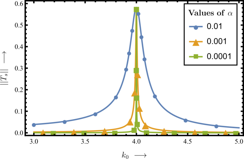
Figure 2: The amplitudes of oscillations of the system temperature $||T_{s}(t)||$ have been plotted for different values of potential parameter $k_{0}$. The viscous coefficient $\gamma(t)=3+\sin(\omega t)+\cos(2\omega t)$, noise strength $D(t)=5+3\cos(\omega t)$, drive frequency $\omega=4$ and $\alpha=\{0.01,0.001,0.0001\}$.

Since resonant states emerge at fine-tuned condition, it may appear that they are impractical to realize, sustain and manipulate experimentally. The first-order corrections $\Sigma_{ij}^{(1)}$ in fact tell us that when $k_{0}$ deviates from $n_{0}^{2}\omega^{2}/4$ by an amount $\Delta k\ll n_{0}\omega^{2}$, then the contribution from $n_{0}$-th mode of the drives dominates over the rest. Thus operating the system at small non-zero $\alpha$, either by design or due to inevitable influence of the bath, is sufficient to maintain it in an OS showing features of resonant states. To illustrate the non-equilibrium behavior in the vicinity of resonant points for small$~{}\alpha$, we plot in Fig. 2 the amplitude of oscillating system temperature$~{}T_{s}$ as we sweep$~{}k_{0}$, for the choice $\gamma(t)=3+\sin(\omega t)+\cos(2\omega t)$, $D(t)=5+3\cos(\omega t)$ and $\omega=4$. The amplitude dies down as $k_{0}$ deviates from $4$, thus signaling equilibrium. Moreover, the range of non-equilibrium behavior sharply falls off with decreasing$~{}\alpha$.

The OS behavior in the limit $\alpha\to 0$ that we report is not restricted to harmonic potential alone. Both equilibrium and resonant limits continue to exhibit the same qualitative features when time-independent anharmonic terms are added. The resonant condition gets modified and can be systematically evaluated in anharmonic expansion. When either harmonic or anharmonic terms become time dependent, then the leading behavior is no longer equilibrium even in the generic case. The proposed perturbative method though can be employed to analyze all these cases as detailed in the SM [42].

Conclusions.–Low viscous physics of Langevin systems is relatively difficult to probe due to slow convergence and the singular nature of the limit. We have proposed a method based on singular perturbation and Floquet theories that is suitable to determine OS distributions of driven Langevin systems for low viscous drives. The proposed method is extensively verified with exact numerical calculations and simulations for determining OS of a driven under-damped Brownian particle moving in one-dimensional space in harmonic and quartic (driven) potentials. The method is in principle applicable to any driven (interacting multi-particle) Langevin systems non-perturbatively or to any order of perturbation. It can also be extended to Floquet quantum systems.

We find that the low viscous OS fall into two classes, distinguishable by a resonance condition, each with strikingly different physical features. In vanishing viscosity limit, OS belonging to the generic class tends to an equilibrium state with an effective temperature that can be tuned by viscous and thermal drives. This feature can be expected even in interacting systems and thus opening up possibilities for practical applications including cooling a system using a periodic time-dependent environment. For the fine-tuned class, when viscosity vanishes and the system is isolated from its environment, the OS continue to exhibit non-equilibrium properties where internal degrees resonate with one other in fractional time-period. This feature, expected to show up in interacting systems around fine-tuned parameters of the potentials, is indeed promising for various applications including higher harmonic activation [50, 51]. It would be interesting to come up with drive protocols for the environment to engineer resonant OS on systems (for example nano-robots [52]) required for some specific purpose.

References

- Van Kampen [1992] N. G. Van Kampen, Stochastic Processes in Physics and Chemistry, Vol. 1 (Elsevier, 1992).
- Risken [1996] H. Risken, The Fokker-Planck Equation (Springer-Verlag Berlin Heidelberg, 1996).
- Zinn-Justin [2021] J. Zinn-Justin, Quantum field theory and critical phenomena, Vol. 171 (Oxford university press, 2021).
- Quinto-Su [2014] P. A. Quinto-Su, A microscopic steam engine implemented in an optical tweezer, Nature communications 5, 5889 (2014).
- Martínez et al. [2017] I. A. Martínez, É. Roldán, L. Dinis, and R. A. Rica, Colloidal heat engines: a review, Soft matter 13 (2017).
- Pietzonka and Seifert [2018] P. Pietzonka and U. Seifert, Universal trade-off between power, efficiency, and constancy in steady-state heat engines, Phys. Rev. Lett. 120, 190602 (2018).
- Lu et al. [2022] J. Lu, Z. Wang, J. Peng, C. Wang, J.-H. Jiang, and J. Ren, Geometric thermodynamic uncertainty relation in a periodically driven thermoelectric heat engine, Phys. Rev. B 105, 115428 (2022).
- Cleland and Roukes [2002] A. Cleland and M. Roukes, Noise processes in nanomechanical resonators, Journal of applied physics 92, 2758 (2002).
- Unterreithmeier et al. [2010] Q. P. Unterreithmeier, T. Faust, and J. P. Kotthaus, Damping of nanomechanical resonators, Phys. Rev. Lett. 105, 027205 (2010).
- Eom et al. [2011] K. Eom, H. S. Park, D. S. Yoon, and T. Kwon, Nanomechanical resonators and their applications in biological/chemical detection: Nanomechanics principles, Physics Reports 503, 115 (2011).
- Palmer [2019] T. Palmer, Stochastic weather and climate models, Nature Reviews Physics 1, 463 (2019).
- Margazoglou et al. [2021] G. Margazoglou, T. Grafke, A. Laio, and V. Lucarini, Dynamical landscape and multistability of a climate model, Proceedings of the Royal Society A 477, 20210019 (2021).
- Held [1982] I. M. Held, Climate models and the astronomical theory of the ice ages, Icarus 50, 449 (1982).
- Wiesenfeld and Moss [1995] K. Wiesenfeld and F. Moss, Stochastic resonance and the benefits of noise: from ice ages to crayfish and squids, Nature 373, 33 (1995).
- Lucarini [2019] V. Lucarini, Stochastic resonance for nonequilibrium systems, Phys. Rev. E 100, 062124 (2019).
- Schmiedl et al. [2007] T. Schmiedl, T. Speck, and U. Seifert, Entropy production for mechanically or chemically driven biomolecules, Journal of Statistical Physics 128, 77 (2007).
- Jain and Kaushik [2022] K. Jain and S. Kaushik, Joint effect of changing selection and demography on the site frequency spectrum, Theoretical Population Biology 146, 46 (2022).
- Kuehn and Gross [2013] C. Kuehn and T. Gross, Nonlocal generalized models of predator-prey systems, Discrete and Continuous Dynamical Systems - B 18, 693 (2013).
- Rozenfeld et al. [2001] A. F. Rozenfeld, C. J. Tessone, E. Albano, and H. S. Wio, On the influence of noise on the critical and oscillatory behavior of a predator–prey model: coherent stochastic resonance at the proper frequency of the system, Physics Letters A 280, 45 (2001).
- Ma et al. [2023] H.-Y. Ma, C. Liu, Z.-X. Wu, and J.-Y. Guan, Periodic environmental effect: stochastic resonance in evolutionary games of rock-paper-scissors, Physica Scripta 98, 065210 (2023).
- Jung [1993] P. Jung, Periodically driven stochastic systems, Physics Reports 234, 175 (1993).
- Koyuk and Seifert [2019] T. Koyuk and U. Seifert, Operationally accessible bounds on fluctuations and entropy production in periodically driven systems, Phys. Rev. Lett. 122, 230601 (2019).
- Proesmans et al. [2016] K. Proesmans, B. Cleuren, and C. Van den Broeck, Linear stochastic thermodynamics for periodically driven systems, Journal of Statistical Mechanics: Theory and Experiment 2016, 023202 (2016).
- Awasthi and Dutta [2020] S. Awasthi and S. B. Dutta, Periodically driven harmonic langevin systems, Phys. Rev. E 101, 042106 (2020).
- Awasthi and Dutta [2021] S. Awasthi and S. B. Dutta, Oscillating states of periodically driven anharmonic langevin systems, Phys. Rev. E 103, 062143 (2021).
- Ludford [1960] G. S. S. Ludford, Inviscid flow past a body at low magnetic reynolds number, Rev. Mod. Phys. 32, 1000 (1960).
- Friedlander and Vishik [1991] S. Friedlander and M. M. Vishik, Instability criteria for the flow of an inviscid incompressible fluid, Phys. Rev. Lett. 66, 2204 (1991).
- Prakash et al. [2013] J. Prakash, O. M. Lavrenteva, and A. Nir, Interaction of bubbles in an inviscid and low-viscosity shear flow, Phys. Rev. E 88, 023021 (2013).
- Sreenivasan [1999] K. R. Sreenivasan, Fluid turbulence, Rev. Mod. Phys. 71, S383 (1999).
- Campbell and Turner [1985] I. Campbell and J. Turner, Turbulent mixing between fluids with different viscosities, Nature 313, 39 (1985).
- Awasthi and Dutta [2022] S. Awasthi and S. B. Dutta, Oscillating states of driven langevin systems under large viscous drives, Phys. Rev. E 106, 064116 (2022).
- Chen et al. [2023] R. Chen, T. Gibson, and G. T. Craven, Energy transport between heat baths with oscillating temperatures, Phys. Rev. E 108, 024148 (2023).
- Huang et al. [2005] N. Huang, G. Ovarlez, F. Bertrand, S. Rodts, P. Coussot, and D. Bonn, Flow of wet granular materials, Phys. Rev. Lett. 94, 028301 (2005).
- Stevens et al. [2014] C. S. Stevens, A. Latka, and S. R. Nagel, Comparison of splashing in high- and low-viscosity liquids, Phys. Rev. E 89, 063006 (2014).
- Hiss and Cussler [1973] T. G. Hiss and E. L. Cussler, Diffusion in high viscosity liquids, AIChE Journal 19, 698 (1973).
- Sweat et al. [2017] M. L. Sweat, A. S. Parker, and S. P. Beaudoin, Compressive behavior of high viscosity granular systems: Effect of particle size distribution, Powder Technology 311, 506 (2017).
- Ding et al. [2002] J. Ding, H. E. Warriner, and J. A. Zasadzinski, Viscosity of two-dimensional suspensions, Phys. Rev. Lett. 88, 168102 (2002).
- Okuyama and Oxtoby [1986] S. Okuyama and D. W. Oxtoby, Non-markovian dynamics and barrier crossing rates at high viscosity, The Journal of chemical physics 84, 5830 (1986).
- Case and Nagel [2008] S. C. Case and S. R. Nagel, Coalescence in low-viscosity liquids, Phys. Rev. Lett. 100, 084503 (2008).
- Csernai et al. [2006] L. P. Csernai, J. I. Kapusta, and L. D. McLerran, Strongly interacting low-viscosity matter created in relativistic nuclear collisions, Phys. Rev. Lett. 97, 152303 (2006).
- Da Cruz et al. [2002] F. Da Cruz, F. Chevoir, D. Bonn, and P. Coussot, Viscosity bifurcation in granular materials, foams, and emulsions, Phys. Rev. E 66, 051305 (2002).
- [42] See supplemental material for details of the calculations.
- Sekimoto [2010] K. Sekimoto, Stochastic Energetics, Vol. 799 (Springer-Verlag Berlin Heidelberg, 2010).
- Seifert [2005] U. Seifert, Entropy production along a stochastic trajecttory and an integral fluctuation theorem, Phys. Rev. Lett. 95, 040602 (2005).
- Van Kampen [1957a] N. G. Van Kampen, Derivation of the phenomenological equations from the master equation: I. even variables only, Physica 23, 707 (1957a).
- Van Kampen [1957b] N. G. Van Kampen, Derivation of the phenomenological equations from the master equation: Ii. even and odd variables, Physica 23, 816 (1957b).
- Graham and Haken [1971] R. Graham and H. Haken, Generalized thermodynamic potential for markoff systems in detailed balance and far from thermal equilibrium, Zeitschrift für Physik A Hadrons and nuclei 243, 289 (1971).
- Gardiner [2009] C. Gardiner, Stochastic methods: a handbook for the natural and social sciences, 4th ed. (Springer-Verlag Berlin Heidelberg, 2009).
- Raman et al. [2014] A. P. Raman, M. A. Anoma, L. Zhu, E. Rephaeli, and S. Fan, Passive radiative cooling below ambient air temperature under direct sunlight, Nature 515, 540 (2014).
- Crim [2008] F. F. Crim, Chemical dynamics of vibrationally excited molecules: Controlling reactions in gases and on surfaces, Proceedings of the National Academy of Sciences 105, 12654 (2008).
- Ulasevich et al. [2020] S. A. Ulasevich, E. I. Koshel, I. S. Kassirov, N. Brezhneva, L. Shkodenko, and E. V. Skorb, Oscillating of physicochemical and biological properties of metal particles on their sonochemical treatment, Materials Science and Engineering: C 109, 110458 (2020).
- Rigatos [2009] G. G. Rigatos, Cooperative behavior of nano-robots as an analogous of the quantum harmonic oscillator, Annals of Mathematics and Artificial Intelligence 55, 277 (2009).