Note on cosmographic approach to determining parameters of Barrow entropic dark energy model

Abstract

The cosmographic approach is used to determine the parameters of the Barrow entropic dark energy model. The model parameters are expressed through the current kinematic characteristics of Universe expansion.

1.The viability (efficiency) of any cosmological model is determined by its ability to reproduce the results of observations. A mandatory preliminary stage for testing efficiency is determining the model parameters.

There are two approaches to determining the parameters of cosmological models. The first, extremely time-consuming approach consists of – sequentially exploring of the parametric space in order to find the optimal set of parameters. The lack of unambiguous criteria for the concept of “optimal set” (especially in the case of multipara meter models) and the need to use significant computing resources reduce the effectiveness of this approach. Nevertheless, “blind” search of parameters remains the dominant method for finding parameters of cosmological models.

Let us now formulate an alternative approach for finding modelparameters [1]. Instead of searching through parameters in order to find the optimal set, let’s build a procedure that will allow us to relate the observed characteristics of the evolution of the Universe with the parameters of the cosmological model used to describe this evolution. That is, we change the direction of movement: not from parameters to observations, but from observations to parameters. The advantages of this approach will be discussed in detail later.

The first step towards this goal is to select observables that will be used to find the parameters of cosmological models. The main requirement for this set is the maximum possible modellessness.

The required modellessness can be achieved if the kinematic characteristics of the expansion of the Universe or, in other words, cosmographic parameters are chosen as the initial set of observables [2, 3]. Cosmography represents the kinematics of cosmological expansion [4], and cosmographic parameters are the coefficients of the Taylor series expansion of the scale factor $a(t)$.

In the early 70s of the twentieth century, Alan Sandage [5] defined as the main goal of cosmology the determination of two parameters: the Hubble parameter and the deceleration parameter. Everything seemed simple and clear: the Hubble parameter determines the expansion rate of the Universe, and the deceleration parameter takes into account small corrections due to the decrease in the expansion rate due to gravity. However, the situation turned out to be much more complicated than expected.

For a more complete description of the kinematics of cosmological expansion, it is useful to consider higher order derivatives of the scale factor [1, 6, 7]

$$\begin{array}[]{l}{H(t)\equiv\frac{1}{a}\frac{da}{dt};}\\ {q(t)\equiv-\frac{1}{a}\frac{d^{2}a}{dt^{2}}\left[\frac{1}{a}\frac{da}{dt}\right]^{-2};}\\ {j(t)\equiv\frac{1}{a}\frac{d^{3}a}{dt^{3}}\left[\frac{1}{a}\frac{da}{dt}\right]^{-3};}\\ {s(t)\equiv\frac{1}{a}\frac{d^{4}a}{dt^{4}}\left[\frac{1}{a}\frac{da}{dt}\right]^{-4};}\\ {l(t)\equiv\frac{1}{a}\frac{d^{5}a}{dt^{5}}\left[\frac{1}{a}\frac{da}{dt}\right]^{-5}}\end{array}$$ (1)

The parameters of any model that satisfies the cosmological principle can be expressed through a set of cosmographic parameters (1).

2. The goal of this work is to determine the parameters of holographic dark energy based on the Barrow entropy [8].

$$S_{B}=\left(\frac{A}{A_{0}}\right)^{1+\frac{\Delta}{2}}$$ (2)

where $A$ is the area of the horizon, $A_{0}$ is the Planck area, and $\Delta$ is a free parameter of the model, $0\leq\Delta\leq 1$. The choice of entropy is dictated by the desire to take into account quantum deformations of the horizon surface. The measure of this deformation leading to the fractal structure of the horizon is the new parameter $\Delta$, which takes the value $\Delta=0$ in the undeformed case of Bekenstein entropy, and the value $\Delta=1$ corresponds to the maximum deformation leading to an increase in the fractal dimension of the horizon surface by one. Barrow entropy is a fractal generalization of Bekenstein entropy [9, 10].

Density of entropic dark energy generated by entropy (2) [11, 12, 13, 14, 15, 16, 17]

$$\rho_{e}=CL^{\Delta-2}$$ (3)

where $C$ is the dimensional parameter $[C]=L^{-\Delta-2}$ and $L$ is the infrared cutoff scale. At $\Delta=0$, when the Barrow entropy reduces to the Bekenstein entropy, the Barrow entropicy dark energy (BEDE) density reduces to the standard holographic energy density $\rho_{e}{\rm\sim}L^{-2}$. Choosing the Hubble radius $H^{-1}$ as the infrared macro scale, we obtain

$$\rho_{e}=CH^{2-\Delta}$$ (4)

The evolution of a flat FLRW Universe filled with nonrelativistic matter $\left(\rho_{m},p_{m}=0\right)$ and entropic dark energy $\left(\rho_{e},p_{e}\right)$ is described by a system of equations

$$H^{2}=\frac{8\pi G}{3}(\rho_{m}+\rho_{e})$$ (5)

$$\dot{\rho}_{m}+3H\rho_{m}=0$$ (6)

$$\dot{\rho}_{e}+3H(\rho_{e}+p_{e})=0$$ (7)

3. In 2008 Dunaisky and Gibbons [18] proposed an original approach to determining the parameters of models that satisfy the cosmological principle. Let’s briefly describe the essence of the proposed approach. Consider the $n$-parametric cosmological model. Assuming that the dynamical variables are multiply differentiable functions of time, let us differentiate the initial evolution equation $n$ times. The obtained system will be used to express the free parameters in terms of time derivatives of the dynamical variables. For cosmological models based on the FLRW metric, model parameters can be expressed in terms of time derivatives of the Hubble parameter. These derivatives are directly related to cosmographic parameters

$$\begin{array}[]{l}{\dot{H}=-H^{2}(1+q);}\\ {\ddot{H}=H^{3}\left(j+3q+2\right);}\\ {\dddot{H}=H^{4}\left[s-4j-3q(q+4)-6\right];}\\ {\stackrel{{\scriptstyle....}}{{H}}=H^{5}\left[l-5s+10\left(q+2\right)j+30(q+2)q+24\right]}\end{array}$$ (8)

Note that the Friedman equation for a specific model can be presented in terms of cosmographic parameters. For example, in SCM the Friedman equation takes the form

$$s+2(q+j)+qj=0$$ (9)

By repeatedly differentiating of this, type of equation with respect to time and using

$$\begin{array}[]{l}{\frac{dq}{dt}=-H\left(j-2q^{2}-q\right),}\\ {\frac{dj}{dt}=H\left[s+j\left(2+3q\right)\right],}\\ {\frac{ds}{dt}=H\left[l+s\left(3+4q\right)\right],}\\ {\frac{dl}{dt}=H\left[m+l\left(4+5q\right)\right]}\end{array}$$ (10)

it is possible to express higher cosmographic parameters through a fixed set of lower parameters, known with sufficient accuracy from observations.

The cosmographic approach to determining model parameters has a number of advantages. To find model parameters, it is necessary to solve a system of algebraic rather than differential equations. The obtained relations between model and cosmographic parameters are exact. The approach under consideration can be effectively used for cosmological models with interaction in the dark sector [19].

The proposed approach may be especially useful in entropy cosmology. The point is that we should first find out which classes of entropy forces (or models with fixed entropy forces) are suitable for describing cosmological evolution. The decisive role in answering this question is played by the existing (or future) results of cosmological observations that determine the parameters of the models. Expressing model parameters through cosmographic parameters automatically solves the problem of matching model parameters and observations that determine the model parameters.

4. Let us apply the procedure described above to the two-parametric BEDE model

$$\begin{array}[]{l}{\rho_{e}=CL^{\Delta-2}=CH^{2-\Delta}=CH^{\gamma},}\\ {\gamma\equiv 2-\Delta}\end{array}$$ (11)

The Friedman equation (7) and conservation equations for each component (8), (9) allow us to obtain a system of equations for determining model parameters

$$\begin{array}[]{l}{\dot{H}+\frac{3}{2}H^{2}=\frac{3}{2}f,}\\ {\ddot{H}+3H\dot{H}=\frac{3}{2}\gamma\frac{\dot{H}}{H}f,}\\ {f\equiv\frac{1}{3}\rho_{e}}\end{array}$$ (12)

Solutions of this system

$$\begin{array}[]{l}{\gamma=\frac{\left(H\ddot{H}+3H^{2}\dot{H}\right)}{\dot{H}\left(\dot{H}+\frac{3}{2}H^{2}\right)}=\frac{\left(\frac{\ddot{H}}{\dot{H}H}+3\right)}{\frac{\dot{H}}{H^{2}}+\frac{3}{2}}}\\ {C=H^{-\gamma}\left(2\dot{H}+3H^{2}\right)}\end{array}$$ (13)

allow, using time derivatives of the Hubble parameter (8), to express model parameters in terms of cosmographic parameters

$$\begin{array}[]{l}{\Delta=2\left[\frac{\left(1-j\right)}{\left(1+q\right)\left(1-2q\right)}+1\right],}\\ {C=\frac{1-2q}{H^{\gamma-2}}}\end{array}$$ (14)

Model parameters $\Delta$ and $C$ are constants, and cosmographic parameters, generally speaking, are functions of time. However, it can be shown [1] that $\frac{d\Delta}{dt}=0$ and$\frac{dC}{dt}=0$. Therefore, the right-hand sides in (14) can be calculated at any moment in time. Using cosmografphc parameters $H_{0},q_{0},j_{0}$ at the current moment in time, we present (14) in the form

$$\begin{array}[]{l}{\Delta=2\left[\frac{\left(1-j_{0}\right)}{\left(1+q_{0}\right)\left(1-2q_{0}\right)}+1\right],}\\ {C=\frac{1-2q_{0}}{H_{0}^{\gamma-2}}}\end{array}$$ (15)

Relations (15) solve the problem of finding the parameters of the BEDE model for a fixed set of cosmographic parameters. We emphasize that relations (15) are exact. Therefore, the uncertainty of model parameters is associated only with the current inaccuracy of the values of cosmographic parameters. At present, the current value of the deceleration parameter $q_{0}$is known quite well [20]. Depending on the form of parameterization $q(z)$, the current value of the deceleration parameter $q_{0}$ takes on the values

$$q_{0}\,-0.573^{+0.041}_{-0.042}\,-0.580^{+0.055}_{-0.063}\,-0.533_{-0.038}^{+0.038}\,-0.574_{-0.045}^{+0.044}$$

This result is in good agreement with the current value of the deceleration parameter in the SCM

$$q_{0}=\frac{1-3\Omega_{\Lambda 0}}{2}\simeq 0.6$$ (16)

where $\Omega_{\Lambda 0}$ is current relative density of dark energy in the form of a cosmological constant. The situation with determining the current value of the jerk parameter $j_{0}$ is much worse [21, 22]. Uncertainties reach about 100%. However, increasing the accuracy of determining the parameter is only a matter of time. In particular, cosmography with next-generation gravitational wave detectors [23] will significantly improve the accuracy of determining cosmographic parameters. Let us recall that the first measurements of the Hubble parameter differed by an order of magnitude from the present ones. Achieving the required accuracy will solve the problem of finding the parameters of two-parametric cosmological models. For models with a large number of parameters, higher cosmographic parameters will be required.

Since the current value of the deceleration parameter is well defined, we can, for a fixed value $q_{0}\left(q_{0}\simeq 0.6\right)$, determine the range of parameter values $j_{0}$ realized in the BEDE model at $0\leq\Delta\leq 1$ . From (15) we find

$$j_{0}=-0.44\Delta+1.88$$ (17)

For the limiting values of the model parameter $\Delta=0,1,2$ (SCM), we obtain

$$\begin{array}[]{l}{\Delta=0\to j_{0}=1.88,}\\ {\Delta=1\to j_{0}=1.44}\\ {\Delta=2\to j_{0}=1}\end{array}$$ (18)

The range of values $1.44\leq j_{0}\leq 1.88$ is not excluded by current observations $j_{0}=2,84_{-1.23}^{+1.00}$ [24].

In SCM $j=1$, therefore $\Delta=2$, that goes beyond the permissible values $\Delta$. In SCM, dark energy is realized in the form of a cosmological constant, and is naturally $\rho_{e}=CH^{2-\Delta}$ transformed into a constant. Note that for $\Delta=2$ entropy (it can no longer be called Barrow entropy, for which $0\leq\Delta\leq 1$) $S_{t4}=\left(\frac{A}{A_{0}}\right)^{1+\frac{\Delta}{2}}\propto r_{H}^{4}$. Thus, values $\Delta=0,1,2$ generate entropies proportional to $r_{H}^{2}$ (Bekenstein entropy), $r_{H}^{3}$ and $r_{H}^{4}$ respectively. The corresponding entropic forces lead to appearance of an additional driving term $H^{2},H$ and constant in the Friedman equation. These terms can be interpreted as the entropic dark energy density [25, 26].

Recently, Basilakos et al [27] considered BEDE model with time-dependent parameters. This made it possible to vary the role of quantum effects at different stages evolution of the Universe. A first investigation of holographic dark energy models with varying exponent was performed in [28, 29] and it was shown that the running behavior can lead to interesting physical results. In this work, we restrict ourselves to the BEDE model with time-independent parameters.

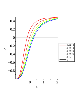
Figure 1: Evolution of the deceleration parameter as a function of redshift

5. Let us now move on to the analysis of the relations connecting the deceleration parameter $q$and the model parameter $\Delta$. For a flat FLRW Universe filled with nonrelativistic matter and BEDE with relative densities $\Omega_{m}$ and $\Omega_{e}$ the deceleration parameter is equal to [30, 31]

$$q=-\frac{\dot{H}}{H^{2}}-1=\frac{\left(\Delta+1\right)\Omega_{m}-\Delta}{\Delta-\left(\Delta-2\right)\Omega_{m}}$$ (19)

where

$$\begin{array}[]{l}{\Omega_{m}=\frac{\Omega_{m0}\left(1+z\right)^{3}}{\frac{\Omega_{m0}\left(1+z\right)^{3}+\Omega_{e0}}{}},}\\ {\Omega_{e}=\frac{\Omega_{e0}}{\frac{\Omega_{m0}\left(1+z\right)^{3}+\Omega_{e0}}{}},}\\ {\Omega_{m}+\Omega_{e}=1}\end{array}$$ (20)

For a Universe of arbitrary curvature [31]

$$q=\frac{\left(\Delta+1\right)\Omega_{m}-\Delta\left(\Omega_{k}+1\right)}{\Delta+\left(\Delta-2\right)\Omega_{k}-\left(\Delta-2\right)\Omega_{m}},$$ (21)

where $\Omega_{k}=\frac{k}{a^{2}H^{2}}$.

Expression (19) for the deceleration parameter has the correct asymptotics, independent of $\Delta$. In the early Universe $\Omega_{m}=1(z\to\infty)\;q=\frac{1}{2}$, and in the distant future $\Omega_{m}=0\left(z=-1\right)\quad q=-1$.

The evolution of the deceleration parameter $q$ as a function of redshift$z$, described by expression (19) is shown in Fig. 1

Fig.1 shows that the BEDE model can well explain the history of the Universe, including the era of matter dominance.

As we noted above, this approach represents a “blind” search of parameters in order to find the optimal value of the parameter$\Delta$. The optimality criterion can, for example, be the prediction of a fairly well-known value of redshift$\left(z_{q=0}\right)$, at which the transition from deceleration to accelerated expansion occurs, i.e. the deceleration parameter changes sign [31, 32, 33, 34, 35, 36, 37]. From (19) we find

$$q=0\to\Delta=\frac{\Omega_{m}\left(z_{q=0}\right)}{1-\Omega_{m}\left(z_{q=0}\right)}$$ (22)

From (22) follows that

$$z_{q=0}=\left(\frac{\Delta\Omega_{e0}}{\Omega_{m0}}\right)^{1/3}-1$$ (23)

For the value of the parameter $\Delta=2$ (in this case, the density BEDE is independent of time), expression (22) reproduces the transition acceleration in the SCM

The maximum transition redshift in the BEDE model is achieved at a degree of fractality $\Delta=1$ and equal to$z_{q=0}^{\max}\simeq{\rm 0.286}$. Coordination of the values of transition acceleration in the BEDE model with the corresponding value in the SCM requires going beyond the permissible values of the fractality parameter$0\leq\Delta\leq 1$.

6.Thus, we see that although the BEDE model generally correctly describes the evolution of the FLRW Universe, it leads to a too late transition from deceleration to accelerated expansion $\left(z_{q=0}^{BEDE}<z_{q=0}^{SCM}\right)$. One possibility to resolve this contradiction is to include interaction between dark matter and BEDE [38, 39]. The cosmographic approach to determining the parameters of models involving such interactions will be the subject of further research.

References

- [1] Yuriy L. Bolotin, V.A. Cherkaskiy, O. Yu. Ivashtenko, M. I. Konchatnyi, and L. G. Zazunov. Applied cosmography: A pedagogical review, 2018.
- [2] Matt Visser. Cosmography: Cosmology without the einstein equations. General Relativity and Gravitation, 37(9):1541–1548, September 2005.
- [3] Matt Visser. Jerk, snap and the cosmological equation of state. Classical and Quantum Gravity, 21(11):2603–2615, April 2004.
- [4] Steven Weinberg. Gravitation and Cosmology: Principles and Applications of the General Theory of Relativity. John Wiley and Sons, New York, 1972.
- [5] Allan R. Sandage. Cosmology: a search for two numbers. Physics Today, 23(2):34–41, January 1970.
- [6] Yuriy L. Bolotin, Danylo A. Erokhin, and Oleg A. Lemets. Expanding universe: slowdown or speedup? Uspekhi Fizicheskih Nauk, 182(9):941–986, 2012.
- [7] Peter K. S. Dunsby and Orlando Luongo. On the theory and applications of modern cosmography. International Journal of Geometric Methods in Modern Physics, 13(03):1630002, March 2016.
- [8] John D. Barrow. The area of a rough black hole. Physics Letters B, 808:135643, September 2020.
- [9] Jacob D. Bekenstein. Black holes and the second law. Lett. Nuovo Cim., 4:737–740, 1972.
- [10] Jacob D. Bekenstein. Black holes and entropy. Phys. Rev. D, 7:2333–2346, Apr 1973.
- [11] Shuang Wang, Yi Wang, and Miao Li. Holographic dark energy. Physics Reports, 696:1–57, June 2017.
- [12] Miao Li. A model of holographic dark energy. Physics Letters B, 603(1):1–5, 2004.
- [13] Emmanuel N. Saridakis. Restoring holographic dark energy in brane cosmology. Physics Letters B, 660(3):138–143, February 2008.
- [14] Emmanuel N. Saridakis. Barrow holographic dark energy. Physical Review D, 102(12), December 2020.
- [15] Fotios K. Anagnostopoulos, Spyros Basilakos, and Emmanuel N. Saridakis. Observational constraints on barrow holographic dark energy, 2020.
- [16] Shikha Srivastava and Umesh Kumar Sharma. Barrow holographic dark energy with hubble horizon as ir cutoff. International Journal of Geometric Methods in Modern Physics, 18(01):2150014, November 2020.
- [17] Emmanuel N. Saridakis. Modified cosmology through spacetime thermodynamics and barrow horizon entropy. Journal of Cosmology and Astroparticle Physics, 2020(07):031–031, July 2020.
- [18] Maciej Dunajski and Gary Gibbons. Cosmic jerk, snap and beyond. Classical and Quantum Gravity, 25(23):235012, November 2008.
- [19] Yuri L. Bolotin, Alexander Kostenko, Oleg A. Lemets, and Danylo A. Yerokhin. Cosmological evolution with interaction between dark energy and dark matter. International Journal of Modern Physics D, 24(03):1530007, 2015.
- [20] Purba Mukherjee and Narayan Banerjee. Revisiting a non-parametric reconstruction of the deceleration parameter from combined background and the growth rate data. Physics of the Dark Universe, 36:100998, June 2022.
- [21] Abdulla Al Mamon and Kazuharu Bamba. Observational constraints on the jerk parameter with the data of the hubble parameter, 2018.
- [22] Zhong-Xu Zhai, Ming-Jian Zhang, Zhi-Song Zhang, Xian-Ming Liu, and Tong-Jie Zhang. Reconstruction and constraining of the jerk parameter from ohd and sne ia observations. Physics Letters B, 727(1–3):8–20, November 2013.
- [23] Hsin-Yu Chen, Jose María Ezquiaga, and Ish Gupta. Cosmography with next-generation gravitational wave detectors, 2024.
- [24] Salvatore Capozziello and Rocco D’Agostino. Reconstructing the distortion function of non-local cosmology: a model-independent approach, 2023.
- [25] Nobuyoshi Komatsu and Shigeo Kimura. General form of entropy on the horizon of the universe in entropic cosmology. Physical Review D, 93(4), February 2016.
- [26] Nobuyoshi Komatsu and Shigeo Kimura. Entropic cosmology in a dissipative universe. Phys. Rev. D, 90:123516, Dec 2014.
- [27] Spyros Basilakos, Andreas Lymperis, Maria Petronikolou, and Emmanuel N. Saridakis. Barrow holographic dark energy with varying exponent, 2023.
- [28] Shin’ichi Nojiri, Sergei D. Odintsov, and Emmanuel N. Saridakis. Modified cosmology from extended entropy with varying exponent. The European Physical Journal C, 79(3), March 2019.
- [29] Shin’ichi Nojiri, Sergei D. Odintsov, and Tanmoy Paul. Barrow entropic dark energy: A member of generalized holographic dark energy family. Physics Letters B, 825:136844, February 2022.
- [30] Anirudh Pradhan, Archana Dixit, and Vinod Kumar Bhardwaj. Barrow hde model for statefinder diagnostic in flrw universe. International Journal of Modern Physics A, 36(04):2150030, February 2021.
- [31] Archana Dixit, Vinod Kumar Bharadwaj, and Anirudh Pradhan. Barrow hde model for statefinder diagnostic in non-flat frw universe, 2021.
- [32] Omer Farooq and Bharat Ratra. Hubble parameter measurement constraints on the cosmological deceleration-acceleration transition redshift. The Astrophysical Journal, 766(1):L7, March 2013.
- [33] Omer Farooq, Foram Ranjeet Madiyar, Sara Crandall, and Bharat Ratra. Hubble parameter measurement constraints on the redshift of the deceleration–acceleration transition, dynamical dark energy, and space curvature. The Astrophysical Journal, 835(1):26, January 2017.
- [34] Abdulla Al Mamon. Constraints on a generalized deceleration parameter from cosmic chronometers. Modern Physics Letters A, 33(10n11):1850056, April 2018.
- [35] Abdulla Al Mamon and Kazuharu Bamba. Observational constraints on the jerk parameter with the data of the hubble parameter, 2018.
- [36] Abdulla Al Mamon and Sudipta Das. A parametric reconstruction of the deceleration parameter. The European Physical Journal C, 77, 10 2016.
- [37] Juan Magaña, Víctor H. Cárdenas, and Verónica Motta. Cosmic slowing down of acceleration for several dark energy parametrizations. Journal of Cosmology and Astroparticle Physics, 2014(10):017–017, October 2014.
- [38] Abdulla Al Mamon, Andronikos Paliathanasis, and Subhajit Saha. Dynamics of an interacting barrow holographic dark energy model and its thermodynamic implications. The European Physical Journal Plus, 136(1), January 2021.
- [39] Giuseppe Gaetano Luciano and Jaume Giné. Generalized interacting barrow holographic dark energy: cosmological predictions and thermodynamic considerations, 2022.