Gluon generalized parton distributions of the proton at non-zero skewness

Abstract

Using a recently developed light-front spectator model that incorporates gluon, where the light-front wave functions are modeled from the soft-wall AdS/QCD prediction, we examine the leading twist gluon generalized parton distributions (GPDs) inside the proton. We derive the chirally even and odd distributions by using the overlap representation of the light-front wave functions. In terms of GPDs at non-zero skewness, we investigate the entire three-dimensional representation of gluons. We analyse the gluon impact parameter distributions at $\xi=0$ using the Fourier transform of GPDs. We address the total angular momentum contribution of the gluons by using the Ji’s sum rule and also give our predictions for both the canonical and kinetic orbital angular momentum in the light-cone gauge.

I Introduction

One of the most difficult tasks in hadronic physics is to understand the three-dimensional structure of nucleons in terms of its constituent quarks and gluons, although parton distribution functions (PDFs) describe the distributions of the longitudinal momentum and polarization carried by quarks and gluons in a fast-moving hadron. The PDFs are the diagonal, or forward matrix elements of particular operators, providing a probability interpretation in terms of distributions and examining space-time correlations along the light-cone more extensively. It is only possible to fully understand the correlations by taking into account the non-diagonal, or off-forward matrix elements of the same operators. These non-diagonal matrix elements can be parametrized in terms of generalized parton distributions (GPDs) Müller et al. (1994); Diehl (2003); Belitsky and Radyushkin (2005); Goeke et al. (2001); Boffi and Pasquini (2007); Brodsky et al. (2006). The GPDs encode spatial as well as partonic spin structure in a nucleon. The GPDs can be related to the generalized transverse momentum distributions (GTMDs) Meissner et al. (2009); Lorcé and Pasquini (2013); Kanazawa et al. (2014); Mukherjee et al. (2014); Hagiwara et al. (2016); Ojha et al. (2023); Maji et al. (2022); Mukherjee et al. (2015); More et al. (2018); Chakrabarti et al. (2020a); Maji et al. (2017); Zhang et al. (2023). In the forward limit, or when the momentum transfer is zero, they reduce to PDFs, that are accessible through inclusive processes. The second moment of the GPDs is related to the gravitational form factors (GFFs), which are the form factors of the energy-momentum tensor Ji (1997a); Radyushkin (1997); Ji and Osborne (1998); Ji (1998); Blumlein et al. (1999); Goeke et al. (2001); Guo et al. (2023a); Hackett et al. (2023); Garcia Martin-Caro et al. (2023); Burkert et al. (2023a); More et al. (2023); Choudhary et al. (2022); de Téramond et al. (2021). The GPDs or the GFFs are experimentally accessed through exclusive processes such as deeply virtual Compton scattering (DVCS) or deeply virtual vector-meson productions (DVMP). The GFFs, and therefore, the GPDs, contain important information about the mass, angular momentum and mechanical properties of the nucleon Polyakov and Schweitzer (2018); Lorcé et al. (2019); Chakrabarti et al. (2020b); Mondal (2017); Li and Vary (2023); Burkert et al. (2023b); Choudhary et al. (2022); Singh et al. (2023); More et al. (2023, 2022). The GPDs are described as functions of three variables: longitudinal momentum fraction $x$ of the parton, longitudinal momentum fraction transferred in the process which is given by skewness $\xi$ and square of the total momentum transferred $t=\Delta^{2}$. In addition to providing information on the longitudinal behavior in momentum space along the direction in which the nucleon is moving, the GPDs also provide insights into how partons are spatially distributed in the transverse plane, making them an effective tool for studying hadron structure in three dimensions Burkardt (2003, 2006). Experimentally, determining GPDs in unique processes is quite difficult and demands high luminosity and resolution. First focused studies were therefore designed and carried out in the last decade Adloff et al. (2000); Airapetian et al. (2001). Through the production of vector mesons, they are experimentally accessible. Data from experiments like H1, ZEUS, HERMES Adloff et al. (2001); Aktas et al. (2005); Aaron et al. (2009); Chekanov et al. (2003); Airapetian et al. (2010); Airapetian et al. (2012a, b) have played a major role in the effort to extract the GPDs, also these will be explored in the JLab 12 GeV upgrade as well as the upcoming electron-ion collider (EIC) Abdul Khalek et al. (2022). The Fourier transform of GPDs with respect to the transverse momentum transfer, $\Delta_{\perp}$, gives the impact parameter dependent parton distributions, also known as IPDs, which tell us how the partons of a given longitudinal momentum are distributed in transverse position space Burkardt (2003, 2006). Impact parameter measures the transverse separation of an active parton from the system’s center of momentum. The spin densities can be represented in terms of impact parameter dependent GPDs for different proton polarizations Lin et al. (2023); Maji et al. (2017); Guo et al. (2022); Mukherjee et al. (2015); Mondal and Chakrabarti (2015). A more general description of the nucleon is given in terms of the GTMDs Lorce and Pasquini (2011); Lorce et al. (2012), that help to access spin-spin and spin-orbit correlation of the gluon Bhattacharya et al. (2022). The GTMDs are called mother distributions as the TMDs can be extracted from the GTMDs in the forward limit $\Delta_{\perp}=0$, and the GPDs can be obtained in impact parameter space upon integration over ${\bf p}_{\perp}$. The two-dimensional Fourier transform of GTMDs yields Wigner distributions Ji (2003); Belitsky et al. (2004), which characterize the five-dimensional phase-space distribution of partons within the nucleon. These distributions play a crucial role in revealing spin-orbital correlations, essential for extracting parton orbital angular momentum Ji et al. (2012); Mukherjee et al. (2015); Hatta (2012); More et al. (2018).

Although it is known that gluon contributes significantly to the proton spin, the gluon distributions and contribution to the spin Jaffe (1996) and OAM are less explored as compared to the quarks. This is because, in most phenomenological models of the proton, there is no gluon. Only very recently, studies have been started in this direction Adare et al. (2009); Boer et al. (2011); Bhattacharya et al. (2023a, b); Gurjar et al. (2022); Xu et al. (2022); Chakrabarti et al. (2023); Zhou et al. (2022); Abdallah et al. (2022); Ji et al. (2021); Yang et al. (2017); Sato et al. (2016); de Florian et al. (2014). In this work, we use a recently developed spectator model Chakrabarti et al. (2023) that incorporates the active gluon, to investigate the gluon GPDs at nonzero skewness ($\xi\neq 0$) in the proton. There are eight gluon GPDs for the proton at leading-twist. Four of them ($H^{g}$, $E^{g}$, $\tilde{H}^{g}$, and $\tilde{E}^{g}$) are chirally even and other four GPDs ($H_{T}^{g}$, $E_{T}^{g}$ $\tilde{H}_{T}^{g}$, and $\tilde{E}_{T}^{g}$) are chirally odd. The GPDs $H^{g}$ and $\tilde{H}^{g}$ are related to the unpolarized and polarized gluon PDFs, respectively. In the impact parameter space, they provide the spin densities of the unpolarized and circularly polarized gluons in a longitudinally polarized proton. The GPD $E^{g}$ is related to the distortion of the unpolarized gluon distribution in a transversely polarized proton, in some models, this GPD is related to the gluon Sivers function which is a T-odd TMDPDF Meissner et al. (2007). Chiral odd GPDs are also accessible in specific processes like deeply virtual Compton scattering or deeply virtual meson generation. They are more difficult to probe experimentally than chiral even GPDs, as they need another chiral-odd object in the amplitude to combine.

As stated above, the GTMDs as well as the GPDs are important to understand the angular momentum contribution of the gluons to the nucleon spin, and its orbital angular momentum (OAM). The decomposition of the total angular momentum of the nucleon into spin and OAM is not unique Leader and Lorcé (2014). There are two well-known decompositions, known as the kinetic and canonical decompositions, available in the literature Wakamatsu (2010); Ji (1997b); Leader and Lorcé (2014). We also present a calculation of the gluon contribution to the total angular momentum of the proton as well as the OAM in different decompositions in our model.

The work is arranged in the following manner: In section II, we briefly review the light front gluon spectator model. In section III, we discuss the general definition of gluon GPD correlator which allows us to assess both chiral-even and chiral-odd GPDs at leading twist with both zero and non-zero skewness. In section IV we evaluate the chiral-even gluon GTMDs and we present a discussion on gluon orbital angular momentum and spin-correlation distributions. In section V we present the impact parameter dependent generalized parton distributions at zero skewness. Finally, in Section VI we present our conclusions and outlook. Many supplementary formulae explaining the details of the parametrization are presented in the Appendix.

II light front wave function

To investigate the gluon distribution functions within the proton, we have recently formulated a light-front spectator model for the proton in which gluon is considered as an active parton. A detailed description about the model construction can be found in Ref. Chakrabarti et al. (2023). Apart from the struck gluon, the remaining components, including the three valence quarks and any additional gluons or sea quarks, collectively form the spectator system. We consider the proton as a composite system of spin-1 gluon and spin-1/2 spectator.

The model is based on the light-cone approach with $x^{\pm}=x^{0}\pm x^{3}$. We choose a reference frame where the transverse momentum of the proton vanishes, i.e., $P=(P^{+},\frac{M^{2}}{P^{+}},\textbf{0}_{\perp})$. The momentum of active parton is given by $p=(xP^{+},\frac{p^{2}+\textbf{p}_{\perp}^{2}}{xP^{+}},\textbf{p}_{\perp})$ and the momentum of the spectator $P_{X}=((1-x)P^{+},P^{-}_{X},-\textbf{p}_{\perp})$. The variable $x=p^{+}/P^{+}$ represents the fraction of longitudinal momentum carried by the struck gluon. Therefore, the proton state can be written as a two-particle Fock-state expansion with proton helicity $J_{z}=\pm\frac{1}{2}$ as Brodsky et al. (2001),

$$|P;\uparrow(\downarrow)\rangle=\int\frac{\mathrm{d}^{2}{\bf p}_{\perp}\mathrm{d}x}{16\pi^{3}\sqrt{x(1-x)}}\times\Bigg{[}\psi_{+1+\frac{1}{2}}^{\uparrow(\downarrow)}\left(x,{\bf p}_{\perp}\right)\left|+1,+\frac{1}{2};xP^{+},{\bf p}_{\perp}\right\rangle+\psi_{+1-\frac{1}{2}}^{\uparrow(\downarrow)}\left(x,{\bf p}_{\perp}\right)\left|+1,-\frac{1}{2};xP^{+},{\bf p}_{\perp}\right\rangle$$

$$+\psi_{-1+\frac{1}{2}}^{\uparrow(\downarrow)}\left(x,{\bf p}_{\perp}\right)\left|-1,+\frac{1}{2};xP^{+},{\bf p}_{\perp}\right\rangle+\psi_{-1-\frac{1}{2}}^{\uparrow(\downarrow)}\left(x,{\bf p}_{\perp}\right)\left|-1,-\frac{1}{2};xP^{+},{\bf p}_{\perp}\right\rangle\bigg{]},$$ (1)

where $\psi_{\lambda_{g}\lambda_{X}}^{\uparrow(\downarrow)}(x,{\bf p}_{\perp})$ are the two-particle LFWFs, which represents the probability amplitudes to find constituents corresponding to the two-particle Fock state $|\lambda_{g},\lambda_{X};xP^{+},{\bf p}_{\perp}\rangle$ with longitudinal momentum $xP^{+}$, transverse momentum ${\bf p}_{\perp}$ and helicities $\lambda_{g}$ and $\lambda_{X}$ in the proton. Here $\lambda_{g}$ and $\lambda_{X}$ stand for the helicity components of the active gluon and spectator, respectively.

The two-particle LFWFs of the proton with $J_{z}=+1/2$ have the following form  Chakrabarti et al. (2023),

$$\psi_{+1+\frac{1}{2}}^{\uparrow}\left(x,{\bf p}_{\perp}\right) = -\sqrt{2}\frac{(-p^{1}_{\perp}+ip^{2}_{\perp})}{x(1-x)}\varphi(x,{\bf p}_{\perp}^{2}),$$

$$\psi_{+1-\frac{1}{2}}^{\uparrow}\left(x,{\bf p}_{\perp}\right) = -\sqrt{2}\bigg{(}M-\frac{M_{X}}{(1-x)}\bigg{)}\varphi(x,{\bf p}_{\perp}^{2}),$$

$$\psi_{-1+\frac{1}{2}}^{\uparrow}\left(x,{\bf p}_{\perp}\right) = -\sqrt{2}\frac{(p^{1}_{\perp}+ip^{2}_{\perp})}{x}\varphi(x,{\bf p}_{\perp}^{2}),$$

$$\psi_{-1-\frac{1}{2}}^{\uparrow}\left(x,{\bf p}_{\perp}\right) = 0,$$ (2)

where both $M$ and $M_{X}$ represent the masses of the proton and spectator. Similarly, the two-particle LFWFs of a proton with $J_{z}=-1/2$ have the form,

$$\psi_{+1+\frac{1}{2}}^{\downarrow}\left(x,{\bf p}_{\perp}\right) = 0,$$

$$\psi_{+1-\frac{1}{2}}^{\downarrow}\left(x,{\bf p}_{\perp}\right) = -\sqrt{2}\frac{(-p^{1}_{\perp}+ip^{2}_{\perp})}{x}\varphi(x,{\bf p}_{\perp}^{2}),$$

$$\psi_{-1+\frac{1}{2}}^{\downarrow}\left(x,{\bf p}_{\perp}\right) = -\sqrt{2}\bigg{(}M-\frac{M_{X}}{(1-x)}\bigg{)}\varphi(x,{\bf p}_{\perp}^{2}),$$

$$\psi_{-1-\frac{1}{2}}^{\downarrow}\left(x,{\bf p}_{\perp}\right) = -\sqrt{2}\frac{(p^{1}_{\perp}+ip^{2}_{\perp})}{x(1-x)}\varphi(x,{\bf p}_{\perp}^{2}).$$ (3)

Where $\varphi(x,{\bf p}_{\perp}^{2})$ is the modified form of the soft-wall AdS/QCD wave function, which is modeled by introducing the parameters $a$ and $b$. The expression for the wave function $\varphi(x,{\bf p}_{\perp}^{2})$ is modified by $x$ and $1-x$ factors, which explains the small and large $x$ region behaviour of the PDFs. The complete form of the modified soft-wall AdS/QCD wave function is given as Gutsche et al. (2014); Chakrabarti et al. (2023),

$$\varphi(x,{\bf p}_{\perp}^{2})=N_{g}\frac{4\pi}{\kappa}\sqrt{\frac{\log[1/(1-x)]}{x}}x^{b}(1-x)^{a}\exp{\bigg{[}-\frac{\log[1/(1-x)]}{2\kappa^{2}x^{2}}{\bf p}_{\perp}^{2}\bigg{]}}$$ (4)

where $\kappa$ is the AdS scale parameter which is given as $\kappa=0.4$ GeV Brodsky et al. (2015). While, $a,~{}b$, and $N_{g}$ are the model parameters which are fixed by fitting the NNPDF3.0 NLO gluon unpolarized PDF data set at initial scale $\mu_{0}=2$ GeV and can be found in Ref. Chakrabarti et al. (2023). For the stability of the proton, the sum of constituent masses is considered higher than the proton mass, i.e., $M_{X}>M$ Bacchetta et al. (2020).

III Gluon GPDs

In the light-cone gauge $A^{+}=0$, the off-forward matrix elements of the bilocal currents of light-front correlation functions define the four leading twist gluon helicity conserving GPDs Diehl (2001, 2003); Ji (1998)

$$\frac{1}{P^{+}}\int\frac{dz^{-}}{2\pi}\,e^{ixP^{+}z^{-}}\langle p^{\prime},\lambda^{\prime}|\,F^{+i}(-{\textstyle\frac{z}{2}})\,F^{+i}({\textstyle\frac{z}{2}})\,\,|p,\lambda\rangle\Big{|}_{\begin{subarray}{c}z^{+}=0\\ \mathbf{z}_{T}=0\end{subarray}}=\frac{1}{2P^{+}}\bar{u}(p^{\prime},\lambda^{\prime})\left[H^{g}\,\gamma^{+}+E^{g}\,\frac{i\sigma^{+\alpha}\Delta_{\alpha}}{2M}\right]u(p,\lambda),$$ (5)

$$-\frac{i}{P^{+}}\int\frac{dz^{-}}{2\pi}\,e^{ixP^{+}z^{-}}\langle p^{\prime},\lambda^{\prime}|\,F^{+i}(-{\textstyle\frac{z}{2}})\,\tilde{F}^{+i}({\textstyle\frac{z}{2}})\,\,|p,\lambda\rangle\Big{|}_{\begin{subarray}{c}z^{+}=0\\ \mathbf{z}_{T}=0\end{subarray}}=\frac{1}{2P^{+}}\bar{u}(p^{\prime},\lambda^{\prime})\left[\tilde{H}^{g}\,\gamma^{+}\gamma_{5}+\tilde{E}^{g}\,\frac{\gamma_{5}\Delta^{+}}{2M}\,\,\right]u(p,\lambda),$$ (6)

where $\tilde{F}^{\alpha\beta}=\frac{1}{2}\epsilon^{\alpha\beta\gamma\delta}F_{\gamma\delta}$ is the dual field strength tensor and a summation over $i=1,2$ is implied. Similarly, the remaining four gluon helicity flip GPDs involves the matrix elements of gluon tensor operator $\mathbf{S}F^{+i}(-z/2)F^{+j}(z/2)$, where S represents the symmetrization operator in $i$ and $j$ and can be given as,

$$-\frac{1}{P^{+}}\int\frac{dz^{-}}{2\pi}\,e^{ixP^{+}z^{-}} \langle p^{\prime},\lambda^{\prime}|\,{\mathbf{S}}F^{+i}(-{\textstyle\frac{z}{2}})\,F^{+j}({\textstyle\frac{z}{2}})\,|p,\lambda\rangle\Big{|}_{\begin{subarray}{c}z^{+}=0\\ \mathbf{z}_{T}=0\end{subarray}}={\mathbf{S}}\,\frac{1}{2P^{+}}\,\frac{P^{+}\Delta^{j}-\Delta^{+}P^{j}}{2MP^{+}}$$

$$\times\bar{u}(p^{\prime},\lambda^{\prime})\Bigg{[}H_{T}^{g}\,i\sigma^{+i}+\tilde{H}_{T}^{g}\,\frac{P^{+}\Delta^{i}-\Delta^{+}P^{i}}{M^{2}}+E_{T}^{g}\,\frac{\gamma^{+}\Delta^{i}-\Delta^{+}\gamma^{i}}{2M}+\tilde{E}_{T}^{g}\,\frac{\gamma^{+}P^{i}-P^{+}\gamma^{i}}{M}\,\Bigg{]}u(p,\lambda),\hskip 20.00003pt$$ (7)

where $u$ $\left(\bar{u}\right)$ are the light-front spinors with $p$ $(p^{\prime})$ and $\lambda$ $(\lambda^{\prime})$ the momenta and the helicity of the initial (final) state of proton, respectively. In the symmetric frame, the kinematic variables are denoted as: the average momentum $P^{\mu}=\frac{(p+p^{\prime})^{\mu}}{2}$, momentum transfer $\Delta^{\mu}=p^{\prime\mu}-p^{\mu}$, the skewness $\xi=-\Delta^{+}/2P^{+}$, and the invariant momentum transfer in the process $t=\Delta^{2}$. The standard form of the gluon field strength tensor $F_{a}^{\mu\nu}(x)$ is given in terms of structure constant $f_{abc}$ as follows

$$F^{\mu\nu}_{a}(x)=\partial^{\mu}A^{\nu}_{a}(x)-\partial^{\nu}A_{a}^{\mu}(x)+gf_{abc}A_{b}^{\mu}(x)A_{c}^{\nu}(x).$$ (8)

We choose light cone gauge $A^{+}=0$, which fixes the gauge link between the fields to be unity. It also implies that $F^{+i}=\partial^{+}A^{i}$ which simplifies the calculation. The operator $F^{+i}(-\frac{z}{2})$ is associated with incoming gluon while $F^{+j}(\frac{z}{2})$ is associated with an outgoing gluon. We use the light-cone quantization framework to obtain the gluon distributions in terms of light-cone helicity amplitudes. We then define the following helicity amplitudes which are connected to different gluon GPDs based on the different proton and gluon helicity configurations Diehl (2003, 2001); Boffi and Pasquini (2007); Maji et al. (2017):

$$A_{\lambda^{\prime}\mu^{\prime},\lambda\mu}=\frac{1}{P^{+}}\int\frac{dz^{-}}{2\pi}\,e^{ixP^{+}z^{-}}\langle p^{\prime},\lambda^{\prime}|\,\epsilon^{i}(\mu^{\prime})F^{+i}(-{\textstyle\frac{z}{2}})\,F^{+j}({\textstyle\frac{z}{2}})\epsilon^{*j}(\mu)\,|p,\lambda\rangle\Big{|}_{z^{+}=0,\,\mathbf{z}_{T}=0}\,$$ (9)

where $\mu$ $(\mu^{\prime})$ denotes the the gluon helicity of the initial (final) state and $\epsilon$ is the two-dimensional gluon polarization vectors. Parity invariance results following relation among the various helicity amplitudes as,

$$A_{-\lambda^{\prime}-\mu^{\prime},-\lambda-\mu}=(-1)^{\lambda^{\prime}-\mu^{\prime}-\lambda+\mu}\,(A_{\lambda^{\prime}\mu^{\prime},\lambda\mu})^{\ast}$$ (10)

III.1 GPDs at non zero skewness

The internal structure of the proton has primarily been investigated within the confines of the $\xi=0$ limit in most studies. However, in order to fully uncover the wealth of information available within the three-dimensional momentum transfer space, it is imperative to assess the GPDs at non-zero skewness values. Recent theoretical works Guo et al. (2023b, c) have started to explore GPDs at non-zero skewness. In fact, skewness is typically non-zero in experiments. The GPDs evolve with the scale differently in different kinematical regions Diehl et al. (2001): for the quark GPDs, (i) $x\geq\xi$ corresponds to the situation when an active quark of initial longitudinal momentum fraction of $x+\xi$ struck with a photon and come back to the nucleon with longitudinal momentum fraction $x-\xi$; (ii) $x\leq-\xi$ corresponds the distributions of anti-quarks where both the longitudinal momentum fractions $x+\xi$ and $x-\xi$ are negative; both the $x\geq\xi$ and $x\leq-\xi$ regions are known as Dokshitzer-Gribov-Lipatov-Altarelli-Parisi (DGLAP) domain; (iii) in the third region $-\xi\leq x\leq\xi$, which is known as Efremov-Radyushkin-Brodsky-Lepage (ERBL) region the GPDs correspond to the process in which a quark of longitudinal momentum $x+\xi$ interact with a virtual photon and emit an anti-quark of longitudinal momentum $\xi-x$. Here, we investigate the gluon GPDS, in which the active parton is a gluon, in the DGLAP region ($x>\xi$ only), as in the ERBL region, the GPDs would involve particle number changing overlaps involving higher Fock components of the LFWFs, which is beyond the scope of the present work. The helicity amplitudes, $A_{\lambda^{\prime}\mu^{\prime},\lambda\mu}$ include specific information regarding the initial and final helicities of the proton and gluon. The chiral-even GPDs are defined in terms of helicity amplitudes wherein the helicity of the gluon does not change and the helicity of the nucleon does. While in the chiral odd GPDs, gluon flips its helicity.

In the reference frame where the momenta $\vec{p}$ and $\vec{p}^{\prime}$ lie in the $x-z$ plane, the chiral-even GPDs can be expressed through the gluon helicity conserving amplitudes within the helicity basis as follows Diehl (2001); Maji et al. (2017); Boffi and Pasquini (2007) :

$$H^{g} = \frac{1}{\sqrt{1-\xi^{2}}}T^{g}_{1}-\frac{2M\xi^{2}}{\sqrt{t_{0}-t}(1-\xi^{2})}T^{g}_{3},$$ (11)

$$E^{g} = -\frac{2M}{\epsilon\sqrt{t_{0}-t}}T^{g}_{3},$$ (12)

$$\widetilde{H}^{g} = \frac{1}{\sqrt{1-\xi^{2}}}T^{g}_{2}+\frac{2M\xi}{\sqrt{t_{0}-t}(1-\xi^{2})}T^{g}_{4},$$ (13)

$$\widetilde{E}^{g} = \frac{2M}{\epsilon\xi\sqrt{t_{0}-t}}T^{g}_{4},$$ (14)

while, the chiral-odd GPDs can be written in terms of gluon helicity non-conserving amplitudes as,

$$H_{T}^{g} = \frac{2M}{\epsilon\sqrt{t_{0}-t}(1-\xi^{2})}\widetilde{T}^{g}_{1}-\frac{4M^{2}\xi}{(t_{0}-t)(1-\xi^{2})\sqrt{1-\xi^{2}}}\widetilde{T}^{g}_{3},$$ (15)

$$E_{T}^{g} = \frac{4M^{2}}{(t_{0}-t)(1-\xi^{2})\sqrt{1-\xi^{2}}}\left(\xi\widetilde{T}^{g}_{3}+\widetilde{T}^{g}_{4}\right)$$ (16)

$$\tilde{E}_{T}^{g} = \frac{4M^{2}}{(t_{0}-t)(1-\xi^{2})\sqrt{1-\xi^{2}}}\left(\widetilde{T}^{g}_{3}+\xi\widetilde{T}^{g}_{4}\right)$$ (17)

$$\tilde{H}_{T}^{g} = 0$$ (18)

where $T^{g}_{i}$ and $\widetilde{T}^{g}_{i}$ are chiral even and chiral-odd helicity basis which are defined as a combination of helicity amplitudes Kriesten et al. (2022) as:

$$T^{g}_{1}=A_{++,++}+A_{-+,-+}, T^{g}_{2}=A_{++,++}-A_{-+,-+},$$

$$T^{g}_{3}=A_{++,-+}+A_{+-,--}. T^{g}_{4}=A_{++,-+}-A_{+-,--},$$ (19)

and

$$\widetilde{T}^{g}_{1}=A_{++,--}+A_{-+,+-}, \widetilde{T}^{g}_{2}=A_{++,--}-A_{-+,+-},$$

$$\widetilde{T}^{g}_{3}=A_{++,+-}+A_{+-,++}, \widetilde{T}^{g}_{4}=A_{++,+-}-A_{+-,++}$$ (20)

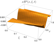
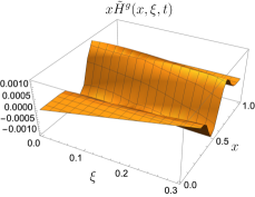
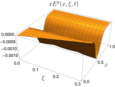
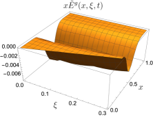
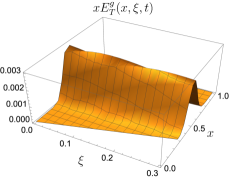
Figure 1: 3D representation of gluon GPDs as a function of gluon longitudinal momentum fraction $x$ and skewness parameter $\xi$ for fixed transverse momentum transfer $-\lvert t\rvert=3$ GeV².

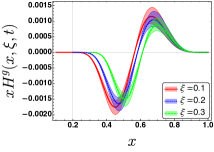
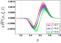
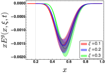
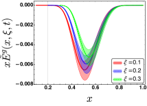
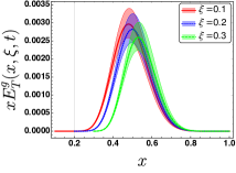
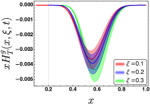
Figure 2: 2D plots of gluon GPDs at $\xi=0.1,0.2$ and $\xi=0.3$ as a function of longitudinal momentum fraction $x$ for a fixed momentum transfer $-\lvert t\rvert=3$ GeV².

Here $t_{0}$ is the minimum value of the transverse momentum transfer $t$, i.e., $t_{0}=-4M^{2}\xi^{2}/(1-\xi^{2})$ for a given value of $\xi$ with $\epsilon=\text{sgn}(D^{i})$ where $D^{i}$ is the $i^{th}$ component of $D^{\alpha}=P^{+}\Delta^{\alpha}-\Delta^{+}P^{\alpha}$ and $t=t_{0}$ for $D^{i}=0$. The matrix elements $T_{i}^{g}$ and $\widetilde{T}_{i}^{g}$ can be written in terms of overlap of light-front wavefunctions. The detailed calculation and expressions for the above matrix elements are given in the Appendix A. Using the equations (54 -61) in the above relations we can get the expressions for individual GPDs at non-zero skewness.

Fig. 1 depicts both the chiral even and chiral-odd GPDs in three-dimensional momentum space, with skewness parameter, $\xi$ and $x$ at a fixed transverse momentum transfer of $-\lvert t\rvert=3$ GeV². Though the GPDs are oscillatory in $x$-space, they vary monotonically with $\xi$. As shown in Fig. 1 the distributions exhibit non-zero values in the $x\geq\xi$ region only. The 3D distribution of $xH^{g}$ shows the behavior of unpolarized GPD. The amplitude of the distribution depends on the value of $x$ and $\xi$ in such a way that it is close to zero when $x$ is very close to $\xi$ but the position of the peak in $x$ depends on the value of $\xi$. A similar kind of behavior is also shown by $x\tilde{H}^{g}$ distribution with a magnitude almost half of the magnitude of the $xH^{g}$ distribution. The forward limit of $H^{g}$ and $\tilde{H}^{g}$ can be related to the unpolarized and helicity PDFs, respectively. Since the results in Fig. 1 are presented at fixed momentum transfer, therefore we cannot relate these results to the forward limit. The distributions $xE^{g}$, $x\tilde{E}^{g}$, and $xH_{T}^{g}$ show similar behavior but of different orders of amplitude.

In Fig. 2, we show the representation of GPDs as a function of the longitudinal momentum fraction variable $x$ within the context of the DGLAP region. These plots are generated at specific values of skewness parameter $\xi$ and momentum transfer $-\lvert t\rvert=3$ GeV². The 2D distributions of $xH^{g}$ and $x\tilde{H}^{g}$ oscillates from negative to positive as they go from small to large $x$ for a particular value of $\xi$ whereas $xE^{g},~{}x\tilde{E}^{g},~{}xE_{T}^{g}$ and $xH_{T}^{g}$ don’t change their signs. The magnitude of both positive and negative peaks depends on the value of $\xi$ as shown in Fig. 2. We observe that the magnitudes of the peaks $xH^{g}$ and $x\tilde{H}^{g}$ decrease and shift towards the large value of $x$ as we increase the value of the skewness parameter. The distributions $x\tilde{E}^{g}$ and $xE_{T}^{g}$ follow a similar trend. While, contrary to these, the magnitudes of $xE^{g}$ and $xH_{T}^{g}$ distributions increase with increasing $\xi$, though the distributions shift towards larger $x$.

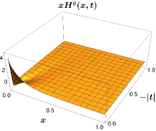
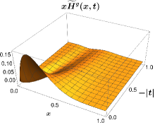
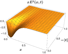
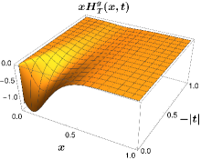
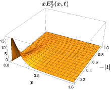
Figure 3: 3D representation of gluon GPDs as a function of gluon longitudinal momentum fraction $x$ and transverse momentum transfer squared $|t|$ (in GeV²) at $\xi=0$.

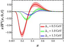
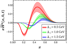
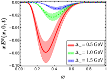
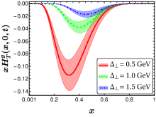
Figure 4: 2D plots of gluon GPDs at $\xi=0$ as a function of longitudinal momentum fraction $x$ at certain values of transverse momentum transfer, $\Delta_{\perp}$ (in GeV).

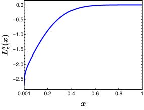
Figure 5: Model predictions on unintegrated gluon kinetic OAM as a function of momentum fraction $x$ .

III.2 GPDs in $\xi=0$ limit

In the limit $\xi\to 0$, the correlation functions of the GPDs reduce to a simplified form, resulting in an expression solely in terms of $x$ and $t=-\Delta_{\perp}^{2}$. In the context of our specific model, we reformulate the equations depicting gluon GPDs at $\xi=0$ limit as

$$H^{g}(x,0,-\Delta_{\perp}^{2})=2N_{g}^{2}x^{2b+1}(1-x)^{2a}\Big{[}\frac{1+(1-x)^{2}}{x^{2}(1-x)^{2}}\left(\frac{\kappa^{2}x^{2}}{\ln\frac{1}{1-x}}-(1-x)^{2}\frac{\Delta_{\perp}^{2}}{4}\right)+\left(M-\frac{M_{X}}{1-x}\right)^{2}\Big{]}exp\left[-\frac{\ln\left(\frac{1}{1-x}\right)(1-x)^{2}}{4\kappa^{2}x^{2}}\Delta_{\perp}^{2}\right]$$ (21)

$$\widetilde{H}^{g}(x,0,-\Delta_{\perp}^{2})=2N_{g}^{2}x^{2b+1}(1-x)^{2a}\Big{[}\frac{1-(1-x)^{2}}{x^{2}(1-x)^{2}}\left(\frac{\kappa^{2}x^{2}}{\ln\frac{1}{1-x}}-(1-x)^{2}\frac{\Delta_{\perp}^{2}}{4}\right)+\left(M-\frac{M_{X}}{1-x}\right)^{2}\Big{]}exp\left[-\frac{\ln\left(\frac{1}{1-x}\right)(1-x)^{2}}{4\kappa^{2}x^{2}}\Delta_{\perp}^{2}\right]$$ (22)

$$E^{g}(x,0,-\Delta_{\perp}^{2})=4MN_{g}^{2}x^{2b}(1-x)^{2a}\left(M(1-x)-M_{X}\right)exp\left[-\frac{\ln\left(\frac{1}{1-x}\right)(1-x)^{2}}{4\kappa^{2}x^{2}}\Delta_{\perp}^{2}\right]$$ (23)

$$H^{g}_{T}(x,0,-\Delta_{\perp}^{2})=4MN_{g}^{2}x^{2b}(1-x)^{2a-1}\left(M(1-x)-M_{X}\right)exp\left[-\frac{\ln\left(\frac{1}{1-x}\right)\Delta_{\perp}^{2}(1-x)^{2}}{4\kappa^{2}x^{2}}\right]$$ (24)

$$E^{g}_{T}(x,0,-\Delta_{\perp}^{2})=4M^{2}N_{g}^{2}x^{2b-1}(1-x)^{2a+1}exp\left[-\frac{\ln\left(\frac{1}{1-x}\right)(1-x)^{2}}{4\kappa^{2}x^{2}}\Delta_{\perp}^{2}\right]$$ (25)

The unpolarized gluon GPD, $H^{g}(x,\xi=0,t)$ given in Eq. (21) reduces to the unpolarized gluon parton distribution function in the forward limit, i.e., $f_{1}^{g}(x)=H^{g}(x,\xi=0,t=0)$. Similarly, the helicity-dependent gluon GPD, $\widetilde{H}^{g}(x,\xi=0,t)$ Eq. (22) gives the gluon helicity pdf in the forward limit as, $g_{1L}^{g}(x)=\widetilde{H}^{g}(x,\xi=0,t=0)$. The gluon helicity GPD provides the gluon spin contribution to the total proton spin $\Delta G=\int{\rm d}xg_{1L}(x)$.

Fig. 3 shows the 3-dimensional behavior of non-zero gluon GPDs of proton in the momentum space at zero skewness with respect to $x$ and $t=-\Delta_{\perp}^{2}$. The unpolarized GPD $H^{g}(x,\xi=0,t)$ at $\xi=0$ shows a sharp peak near $x=0$, only for small $\Delta_{\perp}$. The behaviour around $x\to 0$ drastically changes when $\Delta_{\perp}\geq 0.05$ GeV². It can be better understood from the first plot in Fig. 4. The helicity GPD, $\widetilde{H}^{g}(x,\xi=0,t)$ peaks around $x\approx 0.2$ for smaller values of momentum transfer and its peak decreases a bit slowly as compared to the unpolarized GPD with increasing $x$ and $t$. The helicity GPD $\widetilde{H}^{g}$ also shows a similar trend as the unpolarized GPD, $H^{g}$. A similar kind of behavior of gluon GPDs has been reported in the light-cone spectator model Tan and Lu (2023a). Whereas the unpolarized and helicity GPDs $H^{g}$ and $\widetilde{H}_{g}$ are found to be positive for all values of $x$ and $t$ in basis light-front quantization (BLFQ) Lin et al. (2023) and extended holographic light-front QCD (HLFQCD) Gurjar et al. (2022) approaches. The gluon GPD $E^{g}$, which is also related to the spin-flip gravitational form factor $B(Q^{2})$, is negative in our model. It peaks around $t=0$, which is the forward limit of GPDs, but it does not correspond to any PDF. There are two more non-zero chiral odd gluon GPDs, $H^{g}_{T}$ and $E^{g}_{T}$. We notice that the behaviour of GPD $H^{g}_{T}(x,\xi=0,t)$ is quite similar to the GPD $E^{g}(x,\xi=0,t)$ and they are related to each other as $E^{g}=(1-x)H_{T}^{g}$. Similarly, in Ref. Tan and Lu (2023a); Meissner et al. (2007) the authors have derived a relation between these GPDs as $E^{g}=xH_{T}^{g}$. Both $E^{g}$ and $H_{T}^{g}$ GPDs are negative and peak around the same values of $x$ and $t$. The GPD $E^{g}_{T}(x,\xi=0,t)$ has the largest amplitude in the smaller value of $x$ but it also vanishes with increasing value of $x$. All the GPDs vanish as $x\to 1$, independent of the choice of the momentum transfer.

In Fig. 4 we show the gluon GPDs $H^{g}(x,0,t)$, $\widetilde{H}^{g}$, $E^{g}(x,0,t)$, $H^{g}_{T}(x,0,t)$ and $E^{g}_{T}(x,0,t)$ with $x$ at certain values of momentum transfer $\Delta_{\perp}=0.5,1,1.5$ GeV, respectively.

IV Orbital angular momentum (OAM)

As discussed in the introduction, gluons contribute significantly to the spin of the nucleon. However, the decomposition of the nucleon spin into quark and gluon intrinsic spin and OAM parts is not unique. There is also a question of separation of gluon contribution into those in a gauge invariant manner. Polarised scattering experiments have measured spin asymmetries which are directly sensitive to gluon intrinsic spin. The experimental observables must be related to a gauge-invariant object. This led to a lot of theoretical discussions, a consolidated summary can be found in Leader and Lorcé (2014). There are two main decompositions: kinetic and canonical. Below, we investigate both the kinetic and canonical gluon orbital angular momentum in this model.

IV.1 Kinetic OAM

According to Ji’s sum rule Ji (1997b), the total angular momentum $J^{g}_{z}$ of the gluons can be obtained via the moments of the chiral even helicity conserving GPD $H^{g}$ and helicity non conserving GPD $E^{g}$ through the following sum rule :

$$J^{g}_{z}=\frac{1}{2}\int dxx\left[H^{g}(x,0,0)+E^{g}(x,0,0)\right]$$ (26)

Substituting Equations (21) and (23) into Equation (26), we obtained the gluon’s total angular momentum as $J_{z}^{g}=0.058$ in our model, which aligns with recent findings from the BLFQ collaboration, where $J^{g}_{z}|_{\text{BLFQ}}=0.066$ Lin et al. (2023). However, it should be noted that the scale in Lin et al. (2023) is $0.5$ GeV, which is different from that used in our model.

In an analogous gluon spectator model, with a different wave function, the gluon’s total angular momentum is determined as $J_{z}^{g}=0.19$ Tan and Lu (2023a). The results from this model Tan and Lu (2023a) are consistent with the recent lattice result $J_{z}^{g}=0.187(46)(10)$ obtained by the ETM Collaboration Alexandrou et al. (2020), where the lattice result is provided in the MS scheme at a scale of 2 GeV.

Using the sum rules of gluon GPDs $H^{g},~{}\widetilde{H}^{g}~{}\text{and}~{}E^{g}$ we calculate the gluon OAM in the light-cone gauge from the expression Ji (1997b); Chen et al. (2008); Wakamatsu (2010); Leader and Lorcé (2014)

$$L_{z}^{g}=\int dx\bigg{\{}\frac{1}{2}x\big{[}H^{g}(x,0,0)+E^{g}(x,0,0)\big{]}-\widetilde{H}^{g}(x,0,0)\bigg{\}}$$ (27)

Our numerical results show that $L^{g}_{z}=-0.42$ which means that the gluon kinetic OAM is negative. In Fig. 5 we show the variation of the unintegrated gluonic kinetic OAM with respect to gluon longitudinal momentum fraction $x$. Furthermore, it is noteworthy to highlight that the contribution in the small-$x$ region is not negligible. The kinetic OAM distribution peaks at low $x$, decreasing rapidly as $x$ goes to 1. Similar behavior of gluon kinetic OAM has been reported in another gluon spectator model, with their calculated value for gluon kinetic OAM being $L^{g}_{z}=-0.123$ Tan and Lu (2023a), which is also found to be negative.

IV.2 Canonical OAM from GTMDs

The gluon canonical OAM can be calculated using chirally-even gluon GTMDs in light-cone gauge Jaffe and Manohar (1990); Wakamatsu (2010). In this section, we investigate the gluon GTMDs and canonical OAM in our model.

In order to obtain the gluon GTMDs we used the parametrization Lorcé and Pasquini (2013); Kanazawa et al. (2014); Ji et al. (2013); More et al. (2018) as

$$xW(x,\xi=0,{\bf p}_{\perp},\Delta_{\perp})=\int\frac{dz^{-}}{2\pi}\frac{d^{2}z_{\perp}}{(2\pi)^{2}}e^{ip.z}\bigg{\langle}p+\frac{\Delta_{\perp}}{2}\bigg{|}\Gamma^{ij}F^{+i}\left(-\frac{z}{2}\right)F^{+j}\left(\frac{z}{2}\right)\bigg{|}p-\frac{\Delta_{\perp}}{2}\bigg{\rangle}\Bigg{|}_{z^{+}=0}$$ (28)

where we have suppressed the color indices in the GTMD correlator because we are considering the light-cone gauge in which the gauge link becomes to be unity. The GTMDs, $F_{1,1}$ $F_{1,4}$ describe the distortion of unpolarized partons inside a longitudinally polarized target, whereas $G_{1,1}$ describes how the longitudinally polarized parton distorts their distribution inside an unpolarized target. The light cone overlap representation of the chiral-even gluon GTMDs $F_{1,1}^{g}$, $F_{1,4}^{g}$, $G_{1,1}^{g}$ and $G_{1,4}^{g}$ is given by More et al. (2018); Kanazawa et al. (2014)

$$F_{1,1}^{g}= \frac{1}{2(2\pi)^{3}}\frac{1}{2}\sum_{\Lambda,\mu,\lambda}\epsilon_{\alpha}^{\mu\ast}\epsilon_{\beta}^{\mu}\psi^{\Lambda\ast}_{\mu,\lambda}(x,{\bf p}_{\perp}^{\prime})\psi^{\Lambda}_{\mu,\lambda}(x,{\bf p}_{\perp}^{\prime\prime})$$

$$= \frac{1}{2(2\pi)^{3}}\sum_{\mu,\lambda}(\epsilon_{1}^{\mu\ast}\epsilon_{1}^{\mu}+\epsilon_{2}^{{\mu}\ast}\epsilon_{2}^{\mu})\bigg{[}\psi^{\uparrow\ast}_{\mu,\lambda}(x,{\bf p}_{\perp}^{\prime})\psi^{\uparrow}_{\mu,\lambda}(x,{\bf p}_{\perp}^{\prime\prime})\bigg{]}$$ (29)

$$G_{1,4}^{g}= -\frac{1}{2(2\pi)^{3}}i\epsilon_{T}^{\alpha\beta}\frac{1}{2}\sum_{\Lambda,\mu,\lambda}\epsilon_{\alpha}^{\mu\ast}\epsilon_{\beta}^{\mu}\psi^{\Lambda\ast}_{\mu,\lambda}(x,{\bf p}_{\perp}^{\prime})\psi^{\Lambda}_{\mu,\lambda}(x,{\bf p}_{\perp}^{\prime\prime})$$ (30)

$$= \frac{1}{2(2\pi)^{3}}i\sum_{\mu,\lambda}(\epsilon_{2}^{{\mu}\ast}\epsilon_{1}^{\mu}-\epsilon_{1}^{{\mu}\ast}\epsilon_{2}^{\mu})\bigg{[}\psi^{\uparrow\ast}_{\mu,\lambda}(x,{\bf p}_{\perp}^{\prime})\psi^{\uparrow}_{\mu,\lambda}(x,{\bf p}_{\perp}^{\prime\prime})\bigg{]}$$

$$\tfrac{i(\mathbf{p}_{\perp}\times\boldsymbol{\Delta}_{\perp})_{z}}{M^{2}}\,F_{1,4}^{g} =\frac{1}{2(2\pi)^{3}}\,\frac{1}{2}\sum_{\Lambda,\mu,\lambda}\text{sign}(\Lambda)\left[\psi^{\Lambda\ast}_{\mu,\lambda}(x,{\bf p}_{\perp}^{\prime})\psi^{\Lambda}_{\mu,\lambda}(x,{\bf p}_{\perp}^{\prime\prime})\right]$$

$$=\frac{i}{2(2\pi)^{3}}\sum_{\mu}\textrm{Im}\!\left[\psi^{\uparrow\ast}_{\mu,+\frac{1}{2}}(x,{\bf p}_{\perp}^{\prime})\psi^{\uparrow}_{\mu,+\frac{1}{2}}(x,{\bf p}_{\perp}^{\prime\prime})\right],$$ (31)

$$-\tfrac{i(\mathbf{p}_{\perp}\times\boldsymbol{\Delta}_{\perp})_{z}}{M^{2}}\,G_{1,1}^{g} =\frac{1}{2(2\pi)^{3}}\,\frac{1}{2}\sum_{\Lambda,\lambda,\mu}{\rm sign}(\mu)\left[\psi^{\Lambda\ast}_{\mu,\lambda}(x,{\bf p}_{\perp}^{\prime})\psi^{\Lambda}_{\mu,\lambda}(x,{\bf p}_{\perp}^{\prime\prime})\right]$$

$$=\frac{i}{2(2\pi)^{3}}\,\sum_{\mu}{\rm sign}(\mu)\,\textrm{Im}\!\left[\psi^{\uparrow\ast}_{\mu,+\frac{1}{2}}(x,{\bf p}_{\perp}^{\prime})\psi^{\uparrow}_{\mu,+\frac{1}{2}}(x,{\bf p}_{\perp}^{\prime\prime})\right]$$ (32)

where $\Lambda$, $\lambda$ and $\mu$ denoted the proton, quark and gluon helicities, respectively. Also ${\bf p}_{\perp}^{\prime\prime}$ and ${\bf p}_{\perp}^{\prime}$ are gluon transverse momentum in the proton initial and final state, given as follow:

$${\bf p}_{\perp}^{\prime}={\bf p}_{\perp}+(1-x)\frac{\bf{\Delta}_{\perp}}{2},\hskip 14.22636pt{\bf p}_{\perp}^{\prime\prime}={\bf p}_{\perp}-(1-x)\frac{\bf{\Delta}_{\perp}}{2}.$$ (33)

By employing the proton LFWFs from Eqs. (II) and (II), the analytical expressions for the above four chiral-even GTMDs can be obtained as,

$$F_{1,1}(x,\xi=0,{\bf p}_{\perp},\Delta_{\perp})=\frac{2N_{g}^{2}}{{\pi\kappa^{2}}}x^{2b-1} (1-x)^{2a}\log\left(\frac{1}{1-x}\right)\Bigg{\{}\frac{\left(1+(1-x)^{2}\right)\left({\bf p}_{\perp}^{2}-(1-x)^{2}\frac{\Delta_{\perp}^{2}}{4}\right)}{x^{2}(1-x)^{2}}+\left(M-\frac{M_{X}}{1-x}\right)^{2}$$

$$+\frac{i(1-(1-x)^{2})(1-x)\left({\bf p}_{\perp}\times\Delta_{\perp}\right)}{x^{2}(1-x)^{2}}\Bigg{\}}\exp\Bigg{[}-\frac{\log\left(\frac{1}{1-x}\right)}{\kappa^{2}x^{2}}\left({\bf p}_{\perp}^{2}+(1-x)^{2}\frac{\Delta_{\perp}^{2}}{4}\right)\Bigg{]}$$ (34)

$$G_{1,4}(x,\xi=0,{\bf p}_{\perp},\Delta_{\perp})=\frac{2N_{g}^{2}}{{\pi\kappa^{2}}}x^{2b-1} (1-x)^{2a}\log\left(\frac{1}{1-x}\right)\Bigg{\{}\frac{\left(1-(1-x)^{2}\right)\left({\bf p}_{\perp}^{2}-(1-x)^{2}\frac{\Delta_{\perp}^{2}}{4}\right)}{x^{2}(1-x)^{2}}+\left(M-\frac{M_{X}}{1-x}\right)^{2}$$

$$+\frac{i(1+(1-x)^{2})(1-x)\left({\bf p}_{\perp}\times\Delta_{\perp}\right)}{x^{2}(1-x)^{2}}\Bigg{\}}\exp\Bigg{[}-\frac{\log\left(\frac{1}{1-x}\right)}{\kappa^{2}x^{2}}\left({\bf p}_{\perp}^{2}+(1-x)^{2}\frac{\Delta_{\perp}^{2}}{4}\right)\Bigg{]}$$ (35)

$$F_{1,4}(x,\xi=0,{\bf p}_{\perp},\Delta_{\perp})=\frac{{2}N_{g}^{2}M^{2}}{{\pi\kappa^{2}}}x^{2b-1}(1-x)^{2a+1} \log\left(\frac{1}{1-x}\right)\left\{\frac{\left(1-(1-x)^{2}\right)}{x^{2}(1-x)^{2}}\right\}$$

$$\times\exp\left[-\frac{\log\left(\frac{1}{1-x}\right)}{\kappa^{2}x^{2}}\left({\bf p}_{\perp}^{2}+(1-x)^{2}\frac{\Delta_{\perp}^{2}}{4}\right)\right]$$ (36)

$$G_{1,1}(x,\xi=0,{\bf p}_{\perp},\Delta_{\perp})=-\frac{{2}N_{g}^{2}M^{2}}{{\pi\kappa^{2}}}x^{2b-1}(1-x)^{2a+1} \log\left(\frac{1}{1-x}\right)\left\{\frac{\left(1+(1-x)^{2}\right)}{x^{2}(1-x)^{2}}\right\}$$

$$\times\exp\left[-\frac{\log\left(\frac{1}{1-x}\right)}{\kappa^{2}x^{2}}\left({\bf p}_{\perp}^{2}+(1-x)^{2}\frac{\Delta_{\perp}^{2}}{4}\right)\right]$$ (37)

In the forward limit, i.e., at $\xi=0$ and $\Delta_{\perp}=0$ limit the unpolarized gluon GTMD, $F_{1,1}^{g}$ gives the unpolarized gluon TMD which describe the unpolarized gluon density as,

$$f_{1}^{g}(x)=\int d^{2}{\bf p}_{\perp}F_{1,1}^{g}(x,0,{\bf p}_{\perp},0,0)$$ (38)

which we discussed in our previous work Chakrabarti et al. (2023). Whereas, the canonical orbital angular momentum of gluon, $\ell_{z}^{g}$ can be obtained from GTMD $F_{1,4}^{g}$ in the light-cone gauge as Bhattacharya et al. (2022); Lorce and Pasquini (2011); Hatta (2012); Leader and Lorcé (2014); Singh et al. (2023),

$$\ell_{z}^{g}(x)=-\int d^{2}{\bf p}_{\perp}\frac{{\bf p}_{\perp}^{2}}{M^{2}}F_{1,4}^{g}(x,0,{\bf p}_{\perp},0,0).$$ (39)

The $x$ dependence of gluon canonical orbital angular momentum, $\ell_{z}^{g}$ can be given as,

$$\ell^{g}_{z}(x)=-2N_{g}^{2}\kappa^{2}\frac{1-(1-x)^{2}}{x^{2}(1-x)^{2}}x^{2b+3}(1-x)^{2a+1}\frac{1}{\log[\frac{1}{1-x}]}$$ (40)

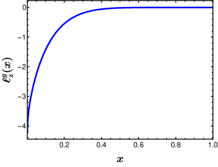
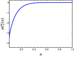
Figure 6: Model predictions for the gluon canonical OAM which can be obtained with $F_{1,4}^{g}$ gluon GTMD (Left) whereas the gluon spin-orbit correlations function which can be obtained with gluon $G_{1,1}^{g}$ GTMD (Right).

Similarly, the spin-orbit correlation factor for the gluons can be obtained by using the gluon GTMD $G_{1,1}^{g}$ as Chakrabarti et al. (2017); Lorce and Pasquini (2011); Maji et al. (2022); Gurjar et al. (2021),

$$C_{z}^{g}(x)=\int d^{2}{\bf p}_{\perp}\frac{{\bf p}_{\perp}^{2}}{M^{2}}G_{1,1}^{g}(x,0,{\bf p}_{\perp},0,0)$$ (41)

and the fourth chiral even GTMD $G_{1,4}^{g}$ gives the gluon helicity TMD $g_{1L}^{g}$ in the forward limit, corresponding collinear parton distribution is gluon helicity PDF which contributes to the proton spin as,

$$\Delta G=\int dxd^{2}{\bf p}_{\perp}G_{1,4}^{g}(x,0,{\bf p}_{\perp},0,0)$$ (42)

In Fig. 6 we show the gluon momentum fraction $x$ dependence of canonical orbital angular momentum in the left panel, whereas the spin-orbit correlation function has been depicted in the right panel. One can notice that the gluon canonical OAM, $\ell_{z}^{g}(x)$ and spin-orbit correlation factor $\mathcal{C}_{z}^{g}(x)$ both distributions have negative values in the whole range of $x$. After integrating $\ell_{z}^{g}(x)$ over $x$ one can obtain the numerical value of gluon canonical orbital angular momentum which gives the contribution into Jaffe–Manohar spin sum rule. In our model calculations, we obtained the numerical value of canonical OAM as $\ell_{z}^{g}=-0.38$, which is in good agreement with the another spectator model canonical OAM result, $\ell^{g}_{z}\simeq-0.333$ Tan and Lu (2023b). As similar to quarks, the canonical and kinetical gluon OAMs are comparable in our model, i.e., $\ell_{z}^{g}\sim L_{z}^{g}$ as reported in Refs. Lorce (2013); Ji et al. (2012); Leader and Lorcé (2014). The spin-orbit correlation factor is $c_{z}^{g}=-15.5$ in our model, the negative sign implies that the gluon spin and OAM are oriented in opposite directions.

V GPDs in impact parameter space (IPDs)

The two-dimensional Fourier transform of the GPDs at zero skewness with respect to the transverse momentum transferred, $\Delta_{\perp}$ to the process is used to determine the impact parameter-dependent generalized parton distributions, also known as IPDs Burkardt (2003),

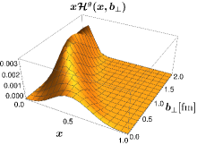
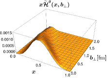
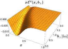
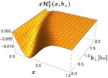
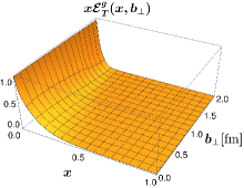
Figure 7: 3D plots of impact parameter dependent GPDs, $\mathcal{H}^{g}$, $\widetilde{\mathcal{H}}^{g}$, $\mathcal{E}^{g}$, $\mathcal{H}_{T}^{g}$ and $\mathcal{E}_{T}^{g}$ as a function of $x$ and the transverse impact parameter $b_{\perp}$ (in fm) at $\xi=0$.

$$\mathcal{F}(x,b_{\perp})=\int\frac{d^{2}\Delta_{\perp}}{(2\pi)^{2}}e^{-i\Delta_{\perp}.b_{\perp}}F^{g}(x,\xi=0,t=-\Delta_{\perp}^{2})$$ (43)

where $b_{\perp}$ is the impact parameter in the transverse plane which is the transverse distance between the struck parton and the center of momentum of the hadron. In the context of momentum space, the generalized parton distributions are depicted as off-diagonal matrix elements devoid of any immediate probabilistic implications. Conversely, when analyzed within the framework of impact parameter space, these distributions not only adhere to rigorous positivity conditions but also offer a compelling and substantial probabilistic interpretation Burkardt (2000, 2003).

In Figure 7, we depict three-dimensional representations of the non-zero generalized parton distributions in impact parameter space. Both the chiral even and the chiral odd GPDs are presented as functions of gluon longitudinal momentum fraction $x$ and impact parameter $b_{\perp}$ at zero skewness. Notably, the first plot in Figure 7 reveals that the impact parameter distribution $\mathcal{H}^{g}$ satisfies stringent positivity constraints, i.e., $\mathcal{H}^{g}\geq 0$, thereby affording a probabilistic interpretation. For a more precise understanding, one can examine the first plot in Figure 8, which illustrates how the unpolarized IPDs change with respect to the impact parameter $b_{\perp}$ at particular values of gluon momentum fraction $x$.

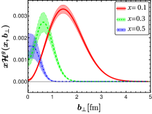
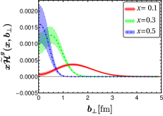
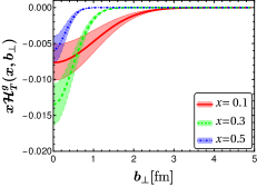
Figure 8: 2D plots of impact parameter dependent GPDs, $\mathcal{H}^{g}$, $\widetilde{\mathcal{H}}^{g}$, $\mathcal{E}^{g}$, $\mathcal{H}_{T}^{g}$ and $\mathcal{E}_{T}^{g}$ as a function of the transverse impact parameter $b_{\perp}$ (in fm) for specific values of the momentum fraction $x$, precisely, $x=0.1,~{}x=0.3~{}\text{and}~{}x=0.5$, with $\xi=0$.

Likewise, the helicity GPD in impact parameter space, $\widetilde{\mathcal{H}}^{g}$, exhibits a positive distribution across the entire transverse impact parameter range, adhering to the positivity constraint. This specific representation of the helicity GPD in impact parameter space quantifies the difference in density between gluons with positive and negative helicity. The generalized parton distributions $\mathcal{E}^{g}$ and $\mathcal{H}_{T}^{g}$ exhibit comparable shapes and display a negative distribution across the entire range of impact parameter space. To establish a probabilistic understanding, it is crucial to focus on amplitudes where the initial and final states possess matching helicities. Nevertheless, a challenge arises when attempting to develop a probabilistic interpretation for $E^{g}$ in momentum space, as it is associated with states that have differing helicities between the initial and final states. Finally, the chiral-odd GPD, denoted as $\mathcal{E}^{g}_{T}$, exhibits a positive behavior across the entire range of $b_{\perp}$. It demonstrates significant amplitude at small $x$ values but is noticeably attenuated in the region $x\geq 0.5$.

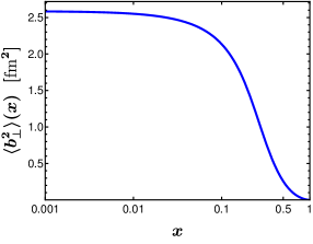
Figure 9: Model predictions for the average squared transverse radius of the gluon density, denoted as $\langle b^{2}_{\perp}\rangle$ (in fm²) as a function of $x$.

In Fig. 9 we present the squared radius of gluon densities in the transverse plane as a function of $x$. The parameter $\langle b_{\perp}^{2}\rangle$ signifies the transverse size of the hadron, revealing an expansion of the transverse radius as parton momentum fraction $x$ decreases Dupre et al. (2017). At lower values of $x$, the gluon displays a larger transverse average radii in contrast to the quark. Conversely, as $x$ values increase, the transverse size of the gluon decreases. As expected, when $x$ approaches to 1, the proton’s transverse size resembles that of a point-like object, illustrating the color transparency of the proton Brodsky and de Teramond (2022); Dupre et al. (2017).

VI conclusion

In this work, we have employed a recently developed light-front spectator model, incorporating the gluon as an active parton and the rest as a spectator. The proton light-front wavefunctions are adopted from the soft-wall AdS/QCD prediction. The model provides valuable insights into the leading twist gluon TMDPDFs, GPDs, and GTMDs. Within the light-cone formalism, the above distribution functions can be expressed as the overlap of the proton wave functions. We have extended our investigation to the gluon GPDs at zero and non-zero skewness in the DGLAP region, shedding light on their intricate behavior in various momentum configurations. We have explored both chiral even and chiral-odd gluon GPDs at leading twist. At non-zero skewness, among the eight leading-twist GPDs only six of them survive in our model in which unpolarized and helicity GPD exhibit oscillatory behavior, $E^{g}$, $\tilde{E}^{g}$ and $\tilde{H}_{T}^{g}$ show negative magnitude while $E_{T}^{g}$ shows the positive distribution in the entire range of $x$ and $\xi$. We have particularly focused on the $\xi=0$ behavior of the GPDs in the momentum and impact parameter space. We have evaluated the canonical and kinetic OAMs and the spin-orbit correlations of the gluons through GTMDs and GPDs in this model dominating the small $x$ regions. We found that the canonical and kinetic orbital angular momentums are negative in the entire range of $x$ and they are approximately close to each other, as $\ell_{z}^{g}\simeq-0.38$ and $L_{z}^{g}\simeq-0.42$ in our model. Using Ji’s spin sum rule we have also calculated the total angular momentum, $J_{z}^{g}=0.058$, which agrees with the BLFQ predictions. The spin-orbit correlations are also negative, indicating that the gluon spin and OAM are anti-aligned. Further, we have also computed the average transverse square radius, $\langle b_{\perp}^{2}\rangle^{g}$ as a function of gluon longitudinal momentum fraction $x$. As expected, the transverse size decreases with increasing $x$. As $x$ approaches 1, the transverse size of the proton diminishes, and it behaves like a point-like object. Our investigation has the potential to establish important theoretical limitations regarding gluon GPDs and angular momentum. However, to confirm these predictions, further experimental measurements are essential.

VII acknowledgement

A. M. would like to thank SERB MATRICS (MTR/2021/000103) for funding. The work of T. M. is supported by the Science and Engineering Research Board (SERB) through the SRG (Start-up Research Grant) of File No. SRG/2023/001093. The work of C. M. is supported by new faculty start up funding by the Institute of Modern Physics, Chinese Academy of Sciences, Grant No. E129952YR0. C. M. also thanks the Chinese Academy of Sciences Presidents International Fellowship Initiative for the support via Grants No. 2021PM0023.

Appendix A Appendix

The matrix elements $T^{g}_{i}$ for the chiral even GPDs are given by the following relations with the LFWFs:

$$T^{g}_{1} = \int\frac{d^{2}\textbf{p}_{\perp}}{16\pi^{3}}\Big{[}\psi_{+1+\frac{1}{2}}^{\uparrow\ast}\left(x^{\prime},{\bf p}_{\perp}^{\prime}\right)\psi_{+1+\frac{1}{2}}^{\uparrow}\left(x^{\prime\prime},{\bf p}_{\perp}^{\prime\prime}\right)+\psi_{+1-\frac{1}{2}}^{\uparrow\ast}\left(x^{\prime},{\bf p}_{\perp}^{\prime}\right)\psi_{+1-\frac{1}{2}}^{\uparrow}\left(x^{\prime\prime},{\bf p}_{\perp}^{\prime\prime}\right)$$ (44)

$$+ \psi_{+1+\frac{1}{2}}^{\downarrow\ast}\left(x^{\prime},{\bf p}_{\perp}^{\prime}\right)\psi_{+1+\frac{1}{2}}^{\downarrow}\left(x^{\prime\prime},{\bf p}_{\perp}^{\prime\prime}\right)+\psi_{+1-\frac{1}{2}}^{\downarrow\ast}\left(x^{\prime},{\bf p}_{\perp}^{\prime}\right)\psi_{+1-\frac{1}{2}}^{\downarrow}\left(x^{\prime\prime},{\bf p}_{\perp}^{\prime\prime}\right)\Big{]}$$

$$T^{g}_{2} = \int\frac{d^{2}\textbf{p}_{\perp}}{16\pi^{3}}\Big{[}\psi_{+1+\frac{1}{2}}^{\uparrow\ast}\left(x^{\prime},{\bf p}_{\perp}^{\prime}\right)\psi_{+1+\frac{1}{2}}^{\uparrow}\left(x^{\prime\prime},{\bf p}_{\perp}^{\prime\prime}\right)+\psi_{+1-\frac{1}{2}}^{\uparrow\ast}\left(x^{\prime},{\bf p}_{\perp}^{\prime}\right)\psi_{+1-\frac{1}{2}}^{\uparrow}\left(x^{\prime\prime},{\bf p}_{\perp}^{\prime\prime}\right)$$ (45)

$$- \psi_{+1+\frac{1}{2}}^{\downarrow\ast}\left(x^{\prime},{\bf p}_{\perp}^{\prime}\right)\psi_{+1+\frac{1}{2}}^{\downarrow}\left(x^{\prime\prime},{\bf p}_{\perp}^{\prime\prime}\right)-\psi_{+1-\frac{1}{2}}^{\downarrow\ast}\left(x^{\prime},{\bf p}_{\perp}^{\prime}\right)\psi_{+1-\frac{1}{2}}^{\downarrow}\left(x^{\prime\prime},{\bf p}_{\perp}^{\prime\prime}\right)\Big{]}$$

$$T^{g}_{3} = \int\frac{d^{2}\textbf{p}_{\perp}}{16\pi^{3}}\Big{[}\psi_{+1+\frac{1}{2}}^{\uparrow\ast}\left(x^{\prime},{\bf p}_{\perp}^{\prime}\right)\psi_{+1+\frac{1}{2}}^{\downarrow}\left(x^{\prime\prime},{\bf p}_{\perp}^{\prime\prime}\right)+\psi_{+1-\frac{1}{2}}^{\uparrow\ast}\left(x^{\prime},{\bf p}_{\perp}^{\prime}\right)\psi_{+1-\frac{1}{2}}^{\downarrow}\left(x^{\prime\prime},{\bf p}_{\perp}^{\prime\prime}\right)$$ (46)

$$+\psi_{-1+\frac{1}{2}}^{\uparrow\ast}\left(x^{\prime},{\bf p}_{\perp}^{\prime}\right)\psi_{-1+\frac{1}{2}}^{\downarrow}\left(x^{\prime\prime},{\bf p}_{\perp}^{\prime\prime}\right)+\psi_{-1-\frac{1}{2}}^{\uparrow\ast}\left(x^{\prime},{\bf p}_{\perp}^{\prime}\right)\psi_{-1-\frac{1}{2}}^{\downarrow}\left(x^{\prime\prime},{\bf p}_{\perp}^{\prime\prime}\right)\Big{]}$$

$$T^{g}_{4} = \int\frac{d^{2}\textbf{p}_{\perp}}{16\pi^{3}}\Big{[}\psi_{+1+\frac{1}{2}}^{\uparrow\ast}\left(x^{\prime},{\bf p}_{\perp}^{\prime}\right)\psi_{+1+\frac{1}{2}}^{\downarrow}\left(x^{\prime\prime},{\bf p}_{\perp}^{\prime\prime}\right)+\psi_{+1-\frac{1}{2}}^{\uparrow\ast}\left(x^{\prime},{\bf p}_{\perp}^{\prime}\right)\psi_{+1-\frac{1}{2}}^{\downarrow}\left(x^{\prime\prime},{\bf p}_{\perp}^{\prime\prime}\right)$$ (47)

$$-\psi_{-1+\frac{1}{2}}^{\uparrow\ast}\left(x^{\prime},{\bf p}_{\perp}^{\prime}\right)\psi_{-1+\frac{1}{2}}^{\downarrow}\left(x^{\prime\prime},{\bf p}_{\perp}^{\prime\prime}\right)-\psi_{-1-\frac{1}{2}}^{\uparrow\ast}\left(x^{\prime},{\bf p}_{\perp}^{\prime}\right)\psi_{-1-\frac{1}{2}}^{\downarrow}\left(x^{\prime\prime},{\bf p}_{\perp}^{\prime\prime}\right)\Big{]}$$

Likewise, the matrix elements $\tilde{T}^{g}_{i}$ for the chiral odd GPDs in terms of LFWFs could be expressed as following:

$$\widetilde{T}^{g}_{1} = \int\frac{d^{2}\textbf{p}_{\perp}}{16\pi^{3}}\Big{[}\psi_{+1+\frac{1}{2}}^{\uparrow\ast}\left(x^{\prime},{\bf p}_{\perp}^{\prime}\right)\psi_{-1+\frac{1}{2}}^{\downarrow}\left(x^{\prime\prime},{\bf p}_{\perp}^{\prime\prime}\right)+\psi_{+1-\frac{1}{2}}^{\uparrow\ast}\left(x^{\prime},{\bf p}_{\perp}^{\prime}\right)\psi_{-1-\frac{1}{2}}^{\downarrow}\left(x^{\prime\prime},{\bf p}_{\perp}^{\prime\prime}\right)$$ (48)

$$+ \psi_{+1+\frac{1}{2}}^{\downarrow\ast}\left(x^{\prime},{\bf p}_{\perp}^{\prime}\right)\psi_{-1+\frac{1}{2}}^{\uparrow}\left(x^{\prime\prime},{\bf p}_{\perp}^{\prime\prime}\right)+\psi_{+1-\frac{1}{2}}^{\downarrow\ast}\left(x^{\prime},{\bf p}_{\perp}^{\prime}\right)\psi_{-1-\frac{1}{2}}^{\uparrow}\left(x^{\prime\prime},{\bf p}_{\perp}^{\prime\prime}\right)\Big{]}$$

$$\widetilde{T}^{g}_{2} = \int\frac{d^{2}\textbf{p}_{\perp}}{16\pi^{3}}\Big{[}\psi_{+1+\frac{1}{2}}^{\uparrow\ast}\left(x^{\prime},{\bf p}_{\perp}^{\prime}\right)\psi_{-1+\frac{1}{2}}^{\downarrow}\left(x^{\prime\prime},{\bf p}_{\perp}^{\prime\prime}\right)+\psi_{+1-\frac{1}{2}}^{\uparrow\ast}\left(x^{\prime},{\bf p}_{\perp}^{\prime}\right)\psi_{-1-\frac{1}{2}}^{\downarrow}\left(x^{\prime\prime},{\bf p}_{\perp}^{\prime\prime}\right)$$ (49)

$$- \psi_{+1+\frac{1}{2}}^{\downarrow\ast}\left(x^{\prime},{\bf p}_{\perp}^{\prime}\right)\psi_{-1+\frac{1}{2}}^{\uparrow}\left(x^{\prime\prime},{\bf p}_{\perp}^{\prime\prime}\right)-\psi_{+1-\frac{1}{2}}^{\downarrow\ast}\left(x^{\prime},{\bf p}_{\perp}^{\prime}\right)\psi_{-1-\frac{1}{2}}^{\uparrow}\left(x^{\prime\prime},{\bf p}_{\perp}^{\prime\prime}\right)\Big{]}$$

$$\widetilde{T}^{g}_{3} = \int\frac{d^{2}\textbf{p}_{\perp}}{16\pi^{3}}\Big{[}\psi_{+1+\frac{1}{2}}^{\uparrow\ast}\left(x^{\prime},{\bf p}_{\perp}^{\prime}\right)\psi_{-1+\frac{1}{2}}^{\uparrow}\left(x^{\prime\prime},{\bf p}_{\perp}^{\prime\prime}\right)+\psi_{+1-\frac{1}{2}}^{\uparrow\ast}\left(x^{\prime},{\bf p}_{\perp}^{\prime}\right)\psi_{-1-\frac{1}{2}}^{\uparrow}\left(x^{\prime\prime},{\bf p}_{\perp}^{\prime\prime}\right)$$ (50)

$$+ \psi_{-1+\frac{1}{2}}^{\uparrow\ast}\left(x^{\prime},{\bf p}_{\perp}^{\prime}\right)\psi_{+1+\frac{1}{2}}^{\uparrow}\left(x^{\prime\prime},{\bf p}_{\perp}^{\prime\prime}\right)+\psi_{-1-\frac{1}{2}}^{\uparrow\ast}\left(x^{\prime},{\bf p}_{\perp}^{\prime}\right)\psi_{+1-\frac{1}{2}}^{\uparrow}\left(x^{\prime\prime},{\bf p}_{\perp}^{\prime\prime}\right)\Big{]}$$

$$\widetilde{T}^{g}_{4} = \int\frac{d^{2}\textbf{p}_{\perp}}{16\pi^{3}}\Big{[}\psi_{+1+\frac{1}{2}}^{\uparrow\ast}\left(x^{\prime},{\bf p}_{\perp}^{\prime}\right)\psi_{-1+\frac{1}{2}}^{\uparrow}\left(x^{\prime\prime},{\bf p}_{\perp}^{\prime\prime}\right)+\psi_{+1-\frac{1}{2}}^{\uparrow\ast}\left(x^{\prime},{\bf p}_{\perp}^{\prime}\right)\psi_{-1-\frac{1}{2}}^{\uparrow}\left(x^{\prime\prime},{\bf p}_{\perp}^{\prime\prime}\right)$$ (51)

$$- \psi_{-1+\frac{1}{2}}^{\uparrow\ast}\left(x^{\prime},{\bf p}_{\perp}^{\prime}\right)\psi_{+1+\frac{1}{2}}^{\uparrow}\left(x^{\prime\prime},{\bf p}_{\perp}^{\prime\prime}\right)-\psi_{-1-\frac{1}{2}}^{\uparrow\ast}\left(x^{\prime},{\bf p}_{\perp}^{\prime}\right)\psi_{+1-\frac{1}{2}}^{\uparrow}\left(x^{\prime\prime},{\bf p}_{\perp}^{\prime\prime}\right)\Big{]}$$

where, the arguments of the LFWFs in the above equations (44-51) we use the notations as

$$x^{\prime}=\frac{x-\xi}{1-\xi},\quad\quad\quad{\bf p}_{\perp}^{\prime}={\bf p}_{\perp}+(1-x^{\prime})\frac{\bf{\Delta}_{\perp}}{2},$$ (52)

for the active gluon longitudinal momentum fraction $(x^{\prime})$ and transverse momentum $(\mathbf{p}_{\perp}^{\prime})$ in the final proton state and,

$$x^{\prime\prime}=\frac{x+\xi}{1+\xi},\quad\quad\quad{\bf p}_{\perp}^{\prime\prime}={\bf p}_{\perp}-(1-x^{\prime\prime})\frac{\bf{\Delta}_{\perp}}{2}.$$ (53)

for gluon’s longitudinal momentum fraction $(x^{\prime\prime})$ and transverse momentum $(\mathbf{p}_{\perp}^{\prime\prime})$ in the initial proton state, respectively.

By employing the notion of the helicity amplitude $A_{\lambda^{\prime}\mu^{\prime},\lambda\mu}$ as stated in equation (9) and using the model expression for LFWFs, one can obtain the following form of matrix elements for chiral even and odd GPDs.

$$T_{1}^{g}(x^{\prime},x^{\prime\prime}) = N_{g}^{2}\Bigg{[}F_{2}(x^{\prime},x^{\prime\prime})\left\{\frac{1}{\mathcal{A}^{2}}+\left(\frac{\mathcal{B}^{2}}{4\mathcal{A}^{2}}-\frac{1}{4}(1-x^{\prime})(1-x^{\prime\prime})+(x^{\prime\prime}-x^{\prime})\frac{\mathcal{B}}{4\mathcal{A}}\right)\frac{Q^{2}}{\mathcal{A}}\right\}$$ (54)

$$\qquad\qquad\qquad\qquad\qquad\qquad\qquad\quad-F_{1}(x^{\prime},x^{\prime\prime})\frac{1}{\mathcal{A}}\Bigg{]}\exp\left[Q^{2}\left(\mathcal{C}+\frac{\mathcal{B}^{2}}{4\mathcal{A}}\right)\right],$$

$$T_{2}^{g}(x^{\prime},x^{\prime\prime}) = N_{g}^{2}\bigg{[}F_{3}(x^{\prime},x^{\prime\prime})\left\{\frac{1}{\mathcal{A}^{2}}+\left(\frac{\mathcal{B}^{2}}{4\mathcal{A}^{2}}-\frac{1}{4}(1-x^{\prime})(1-x^{\prime\prime})+(x^{\prime\prime}-x^{\prime})\frac{\mathcal{B}}{4\mathcal{A}}\right)\frac{Q^{2}}{\mathcal{A}}\right\}$$ (55)

$$\qquad\qquad\qquad\qquad\qquad\qquad\qquad\quad-F_{1}(x^{\prime},x^{\prime\prime})\frac{1}{\mathcal{A}}\bigg{]}\exp\left[Q^{2}\left(\mathcal{C}+\frac{\mathcal{B}^{2}}{4\mathcal{A}}\right)\right],$$

$$T_{3}^{g}(x^{\prime},x^{\prime\prime})=N_{g}^{2}\left[F_{4}(x^{\prime},x^{\prime\prime})\Big{\{}\frac{\mathcal{B}Q}{2\mathcal{A}^{2}}+\frac{Q}{2\mathcal{A}}(1-x^{\prime\prime})\Big{\}}-F_{5}(x^{\prime},x^{\prime\prime})\Big{\{}\frac{\mathcal{B}Q}{2\mathcal{A}^{2}}-\frac{Q}{2\mathcal{A}}(1-x^{\prime})\Big{\}}\right]\exp\Big{[}Q^{2}\Big{(}\mathcal{C}+\frac{\mathcal{B}^{2}}{4\mathcal{A}}\Big{)}\Big{]},$$ (56)

$$T_{4}^{g}(x^{\prime},x^{\prime\prime})=N_{g}^{2}\left[F_{4}(x^{\prime},x^{\prime\prime})\Big{\{}\frac{\mathcal{B}Q}{2\mathcal{A}^{2}}+\frac{Q}{2\mathcal{A}}(1-x^{\prime\prime})\Big{\}}+F_{5}(x^{\prime},x^{\prime\prime})\Big{\{}\frac{\mathcal{B}Q}{2\mathcal{A}^{2}}-\frac{Q}{2\mathcal{A}}(1-x^{\prime})\Big{\}}\right]\exp\Big{[}Q^{2}\Big{(}\mathcal{C}+\frac{\mathcal{B}^{2}}{4\mathcal{A}}\Big{)}\Big{]},$$ (57)

$$\widetilde{T}^{g}_{1}(x^{\prime},x^{\prime\prime})=N_{g}^{2}\bigg{[}\frac{F_{5}(x^{\prime},x^{\prime\prime})}{1-x^{\prime}}\Big{\{}\frac{\mathcal{B}Q}{2\mathcal{A}^{2}}-\frac{Q}{2\mathcal{A}}(1-x^{\prime})\Big{\}}-\frac{F_{4}(x^{\prime},x^{\prime\prime})}{1-x^{\prime\prime}}\Big{\{}\frac{\mathcal{B}Q}{2\mathcal{A}^{2}}+\frac{Q}{2\mathcal{A}}(1-x^{\prime\prime})\Big{\}}\bigg{]}\exp\Big{[}Q^{2}\Big{(}\mathcal{C}+\frac{\mathcal{B}^{2}}{4\mathcal{A}}\Big{)}\Big{]},$$ (58)

$$\widetilde{T}^{g}_{2}(x^{\prime},x^{\prime\prime})=\widetilde{T}^{g}_{1}(x^{\prime},x^{\prime\prime})$$ (59)

$$\widetilde{T}^{g}_{3}(x^{\prime},x^{\prime\prime}) = N_{g}^{2}\left(F_{6}(x^{\prime},x^{\prime\prime})-F_{7}(x^{\prime},x^{\prime\prime})\right)\exp\left[Q^{2}\left(\mathcal{C}+\frac{\mathcal{B}^{2}}{4\mathcal{A}}\right)\right]$$ (60)

$$\times\left\{\left(\frac{\mathcal{\mathcal{B}}^{2}}{4\mathcal{\mathcal{A}}^{2}}-\frac{1}{4}(1-x^{\prime})(1-x^{\prime\prime})+(x^{\prime\prime}-x^{\prime})\frac{\mathcal{B}}{4\mathcal{A}}\right)\frac{Q^{2}}{\mathcal{A}}\right\}$$

$$\widetilde{T}^{g}_{4}(x^{\prime},x^{\prime\prime}) = N_{g}^{2}\left(F_{6}(x^{\prime},x^{\prime\prime})+F_{7}(x^{\prime},x^{\prime\prime})\right)\exp\left[Q^{2}\left(\mathcal{C}+\frac{\mathcal{B}^{2}}{4\mathcal{A}}\right)\right]$$ (61)

$$\times\left\{\left(\frac{\mathcal{\mathcal{B}}^{2}}{4\mathcal{\mathcal{A}}^{2}}-\frac{1}{4}(1-x^{\prime})(1-x^{\prime\prime})+(x^{\prime\prime}-x^{\prime})\frac{\mathcal{B}}{4\mathcal{A}}\right)\frac{Q^{2}}{\mathcal{A}}\right\}$$

where $\mathcal{A},\mathcal{B}$ and $\mathcal{C}$ are defined as,

$$\mathcal{A} = \mathcal{A}^{g}(x^{\prime},x^{\prime\prime})=-\frac{1}{2\kappa^{2}}\left(\frac{\log(\frac{1}{1-x^{\prime}})}{x^{\prime 2}}+\frac{\log(\frac{1}{1-x^{\prime\prime}})}{x^{\prime\prime 2}}\right)$$

$$\mathcal{B} = \mathcal{B}^{g}(x^{\prime},x^{\prime\prime})=\frac{1}{2\kappa^{2}}\left(\frac{(1-x^{\prime})\log(\frac{1}{1-x^{\prime}})}{x^{\prime 2}}-\frac{(1-x^{\prime\prime})\log(\frac{1}{1-x^{\prime\prime}})}{x^{\prime\prime 2}}\right)$$

$$\mathcal{C} = \mathcal{C}^{g}(x^{\prime},x^{\prime\prime})=\frac{1}{2\kappa^{2}}\left(\frac{(1-x^{\prime})^{2}\log(\frac{1}{1-x^{\prime}})}{4x^{\prime 2}}+\frac{(1-x^{\prime\prime})^{2}\log(\frac{1}{1-x^{\prime\prime}})}{4x^{\prime\prime 2}}\right)$$ (62)

whereas the functions, $F_{i}$ are para as,

$$F_{1}(x^{\prime},x^{\prime\prime}) = \frac{2}{\kappa^{2}}\sqrt{\frac{\log(\frac{1}{1-x^{\prime}})}{x^{\prime}}\frac{\log(\frac{1}{1-x^{\prime\prime}})}{x^{\prime\prime}}}(x^{\prime}x^{\prime\prime})^{b}\left((1-x^{\prime})(1-x^{\prime\prime})\right)^{a}\left(M-\frac{M_{X}}{1-x^{\prime}}\right)\left(M-\frac{M_{X}}{1-x^{\prime\prime}}\right)$$

$$F_{2}(x^{\prime},x^{\prime\prime}) = \frac{2}{\kappa^{2}}\sqrt{\frac{\log(\frac{1}{1-x^{\prime}})}{x^{\prime}}\frac{\log(\frac{1}{1-x^{\prime\prime}})}{x^{\prime\prime}}}(x^{\prime}x^{\prime\prime})^{b}\left((1-x^{\prime})(1-x^{\prime\prime})\right)^{a}\left(\frac{1+(1-x^{\prime})(1-x^{\prime\prime})}{x^{\prime}x^{\prime\prime}(1-x^{\prime})(1-x^{\prime\prime})}\right)$$

$$F_{3}(x^{\prime},x^{\prime\prime}) = \frac{2}{\kappa^{2}}\sqrt{\frac{\log(\frac{1}{1-x^{\prime}})}{x^{\prime}}\frac{\log(\frac{1}{1-x^{\prime\prime}})}{x^{\prime\prime}}}(x^{\prime}x^{\prime\prime})^{b}\left((1-x^{\prime})(1-x^{\prime\prime})\right)^{a}\left(\frac{1-(1-x^{\prime})(1-x^{\prime\prime})}{x^{\prime}x^{\prime\prime}(1-x^{\prime})(1-x^{\prime\prime})}\right)$$

$$F_{4}(x^{\prime},x^{\prime\prime}) = \frac{2}{\kappa^{2}}\sqrt{\frac{\log(\frac{1}{1-x^{\prime}})}{x^{\prime}}\frac{\log(\frac{1}{1-x^{\prime\prime}})}{x^{\prime\prime}}}(x^{\prime}x^{\prime\prime})^{b}\left((1-x^{\prime})(1-x^{\prime\prime})\right)^{a}\frac{1}{x^{\prime\prime}}\left(M-\frac{M_{X}}{1-x^{\prime}}\right)$$

$$F_{5}(x^{\prime},x^{\prime\prime}) = \frac{2}{\kappa^{2}}\sqrt{\frac{\log(\frac{1}{1-x^{\prime}})}{x^{\prime}}\frac{\log(\frac{1}{1-x^{\prime\prime}})}{x^{\prime\prime}}}(x^{\prime}x^{\prime\prime})^{b}\left((1-x^{\prime})(1-x^{\prime\prime})\right)^{a}\frac{1}{x^{\prime}}\left(M-\frac{M_{X}}{1-x^{\prime\prime}}\right)$$

$$F_{6}(x^{\prime},x^{\prime\prime}) = \frac{2}{\kappa^{2}}\sqrt{\frac{\log(\frac{1}{1-x^{\prime}})}{x^{\prime}}\frac{\log(\frac{1}{1-x^{\prime\prime}})}{x^{\prime\prime}}}(x^{\prime}x^{\prime\prime})^{b}\left((1-x^{\prime})(1-x^{\prime\prime})\right)^{a}\frac{1}{x^{\prime\prime}x^{\prime}(1-x^{\prime})}$$

$$F_{7}(x^{\prime},x^{\prime\prime}) = \frac{2}{\kappa^{2}}\sqrt{\frac{\log(\frac{1}{1-x^{\prime}})}{x^{\prime}}\frac{\log(\frac{1}{1-x^{\prime\prime}})}{x^{\prime\prime}}}(x^{\prime}x^{\prime\prime})^{b}\left((1-x^{\prime})(1-x^{\prime\prime})\right)^{a}\frac{1}{x^{\prime}x^{\prime\prime}(1-x^{\prime\prime})}$$ (63)

References

• Müller et al. (1994) D. Müller, D. Robaschik, B. Geyer, F. M. Dittes, and J. Hořejši, Fortsch. Phys. 42, 101 (1994), eprint hep-ph/9812448.
• Diehl (2003) M. Diehl, Phys. Rept. 388, 41 (2003), eprint hep-ph/0307382.
• Belitsky and Radyushkin (2005) A. V. Belitsky and A. V. Radyushkin, Phys. Rept. 418, 1 (2005), eprint hep-ph/0504030.
• Goeke et al. (2001) K. Goeke, M. V. Polyakov, and M. Vanderhaeghen, Prog. Part. Nucl. Phys. 47, 401 (2001), eprint hep-ph/0106012.
• Boffi and Pasquini (2007) S. Boffi and B. Pasquini, Riv. Nuovo Cim. 30, 387 (2007), eprint 0711.2625.
• Brodsky et al. (2006) S. J. Brodsky, D. Chakrabarti, A. Harindranath, A. Mukherjee, and J. P. Vary, Phys. Lett. B 641, 440 (2006), eprint hep-ph/0604262.
• Meissner et al. (2009) S. Meissner, A. Metz, and M. Schlegel, JHEP 08, 056 (2009), eprint 0906.5323.
• Lorcé and Pasquini (2013) C. Lorcé and B. Pasquini, JHEP 09, 138 (2013), eprint 1307.4497.
• Kanazawa et al. (2014) K. Kanazawa, C. Lorcé, A. Metz, B. Pasquini, and M. Schlegel, Phys. Rev. D 90, 014028 (2014), eprint 1403.5226.
• Mukherjee et al. (2014) A. Mukherjee, S. Nair, and V. K. Ojha, Phys. Rev. D 90, 014024 (2014), eprint 1403.6233.
• Hagiwara et al. (2016) Y. Hagiwara, Y. Hatta, and T. Ueda, Phys. Rev. D 94, 094036 (2016), eprint 1609.05773.
• Ojha et al. (2023) V. K. Ojha, S. Jana, and T. Maji, Phys. Rev. D 107, 074040 (2023), eprint 2211.02959.
• Maji et al. (2022) T. Maji, C. Mondal, and D. Kang, Phys. Rev. D 105, 074024 (2022), eprint 2202.08635.
• Mukherjee et al. (2015) A. Mukherjee, S. Nair, and V. K. Ojha, Phys. Rev. D 91, 054018 (2015), eprint 1501.03728.
• More et al. (2018) J. More, A. Mukherjee, and S. Nair, Eur. Phys. J. C 78, 389 (2018), eprint 1709.00943.
• Chakrabarti et al. (2020a) D. Chakrabarti, N. Kumar, T. Maji, and A. Mukherjee, Eur. Phys. J. Plus 135, 496 (2020a), eprint 1902.07051.
• Maji et al. (2017) T. Maji, C. Mondal, and D. Chakrabarti, Phys. Rev. D 96, 013006 (2017), eprint 1702.02493.
• Zhang et al. (2023) Z. Zhang, Z. Hu, S. Xu, C. Mondal, X. Zhao, and J. P. Vary (2023), eprint 2312.00667.
• Ji (1997a) X.-D. Ji, Phys. Rev. D 55, 7114 (1997a), eprint hep-ph/9609381.
• Radyushkin (1997) A. V. Radyushkin, Phys. Rev. D 56, 5524 (1997), eprint hep-ph/9704207.
• Ji and Osborne (1998) X.-D. Ji and J. Osborne, Phys. Rev. D 58, 094018 (1998), eprint hep-ph/9801260.
• Ji (1998) X.-D. Ji, J. Phys. G 24, 1181 (1998), eprint hep-ph/9807358.
• Blumlein et al. (1999) J. Blumlein, B. Geyer, and D. Robaschik, Nucl. Phys. B 560, 283 (1999), eprint hep-ph/9903520.
• Guo et al. (2023a) Y. Guo, X. Ji, Y. Liu, and J. Yang, Phys. Rev. D 108, 034003 (2023a), eprint 2305.06992.
• Hackett et al. (2023) D. C. Hackett, P. R. Oare, D. A. Pefkou, and P. E. Shanahan (2023), eprint 2307.11707.
• Garcia Martin-Caro et al. (2023) A. Garcia Martin-Caro, M. Huidobro, and Y. Hatta, Phys. Rev. D 108, 034014 (2023), eprint 2304.05994.
• Burkert et al. (2023a) V. D. Burkert, L. Elouadrhiri, F. X. Girod, C. Lorcé, P. Schweitzer, and P. E. Shanahan (2023a), eprint 2303.08347.
• More et al. (2023) J. More, A. Mukherjee, S. Nair, and S. Saha, Phys. Rev. D 107, 116005 (2023), eprint 2302.11906.
• Choudhary et al. (2022) P. Choudhary, B. Gurjar, D. Chakrabarti, and A. Mukherjee, Phys. Rev. D 106, 076004 (2022), eprint 2206.12206.
• de Téramond et al. (2021) G. F. de Téramond, H. G. Dosch, T. Liu, R. S. Sufian, S. J. Brodsky, and A. Deur (HLFHS), Phys. Rev. D 104, 114005 (2021), eprint 2107.01231.
• Polyakov and Schweitzer (2018) M. V. Polyakov and P. Schweitzer, Int. J. Mod. Phys. A 33, 1830025 (2018), eprint 1805.06596.
• Lorcé et al. (2019) C. Lorcé, H. Moutarde, and A. P. Trawiński, Eur. Phys. J. C 79, 89 (2019), eprint 1810.09837.
• Chakrabarti et al. (2020b) D. Chakrabarti, C. Mondal, A. Mukherjee, S. Nair, and X. Zhao, Phys. Rev. D 102, 113011 (2020b), eprint 2010.04215.
• Mondal (2017) C. Mondal, Eur. Phys. J. C 77, 640 (2017), eprint 1709.06877.
• Li and Vary (2023) Y. Li and J. P. Vary (2023), eprint 2312.02543.
• Burkert et al. (2023b) V. D. Burkert, L. Elouadrhiri, and F. X. Girod (2023b), eprint 2310.11568.
• Singh et al. (2023) R. Singh, S. Saha, A. Mukherjee, and N. Mathur (2023), eprint 2311.04622.
• More et al. (2022) J. More, A. Mukherjee, S. Nair, and S. Saha, Phys. Rev. D 105, 056017 (2022), eprint 2112.06550.
• Burkardt (2003) M. Burkardt, Int. J. Mod. Phys. A 18, 173 (2003), eprint hep-ph/0207047.
• Burkardt (2006) M. Burkardt, Int. J. Mod. Phys. A 21, 926 (2006), eprint hep-ph/0509316.
• Adloff et al. (2000) C. Adloff et al. (H1), Eur. Phys. J. C 13, 371 (2000), eprint hep-ex/9902019.
• Airapetian et al. (2001) A. Airapetian et al. (HERMES), Phys. Rev. Lett. 87, 182001 (2001), eprint hep-ex/0106068.
• Adloff et al. (2001) C. Adloff et al. (H1), Phys. Lett. B 517, 47 (2001), eprint hep-ex/0107005.
• Aktas et al. (2005) A. Aktas et al. (H1), Eur. Phys. J. C 44, 1 (2005), eprint hep-ex/0505061.
• Aaron et al. (2009) F. D. Aaron et al. (H1), Phys. Lett. B 681, 391 (2009), eprint 0907.5289.
• Chekanov et al. (2003) S. Chekanov et al. (ZEUS), Phys. Lett. B 573, 46 (2003), eprint hep-ex/0305028.
• Airapetian et al. (2010) A. Airapetian et al. (HERMES), JHEP 08, 130 (2010), eprint 1002.3921.
• Airapetian et al. (2012a) A. Airapetian et al. (HERMES), JHEP 07, 032 (2012a), eprint 1203.6287.
• Airapetian et al. (2012b) A. Airapetian et al. (HERMES), JHEP 10, 042 (2012b), eprint 1206.5683.
• Abdul Khalek et al. (2022) R. Abdul Khalek et al., Nucl. Phys. A 1026, 122447 (2022), eprint 2103.05419.
• Lin et al. (2023) B. Lin, S. Nair, S. Xu, Z. Hu, C. Mondal, X. Zhao, and J. P. Vary (2023), eprint 2308.08275.
• Guo et al. (2022) Y. Guo, X. Ji, and K. Shiells, JHEP 09, 215 (2022), eprint 2207.05768.
• Mondal and Chakrabarti (2015) C. Mondal and D. Chakrabarti, Eur. Phys. J. C 75, 261 (2015), eprint 1501.05489.
• Lorce and Pasquini (2011) C. Lorce and B. Pasquini, Phys. Rev. D 84, 014015 (2011), eprint 1106.0139.
• Lorce et al. (2012) C. Lorce, B. Pasquini, X. Xiong, and F. Yuan, Phys. Rev. D 85, 114006 (2012), eprint 1111.4827.
• Bhattacharya et al. (2022) S. Bhattacharya, R. Boussarie, and Y. Hatta, Phys. Rev. Lett. 128, 182002 (2022), eprint 2201.08709.
• Ji (2003) X.-d. Ji, Phys. Rev. Lett. 91, 062001 (2003), eprint hep-ph/0304037.
• Belitsky et al. (2004) A. V. Belitsky, X.-d. Ji, and F. Yuan, Phys. Rev. D 69, 074014 (2004), eprint hep-ph/0307383.
• Ji et al. (2012) X. Ji, X. Xiong, and F. Yuan, Phys. Rev. Lett. 109, 152005 (2012), eprint 1202.2843.
• Hatta (2012) Y. Hatta, Phys. Lett. B 708, 186 (2012), eprint 1111.3547.
• Jaffe (1996) R. L. Jaffe, Phys. Lett. B 365, 359 (1996), eprint hep-ph/9509279.
• Adare et al. (2009) A. Adare et al. (PHENIX), Phys. Rev. Lett. 103, 012003 (2009), eprint 0810.0694.
• Boer et al. (2011) D. Boer et al. (2011), eprint 1108.1713.
• Bhattacharya et al. (2023a) S. Bhattacharya, R. Boussarie, and Y. Hatta, Acta Phys. Polon. Supp. 16, 7 (2023a).
• Bhattacharya et al. (2023b) S. Bhattacharya, D. Zheng, and J. Zhou (2023b), eprint 2304.05784.
• Gurjar et al. (2022) B. Gurjar, C. Mondal, and D. Chakrabarti (2022), eprint 2209.14285.
• Xu et al. (2022) S. Xu, C. Mondal, X. Zhao, Y. Li, and J. P. Vary (2022), eprint 2209.08584.
• Chakrabarti et al. (2023) D. Chakrabarti, P. Choudhary, B. Gurjar, R. Kishore, T. Maji, C. Mondal, and A. Mukherjee, Phys. Rev. D 108, 014009 (2023), eprint 2304.09908.
• Zhou et al. (2022) Y. Zhou, N. Sato, and W. Melnitchouk (Jefferson Lab Angular Momentum (JAM)), Phys. Rev. D 105, 074022 (2022), eprint 2201.02075.
• Abdallah et al. (2022) M. S. Abdallah et al. (STAR), Phys. Rev. D 105, 092011 (2022), eprint 2110.11020.
• Ji et al. (2021) X. Ji, F. Yuan, and Y. Zhao, Nature Rev. Phys. 3, 27 (2021), eprint 2009.01291.
• Yang et al. (2017) Y.-B. Yang, R. S. Sufian, A. Alexandru, T. Draper, M. J. Glatzmaier, K.-F. Liu, and Y. Zhao, Phys. Rev. Lett. 118, 102001 (2017), eprint 1609.05937.
• Sato et al. (2016) N. Sato, W. Melnitchouk, S. E. Kuhn, J. J. Ethier, and A. Accardi (Jefferson Lab Angular Momentum), Phys. Rev. D 93, 074005 (2016), eprint 1601.07782.
• de Florian et al. (2014) D. de Florian, R. Sassot, M. Stratmann, and W. Vogelsang, Phys. Rev. Lett. 113, 012001 (2014), eprint 1404.4293.
• Meissner et al. (2007) S. Meissner, A. Metz, and K. Goeke, Phys. Rev. D 76, 034002 (2007), eprint hep-ph/0703176.
• Leader and Lorcé (2014) E. Leader and C. Lorcé, Phys. Rept. 541, 163 (2014), eprint 1309.4235.
• Wakamatsu (2010) M. Wakamatsu, Phys. Rev. D 81, 114010 (2010), eprint 1004.0268.
• Ji (1997b) X.-D. Ji, Phys. Rev. Lett. 78, 610 (1997b), eprint hep-ph/9603249.
• Brodsky et al. (2001) S. J. Brodsky, D. S. Hwang, B.-Q. Ma, and I. Schmidt, Nucl. Phys. B 593, 311 (2001), eprint hep-th/0003082.
• Gutsche et al. (2014) T. Gutsche, V. E. Lyubovitskij, I. Schmidt, and A. Vega, Phys. Rev. D 89, 054033 (2014), [Erratum: Phys.Rev.D 92, 019902 (2015)], eprint 1306.0366.
• Brodsky et al. (2015) S. J. Brodsky, G. F. de Teramond, H. G. Dosch, and J. Erlich, Phys. Rept. 584, 1 (2015), eprint 1407.8131.
• Bacchetta et al. (2020) A. Bacchetta, F. G. Celiberto, M. Radici, and P. Taels, Eur. Phys. J. C 80, 733 (2020), eprint 2005.02288.
• Diehl (2001) M. Diehl, Eur. Phys. J. C 19, 485 (2001), eprint hep-ph/0101335.
• Guo et al. (2023b) Y. Guo, X. Ji, M. G. Santiago, K. Shiells, and J. Yang, JHEP 05, 150 (2023b), eprint 2302.07279.
• Guo et al. (2023c) Y. Guo, X. Ji, and F. Yuan (2023c), eprint 2308.13006.
• Diehl et al. (2001) M. Diehl, T. Feldmann, R. Jakob, and P. Kroll, Nucl. Phys. B 596, 33 (2001), [Erratum: Nucl.Phys.B 605, 647–647 (2001)], eprint hep-ph/0009255.
• Kriesten et al. (2022) B. Kriesten, P. Velie, E. Yeats, F. Y. Lopez, and S. Liuti, Phys. Rev. D 105, 056022 (2022), eprint 2101.01826.
• Tan and Lu (2023a) C. Tan and Z. Lu, Phys. Rev. D 108, 054038 (2023a), eprint 2301.09081.
• Alexandrou et al. (2020) C. Alexandrou, S. Bacchio, M. Constantinou, J. Finkenrath, K. Hadjiyiannakou, K. Jansen, G. Koutsou, H. Panagopoulos, and G. Spanoudes, Phys. Rev. D 101, 094513 (2020), eprint 2003.08486.
• Chen et al. (2008) X.-S. Chen, X.-F. Lu, W.-M. Sun, F. Wang, and T. Goldman, Phys. Rev. Lett. 100, 232002 (2008), eprint 0806.3166.
• Jaffe and Manohar (1990) R. L. Jaffe and A. Manohar, Nucl. Phys. B 337, 509 (1990).
• Ji et al. (2013) X. Ji, X. Xiong, and F. Yuan, Phys. Rev. D 88, 014041 (2013), eprint 1207.5221.
• Chakrabarti et al. (2017) D. Chakrabarti, T. Maji, C. Mondal, and A. Mukherjee, Phys. Rev. D 95, 074028 (2017), eprint 1701.08551.
• Gurjar et al. (2021) B. Gurjar, D. Chakrabarti, P. Choudhary, A. Mukherjee, and P. Talukdar, Phys. Rev. D 104, 076028 (2021), eprint 2107.02216.
• Tan and Lu (2023b) C. Tan and Z. Lu (2023b), eprint 2312.07997.
• Lorce (2013) C. Lorce, Phys. Lett. B 719, 185 (2013), eprint 1210.2581.
• Burkardt (2000) M. Burkardt, Phys. Rev. D 62, 071503 (2000), [Erratum: Phys.Rev.D 66, 119903 (2002)], eprint hep-ph/0005108.
• Dupre et al. (2017) R. Dupre, M. Guidal, and M. Vanderhaeghen, Phys. Rev. D 95, 011501 (2017), eprint 1606.07821.
• Brodsky and de Teramond (2022) S. J. Brodsky and G. F. de Teramond, MDPI Physics 4, 633 (2022), eprint 2202.13283.