On Lepton Flavor Violation and Dark Matter in Scotogenic model with Trimaximal Mixing

Abstract

We examine the Scotogenic model employing the TM₂ mixing matrix, $U_{\text{TM}_{2}}$, for neutrinos and parameterize the Yukawa coupling matrix $y$ based on the diagonalization condition for the neutrino mass matrix, $m_{\nu}$. Our investigation centers on analyzing the relic density of cold dark matter ($\Omega h^{2}$) and possible lepton flavor violation (LFV) in the model. While analyzing, we have taken into consideration respective experimental constraints on $\Omega h^{2}$ and LFV alongside neutrino oscillation data. In the second part, we have extended the analysis incorporating extended magic symmetry in $m_{\nu}$ enabling us to completely determine Yukawa coupling matrix ($y$). We observe a notable exclusion of the effective Majorana mass $|m_{ee}|$ parameter space by cosmological bound on sum of neutrino masses, particularly in the normal hierarchy while inverted hierarchy scenario is excluded due to constraints coming from extended magic symmetry. These findings shed light on the interplay among the Scotogenic model, TM₂ mixing, and extended magic symmetry, offering insights into the permitted parameter space and hierarchy exclusion.

1 Introduction

The experimental observations during the past two decades have affirmed our belief in the Standard Model (SM) of particle physics as the effective low energy theory explaining particle interactions at the fundamental level. Despite our present knowledge that neutrino has tiny mass and they mix while propagating in space, their theoretical origin is still not understood. Further, complete pattern of the neutrino mixing matrix is, also, unknown. Alongside observables in the neutrino sector, discerning cosmological dark matter (DM) and possible lepton flavor violation (LFV) emanating from underlying theory constitute formidable challenge in particle physics.

In this context, various extensions of the SM have been proposed to account, simultaneously, for non-zero neutrino mass and DM. Out of these extensions, the Scotogenic model stands as a theoretical framework in particle physics, providing a unified solution to two fundamental mysteries: the origin of neutrino masses and the existence of dark matter[1]. It was developed to address the puzzle of small neutrino masses and to offer insights into dark matter. In the Scotogenic model, neutrino masses arise at the 1-loop level, driven by quantum corrections involving new particles beyond the Standard Model. These additional particles, typically scalar or fermionic fields, interact with known particles in the Standard Model. The lightest of the $Z_{2}$ odd parity state is the possible DM particle in the model. In these models, the dark matter candidate originates from the same sector responsible for generating neutrino masses, establishing a natural connection between these phenomena[2, 3, 4, 5, 6, 7, 8, 9, 10, 11, 12, 13, 14, 15, 16, 17].

Meanwhile, the observation of a non-zero value for $\theta_{13}$ in various neutrino oscillation experiments has led to a reassessment of the Tribimaximal (TBM) mixing pattern[18, 19, 20, 21, 22, 23, 24] in light of experimental data [25, 26, 27, 28, 29, 30, 31, 32, 33, 34, 35, 36, 37, 38, 39, 40, 41, 42, 43, 44, 45, 46, 47, 48, 49, 50, 51, 52]. An alternative approach has emerged, preserving one column of the TBM mixing matrix while adjusting the remaining two to meet unitarity constraints. This adaptation results in three distinct trimaximal (TM) mixing patterns: TM₁, TM₂, and TM₃ [53, 54, 55, 56, 57, 58, 59, 60, 61, 62, 63, 64, 65, 66, 67, 68, 69, 71, 70, 72, 73, 74, 75], where the unchanged columns correspond to the first, second, and third positions within the TBM matrix, respectively. While the TM₃ configuration predicts $\theta_{13}$ to be zero, rendering it incompatible with observed data, both the TM₁ and TM₂ schemes have garnered significant attention for their ability to elucidate lepton mixing behaviors. The TM₂ scheme, in particular, aligns well with current neutrino oscillation data. Recent research has explored neutrino mass matrices incorporating TM₁ and TM₂ mixing frameworks with other phenomenological patterns of neutrino mass matrix, contributing to a deeper understanding of neutrino mixing phenomena[76, 77, 78, 79, 80, 81, 82, 83, 84, 85].

One of the key element in Scotogenesis is the structure of the Yukawa matrix ($y$) which is responsible for generating non-zero neutrino mass, possible LFV and contributes to relic density of the DM in the model. Alternative approaches have been employed in the literature to constrain its structure, based on (i) assuming specific parametrization of the Yukawa coupling matrix ($y$)[86] (ii) assuming appropriate patterns of the neutrino mixing matrix consistent with current neutrino oscillation data[90, 91, 87, 88, 89, 92, 93, 94, 95, 96], to name a few. It is pertinent to note that these approaches may have different predictions for observables like relic density of DM and LFV. Particularly, assuming an appropriate structure of neutrino mixing matrix may, further, constrain the allowed parameter space of the model satisfying observational constraints on neutrino oscillation parameters[97], LFV bounds[98, 99, 100, 101, 102, 103] and relic density of DM[104].

In this study, we investigate the relationship between neutrino physics and dark matter by employing TM₂ neutrino mixing matrix. The TM₂ mixing pattern result in magic neutrino mass matrix in which the sum of elements of each row/column is equal[105, 106, 107, 108, 109, 110, 111, 112]. We utilize the diagonalization condition of the flavor neutrino mass matrix to derive constraints on the elements of Yukawa coupling matrix ($y$). By integrating experimental constraints from both the neutrino sector and dark matter studies, we constrain the parameter space. We have, also, investigated the prediction of the model for possible LFV in $\mu\rightarrow e\gamma$ process on which we have the stringent experimental upper bound $\mathcal{O}(10^{-13})$[98]. Additionally, we incorporate the extended magic symmetry, proposed recently in Ref. [83], to refine our predictions. Our analysis indicates that the inverted hierarchy of neutrinos is not allowed under the constraint of the extended magic symmetry.

The paper is organized as follows: in Section 2, we have discussed the basic ingredients of the Scotogenic framework. In Section 3, we present analytical details of LFV and DM studies in the Scotogenic setup. In Section 4, we have discussed our formalism resulting in specific pattern of Yukawa coupling matrix ($y$) emanating from trimaximal mixing pattern (TM₂) of the neutrino mixing matrix. The numerical analysis and discussion is presented in Section 5. In Section 6, we extend our analysis to the extended magic symmetry case for both normal and inverted hierarchies of neutrino masses. Finally, we present conclusions of the present work in Section 7.

2 The Scotogenic Model

Among the myriad extensions proposed for the Standard Model (SM), the Scotogenic model [1] stands out for its unique capability to concurrently account for both neutrino mass and existence of dark matter. In its conventional form, the Scotogenic model encompasses the complete set of SM fields alongside three additional singlet Majorana fields, denoted as $N_{k}$ $(k=1,\,2,\,3)$, and an inert SU(2)_L scalar doublet, represented as $\zeta=$($\zeta^{+}$, $\zeta^{0}$), where $\zeta^{+}$ is charged component and $\zeta^{0}$ is the neutral component. From a symmetry perspective, in addition to the SM symmetry group (SU(3)${}_{C}\times$ SU(2)${}_{L}\times$U(1)_Y), the model introduces a new $Z_{2}$ symmetry. Under this exact $Z_{2}$ symmetry, all newly introduced fields possess odd parity, while all SM fields exhibit even parity viz.,

$$N_{k}\xrightarrow{}-N_{k},\,\,\,\zeta\xrightarrow{}-\zeta,\,\,\,\Phi\xrightarrow{}\Phi,\,\,\,\Psi_{\text{SM}}\xrightarrow{}\Psi_{\text{SM}},$$

where $\Psi_{\text{SM}}$ denotes all the SM fermions and $\Phi$ denotes SM Higgs doublet.

For the Scotogenic model, the relevant symmetry group comprises SU(2)${}_{L}\times$U(1)${}_{Y}\times$ $Z_{2}$. In the context of the lepton sector, the pertinent part of the Yukawa Lagrangian can be expressed as follows

$$-\mathcal{L}_{Y}=\Gamma_{\alpha\beta}\overline{L}_{\alpha}\Phi l_{R\beta}+y_{\alpha k}\overline{L}_{\alpha}\tilde{\zeta}N_{k}+\frac{1}{2}M_{k}\overline{N^{c}_{k}}N_{k}+\text{H.c.}\,\,,$$ (1)

where $\alpha$, $\beta=$ $e$, $\mu$, $\tau$ represent charged leptons, $M_{k}$ denote the mass of three Majorana singlet fermions $N_{k}$, $(k=1,\,2,\,3)$. The symbols $L_{\alpha}$ and $l_{R\beta}$ denote left-handed lepton doublets and right-handed lepton singlets, respectively, while $\Gamma_{\alpha\beta}$ and $y_{\alpha k}$ denote Yukawa couplings for charged leptons and neutrinos, respectively. Also, $\tilde{\zeta}=i\sigma_{2}\zeta^{*}$ where $\sigma_{2}$ is Pauli spin matrix and $N^{c}_{k}=C\overline{N_{k}}^{T}$, where $C$ is charge conjugation matrix.

The scalar potential under the exact $Z_{2}$ symmetry can be written as

$$\begin{split}V(\Phi,\zeta)=&\,\,\mu^{2}_{1}\Phi^{\dagger}\Phi+\mu^{2}_{2}\zeta^{\dagger}\zeta+\frac{1}{2}\lambda_{1}(\Phi^{\dagger}\Phi)^{2}+\frac{1}{2}\lambda_{2}(\zeta^{\dagger}\zeta)^{2}\\ &+\lambda_{3}(\Phi^{\dagger}\Phi)(\zeta^{\dagger}\zeta)+\lambda_{4}(\Phi^{\dagger}\zeta)(\zeta^{\dagger}\Phi)\\ &+\frac{1}{2}\lambda_{5}\big{[}(\Phi^{\dagger}\zeta)^{2}+\text{H.c.}\big{]}\,,\end{split}$$ (2)

where $\mu_{1}$, $\mu_{2}$, and $\lambda_{1}$ through $\lambda_{5}$ are real parameters.
As indicated by the imposed symmetry under $Z_{2}$, the presence of a term involving the Dirac Yukawa couplings of the $N_{k}$ with the SM Higgs doublet $\Phi$ is precluded. Additionally, since $\zeta$ is classified as an inert doublet, it does not acquire a vacuum expectation value (vev), thereby obstructing the generation of light neutrino mass at tree level through type-I seesaw mechanism. Consequently, neutrinos persist without acquiring mass at tree level. However, they can acquire mass through one-loop interactions, where the quartic term in the scalar potential assumes significance.

After electroweak symmetry breaking, the light neutrino mass generated at one-loop level can be expressed as

$$(m_{\nu})_{\alpha\beta}=\sum_{k=1}^{3}y_{\alpha k}y_{\beta k}\Lambda_{k}=(y\Lambda y^{T})_{\alpha\beta}\,,(\alpha,\beta=e,\mu,\tau).$$ (3)

In Eqn. (3), $y$ denotes the Yukawa coupling matrix which, in general, can be written as

$$y=\begin{pmatrix}y_{e1}&y_{e2}&y_{e3}\\ y_{\mu 1}&y_{\mu 2}&y_{\mu 3}\\ y_{\tau 1}&y_{\tau 2}&y_{\tau 3}\\ \end{pmatrix},$$ (4)

and $\Lambda=diag(\Lambda_{1},\Lambda_{2},\Lambda_{3})$, is the diagonal matrix with elements

$$\Lambda_{k}=\frac{\lambda_{5}v^{2}}{16\pi^{2}}\frac{1}{m_{0}}\frac{r_{k}}{1-r_{k}^{2}}\left(1-\frac{r_{k}^{2}}{1-r_{k}^{2}}\ln\frac{1}{r_{k}^{2}}\right),$$ (5)

where $r_{k}\equiv\frac{M_{k}}{m_{0}}$, $v$ is the vev of the SM Higgs doublet and $m_{0}^{2}=\frac{1}{2}(m_{R}^{2}+m_{I}^{2})$ where $m_{R}$ and $m_{I}$ denote masses of $\sqrt{2}\Re[\zeta^{0}]$ and $\sqrt{2}\Im[\zeta^{0}]$, respectively. It is to be noted that $\Lambda_{k}>0$ for $r_{k}\neq 1$. The radiatively generated neutrino masses will be small when we have $|\lambda_{5}|<<1$.

3 Lepton Flavor Violation and Coannihilation of Dark Matter

In the Scotogenic model, the exact $Z_{2}$ symmetry ensures that the lightest $Z_{2}$-odd particle remains stable, rendering it a viable candidate for dark matter. Thus, two scenarios emerge: the dark matter particle can either be a fermion or a neutral scalar. In the fermionic case, the lightest $Z_{2}$-odd particle would be the dark matter candidate, denoted as $N_{1}$. Alternatively, if the dark matter candidate is a neutral scalar, it would correspond to the component $\zeta^{0}$ of the inert doublet $\zeta$.

For the purpose of this study, we assume fermionic dark matter, implying that $N_{1}$ serves as the dark matter particle. This assumption sets the stage for investigating the properties and interactions of $N_{1}$ within the Scotogenic model framework.

Lepton flavor violation (LFV) is a phenomenon actively sought after in numerous experiments, with one of the most popular searches being for the radiative process $\mu\rightarrow e\gamma$. This process involves the rare decay of a muon into an electron and a photon, and its observation would provide crucial insights into physics beyond the Standard Model. In the Scotogenic model, this process induced at the one-loop level. The branching ratio of $\mu\rightarrow e\gamma$ is given by[113]

$$Br(\mu\rightarrow e\gamma)=\frac{3\alpha_{em}}{64\pi(G_{F}m_{0}^{2})^{2}}\left|\sum_{k=1}^{3}y_{\mu k}y_{ek}^{*}F(r_{k})\right|^{2}\,,$$ (6)

where $\alpha_{em}$ denotes the fine-structure constant, $G_{F}$ denotes the Fermi coupling constant, and loop function $F(r_{k})$ is defined by

$$F(r_{k})=\frac{1-6r_{k}^{2}+3r_{k}^{4}+2r_{k}^{6}-6r_{k}^{4}\ln r_{k}^{2}}{6(1-r_{k}^{2})^{4}}.$$ (7)

We aim to investigate both the relic density of cold dark matter (CDM) and the $\mu\rightarrow e\gamma$ process, but tension arises when considering a singlet fermion as a candidate for cold dark matter [113]. This tension arises because the same Yukawa couplings must satisfy experimental bounds for both processes, yet each process requires a different strength of the Yukawa couplings. This discrepancy poses a challenge in reconciling the requirements of both the relic density and the LFV process within the framework of a singlet fermion dark matter model.

To simultaneously study CDM and LFV within this model, considering the references [90, 91], it’s essential to recognize that when coannihilation effects are considered, the predicted CDM density and the branching ratio of the LFV process $\mu\rightarrow e\gamma$ can both align with observations. This alignment holds within the simplest Scotogenic model. Coannihilation necessitates nearly degenerate fermions. Thus, we assume $N_{1}$ and $N_{2}$ to be nearly degenerate, with $M_{1}\lesssim M_{2}<M_{3}$. This assumption facilitates the exploration of scenarios where coannihilation processes play a crucial role in both determining the relic density of CDM and influencing the LFV process $\mu\rightarrow e\gamma$.

Let $\sigma_{ij}$ $(i,j=1,2)$ be the annihilation cross section for the process $N_{i}N_{j}\rightarrow X\bar{X}$, where $X\,\text{and}\,\bar{X}$ represent a lepton and antilepton, respectively. Additionally, let $v_{rel}$ represents the relative velocity of the annihilation particles. Now, we can write the product of (co)annihilation cross section and relative velocity as[114]

$$\sigma_{ij}|v_{rel}|=a_{ij}+b_{ij}v^{2}_{rel},$$ (8)

where

$$a_{ij} = \frac{1}{8\pi m_{0}^{2}}\frac{r_{1}^{2}}{(r_{1}^{2}+1)^{2}}\sum_{\alpha\beta}\left|y_{\alpha i}y_{\beta j}^{*}-y_{\alpha j}^{*}y_{\beta i}\right|^{2},$$ (9)

$$b_{ij} = \frac{1-3r_{1}^{2}-r_{1}^{4}}{3(r_{1}^{2}+1)^{2}}a_{ij}+\frac{1}{12\pi}\frac{r_{1}^{2}(r_{1}^{4}+1)}{m_{0}^{2}(r_{1}^{2}+1)^{4}}\sum_{\alpha\beta}\left|y_{\alpha i}y_{\alpha j}^{*}y_{\beta i}y_{\beta j}^{*}\right|,$$ (10)

and effective cross section $\sigma_{eff}$ can be written as

$$\sigma_{eff} = \frac{g_{1}^{2}}{g_{eff}^{2}}\sigma_{11}+\frac{2g_{1}g_{2}}{g_{eff}^{2}}\sigma_{12}(1+\delta M)^{\frac{3}{2}}e^{-\delta Mx}+\frac{g_{2}^{2}}{g_{eff}^{2}}\sigma_{22}(1+\delta M)^{3}e^{-2\delta Mx},$$ (11)

$$g_{eff} = g_{1}+g_{2}(1+\delta M)^{\frac{3}{2}}e^{-\delta Mx},$$ (12)

where $g_{1}$ and $g_{2}$ denotes the number of degrees of freedom of the singlet fermions $N_{1}$ and $N_{2}$, respectively, $\delta M=(M_{2}-M_{1})/M_{1}$ denotes the mass splitting between the almost degenerate fermions $N_{1}$, and $N_{2}$ and $x=M_{1}/T$ denotes the ratio of dark matter particle mass to the temperature T. Since, we are considering coannihilation case in which $N_{1}$ and $N_{2}$ are nearly degenerate $\delta M\simeq 0$ and using Eqns. (8) and (12) in Eqn. (11), we have

$$\sigma_{eff}|v_{rel}| = \left(\frac{\sigma_{11}}{4}+\frac{\sigma_{12}}{2}+\frac{\sigma_{22}}{4}\right)|v_{rel}|\,,$$ (13)

$$= a_{eff}+b_{eff}v_{rel}^{2}\,,$$ (14)

where

$$a_{eff} = \frac{a_{11}}{4}+\frac{a_{12}}{2}+\frac{a_{22}}{4},$$ (15)

$$b_{eff} = \frac{b_{11}}{4}+\frac{b_{12}}{2}+\frac{b_{22}}{4}.$$ (16)

The thermally averaged cross section can be written as $\langle\sigma_{eff}|v_{rel}|\rangle$=$a_{eff}+6b_{eff}/x$ and the relic density of CDM is given by

$$\Omega h^{2}=\frac{1.07\times 10^{9}x_{f}}{g_{*}^{{1/2}}m_{\text{pl}}\text{(GeV)}(a_{eff}+3b_{eff}/x_{f})},$$ (17)

where $m_{\text{pl}}=1.22\times 10^{19}$ GeV is the Planck mass, $g_{*}=106.75$ is the total number of effectively relativistic degrees of freedom, and

$$x_{f}=\ln\frac{0.038g_{eff}m_{\text{pl}}M_{1}\langle\sigma_{eff}|v_{rel}|\rangle}{g_{*}^{1/2}x_{f}^{1/2}},$$ (18)

which is the value of $x$ at freeze-out temperature $T_{f}$.

4 Formalism

In our study, we recognize that the elements of the Yukawa coupling matrix are pivotal for determining both the branching ratio of LFV processes and the relic density of cold dark matter (CDM). Two common approaches for determining the Yukawa coupling matrix are available:

1. Casas-Ibarra (CI) Parametrization: This method, initially proposed in [86] and adapted to the Scotogenic model [115], involves parametrizing the Yukawa coupling matrix using CI parametrization. This approach offers a systematic way to link the neutrino sector with LFV processes and CDM relic density calculations.

2. Constraints from Diagonalization Condition of Neutrino Mass Matrix: Alternatively, one can use assumptions regarding the neutrino mixing matrix and apply the diagonalization condition of the flavor neutrino mass matrix to derive constraints on the Yukawa coupling matrix elements. This approach, extensively utilized in [90, 91, 87, 88, 89], involves expressing the Yukawa coupling matrix elements in terms of three independent Yukawa couplings. Further assumptions, such as texture zeros in the flavor neutrino mass matrix, can then be made to determine the values of these independent Yukawa couplings [92, 93, 95, 96, 94].

In this paper, we opt for the second method. We assume that mass matrix for charged leptons is diagonal. By leveraging constraints originating from the diagonalization condition of flavor neutrino mass matrix and assuming certain properties of the neutrino sector, such as texture zeros, we aim to determine the Yukawa coupling matrix elements and subsequently investigate their implications for both LFV processes and the relic density of CDM.

Among the various forms of the trimaximal mixing, we consider

$$U_{\text{TM}_{2}}=\begin{pmatrix}\sqrt{\frac{2}{3}}\cos\theta&\frac{1}{\sqrt{3}}&\sqrt{\frac{2}{3}}\sin\theta\\ -\frac{\cos\theta}{\sqrt{6}}+\frac{e^{-i\phi}\sin\theta}{\sqrt{2}}&\frac{1}{\sqrt{3}}&-\frac{\sin\theta}{\sqrt{6}}-\frac{e^{-i\phi}\cos\theta}{\sqrt{2}}\\ -\frac{\cos\theta}{\sqrt{6}}-\frac{e^{-i\phi}\sin\theta}{\sqrt{2}}&\frac{1}{\sqrt{3}}&-\frac{\sin\theta}{\sqrt{6}}+\frac{e^{-i\phi}\cos\theta}{\sqrt{2}}\\ \end{pmatrix},$$ (19)

where $\theta$ and $\phi$ are two free parameters. The neutrino mass matrix can be diagonalized by using the transformation

$$U^{T}_{\text{TM}_{2}}m_{\nu}U_{\text{TM}_{2}}=m_{\nu}^{d},$$ (20)

where $m_{\nu}^{d}=diag(m_{1},m_{2},m_{3})$ is diagonal neutrino mass matrix with eigenvalues $m_{i}$ ($i=1,2,3$). Substituting Eqns. (3) and (19) in Eqn. (20), and by requiring the equality in Eqn. (20) to hold, we have set of six equations, three for off-diagonal elements and three for diagonal elements. For simplicity, we have assumed $m^{\nu n}=U^{T}_{\text{TM}_{2}}m_{\nu}U_{\text{TM}_{2}}$. The three equations for off-diagonal elements are

$$m^{\nu n}_{12} = \sum_{i=1}^{3}\left[\sqrt{2}(2y_{ei}-y_{\mu i}-y_{\tau i})\cos\theta-\sqrt{6}e^{-i\phi}(y_{\tau i}-y_{\mu i})\sin\theta\right](y_{ei}+y_{\mu i}+y_{\tau i})\Lambda_{i}=0\,,$$ (21)

$$m^{\nu n}_{13} = \sum_{i=1}^{3}\left[\sqrt{3}e^{i\phi}(2y_{ei}-y_{\mu i}-y_{\tau i})(y_{\tau i}-y_{\mu i})\cos 2\theta-\frac{3}{2}(y_{\tau i}-y_{\mu i})^{2}\sin 2\theta+\frac{1}{2}e^{2i\phi}(2y_{ei}-y_{\mu i}-y_{\tau i})^{2}\sin 2\theta\right]\Lambda_{i}=0\,,$$ (22)

$$m^{\nu n}_{23} = \sum_{i=1}^{3}\left[\sqrt{6}e^{-i\phi}(y_{\tau i}-y_{\mu i})\cos\theta+\sqrt{2}(2y_{ei}-y_{\mu i}-y_{\tau i})\sin\theta\right](y_{ei}+y_{\mu i}+y_{\tau i})\Lambda_{i}=0\,,$$ (23)

and three equations for diagonal elements are

$$m^{\nu n}_{11} = \sum_{i=1}^{3}\frac{1}{6}\left[(2y_{ei}-y_{\mu i}-y_{\tau i})^{2}\cos^{2}\theta+3e^{-2i\phi}(y_{\tau i}-y_{\mu i})^{2}\sin^{2}\theta-\sqrt{3}e^{-i\phi}(y_{\tau i}-y_{\mu i})(2y_{ei}-y_{\mu i}-y_{\tau i})\sin 2\theta\right]\Lambda_{i}=m_{1}\,,$$ (24)

$$m^{\nu n}_{22} = \sum_{i=1}^{3}\frac{1}{3}(y_{ei}+y_{\mu i}+y_{\tau i})^{2}\Lambda_{i}=m_{2}\,,$$ (25)

$$m^{\nu n}_{33} = \sum_{i=1}^{3}\frac{1}{6}\left[(2y_{ei}-y_{\mu i}-y_{\tau i})^{2}\sin^{2}\theta+3e^{-2i\phi}(y_{\tau i}-y_{\mu i})^{2}\cos^{2}\theta+\sqrt{3}e^{-i\phi}(y_{\tau i}-y_{\mu i})(2y_{ei}-y_{\mu i}-y_{\tau i})\sin 2\theta\right]\Lambda_{i}=m_{3}\,.$$ (26)

With nine Yukawa couplings and six equations, we find ourselves with three Yukawa couplings that remain independent. We opt to set them as $y_{ei}=y_{i}$ for $i=1,2,3$ . Multiplying Eqn. (21) by $\cos\theta$ and Eqn. (23) by $\sin\theta$ and adding both of them, we have

$$\sum_{i=1}^{3}(2y_{ei}-y_{\mu i}-y_{\tau i})(y_{ei}+y_{\mu i}+y_{\tau i})=0.$$ (27)

Now, we have two solutions: either $(2y_{ei}-y_{\mu i}-y_{\tau i})=0$ or $(y_{ei}+y_{\mu i}+y_{\tau i})=0$. We substitute these solutions in Eqn. (22) and we obtain following results:

1. If $(2y_{ei}-y_{\mu i}-y_{\tau i})=0$, then

   $$y_{ei}=y_{\mu i}=y_{\tau i}.$$ (28)

2. If $(y_{ei}+y_{\mu i}+y_{\tau i})=0$, solving this equation with Eqn. (22) simultaneously for $y_{\mu i}$ and $y_{\tau i}$, we again have two solutions:

   1. $$\begin{rcases}y_{\mu i}=&\frac{1}{2}\left[-1+\sqrt{3}\cot 2\theta(-e^{i\phi}+e^{i\phi}\sec 2\theta)\right]y_{ei}\,,\\ y_{\tau i}=&\frac{1}{2}\left[-1-\sqrt{3}\cot 2\theta(-e^{i\phi}+e^{i\phi}\sec 2\theta)\right]y_{ei}\,,\end{rcases}$$ (29)

   2. $$\begin{rcases}y_{\mu i}=&\frac{1}{2}\left[-1-\sqrt{3}\cot 2\theta(e^{i\phi}+e^{i\phi}\sec 2\theta)\right]y_{ei}\,,\\ y_{\tau i}=&\frac{1}{2}\left[-1+\sqrt{3}\cot 2\theta(e^{i\phi}+e^{i\phi}\sec 2\theta)\right]y_{ei}\,.\end{rcases}$$ (30)

It is to be noted that we can independently choose any of these solutions for each value of $i\,(i=1,\,2,\,3)$. As all off-diagonal elements vanish with any of these solution sets, we can now determine the solutions for the diagonal elements that satisfy these conditions. The various choices of solution sets will result in different values for the three diagonal equations. In total, we can derive 27 sets of solutions. Among these, 3 sets yield two zero neutrino masses, 18 sets result in one zero neutrino mass, and the remaining 6 sets produce three non-zero neutrino masses.

Assuming that the mass eigenvalues $m_{i}$ ($i=1,\,2,\,3$) are all non-zero for our analysis, we have selected one of the 6 sets that provides non-zero values for all three neutrino masses. A similar analytical approach can be applied to the other solution sets. We can derive the following solution based on the our choices of solution for each $i$:

1. For $i=2$, we choose solution shown in Eqn. (28).

2. For $i=1$, we choose solution given by Eqn. (29) and for $i=3$, we choose solution given by Eqn. (30).

So, the Yukawa coupling matrix parameterized in terms of $y_{ei}=y_{i}$ ($i=1,2,3$) is given by

$$y=\begin{pmatrix}y_{1}&y_{2}&y_{3}\\ a_{1}y_{1}&y_{2}&a_{3}y_{3}\\ a_{2}y_{1}&y_{2}&a_{4}y_{3}\\ \end{pmatrix},$$ (31)

where

$$a_{1} = \frac{1}{2}\left[-1+\sqrt{3}\cot 2\theta(-e^{i\phi}+e^{i\phi}\sec 2\theta)\right],$$ (32)

$$a_{2} = \frac{1}{2}\left[-1-\sqrt{3}\cot 2\theta(-e^{i\phi}+e^{i\phi}\sec 2\theta)\right],$$ (33)

$$a_{3} = \frac{1}{2}\left[-1-\sqrt{3}\cot 2\theta(e^{i\phi}+e^{i\phi}\sec 2\theta)\right],$$ (34)

$$a_{4} = \frac{1}{2}\left[-1+\sqrt{3}\cot 2\theta(e^{i\phi}+e^{i\phi}\sec 2\theta)\right],$$ (35)

and neutrino mass eigenvalues are given by

$$m_{1}=c_{1}y_{1}^{2}\Lambda_{1},\,\,\ m_{2}=c_{2}y_{2}^{2}\Lambda_{2},\,\,\ m_{3}=c_{3}y_{3}^{2}\Lambda_{3},$$ (36)

where $c_{1}=\frac{3}{2}\sec^{2}\theta,c_{2}=3,c_{3}=\frac{3}{2}\csc^{2}\theta$ and $\Lambda_{1}\approx\Lambda_{2}.$ As Yukawa couplings are in general complex, we can write $y^{2}_{1}=|y^{2}_{1}|e^{i2\alpha_{1}}$, $y^{2}_{2}=|y^{2}_{2}|e^{i2\alpha_{2}}$ and $y^{2}_{3}=|y^{2}_{3}|e^{i2\alpha_{3}}$ which implies $y_{i}=\sqrt{|y^{2}_{i}|}e^{i\alpha_{i}}$, where $\alpha_{i}\,\,(i=1,2,3)$ are three Majorana phases. So, we have

$$m_{1}=|c_{1}y_{1}^{2}\Lambda_{1}|e^{i2\alpha_{1}},\,\,\ m_{2}=|c_{2}y_{2}^{2}\Lambda_{2}|e^{i2\alpha_{2}},\,\,\ m_{3}=|c_{3}y_{3}^{2}\Lambda_{3}|e^{i2\alpha_{3}}.$$ (37)

So, we get real and positive masses as

$$|m_{1}|=|c_{1}y_{1}^{2}\Lambda_{1}|,\,\,\ |m_{2}|=|c_{2}y_{2}^{2}\Lambda_{2}|,\,\,\ |m_{3}|=|c_{3}y_{3}^{2}\Lambda_{3}|.$$ (38)

Further these masses need to satisfy mass-squared differences given by

$$\Delta m^{2}_{21} = |m_{2}|^{2}-|m_{1}|^{2},$$ (39)

$$|\Delta m^{2}_{31}| = ||m_{3}|^{2}-|m_{1}|^{2}|,$$ (40)

where $\Delta m^{2}_{31}$ is positive for normal hierarchy (NH) and negative for inverted hierarchy (IH) of neutrinos. We can write three mass eigenvalues in terms of lightest neutrino mass. For NH, we have

$$|m_{2}| = \sqrt{\Delta m^{2}_{21}+|m_{1}|^{2}},$$ (41)

$$|m_{3}| = \sqrt{\Delta m^{2}_{31}+|m_{1}|^{2}},$$ (42)

and we can write the $y_{2}$ and $y_{3}$ in terms of $y_{1}$ as

$$|y_{2}^{2}| = \frac{1}{|c_{2}\Lambda_{1}|}\sqrt{\Delta m^{2}_{21}+|c_{1}y_{1}^{2}\Lambda_{1}|^{2}},$$

$$y_{2} = \sqrt{\frac{1}{|c_{2}\Lambda_{1}|}\sqrt{\Delta m^{2}_{21}+|c_{1}y_{1}^{2}\Lambda_{1}|^{2}}}e^{i\alpha_{2}},$$ (43)

and

$$|y_{3}^{2}| = \frac{1}{|c_{3}\Lambda_{3}|}\sqrt{\Delta m^{2}_{31}+|c_{1}y_{1}^{2}\Lambda_{1}|^{2}},$$

$$y_{3} = \sqrt{\frac{1}{|c_{3}\Lambda_{3}|}\sqrt{\Delta m^{2}_{31}+|c_{1}y_{1}^{2}\Lambda_{1}|^{2}}}e^{i\alpha_{3}}.$$ (44)

Here, we left with only one independent Yukawa coupling $y_{1}$ for the NH case. For the IH case, we have

$$|m_{1}| = \sqrt{\Delta m^{2}_{31}+|m_{3}|^{2}},$$ (45)

$$|m_{2}| = \sqrt{\Delta m^{2}_{21}+\Delta m^{2}_{31}+|m_{3}|^{2}}.$$ (46)

We can write the $y_{1}$ and $y_{2}$ in terms of $y_{3}$ as

$$|y_{1}^{2}| = \frac{1}{|c_{1}\Lambda_{1}|}\sqrt{\Delta m^{2}_{31}+|c_{3}y_{3}^{2}\Lambda_{3}|^{2}},$$

$$y_{1} = \sqrt{\frac{1}{|c_{1}\Lambda_{1}|}\sqrt{\Delta m^{2}_{31}+|c_{3}y_{3}^{2}\Lambda_{3}|^{2}}}e^{i\alpha_{1}},$$ (47)

and

$$|y_{2}^{2}| = \frac{1}{|c_{2}\Lambda_{1}|}\sqrt{\Delta m^{2}_{21}+\Delta m^{2}_{31}+|c_{3}y_{3}^{2}\Lambda_{3}|^{2}},$$

$$y_{2} = \sqrt{\frac{1}{|c_{2}\Lambda_{1}|}\sqrt{\Delta m^{2}_{21}+\Delta m^{2}_{31}+|c_{3}y_{3}^{2}\Lambda_{3}|^{2}}}e^{i\alpha_{2}}.$$ (48)

So, for the IH case, we are left with only one independent Yukawa coupling $y_{3}$. Using Eqn. (31) in Eqn. (3), the resulting neutrino mass matrix $m_{\nu}$ can be written as

$$m_{\nu}=\begin{pmatrix}y_{1}^{2}\Lambda_{1}+y_{2}^{2}\Lambda_{2}+y_{3}^{2}\Lambda_{3}&a_{1}y_{1}^{2}\Lambda_{1}+y_{2}^{2}\Lambda_{2}+a_{3}y_{3}^{2}\Lambda_{3}&a_{2}y_{1}^{2}\Lambda_{1}+y_{2}^{2}\Lambda_{2}+a_{4}y_{3}^{2}\Lambda_{3}\\ a_{1}y_{1}^{2}\Lambda_{1}+y_{2}^{2}\Lambda_{2}+a_{3}y_{3}^{2}\Lambda_{3}&a_{1}^{2}y_{1}^{2}\Lambda_{1}+y_{2}^{2}\Lambda_{2}+a_{3}^{2}y_{3}^{2}\Lambda_{3}&a_{1}a_{2}y_{1}^{2}\Lambda_{1}+y_{2}^{2}\Lambda_{2}+a_{3}a_{4}y_{3}^{2}\Lambda_{3}\\ a_{2}y_{1}^{2}\Lambda_{1}+y_{2}^{2}\Lambda_{2}+a_{4}y_{3}^{2}\Lambda_{3}&a_{1}a_{2}y_{1}^{2}\Lambda_{1}+y_{2}^{2}\Lambda_{2}+a_{3}a_{4}y_{3}^{2}\Lambda_{3}&a_{2}^{2}y_{1}^{2}\Lambda_{1}+y_{2}^{2}\Lambda_{2}+a_{4}^{2}y_{3}^{2}\Lambda_{3}\\ \end{pmatrix}.$$ (49)

By using the properties $a_{1}+a_{2}=-1$, $a_{3}+a_{4}=-1$, $a_{1}+a_{1}^{2}+a_{1}a_{2}=0$, $a_{2}+a_{2}^{2}+a_{1}a_{2}=0$, $a_{3}+a_{3}^{2}+a_{3}a_{4}=0$ and $a_{4}+a_{4}^{2}+a_{3}a_{4}=0$ (see Eqns. (32) to (35)), we can clearly see that this matrix is magic i.e. the sum of the elements in each row and column is equal to $c_{2}y_{2}^{2}\Lambda_{2}$ i.e., $m_{2}$.

In the upcoming sections (Sections 5 and 6), we shall explore two scenarios. In the first scenario (Section 5), we will investigate the implications of trimaximal mixing matrix on both LFV process ($\mu\rightarrow e\gamma$) and the relic density of CDM while simultaneously satisfying neutrino oscillation data, within Scotogenic model of neutrino mass generation. In the second scenario (Section 6), motivated from our earlier work[83], we shall introduce additional constraint on $m_{\nu}$, enabling us to determine independent Yukawa coupling ($y_{1}$ $(y_{3})$ for NH (IH)).

5 Numerical Analysis and Discussion

In the previous section, we have determined the structure of the Yukawa coupling matrix $y$ and the neutrino mass matrix $m_{\nu}$ emanating from TM₂ mixing paradigm. In this section, we will numerically investigate the neutrino phenomenology arising from this model and its implications for the relic density of cold dark matter ($\Omega h^{2}$) and possible LFV considering branching ratio of $\mu\rightarrow e\gamma$ process (Br($\mu\rightarrow e\gamma$)). For this study, we vary the neutrino mass-squared differences within their $3\sigma$ range [97], viz. $\Delta m_{21}^{2}=(6.94\,\,-\,\,8.14)\times 10^{-5}\text{eV}^{2}$ and $\Delta m_{31}^{2}=(2.47\,\,-\,\,2.63)\times 10^{-3}\text{eV}^{2}$ for normal hierarchy (NH), and $\Delta m_{31}^{2}=(2.37\,\,-\,\,2.53)\times 10^{-3}\text{eV}^{2}$ for inverted hierarchy (IH) (the negative sign is already included in our analysis, so $\Delta m_{31}^{2}$ for IH is taken as positive).

For the parameters originating from the Scotogenic model, we must ensure that $|\lambda_{5}|<<1$ for small neutrino masses, and for our choice of fermionic dark matter, $N_{1}$ will be the lightest, so we must have $M_{1}\lesssim M_{2}<M_{3}$, $M_{1}<m_{0}$, and $r_{1}<r_{3}$. Taking these into account, we randomly vary these parameters with a uniform distribution within the specified ranges, as shown in Table 1. Additionally, the free parameters $\theta$ and $\phi$, parametrizing TM₂ mixing matrix, are randomly varied in the range $0$ to $2\pi$ with uniform distribution.

Before proceeding further, let us write down some important relations used to obtain the physical observable parameters. In term of the elements of TM₂ mixing matrix (Eqn. (19)), neutrino mixing angles are obtained as

$$\begin{rcases}\begin{aligned} &\sin^{2}\theta_{12}=\frac{|(U_{\text{TM}_{2}})_{12}|^{2}}{1-|(U_{\text{TM}_{2}})_{13}|^{2}}=\frac{1}{\cos 2\theta+2},\\ &\sin^{2}\theta_{13}=|(U_{\text{TM}_{2}})_{13}|^{2}=\frac{2\sin^{2}\theta}{3},\\ &\sin^{2}\theta_{23}=\frac{|(U_{\text{TM}_{2}})_{23}|^{2}}{1-|(U_{\text{TM}_{2}})_{13}|^{2}}=\frac{1}{2}\left(\frac{\sqrt{3}\sin 2\theta\cos\phi}{\cos 2\theta+2}+1\right).\end{aligned}\end{rcases}$$ (50)

In our analysis we have considered Yukawa coupling matrix $y$ to be complex. Hence using Eqn. (37), three Majorana phases can be obtained as

$$\alpha_{1}=\frac{1}{2}\text{arg}[m_{1}],\,\,\ \alpha_{2}=\frac{1}{2}\text{arg}[m_{2}],\,\,\ \alpha_{3}=\frac{1}{2}\text{arg}[m_{3}].$$ (51)

Using these relations, we obtain two physical Majorana phases as

$$\alpha_{21}=\alpha_{2}-\alpha_{1},\,\,\ \alpha_{31}=\alpha_{3}-\alpha_{1}.$$ (52)

The Jarlskog $CP$ invariant[116, 117, 118], Dirac phase $\delta$, and other two invariants corresponding to Majorana phases $\alpha_{21}$ and $\alpha_{31}$ [119, 120, 122, 121] are given by

$$\begin{rcases}&J_{CP}=\text{Im}[(U_{\text{TM}_{2}})_{11}(U_{\text{TM}_{2}})_{12}^{*}(U_{\text{TM}_{2}})_{21}^{*}(U_{\text{TM}_{2}})_{22}]=\frac{1}{6\sqrt{3}}\sin 2\theta\sin\phi,\\ &\delta=\text{arc}\sin\left[\frac{J_{CP}}{\sin\theta_{12}\cos\theta_{12}\sin\theta_{23}\cos\theta_{23}\sin\theta_{13}\cos^{2}\theta_{13}}\right],\\ &I_{1}=\text{Im}[(U_{\text{TM}_{2}})_{11}^{*}(U_{\text{TM}_{2}})_{12}e^{i\alpha_{21}}]=\frac{\sqrt{2}}{3}\cos\theta\sin\alpha_{21},\\ &I_{2}=\text{Im}[(U_{\text{TM}_{2}})_{11}^{*}(U_{\text{TM}_{2}})_{13}e^{i\alpha_{31}}]=\frac{1}{3}\sin 2\theta\sin\alpha_{31}.\end{rcases}$$ (53)

The effective Majorana mass, denoted as $|m_{ee}|=|(m_{v})_{11}|=\left|\sum_{i=1}^{3}(U_{\text{TM}_{2}})^{2}_{1i}m_{i}\right|$, is a crucial observable in neutrinoless double beta decay ($0\nu\beta\beta$) experiments, which aim to establish the Majorana nature of neutrinos.

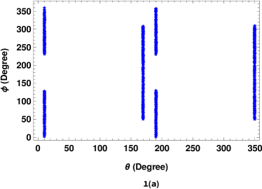
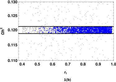
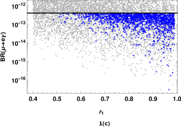
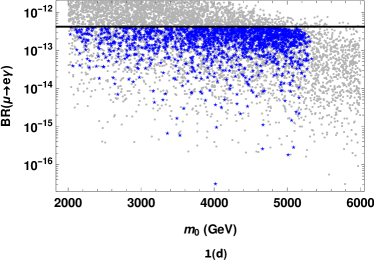
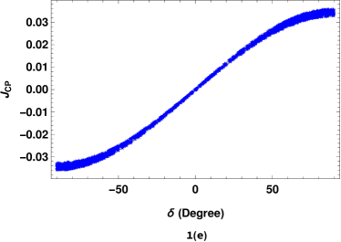
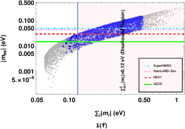
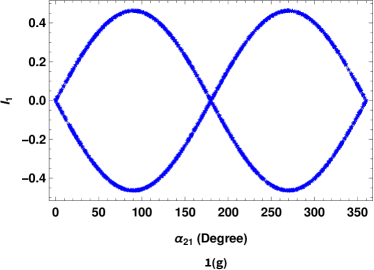
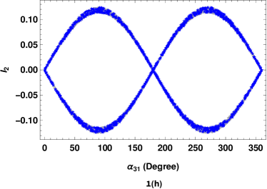
Figure 1: For NH of neutrino masses: the grey points show the parameter space that satisfies neutrino oscillation data at $3\sigma$, while the points shown in blue color (“$\filledstar$”) satisfy the simultaneity condition. The horizontal lines in Fig. 1(b) are experimental range of $\Omega h^{2}$. The horizontal line, in Figs. 1(c) and 1(d), represents experimental upper bound on Br($\mu\rightarrow e\gamma$).

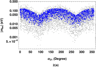
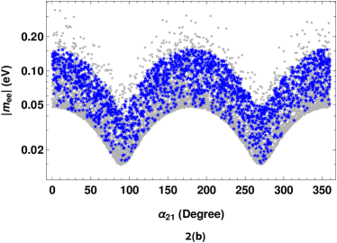
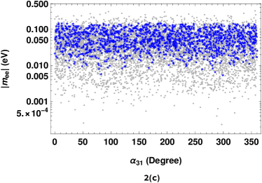
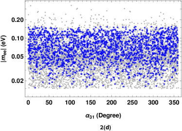
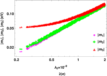
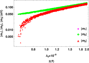
Figure 2: For NH (first column) and IH (second column) of neutrino masses: the grey points show the parameter space that satisfies neutrino oscillation data at $3\sigma$, while the points shown in blue color (“$\filledstar$”) satisfy the simultaneity condition. All the points shown in Figs. 2(e) and 2(f) satisfy the simultaneity condition.

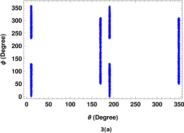
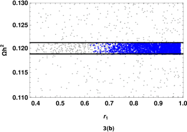
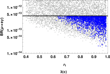
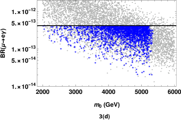
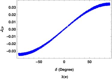
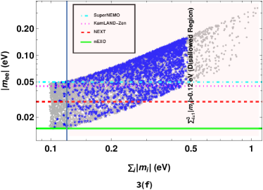
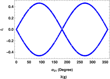
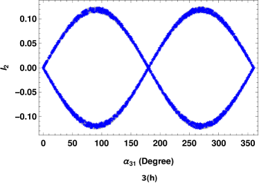
Figure 3: For IH of neutrino masses: the grey points show the parameter space that satisfies neutrino oscillation data at $3\sigma$, while the points shown in blue color (“$\filledstar$”) satisfy the simultaneity condition. The horizontal lines in Fig. 3(b) are experimental range of $\Omega h^{2}$. The horizontal line, in Figs. 3(c) and 3(d), represents experimental upper bound on Br($\mu\rightarrow e\gamma$).

$\lambda_{5}$	$r_{1}$	$r_{3}$	$m_{0}$ $(\text{GeV})$
$1\times 10^{-10}-2\times 10^{-9}$	$0.4-0.99$	$1.1-3.0$	$2000-6000$

Table 1: Ranges for parameters, originating from Scotogenic model, used in the numerical analysis.

5.1 Normal Hierarchy (NH)

For normal hierarchy, we only have one free complex Yukawa coupling, $y_{1}$, which is varied in the range $0\leq|y_{1}|\leq 1.2$. The Majorana phases $\alpha_{2}$ and $\alpha_{3}$ are freely varied using uniform random numbers in the range $0$ to $2\pi$. We have identified benchmark point corresponding to $y_{1}=-0.869-0.144i$, $\alpha_{2}=115.07^{o}$, and $\alpha_{3}=203.8^{o}$, which, simultaneously, satisfy the $3\sigma$ range of the neutrino oscillation data [97] and the experimental constraints on the CDM relic density given by $\Omega h^{2}=0.1200\pm 0.0012$ [104], as well as the upper bound on the LFV branching ratio, Br($\mu\rightarrow e\gamma$)$\leq 4.2\times 10^{-13}$ [98] as shown in third column of Table 2. We refer to this condition of simultaneous satisfaction as the “simultaneity condition”. In Fig. 1, we present correlation plots with two types of points: the grey points represent parameter space that satisfy the neutrino oscillation data at $3\sigma$, while points denoted by ”star”, which are of primary interest, satisfy the simultaneity condition.

The correlation plot between parameters $\theta$ and $\phi$ are shown in Fig. 1(a). It is evident from Fig. 1(a) that there exist two distinct regions of parameter space under simultaneity constraint viz., (i) for $\theta\backsimeq 10^{o}\text{ or }190^{o}$: $\phi\in(0^{o}-130^{o})\oplus(230^{o}-360^{o})$ (ii) for $\theta\backsimeq 170^{o}\text{ or }350^{o}$: $\phi\in(50^{o}-310^{o})$. It can be observed from Figs. 1(b) and 1(c) that higher values of $r_{1}$ are more preferred to satisfy the simultaneity condition. Since $r_{1}$ is the ratio of $M_{1}$ to $m_{0}$, this suggests that having these masses closer to each other increases the likelihood of satisfying both bounds. Additionally, higher values of $r_{1}$ can lead to smaller values of the LFV branching ratio Br($\mu\rightarrow e\gamma$), of the order of $\mathcal{O}(10^{-17})$. In Fig. 1(d), we depict the variation of Br($\mu\rightarrow e\gamma$) with $m_{0}$, which is spread almost uniformly in the range of $m_{0}$ up to $\approx 5300\,\text{GeV}$. Higher values of $m_{0}$ are not preferred to satisfy the simultaneity condition, as evident from the figure. The Jarlskog CP invariant varies between the range of $(-0.036$ to $0.036)$, and the Dirac CP-violating phase $\delta$ varies between $(-90^{o}$ to $90^{o})$ approximately. The blue points are uniformly spread over the entire range of these values, as shown in Fig. 1(e).

The values of the effective Majorana mass $|m_{ee}|$ and the sum of neutrino masses $\sum_{i}|m_{i}|$ are constrained by the simultaneity condition, as depicted in Fig. 1(f). The values allowed by simultaneity condition for $|m_{ee}|$ lie in the range $(0.0055$ to $0.15)$ eV, and for $\sum_{i}|m_{i}|$, values lie in $(0.088$ to $0.49)$ eV range. The shaded region represents the cosmologically disallowed region from Planck data [TT, TE, EE+lowE+lensing+BAO], which imposes a stringent upper bound of $0.12$ eV at $95\%$ confidence level (CL) [104] for the sum of neutrino masses $(\sum_{i=1}^{3}|m_{i}|)$. Different horizontal lines indicate the experimental sensitivity of current and future $0\nu\beta\beta$ decay experiments: SuperNEMO[123], KamLAND-Zen[124], NEXT[125, 126], and nEXO[127]. Considering the cosmological bound on sum of neutrino masses $\sum_{i}|m_{i}|$, the simultaneity condition predicts $|m_{ee}|\in(0.0055-0.03)$ eV range which can be probed at nEXO $0\nu\beta\beta$ decay experiment.

In addition to the Jarlskog CP invariant, the Majorana CP invariants $I_{1}$ and $I_{2}$ are also computed with Majorana phases $\alpha_{21}$ and $\alpha_{31}$, as shown in Figs. 1(g) and 1(h) respectively. For $I_{1}$, the allowed range is $(-0.46\,\,\text{to}\,\,0.46)$, and for $I_{2}$, it is $(-0.12\,\,\text{to}\,\,0.12)$. Both $\alpha_{21}$ and $\alpha_{31}$ vary in the entire range from $0^{o}$ to $360^{o}$.

In Figs. 2(a) and 2(c), we depict the correlation plot of Majorana phases $\alpha_{21}$ and $\alpha_{31}$ with $|m_{ee}|$, respectively. It is evident from Fig. 2(a) that $|m_{ee}|$ attains maximum value when the Majorana CP phase $\alpha_{21}$ is near $0^{o},\,180^{o}\,\text{or}\,360^{o}$, and minimum values around $90^{o}\,\text{or}\,\,270^{o}$. However, there is no sharp correlation visible with $\alpha_{31}$.

In Fig. 2(e), we present the plot of the Higgs quartic coupling $\lambda_{5}$ and three neutrino masses, where each point shown in different colors satisfies the simultaneity condition. The smallest value of the lightest neutrino mass $|m_{1}|$ is $0.016$ eV which corresponds to the smallest obtained value of $\lambda_{5}\,\,(\approx 2\times 10^{-10}$). It can be observed that for smaller values of $\lambda_{5}$, the neutrino masses are also small, but they cannot be too small. As $\lambda_{5}$ increases, neutrino masses, also, increase and tend towards a degenerate region. Fig. 2(e) indicates that higher values of $\lambda_{5}$ are more preferred to satisfy the simultaneity condition than lower ones, as higher side parameter space is densely populated.

5.2 Inverted Hierarchy (IH)

For inverted hierarchy, we have only one free complex Yukawa coupling, $y_{3}$, which is varied in the range $0\leq|y_{3}|\leq 1.2$. The Majorana phases $\alpha_{1}$ and $\alpha_{2}$ are randomly varied using uniform distribution in the range $0$ to $2\pi$. The benchmark point corresponding to $y_{3}=0.060+0.024i$, $\alpha_{1}=342.78^{o}$, and $\alpha_{2}=253.29^{o}$ consistent with the simultaneity condition is shown in fourth column of Table 2.

The similar trend as was observed for NH can, also, be seen here. In Figs. 2(b) and 2(d), the correlation of Majorana CP phases with the effective Majorana mass $|m_{ee}|$ are shown. In Fig. 2(f), it can be observed that the smallest value of the lightest neutrino mass $|m_{3}|$ is $0.0027$ eV, which corresponds to the smallest value of $\lambda_{5}\,\,(\approx 6\times 10^{-10}$). This observation, in comparison to the NH, reveals that IH can have very small mass for the lightest neutrino within a small interval of $\lambda_{5}$ around $\lambda_{5}=6\times 10^{-10}$. However, the heavier masses $|m_{1}|$ and $|m_{2}|$ are very close to each other with value approximately $0.05$ eV, even for the smallest obtained value of $\lambda_{5}$. Consequently, sum of neutrino masses attain higher values. The neutrino masses around this small interval of $\lambda_{5}$ make it possible to have sum of neutrino masses $\sum_{i}|m_{i}|$ below the upper bound from Planck cosmological data on $\sum_{i}|m_{i}|$.

The free parameters $\theta$ and $\phi$ exhibit similar behaviour, as that of NH, with two distinct regions, as evident from Fig. 3(a). For $r_{1}$, higher values are preferred as can be seen from Figs. 3(b) and 3(c). As $r_{1}$ increases, the LFV branching ratio Br($\mu\rightarrow e\gamma$) can be very small, of the order of $\mathcal{O}(10^{-14})$. Similarly, for higher values of $m_{0}$, the LFV branching ratio Br($\mu\rightarrow e\gamma$) can be very small. However, a sharp boundary is observed around $5300\,\text{GeV}$ above which no points satisfy the simultaneity condition, as shown in Fig. 3(d). The Jarlskog CP invariant, as depicted in Fig. 3(e), varies between $(-0.036$ to $0.036)$. The Dirac CP-violating phase $\delta$ varies between $(-90^{o}$ to $90^{o})$.

In this case, the effective Majorana mass $|m_{ee}|$ is constrained to take values from $(0.015$ - $0.15)$ eV, and the sum of neutrino masses $\sum_{i}|m_{i}|$ takes values from $(0.10$ - $0.48)$ eV, as shown in Fig. 3(f). However, taking cosmological bound on sum of neutrino masses $\sum_{i}|m_{i}|$ into consideration, the simultaneity condition predicts $|m_{ee}|\in(0.015-0.05)$ eV range which is well within the sensitivity limits of the $0\nu\beta\beta$ decay experiments. The non-observation of this process shall rule out IH predicted by the model. Furthermore, if the bound coming from cosmological observations on $\sum_{i}|m_{i}|$ becomes more stringent ($\backsimeq 0.1$ eV), the IH shall again be ruled out.

The Majorana CP invariants $I_{1}$ and $I_{2}$, along with their corresponding Majorana phases $\alpha_{21}$ and $\alpha_{31}$, are shown in Figs. 3(g) and 3(h), respectively. The range obtained for $I_{1}$ is $(-0.46$ to $0.46)$ and for $I_{2}$, it is $(-0.12$ to $0.12)$ approximately. The Majorana phases $\alpha_{21}$ and $\alpha_{31}$ vary in the entire range from $0^{o}$ to $360^{o}$.

S.No.	Parameters	NH	IH	NH
				(Extended Magic Symmtery)
1.	$\theta\,(^{o})$	169.68	190.59	169.83
2.	$\phi\,(^{o})$	264.56	242.29	304.37
3.	$\lambda_{5}$	3.10$\times$ 10-10	6.28$\times$ 10-10	3.34$\times$ 10-10
4.	$r_{1}$	0.90	0.96	0.96
5.	$r_{3}$	2.10	1.74	1.70
6.	$m_{0}$ $(\text{GeV})$	2978	4829	3229
7.	$\Delta m^{2}_{21}\,(\text{eV}^{2})$	7.18$\times$10-5	7.08$\times$10-5	8.07$\times$10-5
8.	$\Delta m^{2}_{31}\,(\text{eV}^{2})$	2.49$\times$10-3	2.45$\times$10-3	2.49$\times$10-3
9.	$\theta_{13}\,(^{o})$	8.14	8.63	8.29
10.	$\theta_{12}\,(^{o})$	35.7	35.7	35.7
11.	$\theta_{23}\,(^{o})$	45.56	42.15	41.68
12.	$\Omega h^{2}$	0.120	0.120	0.120
13.	$Br(\mu\rightarrow e\gamma)$	9.48$\times$10-14	3.85$\times$10-13	6.51$\times$10-14

Table 2: Benchmark points consistent with simultaneity condition i.e. satisfying neutrino oscillation data at $3\sigma$, experimental bounds on $\Omega h^{2}$ and Br($\mu\rightarrow e\gamma$). The point shown in last column, also, satisfy the extended magic symmetry.

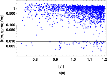
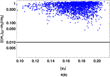
Figure 4: The points that satisfy simultaneity condition shown on left side for NH and on right side for IH, where points on and below the black horizontal line (which represents the tolerance) satisfy the extended magic symmetry constraint.

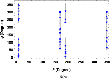
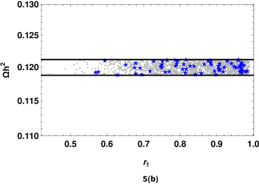
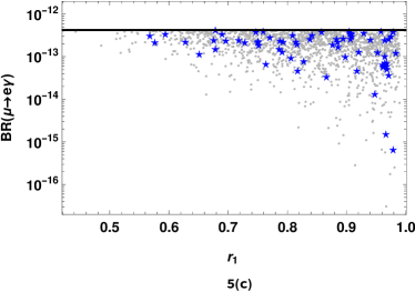
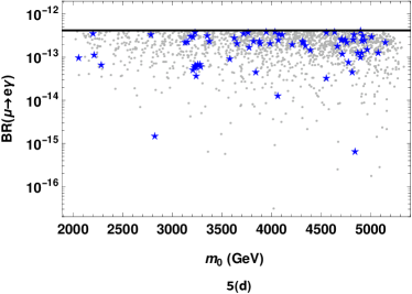
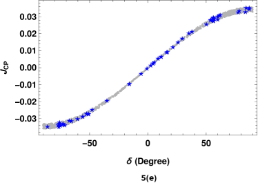
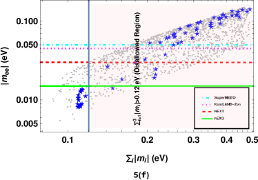
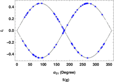
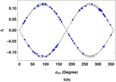
Figure 5: For NH of neutrino masses: the grey points show the parameter space that satisfies simultaneity condition, while the points shown in blue color (“$\filledstar$”), also, satisfy extended magic condition. The horizontal lines in Fig. 5(b) are experimental range of $\Omega h^{2}$. The horizontal line, in Figs. 5(c) and 5(d), represents experimental upper bound on Br($\mu\rightarrow e\gamma$).

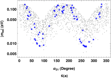
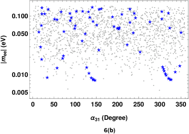
Figure 6: For NH of neutrino masses: the grey points show the parameter space that satisfies simultaneity condition, while the points shown in blue color (“$\filledstar$”), also, satisfy extended magic condition. In Fig. 6(c) the points represented by “$\bullet$”, “$\blacklozenge$”, and “$\blacktriangle$” symbols satisfy simultaneity condition as well as extended magic symmetry.

6 Extended Magic Symmetry

Hitherto, we have adopted the trimaximal (TM₂) structure for the neutrino mixing matrix together with the constraints originating from the diagonalization condition of the neutrino mass matrix $m_{\nu}$. This adoption allows us to parameterize the Yukawa coupling matrix $y$ in terms of three independent Yukawa couplings: $y_{1}$, $y_{2}$, and $y_{3}$. Utilizing this parameterized Yukawa coupling matrix $y$, we derive the neutrino mass matrix $m_{\nu}$. Due to the TM₂ mixing scheme, $m_{\nu}$ is a magic matrix with a magic sum equal to $m_{2}$ (see Eqn. (49)). The TM₂ matrix diagonalizes $m_{\nu}$, yielding the neutrino masses $m_{1}$, $m_{2}$, and $m_{3}$ which depends on Yukawa couplings $y_{1}$, $y_{2}$, and $y_{3}$ respectively (see Eqn. (36)). To be phenomenologically viable, these masses must satisfy the mass-squared differences, which further reduces the number of independent Yukawa coupling parameters to one, $y_{1}$ ($y_{3}$) for NH (IH). Using the resulting matrix $m_{\nu}$, we investigate neutrino phenomenology, relic density of DM and possible LFV in $\mu\rightarrow e\gamma$ process.

As mentioned earlier, it is possible to assume certain structures or patterns in $m_{\nu}$, which can allow us to completely determine the remaining Yukawa coupling $y_{1}$ ($y_{3}$). Building on our previous work[83], wherein we have proposed an ansatze for $m_{\nu}$ with an extended magic symmetry, we explore its impact on prediction of the model discussed in Section 5.

Extended Magic Symmetry: Under this extension of the TM₂ mixing scenario, (2,2) element of the neutrino mass matrix is equal to the magic sum i.e. $m_{2}$. The symmetry origin of this mass relation has been presented in Ref. [83] with $\Delta(54)$ discrete flavor symmetry.

So, we have $(m_{\nu})_{22}$ element of the neutrino mass matrix (see Eqn. (49) ) equal to the magic sum $m_{2}$ which in the present model translates to the following form:

$$a_{1}^{2}y_{1}^{2}\Lambda_{1}+y_{2}^{2}\Lambda_{2}+a_{3}^{2}y_{3}^{2}\Lambda_{3} = c_{2}y_{2}^{2}\Lambda_{2},$$

$$a_{1}^{2}y_{1}^{2}\Lambda_{1}+y_{2}^{2}\Lambda_{2}+a_{3}^{2}y_{3}^{2}\Lambda_{3}-c_{2}y_{2}^{2}\Lambda_{2} = 0.$$ (54)

For NH, using Eqns. (43) and (44), we can rewrite the above equation as

$$\begin{split}a_{1}^{2}y_{1}^{2}\Lambda_{1}+\frac{1}{|c_{2}|}\sqrt{\Delta m^{2}_{21}+|c_{1}y_{1}^{2}\Lambda_{1}|^{2}}e^{2i\alpha_{2}}+a_{3}^{2}\frac{1}{|c_{3}|}\sqrt{\Delta m^{2}_{31}+|c_{1}y_{1}^{2}\Lambda_{1}|^{2}}e^{2i\alpha_{3}}-\sqrt{\Delta m^{2}_{21}+|c_{1}y_{1}^{2}\Lambda_{1}|^{2}}e^{2i\alpha_{2}}=0.\end{split}$$ (55)

and, for IH, using Eqns. (47) and (48), we have

$$\begin{split}a_{1}^{2}\frac{1}{|c_{1}|}\sqrt{\Delta m^{2}_{31}+|c_{3}y_{3}^{2}\Lambda_{3}|^{2}}e^{2i\alpha_{1}}&+\frac{1}{|c_{2}|}\sqrt{\Delta m^{2}_{21}+\Delta m^{2}_{31}+|c_{3}y_{3}^{2}\Lambda_{3}|^{2}}e^{2i\alpha_{2}}+a_{3}^{2}y^{2}_{3}\Lambda_{3}\\ &-\sqrt{\Delta m^{2}_{21}+\Delta m^{2}_{31}+|c_{3}y_{3}^{2}\Lambda_{3}|^{2}}e^{2i\alpha_{2}}=0.\end{split}$$ (56)

We can see from these equations that $y_{1}$ becomes a function of $\lambda_{5}$, $r_{1}$, and $m_{0}$ (through $\Lambda_{1}$), while $y_{3}$ becomes a function of $\lambda_{5}$, $r_{3}$, and $m_{0}$ (through $\Lambda_{3}$). Both depend on the free parameters $\theta$ (through $a_{1}$, $a_{3}$, $c_{1}$, and $c_{3}$) and $\phi$ (through $a_{1}$ and $a_{3}$). Also, dependence of $y_{1}$ ($y_{3}$) on phases $\alpha_{2}$ and $\alpha_{3}$ ( $\alpha_{1}$ and $\alpha_{2}$) is clearly visible. In this case, $y_{1}$ and $y_{3}$ are not free anymore; they have to satisfy constraints originating from extended magic symmetry.

6.1 Numerical Analysis and Discussion

In this section, we vary the neutrino mass-squared differences, $\theta$, $\phi$, and the parameters of the Scotogenic model within the same range as mentioned in the previous section. Yukawa couplings $y_{1}$ and $y_{3}$ are not free parameters anymore but are solutions to Eqns. (55) and (56), respectively. We solve these equations numerically considering those values of the Yukawa couplings as solutions for which $\left|\frac{(m_{\nu})_{22}-m_{2}}{m_{2}}\right|\leq 10^{-2}$ and $0\leq|y_{1}|,|y_{3}|\leq 1.2$. Furthermore, we vary $\alpha_{2}$ and $\alpha_{3}$ in NH ($\alpha_{1}$ and $\alpha_{2}$ in IH), randomly in the range from $0$ to $2\pi$, with uniform distribution.

6.2 Normal Hierarchy

We have obtained the benchmark point corresponding to $y_{1}=0.909-0.163i$, $\alpha_{2}=248.12^{o}$ and $\alpha_{3}=128.74^{o}$ which satisfy the simultaneity condition along with the extended magic condition, as shown in fifth column of Table 2. The correlation plot illustrating the relation between $\left|\frac{(m_{\nu})_{22}-m_{2}}{m_{2}}\right|$ and the Yukawa coupling strength $|y_{1}|$ is depicted in Fig. 4(a). The black horizontal line represents the tolerance of $10^{-2}$, where any point on or below this line corresponds to a solution to Eqn. (55). The results obtained are displayed in Fig. 5. Since we are imposing two conditions, namely the simultaneity condition and the extended magic symmetry, it is expected that some of the regions or points allowed by the simultaneity condition alone will be filtered out by the extended magic condition. Consequently, the number of points obtained is considerably fewer compared to when only one condition is imposed. As observed in correlation plots shown in Fig. 5, the trend is quite similar to NH without extended magic symmetry.

The values of the effective Majorana mass $|m_{ee}|$ and the sum of neutrino masses $\sum_{i}|m_{i}|$ are constrained by both conditions, as depicted in Fig. 5(f). The allowed points are now constrained within a very small region, as most of the part is disallowed by cosmological data for the sum of neutrino masses. These values of $|m_{ee}|$ lie beyond the sensitivity of the current and future $0\nu\beta\beta$ decay experiments. Figs. 6(a) and 6(b) depict the correlation plots of $\alpha_{21}$ and $\alpha_{31}$ with $|m_{ee}|$, respectively. In Fig. 6(c), the plot showcases the relationship between the Higgs quartic coupling $\lambda_{5}$ and three neutrino masses, where each point, represented by different colors, satisfies the simultaneity condition and the extended magic condition. It is to be noted that extended magic symmetry scenario prefers higher values of $\lambda_{5}$ as compared to the only TM₂ scenario discussed in section 5.

6.3 Inverted Hierarchy

As depicted in Fig. 4(b), there are no points below the tolerance level. This observation is remarkable as it indicates that if both these conditions (simultaneity and extended magic conditions) need to be fulfilled simultaneously, then IH is ruled out.

7 Conclusions

We have studied the Scotogenic model where we have used matrix $U_{\text{TM}_{2}}$ as the neutrino mixing matrix, and using the diagonalization condition for the flavor neutrino mass matrix $m_{\nu}$, we have parameterized the Yukawa coupling matrix $y$. We have investigated the allowed parameter space of the model satisfying experimental bounds on relic density of CDM and possible LFV alongside neutrino oscillation data, which we called the simultaneity condition, in the framework of trimaximal mixing paradigm. In particular, we have studied two scenarios: (i) wherein $m_{\nu}$ is magic symmetric, and (ii) $m_{\nu}$ has extended magic symmetry i.e., $(m_{\nu})_{22}$ element of $m_{\nu}$ is, also, equal to the magic sum $m_{2}$.

In first scenario, both normal as well as inverted hierarchies of neutrino mass are allowed by the simultaneity condition. For the free parameters $\theta$ and $\phi$ there exist two distinct regions of parameter space under simultaneity constraint viz., (i) for $\theta\backsimeq 10^{o}\text{ or }190^{o}$: $\phi\in(0^{o}-130^{o})\oplus(230^{o}-360^{o})$ (ii) for $\theta\backsimeq 170^{o}\text{ or }350^{o}$: $\phi\in(50^{o}-310^{o})$ in both hierarchies. Also in both hierarchies, the Dirac phase $\delta$ and Majorana phases $\alpha_{21}$, $\alpha_{31}$ span the entire allowed range, with the Jarlskog invariant $J_{CP}$ varying in the range $(-0.036$ to $0.036)$ and the Majorana CP invariants $I_{1}$ and $I_{2}$ varying in the range $(-0.46$ to $0.46)$ and $(-0.12$ to $0.12)$, respectively. The effective Majorana mass $|m_{ee}|$ takes the range $(0.0055$ to $0.15)\,\text{eV}$ for NH and $(0.015$ to $0.15)\,\text{eV}$ for IH. However, a significant region of $|m_{ee}|$ is excluded by the cosmological bound on the sum of neutrino masses. Considering the cosmological bound on sum of neutrino masses $\sum_{i}|m_{i}|$, the simultaneity condition predicts $|m_{ee}|\in(0.0055-0.03)$ eV range for NH and $|m_{ee}|\in(0.015-0.05)$ eV range for IH. The predicted range of $|m_{ee}|$ can be probed at $0\nu\beta\beta$ decay experiments which is well within the sensitivity limits of the $0\nu\beta\beta$ decay experiments for IH. If this process is not observed, it will rule out the IH predicted by the model. Furthermore, if the upper limit derived from cosmological observations on the sum of neutrino masses ($\sum_{i}|m_{i}|$) becomes more restrictive ($\backsimeq 0.1$ eV), the inverted hierarchy will again be excluded.

In second scenario, IH is disallowed (Fig. 4(b)), and for NH, the obtained parameter space resembles with that of first scenario. However, the range of $|m_{ee}|$ obtained in second scenario, consistent with the cosmological bound on the sum of neutrino masses, is highly constrained. The more stringent bounds coming from cosmological data on the sum of neutrino masses in the future can test the viability of NH with extended magic symmetry.

For NH, the obtained values of neutrino masses for the second scenario take higher values which corresponds to the higher value of quartic coupling, $\lambda_{5}$. In turn, this pushes the sum of neutrino masses to go up and hence in second scenario we have more tight constraint from cosmological data on the sum of neutrino masses.

In summary, our investigation sheds light on the interplay between the Scotogenic model and TM₂ mixing leading to the reduction in the number of free parameters and stringent constraints on the allowed parameter space. Our model is predicting NH of neutrino masses with both CP conserving and CP violating solutions along with exclusion of the inverted hierarchy in presence of the extended magic symmetry.

Acknowledgments
Tapender acknowledges the financial support provided by Central University of Himachal Pradesh. The authors, also, acknowledge Department of Physics and Astronomical Science for providing necessary facility to carry out this work.

References

- [1] E. Ma, Phys. Rev. D 73, 077301 (2006).
- [2] E. Ma and D. Suematsu, Mod. Phys. Lett. A 24, 583-589 (2009).
- [3] Y. Farzan, Phys. Rev. D 80, 073009 (2009).
- [4] Y. Farzan, S. Pascoli and M. A. Schmidt, JHEP 10, 111 (2010).
- [5] D. Hehn and A. Ibarra, Phys. Lett. B 718, 988-991 (2013).
- [6] V. Brdar, I. Picek and B. Radovcic, Phys. Lett. B 728, 198-201 (2014).
- [7] W. Chao, Int. J. Mod. Phys. A 30, no.01, 1550007 (2015).
- [8] F. von der Pahlen, G. Palacio, D. Restrepo and O. Zapata, Phys. Rev. D 94, no.3, 033005 (2016).
- [9] P. Rocha-Moran and A. Vicente, JHEP 07, 078 (2016).
- [10] A. Ibarra, C. E. Yaguna and O. Zapata, Phys. Rev. D 93, no.3, 035012 (2016).
- [11] P. M. Ferreira, W. Grimus, D. Jurciukonis and L. Lavoura, JHEP 07, 010 (2016).
- [12] W. B. Lu and P. H. Gu, Nucl. Phys. B 924, 279-311 (2017).
- [13] D. Mahanta and D. Borah, JCAP 11, 021 (2019).
- [14] D. Borah, P. S. B. Dev and A. Kumar, Phys. Rev. D 99, no.5, 055012 (2019).
- [15] E. C. F. S. Fortes, A. C. B. Machado, J. Montaño and V. Pleitez, Phys. Lett. B 803, 135289 (2020).
- [16] D. Borah, M. Dutta, S. Mahapatra and N. Sahu, Phys. Rev. D 105, no.1, 015029 (2022).
- [17] L. Singh, D. Mahanta and S. Verma, [arXiv:2309.12755 [hep-ph]].
- [18] P. F. Harrison, D. H. Perkins and W. G. Scott, Phys. Lett. B 458, 79-92 (1999).
- [19] P. F. Harrison, D. H. Perkins and W. G. Scott, Phys. Lett. B 530, 167 (2002).
- [20] Z. z. Xing, Phys. Lett. B 533, 85-93 (2002).
- [21] P. F. Harrison and W. G. Scott, Phys. Lett. B 535, 163-169 (2002).
- [22] P. F. Harrison and W. G. Scott, Phys. Lett. B 557, 76 (2003).
- [23] X. G. He and A. Zee, Phys. Lett. B 560, 87-90 (2003).
- [24] N. Li and B. Q. Ma, Phys. Rev. D 71, 017302 (2005).
- [25] Z. Z. Xing, Chin. Phys. C 36, 101-105 (2012).
- [26] S. Zhou, Phys. Lett. B 704, 291-295 (2011).
- [27] T. Araki, Phys. Rev. D 84, 037301 (2011).
- [28] N. Haba and R. Takahashi, Phys. Lett. B 702, 388-393 (2011).
- [29] W. Chao and Y. j. Zheng, JHEP 02, 044 (2013).
- [30] H. Zhang and S. Zhou, Phys. Lett. B 704, 296-302 (2011).
- [31] W. Rodejohann, H. Zhang and S. Zhou, Nucl. Phys. B 855, 592-607 (2012).
- [32] D. Marzocca, S. T. Petcov, A. Romanino and M. Spinrath, JHEP 11, 009 (2011).
- [33] S. Antusch, S. F. King, C. Luhn and M. Spinrath, Nucl. Phys. B 856, 328-341 (2012).
- [34] S. Dev, S. Gupta and R. Raman Gautam, Phys. Lett. B 704, 527-533 (2011).
- [35] S. F. Ge, D. A. Dicus and W. W. Repko, Phys. Rev. Lett. 108, 041801 (2012).
- [36] S. F. Ge, D. A. Dicus and W. W. Repko, Phys. Lett. B 702, 220-223 (2011).
- [37] P. O. Ludl, S. Morisi and E. Peinado, Nucl. Phys. B 857, 411-423 (2012).
- [38] A. S. Joshipura and K. M. Patel, JHEP 09, 137 (2011).
- [39] S. Morisi, K. M. Patel and E. Peinado, Phys. Rev. D 84, 053002 (2011).
- [40] P. S. Bhupal Dev, R. N. Mohapatra and M. Severson, Phys. Rev. D 84, 053005 (2011).
- [41] R. de Adelhart Toorop, F. Feruglio and C. Hagedorn, Phys. Lett. B 703, 447-451 (2011).
- [42] A. Adulpravitchai and R. Takahashi, JHEP 09, 127 (2011).
- [43] Q. H. Cao, S. Khalil, E. Ma and H. Okada, Phys. Rev. D 84, 071302 (2011).
- [44] T. Araki and C. Q. Geng, JHEP 09, 139 (2011).
- [45] A. Rashed, Nucl. Phys. B 874, 679-697 (2013).
- [46] A. Rashed and A. Datta, Phys. Rev. D 85, 035019 (2012).
- [47] A. Aranda, C. Bonilla and A. D. Rojas, Phys. Rev. D 85, 036004 (2012).
- [48] D. Meloni, JHEP 02, 090 (2012).
- [49] S. F. King and C. Luhn, JHEP 03, 036 (2012).
- [50] M. Kashav and S. Verma, Int. J. Theor. Phys. 62, no.12, 267 (2023).
- [51] Z. h. Zhao, JHEP 09, 023 (2017).
- [52] K. S. Channey and S. Kumar, J. Phys. G 48, no.3, 035003 (2021).
- [53] N. Haba, A. Watanabe and K. Yoshioka, Phys. Rev. Lett. 97, 041601 (2006).
- [54] X. G. He and A. Zee, Phys. Lett. B 645, 427-431 (2007).
- [55] W. Grimus and L. Lavoura, JHEP 09, 106 (2008).
- [56] H. Ishimori, Y. Shimizu, M. Tanimoto and A. Watanabe, Phys. Rev. D 83, 033004 (2011).
- [57] Y. Shimizu, M. Tanimoto and A. Watanabe, Prog. Theor. Phys. 126, 81-90 (2011).
- [58] X. G. He and A. Zee, Phys. Rev. D 84, 053004 (2011).
- [59] I. de Medeiros Varzielas and D. Pidt, JHEP 03, 065 (2013).
- [60] Z. H. Zhao, X. Zhang, S. S. Jiang and C. X. Yue, Int. J. Mod. Phys. A 35, no.07, 2050039 (2020).
- [61] S. F. King and Y. L. Zhou, Phys. Rev. D 101, no.1, 015001 (2020).
- [62] P. P. Novichkov, S. T. Petcov and M. Tanimoto, Phys. Lett. B 793, 247-258 (2019).
- [63] W. Rodejohann and X. J. Xu, Phys. Rev. D 96, no.5, 055039 (2017).
- [64] C. Luhn, Nucl. Phys. B 875, 80-100 (2013).
- [65] S. F. King and C. Luhn, JHEP 09, 042 (2011).
- [66] S. Kumar, Phys. Rev. D 82, 013010 (2010) [erratum: Phys. Rev. D 85, 079904 (2012)].
- [67] S. Dev and D. Raj, Adv. High Energy Phys. 2022, 4952562 (2022).
- [68] W. Grimus, L. Lavoura and A. Singraber, Phys. Lett. B 686, 141-145 (2010).
- [69] C. H. Albright and W. Rodejohann, Eur. Phys. J. C 62, 599-608 (2009).
- [70] Z. h. Zhao, X. Y. Zhao and H. C. Bao, Phys. Rev. D 105, no.3, 035011 (2022).
- [71] G. J. Ding, J. N. Lu and J. W. F. Valle, Phys. Lett. B 815, 136122 (2021).
- [72] W. Rodejohann and H. Zhang, Phys. Rev. D 86, 093008 (2012).
- [73] H. Zhang and Y. L. Zhou, [arXiv:2401.17810 [hep-ph]].
- [74] J. Ganguly, J. Gluza, B. Karmakar and S. Mahapatra, [arXiv:2311.15997 [hep-ph]].
- [75] Y. Chen, Y. Hyodo and T. Kitabayashi, [arXiv:2306.13243 [hep-ph]].
- [76] R. R. Gautam and S. Kumar, Phys. Rev. D 94, no.3, 036004 (2016) [erratum: Phys. Rev. D 100, no.3, 039902 (2019)].
- [77] S. Kumar and R. R. Gautam, Phys. Rev. D 96, no.1, 015020 (2017).
- [78] G. J. Ding, S. F. King and A. J. Stuart, JHEP 12, 006 (2013).
- [79] M. A. Loualidi, [arXiv:2104.13734 [hep-ph]].
- [80] R. R. Gautam, Phys. Rev. D 97, no.5, 055022 (2018).
- [81] S. Kumar and R. R. Gautam, [arXiv:2312.07150 [hep-ph]].
- [82] I. A. Mazumder and R. Dutta, [arXiv:2309.04394 [hep-ph]].
- [83] L. Singh, Tapender, M. Kashav and S. Verma, EPL 142, no.6, 64002 (2023).
- [84] K. S. Channey and S. Kumar, J. Phys. G 46, no.1, 015001 (2019).
- [85] M. J. S. Yang, PTEP 2022, no.1, 013B12 (2022).
- [86] J. A. Casas and A. Ibarra, Nucl. Phys. B 618, 171-204 (2001).
- [87] S. Y. Ho and J. Tandean, Phys. Rev. D 87, 095015 (2013).
- [88] S. Y. Ho and J. Tandean, Phys. Rev. D 89, 114025 (2014).
- [89] S. Singirala, Chin. Phys. C 41, no.4, 043102 (2017).
- [90] D. Suematsu, T. Toma and T. Yoshida, Phys. Rev. D 79, 093004 (2009).
- [91] D. Suematsu, T. Toma and T. Yoshida, Phys. Rev. D 82, 013012 (2010).
- [92] T. Kitabayashi, Phys. Rev. D 98, no.8, 083011 (2018).
- [93] T. Kitabayashi, Int. J. Mod. Phys. A 34, no.19, 1950098 (2019).
- [94] Ankush, M. Kashav, S. Verma and B. C. Chauhan, Phys. Lett. B 824, 136796 (2022).
- [95] T. Kitabayashi, S. Ohkawa and M. Yasuè, Int. J. Mod. Phys. A 32, no.32, 1750186 (2017).
- [96] Ankush, R. Verma, S. Kumar and B. C. Chauhan, JCAP 08, 062 (2023).
- [97] P. F. de Salas, D. V. Forero, S. Gariazzo, P. Martínez-Miravé, O. Mena, C. A. Ternes, M. Tórtola and J. W. F. Valle, JHEP 02, 071 (2021).
- [98] A. M. Baldini et al. [MEG], Eur. Phys. J. C 76, no.8, 434 (2016).
- [99] W. H. Bertl et al. [SINDRUM II], Eur. Phys. J. C 47, 337-346 (2006).
- [100] B. Aubert et al. [BaBar], Phys. Rev. Lett. 104, 021802 (2010).
- [101] K. Hayasaka, K. Inami, Y. Miyazaki, K. Arinstein, V. Aulchenko, T. Aushev, A. M. Bakich, A. Bay, K. Belous and V. Bhardwaj, et al. Phys. Lett. B 687, 139-143 (2010).
- [102] U. Bellgardt et al. [SINDRUM], Nucl. Phys. B 299, 1-6 (1988).
- [103] C. Dohmen et al. [SINDRUM II], Phys. Lett. B 317, 631-636 (1993).
- [104] N. Aghanim et al. [Planck], Astron. Astrophys. 641, A6 (2020) [erratum: Astron. Astrophys. 652, C4 (2021)].
- [105] C. S. Lam, Phys. Lett. B 640, 260-262 (2006).
- [106] P. F. Harrison and W. G. Scott, Phys. Lett. B 594, 324-332 (2004).
- [107] R. Friedberg and T. D. Lee, HEPNP 30, 591-598 (2006).
- [108] S. Verma and M. Kashav, J. Phys. G 47, no.8, 085003 (2020).
- [109] Y. Hyodo and T. Kitabayashi, Chin. Phys. C 47, no.4, 043103 (2023).
- [110] Y. Hyodo and T. Kitabayashi, PTEP 2021, no.12, 123B08 (2021).
- [111] Y. Hyodo and T. Kitabayashi, Int. J. Mod. Phys. A 35, no.29, 2050183 (2020).
- [112] R. Minamizawa, Y. Hyodo and T. Kitabayashi, Int. J. Mod. Phys. A 37, no.31n32, 2250191 (2022).
- [113] J. Kubo, E. Ma and D. Suematsu, Phys. Lett. B 642, 18-23 (2006).
- [114] K. Griest and D. Seckel, Phys. Rev. D 43, 3191-3203 (1991).
- [115] T. Toma and A. Vicente, JHEP 01, 160 (2014).
- [116] C. Jarlskog, Phys. Rev. Lett. 55, 1039 (1985).
- [117] S. M. Bilenky and S. T. Petcov, Rev. Mod. Phys. 59, 671 (1987) [erratum: Rev. Mod. Phys. 61, 169 (1989); erratum: Rev. Mod. Phys. 60, 575-575 (1988)].
- [118] P. I. Krastev and S. T. Petcov, Phys. Lett. B 205, 84-92 (1988).
- [119] J. F. Nieves and P. B. Pal, Phys. Rev. D 36, 315 (1987).
- [120] J. A. Aguilar-Saavedra and G. C. Branco, Phys. Rev. D 62, 096009 (2000).
- [121] S. M. Bilenky, S. Pascoli and S. T. Petcov, Phys. Rev. D 64, 053010 (2001).
- [122] J. F. Nieves and P. B. Pal, Phys. Rev. D 64, 076005 (2001).
- [123] A. S. Barabash, J. Phys. Conf. Ser. 375, 042012 (2012).
- [124] A. Gando et al. [KamLAND-Zen], Phys. Rev. Lett. 117, no.8, 082503 (2016).
- [125] F. Granena et al. [NEXT], [arXiv:0907.4054 [hep-ex]].
- [126] J. J. Gomez-Cadenas et al. [NEXT], Adv. High Energy Phys. 2014, 907067 (2014).
- [127] C. Licciardi [nEXO], J. Phys. Conf. Ser. 888, no.1, 012237 (2017).