Using Spherical Harmonics to solve the Boltzmann equation: an operator based approach

Abstract

The transport of charged particles or photons in a scattering medium can be modelled with a Boltzmann equation. The mathematical treatment for scattering in such scenarios is often simplified if evaluated in a frame where the scattering centres are, on average, at rest. It is common therefore, to use a mixed coordinate system, wherein space and time are measured in a fixed inertial frame, while momenta are measured in a “co-moving” frame. To facilitate analytic and numerical solutions, the momentum dependency of the phase-space density may be expanded as a series of spherical harmonics, typically truncated at low order. A method for deriving the system of equations for the expansion coefficients of the spherical harmonics to arbitrary order is presented in the limit of isotropic, small-angle scattering. The method of derivation takes advantage of operators acting on the space of spherical harmonics. The matrix representations of these operators are employed to compute the system of equations. The computation of matrix representations is detailed and subsequently simplified with the aid of rotations of the coordinate system. The eigenvalues and eigenvectors of the matrix representations are investigated to prepare the application of standard numerical techniques, e.g. the finite volume method or the discontinuous Galerkin method, to solve the system.

1 Introduction

The transport of charged particles, photons or neutrinos in an inhomogeneous scattering medium is a recurring problem that appears across multiple sub-fields of physics (e.g. Braginskii, 1958; Chandrasekhar, 1960; Ginzburg & Syrovatskii, 1964; Mihalas & Mihalas, 1984; Lewis & Miller, 1984). Astrophysical contexts include neutrino and radiation hydrodynamics in supernova explosions, as well as the propagation and acceleration of energetic charged particles (cosmic rays). Typically, one considers the evolution of the single particle phase-space density, $f(\textbf{{x}},\textbf{{p}},t)$ by solving a transport equation which can be written in the form $\frac{\textrm{d}f}{\textrm{d}s}=\hat{C}f\,$. Here $s$ is an affine parameter that defines a point on a photon or particle trajectory (for a photon or neutrino the distance along a ray, for a particle with mass the proper time) and $\hat{C}$ is a collision operator that describes stochastic disturbances of these trajectories. For photons and neutrinos, the trajectories are simply geodesics in the local space-time, and $\hat{C}$ contains the scattering, absorption and emission cross-sections. These may be prescribed in the scattering-centres’ rest frame, which may be determined by solving a separate set of equations (e.g., those of hydro- or magnetohydrodynamics). These equations in turn can be augmented by terms containing moments of $f$, i.e. feedback. In general, the rest frame of the scattering centres is non-inertial, and this must be taken into account when formulating the relevant transport equation (e.g. Achterberg & Norman, 2018).

For example, the phase-function for photon scattering is usually specified in terms of the coordinates of the momenta p and $\textbf{{p}}^{\prime}$ of the photons involved, measured in the “co-moving” frame in which the scattering centres are locally at rest. This leads to a formulation of the radiation transport equation in so-called “mixed” coordinates (Lindquist, 1966; Castor, 1972; Riffert, 1986), with the phase-space density treated as a function of position x and time $t$, both measured in the laboratory frame, while the momentum p, is measured in the co-moving frame.

For cosmic rays, the situation is more complicated. As in the case of photons and neutrinos, one conventionally assumes the presence of a “background” plasma whose evolution can be determined, for example via the equations of ideal magnetohydrodynamics. But, in this case, these are augmented not only by terms in the stress-energy tensor, but also by the current and charge density carried by the cosmic rays. The charged particle trajectories are then not geodesics, but are determined by the electromagnetic fields carried by the background plasma. In dense plasmas, where Coulomb collisions among the different charged species occur, $\hat{C}$ can be modelled in the co-moving frame as a Fokker-Planck operator (Rosenbluth et al., 1957; Shkarofsky et al., 1966). However, in dilute, astrophysical plasmas, Coulomb collisions are unimportant, and $\hat{C}$ is instead used to model the effects of scattering on stochastic turbulent fluctuations that are superimposed on the large-scale fields carried by the background plasma. Given suitable constraints on the properties of this turbulence, $\hat{C}$ can again be formulated as a Fokker-Planck operator, this time in the (non-inertial) wave-frame (e.g. Skilling, 1975; Webb, 1985; Kirk et al., 1988). In principle, the large scale fields take into account the current and charge density of the cosmic rays. Consequently, the left-hand-side of the transport equation resembles a Vlasov equation, which has given rise to the name “Vlasov–Fokker–Planck equation”.

For both photons and charged particles, the single particle phase-space density is a function of six independent variables and time, making direct discretisation approaches prohibitive. In the case of the space and time variables, numerical techniques for solving the MHD equations are well-known. These can be applied also to the VFP equation, since $f$ is not expected to vary on scales shorter or faster than those of the MHD variables. Also, CR distributions are generally smooth functions of the particle energy (or the modulus $p$ of the momentum), so that discretization of this variable is not problematic. However, the two remaining angular variables (in momentum space) pose a problem, since strong anisotropies can develop, in particular close to oblique shock fronts in the background plasma or in the presence of highly relativistic flows. An effective approach here is to expand the phase-space density in a series of known functions, and thereby resolve the anisotropy by extending the expansion to higher order until convergence is achieved (Kirk & Schneider, 1987; Kirk et al., 2023). In the case of cosmic rays in non-relativistic flows, a suitable set of functions is that of spherical harmonics. This is the approach we adopt here, by expanding the single particle distribution in a series of spherical harmonics $Y^{m}_{l}$, which are functions of the spherical polar coordinates $\theta$ and $\phi$ of the momentum vector p (defined with axis along $p_{x}$):

$$f(\textbf{{x}},p,\theta,\varphi,t)=\sum^{\infty}_{l=0}\sum^{l}_{m=-l}f^{m}_{l}(\textbf{{x}},p,t)Y^{m}_{l}(\theta,\varphi)\,,$$ (1.1)

or, equivalently, using Cartesian tensors (Schween & Reville, 2022). The equivalence is particularly well exploited in the (projected-)symmetric trace-free formalism described by Thorne (1980, 1981). Alternatively, it is possible to derive the equations for the moments of the distribution function and, thus, to directly investigate the relevant transport coefficients, see for example Webb (1989) and references therein. Expanding the single particle distribution function reduces the number of dependent variables from six to four, though it requires a procedure to determine an effective transport equation for each coefficient in the expansion. While derivations of this system of equations can be found in the literature for different applications, both for Cartesian expansions (see Johnston, 1960; Williams & Jokipii, 1991; Thomas et al., 2012, truncated at low order) and spherical harmonics (e.g. Bell et al., 2006; Tzoufras et al., 2011; Reville & Bell, 2013), the resulting equations are cumbersome, and the physical meaning is obfuscated.

In this paper we present a simplification of this expansion procedure which avoids lengthy algebraic manipulations, when expanding to high order. This facilitates checking the convergence of the expansion and allows for a direct physical interpretation at each stage. We restrict our derivation to the propagation and acceleration of charged particles in a prescribed background plasma. In Section 2 we introduce the relevant transport equation, namely a variant of the Vlasov–Fokker–Planck (VFP) equation, and simplify it by making the additional, although not necessary, assumption that the co-moving frame moves slowly in the laboratory frame, and that the scattering operator is isotropic. For such a scattering operator, the eigenfunctions are the spherical harmonics used in the expansion. This motivates an approach which exploits operators acting on the space of spherical harmonics and their matrix representations. In Section 3 we identify and define the operators which are present in the VFP equation and show that the system of equations can then be obtained by replacing the operators with their matrix representations. This has the advantage of retaining the original structure of the VFP equation. We explicitly compute the matrix elements of the matrix representations. Moreover, in Section 4 we prove that the effort of computing them can be considerably reduced with the help of rotations of the coordinate system in momentum space. We investigate how these rotations act in the space of spherical harmonics and how they change the operators and their matrix representations. The key insight is that the operators’ matrix representations can be considered as “rotated” versions of each other and thus it is possible to compute any one of them by rotating another. We quote explicit expressions for the necessary rotation matrices. Having derived and simplified the computation of the system of equations, we note that it contains redundant equations. The reason is that the reality of the single particle phase-space density imposes symmetries on the expansion coefficients. In Section 5 we remedy this using the real spherical harmonics. The relation between the complex and real spherical harmonics can be expressed with the help of a basis transformation matrix. Multiplying the system of equations with this basis transformation matrix removes the superfluous equations. Numerically solving the system of equations using standard techniques, e.g. the finite volume method or the discontinuous Galerkin method, requires knowledge about the eigenvalues and eigenvectors of the matrix representations. In the last part of this paper, i.e . in Section 6, we prove that the representation matrices have the same eigenvalues and that there eigenvectors are also rotated versions of each other. Moreover, we show that eigenvalues are the roots of the associated Legendre polynomials. The implementation of the discontinuous Galerkin method exploiting this knowledge is the subject of a companion paper.

2 Particle transport in plasmas

The transport of charged particles and photons in a scattering, non-stationary medium was recently revisited by Achterberg & Norman (2018). Their work provides a rigorous derivation of the mixed-frame transport equation in the context of special relativity. We adopt the mixed-frame transport equation as our starting point, and refer the reader to their paper for further details.

We consider particles that move in a background fluid, whose velocity field can be described with the 4-vector $U^{\mu}=\Gamma(c,\textbf{{U}})$ (bold symbols denoting 3-vectors), with $\Gamma=(1-U^{2}/c^{2})^{-1/2}$ the bulk Lorentz factor of the background fluid. For the particles on the other hand, the four-velocity is $V^{\mu}=\gamma(c,\textbf{{V}})$, with $\gamma=p/mV=\varepsilon/mc^{2}$ the associated particle Lorentz factor. The background plasma is permeated by electric and magnetic fields, E and B. Using unprimed quantities to denote quantities measured in the laboratory frame, and primed quantities to denote those measured in the fluid rest frame, one arrives at the following transport equation

$$\frac{df}{ds}+\left[\gamma^{\prime}q\left(\textbf{{E}}^{\prime}+\textbf{{V}}^{\prime}\times\textbf{{B}}^{\prime}\right)-(\Gamma+1)\varepsilon^{\prime}\frac{d}{ds}\left(\frac{\Gamma\textbf{{U}}}{\Gamma+1}\right)+\textbf{{p}}^{\prime}\times\mn@boldsymbol{\omega}_{\ell}\right]\cdot\nabla_{p^{\prime}}f=\gamma^{\prime}\frac{\nu^{\prime}}{2}\Delta_{\theta^{\prime},\varphi^{\prime}}f\,,$$ (2.1)

where, on account of the mixed coordinates, the proper-time derivative along the particle trajectory is

$$\frac{d\,}{ds}=\frac{\,p^{\nu}}{m}\frac{\partial\,}{\partial x^{\nu}}=\gamma^{\prime}\left\{\Gamma\left(1+\frac{\textbf{{V}}^{\prime}\cdot\textbf{{U}}}{c^{2}}\right)\frac{\partial\,}{\partial t}+\left(\Gamma\textbf{{U}}+\textbf{{V}}^{\prime}\right)\cdot\nabla_{x}+\frac{\Gamma^{2}}{\Gamma+1}\frac{\textbf{{V}}^{\prime}\cdot\textbf{{U}}}{c^{2}}(\textbf{{U}}\cdot\nabla_{x})\right\}\,.$$ (2.2)

As described in Achterberg & Norman (2018, eq. 15), the second two terms inside the square brackets of equation (2.1) correspond to the fictitious forces introduced from the accelerating frame. The $\mn@boldsymbol{\omega}_{\ell}$ vector stems from changes in the direction of U,

$$\mn@boldsymbol{\omega}_{\ell}=(\Gamma-1)\left(\bm{\hat{\ell}}\times\frac{\mathrm{d}\bm{\hat{\ell}}}{\mathrm{d}s}\right)\quad\text{with }\bm{\hat{\ell}}\text{ a unit vector along }\textbf{{U}}=U\bm{\hat{\ell}}\,.$$

The particular form of the collision term we adopt here corresponds to isotropic scattering in the local fluid frame with rate $\nu^{\prime}(p^{\prime})$, although such a simplification is not essential. The symbol $\Delta_{\theta^{\prime},\varphi^{\prime}}$ denotes the Laplace operator in spherical angles,

$$\Delta_{\theta^{\prime},\varphi^{\prime}}=\left(\frac{\partial^{2}}{\partial\theta^{\prime 2}}+\frac{\cos\theta^{\prime}}{\sin\theta^{\prime}}\frac{\partial}{\partial\theta^{\prime}}+\frac{1}{\sin^{2}\theta^{\prime}}\frac{\partial^{2}}{\partial\varphi^{\prime 2}}\right)\,.$$ (2.3)

The collision term thus assumes that the scattering is elastic, changing only the direction of a particle’s momentum and not its magnitude which need not be the case if the scattering centres are dispersive, or anisotropic (Melrose, 1969; Skilling, 1975). A detailed study of these effects is beyond the scope of the current paper.

For $U\ll c$, we can expand equation (2.1) retaining all terms to first order in $U/c$:

$$\left(1+\frac{\textbf{{V}}^{\prime}\cdot\textbf{{U}}}{c^{2}}\right)\frac{\partial f}{\partial t}+\left(\textbf{{U}}+\textbf{{V}}^{\prime}\right)\cdot\nabla_{x}f+\left[\left(q\textbf{{E}}^{\prime}-\gamma^{\prime}m\frac{\mathrm{d}\textbf{{U}}}{\mathrm{d}t}\right)-(\textbf{{p}}^{\prime}\cdot\nabla_{x})\textbf{{U}}+q\textbf{{V}}^{\prime}\times\textbf{{B}}^{\prime}\right]\cdot\nabla_{p^{\prime}}f=\frac{\nu^{\prime}}{2}\Delta_{\theta^{\prime},\varphi^{\prime}}f\,.$$ (2.4)

In the rest of this text we will work with eq. (2.4), but we emphasise that the method to derive the equations for the expansion coefficients of the spherical harmonics can be straightforwardly applied to the fully relativistic VFP equation (2.1). We will henceforth drop the primes from all co-moving terms, and it is to be understood that $\textbf{{U}},\textbf{{V}},\textbf{{p}},\gamma,\textbf{{B}}$ and $\nu$ are referring to quantities defined in the rest frame of the thermal plasma. We also restrict our attention to ideal MHD, for which $\textbf{{E}}^{\prime}=0$, though since it independent of V, it can be re-introduced if required by adding to the $d\textbf{{U}}/dt$ term.

3 Derivation of the system of equations

We now convert eq. (2.4) into a matrix equation by inserting the expansion (1.1) and projecting onto the spherical harmonics. Projection involves integrals over the unit sphere. We adopt a shorthand notation for the corresponding scalar product:

$$\left(\,f\,\middle|\,g\,\right)\coloneqq\int_{S^{2}}{f}^{*}(\theta,\varphi)g(\theta,\varphi)\mathrm{d}\Omega\,.$$ (3.1)

This yields

$$\begin{split}&\sum^{\infty}_{l=0}\sum^{l}_{m=-l}\left(\,Y^{m^{\prime}}_{l^{\prime}}\,\middle|\,Y^{m}_{l}\,\right)\,\frac{\partial f^{m}_{l}}{\partial t}+\frac{1}{c^{2}}\left(\,Y^{m^{\prime}}_{l^{\prime}}\,\middle|\,\textbf{{V}}\cdot\textbf{{U}}Y^{m}_{l}\,\right)\frac{\partial f^{m}_{l}}{\partial t}+\left(\,Y^{m^{\prime}}_{l^{\prime}}\,\middle|\,\left(\textbf{{U}}+\textbf{{V}}\right)Y^{m}_{l}\,\right)\cdot\nabla_{x}f^{m}_{l}\\ &\qquad{}-\left(\,Y^{m^{\prime}}_{l^{\prime}}\,\middle|\,\left(\gamma m\frac{\mathrm{d}\textbf{{U}}}{\mathrm{d}t}+(\textbf{{p}}\cdot\nabla_{x})\textbf{{U}}\right)\cdot\nabla_{p}(f^{m}_{l}Y^{m}_{l})\,\right)+q\left(\,Y^{m^{\prime}}_{l^{\prime}}\,\middle|\,\textbf{{V}}\cdot\left(\textbf{{B}}\times\nabla_{p}(f^{m}_{l}Y^{m}_{l})\right)\,\right)\\ &\qquad=\frac{\nu}{2}\sum^{\infty}_{l=0}\sum^{l}_{m=-l}\left(\,Y^{m^{\prime}}_{l^{\prime}}\,\middle|\,\Delta_{\theta,\varphi}Y^{m}_{l}\,\right)\,f^{m}_{l}\quad\text{for all }l^{\prime}\in\mathbb{N}_{0}\text{ and }|m^{\prime}|\leq l^{\prime}\,.\end{split}$$ (3.2)

Eq. (3.2) can be interpreted as a matrix equation. The scalar products are the elements of matrices that multiply the vector $\left(\,\textbf{{f}}\right)_{j(l,m)}\coloneqq f^{m}_{l}$ or its derivatives. The index $j$ used here is a one-to-one function of the indices $l$ and $m$. We call this function an index map and it determines how the expansion coefficients are ordered. An example order is given through $\textbf{{f}}=(f^{0}_{0},f^{1}_{1},f^{0}_{1},f^{-1}_{1},\dots)^{T}$. In this case the index map $j$ is $j(l,m)=l(l+1)-m$, with $j$ starting at zero. Its (unique) inverse is given as $l=\lfloor\sqrt{j}\rfloor$ and $m=l(l+1)-j$.

3.1 The identity operator and the collision operator

As a first example, we consider the time derivative. This can be written in the form:

$$\sum^{\infty}_{l=0}\sum^{l}_{m=-l}\left(\,Y^{m^{\prime}}_{l^{\prime}}\,\middle|\,Y^{m}_{l}\,\right)\frac{\partial f^{m}_{l}}{\partial t}=\sum^{\infty}_{l=0}\sum^{l}_{m=-l}(\textbf{{1}})_{i(l^{\prime},m^{\prime})j(l,m)}\partial_{t}(\,\textbf{{f}})_{j(l,m)}\,,$$ (3.3)

where 1 is the identity matrix. Note that we introduced a second index map $i(l^{\prime},m^{\prime})=l^{\prime}(l^{\prime}+1)-m^{\prime}$ such that the notation resembles ordinary matrix–vector product. In particular, we emphasise that summing over $l$ and $m$ can be interpreted as the multiplication of the identity matrix with the time derivative of the vector f. Each time additional matrix indices are required a “copy” of the index map $i$ (or $j$) will be used, see for example the matrix-matrix products in eq. (3.42).

The identity matrix can be considered to be the matrix representation of the identity operator $\hat{1}$ acting on the space of the spherical harmonics. We define the matrix representation of an operator $\hat{O}$ acting on an inner product space $\mathcal{H}=\text{span}\{b_{1},b_{2},\dots\}$ to be

$$(\textbf{{O}})_{ij}=\left(\,b_{i}\,\middle|\,\hat{O}b_{j}\,\right)\quad\text{ where the }b_{i}\text{s are the basis vectors of }\mathcal{H}\,.$$ (3.4)

We note that the space of all spherical harmonics is a Hilbert space, whose inner product is defined by the orthogonality relation

$$\int_{S^{2}}{Y^{m^{\prime}}_{l^{\prime}}}^{*}Y^{m}_{l}\mathrm{d}\Omega=\delta_{l^{\prime}l}\delta_{m^{\prime}m}\quad\text{where $S^{2}$ is the unit sphere, i.e. }S^{2}\coloneqq\{\textbf{{x}}\in\mathbb{R}^{3}\mid x\coloneqq\|x\|=1\}\,.$$ (3.5)

We denote this space by

$$\mathcal{S}\coloneqq\text{span}\{Y^{0}_{0},Y^{1}_{1},Y^{0}_{1},Y^{-1}_{1},\dots\}\,.$$ (3.6)

The collision operator serves as another example for the interpretation of the integrals as matrix elements. The right-hand side of eq. (3.2) is

$$\frac{\nu}{2}\sum^{\infty}_{l=0}\sum^{l}_{m=-l}\left(\,Y^{m^{\prime}}_{l^{\prime}}\,\middle|\,\Delta_{\theta,\varphi}Y^{m}_{l}\,\right)f^{m}_{l}\coloneqq-\nu\sum^{\infty}_{l=0}\sum^{l}_{m=-l}(\textbf{{C}})_{i(l^{\prime},m^{\prime})j(l,m)}(\,\textbf{{f}})_{j(l,m)}\,.$$ (3.7)

Where C is the matrix representation of the collision operator in the spherical harmonic basis. It is a diagonal matrix and its elements are easily computed, since the spherical harmonics are eigenfunctions of the angular part of the Laplace operator, see eq. (2.3). They are

$$(\textbf{{C}})_{i(l^{\prime},m^{\prime})j(l,m)}=-\frac{1}{2}\left(\,Y^{m^{\prime}}_{l^{\prime}}\,\middle|\,\Delta_{\theta,\varphi}Y^{m}_{l}\,\right)=\frac{l(l+1)}{2}\delta_{ll^{\prime}}\delta_{m^{\prime}m}\,.$$ (3.8)

These two examples suggest that the system of equations which determine the expansion coefficients $f^{m}_{l}$ can be formulated as representation matrices of operators acting on the space of spherical harmonics. We thus focus on identifying other operators whose action on the spherical harmonics are either known or easily derived.

3.2 The angular momentum operator

The magnetic force term in the VFP equation (2.4) is the counterpart in momentum space of the angular momentum operator in configuration space that is well-known from quantum mechanics: $\textbf{{L}}_{\text{QM}}\coloneqq-\mathrm{i}\textbf{{x}}\times\nabla_{x}$. I. e.,

$$q\textbf{{V}}\cdot\left(\textbf{{B}}\times\nabla_{p}f\right)=-q\textbf{{B}}\cdot\left(\textbf{{V}}\times\nabla_{p}f\right)=-\frac{q\textbf{{B}}}{\gamma m}\cdot\left(\textbf{{p}}\times\nabla_{p}\right)f\coloneqq-\mathrm{i}\mn@boldsymbol{\omega}\cdot\textbf{{L}}f\,,$$ (3.9)

where $\mn@boldsymbol{\omega}=q\textbf{{B}}/\gamma m$ is the angular frequency vector, and $\textbf{{L}}=-\mathrm{i}\textbf{{p}}\times\nabla_{p}$. We choose to keep the name “angular momentum operator” for L, despite its action on the momentum space variables p

In terms of the coordinates $\theta$ and $\phi$,

$$\begin{split}\hat{L}_{x}&\coloneqq-\mathrm{i}\partial_{\varphi}\quad\text{and }\\ \hat{L}_{\pm}&\coloneqq\hat{L}_{y}\pm\mathrm{i}\hat{L}_{z}=e^{\pm\mathrm{i}\varphi}\left(\pm\frac{\partial}{\partial\theta}+\mathrm{i}\cot\theta\frac{\partial}{\partial\varphi}\right)\,.\end{split}$$ (3.10)

The operator $\hat{L}_{\pm}$ is the angular momentum ladder operator. These definitions can for example be found in Landau & Lifshitz (1977, eq. 26.14–15). We express $\hat{L}_{y}$ and $\hat{L}_{z}$ in terms of these ladder operators and we get for the angular momentum operator

$$\textbf{{L}}=\begin{pmatrix}\hat{L}_{x}\\ 1/2\left(\hat{L}_{+}+\hat{L}_{-}\right)\\ 1/2\mathrm{i}\left(\hat{L}_{+}-\hat{L}_{-}\right)\end{pmatrix}\,.$$ (3.11)

We stress that the angular momentum operator acts only on $\theta$ and $\phi$. Hence, the magnetic force term in eq. (3.2) becomes

$$\int_{S^{2}}{Y^{m^{\prime}}_{l^{\prime}}}^{*}q\textbf{{V}}\cdot\left(\textbf{{B}}\times\nabla_{p}(f^{m}_{l}Y^{m}_{l})\right)\,\mathrm{d}\Omega=-\mathrm{i}\mn@boldsymbol{\omega}\cdot\left(\,Y^{m^{\prime}}_{l^{\prime}}\,\middle|\,\textbf{{L}}Y^{m}_{l}\,\right)f^{m}_{l}\coloneqq-\mathrm{i}\omega_{a}(\bm{\Omega}^{a})_{i(l^{\prime},m^{\prime})j(l,m)}(\,\textbf{{f}})_{j(l,m)}\,,$$ (3.12)

where we took $f^{m}_{l}$ out of the integral and introduced the representation matrices $\bm{\Omega}^{a}$ of the angular momentum operators.

Note that we implicitly sum over the index $a\in\{x,y,z\}$. We will frequently write $\bm{\Omega}^{a}$ to refer to all three representation matrices at once. The action of the angular momentum operators on the spherical harmonics is well-known from quantum mechanics. For example, in Landau & Lifshitz (1977, §27) their action is given to be

$$\begin{split}\hat{L}_{x}Y^{m}_{l}&=mY^{m}_{l}\,,\\ \hat{L}_{+}Y^{m}_{l}&=\sqrt{(l+m+1)(l-m)}Y^{m+1}_{l}\quad\text{and}\\ \hat{L}_{-}Y^{m}_{l}&=\sqrt{(l+m)(l-m+1)}Y^{m-1}_{l}\,.\end{split}$$ (3.13)

The matrix representations of the angular momentum operators can now be computed using eq. (3.13) and eq. (3.11). They are

$$(\bm{\Omega}^{x})_{i(l^{\prime},m^{\prime})j(l,m)} =m\delta_{l^{\prime}l}\delta_{m^{\prime}m}\,,$$ (3.14)

$$(\bm{\Omega}^{y})_{i(l^{\prime},m^{\prime})j(l,m)} =\frac{1}{2}\sqrt{(l+m+1)(l-m)}\delta_{l^{\prime}l}\delta_{m^{\prime}(m+1)}+\frac{1}{2}\sqrt{(l+m)(l-m+1)}\delta_{l^{\prime}l}\delta_{m^{\prime}(m-1)}\,,$$ (3.15)

$$(\bm{\Omega}^{z})_{i(l^{\prime},m^{\prime})j(l,m)} =-\frac{\mathrm{i}}{2}\sqrt{(l+m+1)(l-m)}\delta_{l^{\prime}l}\delta_{m^{\prime}(m+1)}+\frac{\mathrm{i}}{2}\sqrt{(l+m)(l-m+1)}\delta_{l^{\prime}l}\delta_{m^{\prime}(m-1)}\,.$$ (3.16)

Alternatively, these matrix elements can also be found in Varshalovich et al. (1988, Chapter 13.2, eq. 42).

3.3 The direction operators

In addition to the identity and angular momentum operators, another set of operators appears in the VFP equation. We call them direction operators because they “point” in the direction of the coordinate axes:

$$\textbf{{V}}=V\begin{pmatrix}\cos\theta\\ \sin\theta\cos\varphi\\ \sin\theta\sin\varphi\\ \end{pmatrix}\coloneqq V\begin{pmatrix}\hat{A}^{x}\\ \hat{A}^{y}\\ \hat{A}^{z}\end{pmatrix}\,.$$ (3.17)

These operators act on the space of spherical harmonics, i.e. $\hat{A}^{a}:\mathcal{S}\rightarrow\mathcal{S}$. They appear, for example, in the part of the VFP equation we call the spatial advection term. In the equations for the expansion coefficients (3.2), the spatial advection term is

$$\begin{split}\int_{S^{2}}{Y^{m^{\prime}}_{l^{\prime}}}^{*}\left(\textbf{{U}}+\textbf{{V}}\right)Y^{m}_{l}\,\mathrm{d}\Omega\cdot\nabla_{x}f^{m}_{l}&=\left(U^{a}\left(\,Y^{m^{\prime}}_{l^{\prime}}\,\middle|\,Y^{m}_{l}\,\right)+V\left(\,Y^{m^{\prime}}_{l^{\prime}}\,\middle|\,\hat{A}^{a}Y^{m}_{l}\,\right)\right)\frac{\partial f^{m}_{l}}{\partial x^{a}}\\ &\coloneqq\left(U^{a}(\textbf{{1}})_{i(l^{\prime},m^{\prime})j(l,m)}+V(\textbf{{A}}^{a})_{i(l^{\prime},m^{\prime})j(l,m)}\right)\partial_{x_{a}}(\,\textbf{{f}})_{j(l,m)}\,.\end{split}$$ (3.18)

They also appear in front of the time derivative of the distribution function, i.e.

$$\frac{1}{c^{2}}\int_{S^{2}}{Y^{m^{\prime}}_{l^{\prime}}}^{*}\textbf{{V}}\cdot\textbf{{U}}Y^{m}_{l}\,\mathrm{d}\Omega\frac{\partial f^{m}_{l}}{\partial t}=\frac{V}{c^{2}}U_{a}\left(\,Y^{m^{\prime}}_{l^{\prime}}\,\middle|\,\hat{A}^{a}Y^{m}_{l}\,\right)\frac{\partial f^{m}_{l}}{\partial t}=\frac{V}{c^{2}}U_{a}(\textbf{{A}}^{a})_{i(l^{\prime},m^{\prime})j(l,m)}\partial_{t}(\textbf{{f}}\,)_{j(l,m)}\,.$$ (3.19)

As before, the computation of the matrix representations of the $\hat{A}^{a}$ operators leads us to investigate their action on the spherical harmonics. There are multiple ways to determine their action. For example, it is possible to use recurrence relations for the associated Legendre polynomials or to use ladder operators, which increase/decrease $l$ and/or $m$, to represent them.

We begin with $\hat{A}^{x}$ and we use a recurrence relation to examine its action, namely

$$\cos\theta P^{m}_{l}(\cos\theta)=\frac{l-m+1}{2l+1}P^{m}_{l+1}(\cos\theta)+\frac{l+m}{2l+1}P^{m}_{l-1}(\cos\theta)\,.$$ (3.20)

With its help, we show that the action of $\hat{A}^{x}$ is

$$\begin{split}\hat{A}^{x}Y^{m}_{l}=\cos\theta Y^{m}_{l}&=\frac{l-m+1}{2l+1}\frac{N^{m}_{l}}{N^{m}_{l+1}}N^{m}_{l+1}P^{m}_{l+1}e^{\mathrm{i}m\varphi}+\frac{l+m}{2l+1}\frac{N^{m}_{l}}{N^{m}_{l-1}}N^{m}_{l-1}P^{m}_{l-1}(\cos\theta)e^{\mathrm{i}m\varphi}\\ &=\sqrt{\frac{(l+m+1)(l-m+1)}{(2l+3)(2l+1)}}Y^{m}_{l+1}+\sqrt{\frac{(l+m)(l-m)}{(2l+1)(2l-1)}}Y^{m}_{l-1}\,.\end{split}$$ (3.21)

Instead of using a recurrence relation for the associated Legendre polynomials, we can work with ladder operators which increase (decrease) $l$. These operators are investigated in Fakhri (2016, eq. 12) and they are defined as

$$\hat{J}_{\pm}(l)\coloneqq\pm\sin\theta+l\cos\theta\,.$$ (3.22)

With this definition at hand, a short computation shows that

$$\hat{A}^{x}=\frac{1}{2l+1}\left(\hat{J}_{+}(l+1)+\hat{J}_{-}(l)\right)\,.$$ (3.23)

The action of $\hat{A}^{x}$ is now given by the action of the ladder operators $\hat{J}_{\pm}$, which can as well be found in Fakhri (2016, eq. 14 a,b), and it is

$$\hat{J}_{+}(l+1)Y^{m}_{l} =\sqrt{\frac{2l+1}{2l+3}(l-m+1)(l+m+1)}Y^{m}_{l+1}\quad\text{and}$$ (3.24)

$$\hat{J}_{-}(l)Y^{m}_{l} =\sqrt{\frac{2l+1}{2l-1}(l-m)(l+m)}Y^{m}_{l+1}\,.$$ (3.25)

For the sake of completeness, we proceed analogously with the operator $\hat{A}^{y}$ and $\hat{A}^{z}$, i.e. we, first, compute their action using a suitable recurrence relation for the associated Legendre polynomials and, secondly, we express their action with the help of appropriate ladder operators. But already at this point, we highlight that an explicit computation of the representation matrices of $\hat{A}^{y}$ and $\hat{A}^{z}$ is not necessary, as they are connected via rotations (see section 4.2).

To compute the action of $\hat{A}^{y}$ and $\hat{A}^{z}$, we use the two recurrence relations

$$\begin{split}\sin\theta P^{m}_{l}(\cos\theta)&=\frac{1}{2l+1}\left[(l-m+1)(l-m+2)P^{m-1}_{l+1}-(l+m-1)(l+m)P^{m-1}_{l+1}\right]\quad\text{and}\\ \sin\theta P^{m}_{l}(\cos\theta)&=\frac{-1}{2l+1}\left[P^{m+1}_{l+1}-P^{m+1}_{l-1}\right]\,.\end{split}$$ (3.26)

With these relations at hand, we show that the action of $\hat{A}^{y}$ is

$$\begin{split}\hat{A}^{y}Y^{m}_{l}&=\sin\theta\cos\varphi Y^{m}_{l}=\frac{1}{2}\sin\theta\left(e^{\mathrm{i}\varphi}+e^{-\mathrm{i}\varphi}\right)Y^{m}_{l}=\frac{1}{2}N^{m}_{l}\left(\sin\theta P^{m}_{l}e^{\mathrm{i}(m+1)\varphi}+\sin\theta P^{m}_{l}e^{\mathrm{i}(m-1)\varphi}\right)\\ &=\frac{1}{2(2l+1)}\left(-\frac{N^{m}_{l}}{N^{m+1}_{l+1}}Y^{m+1}_{l+1}+\frac{N^{m}_{l}}{N^{m+1}_{l-1}}Y^{m+1}_{l-1}+(l-m+1)(l-m+2)\frac{N^{m}_{l}}{N^{m-1}_{l+1}}Y^{m-1}_{l+1}-(l+m+1)(l+m)\frac{N^{m}_{l}}{N^{m-1}_{l-1}}Y^{m-1}_{l-1}\right)\\ &=\frac{1}{2}\left(-a^{m+1}_{l+1}Y^{m+1}_{l+1}+a^{-m}_{l}Y^{m+1}_{l-1}+a^{-m+1}_{l+1}Y^{m-1}_{l+1}-a^{m}_{l}Y^{m-1}_{l-1}\right)\,.\end{split}$$ (3.27)

The coefficient $a^{m}_{l}$ is

$$a^{m}_{l}=\sqrt{\frac{(l+m)(l+m-1)}{(2l+1)(2l-1)}}\,.$$ (3.28)

In a completely analogous manner the action of $\hat{A}^{z}$ can be shown to be

$$\begin{split}\hat{A}^{z}Y^{m}_{l}&=\sin\theta\sin\varphi Y^{m}_{l}=\frac{1}{2\mathrm{i}}\sin\theta\left(e^{\mathrm{i}\varphi}-e^{-\mathrm{i}\varphi}\right)Y^{m}_{l}=\frac{\mathrm{i}}{2}\left(a^{m+1}_{l+1}Y^{m+1}_{l+1}-a^{-m}_{l}Y^{m+1}_{l-1}+a^{-m+1}_{l+1}Y^{m-1}_{l+1}-a^{m}_{l}Y^{m-1}_{l-1}\right)\,.\end{split}$$ (3.29)

Again, the action of $\hat{A}^{y}$ and $\hat{A}^{z}$ can alternatively be derived with ladder operators which can be found in Fakhri (2016, eq. 25, eq. 34), i.e.

$$\hat{A}^{\pm}_{\pm}(l) \coloneqq\pm[\hat{L}_{\pm},\hat{J}_{\pm}(l)]=e^{\pm\mathrm{i}\varphi}\left(\pm\cos{\theta}\frac{\partial}{\partial\theta}+\frac{\mathrm{i}}{\sin{\theta}}\frac{\partial}{\partial\varphi}-l\sin{\theta}\right)\,,$$ (3.30)

$$\hat{A}^{\pm}_{\mp}(l) \coloneqq\mp[\hat{L}_{\pm},\hat{J}_{\mp}(l)]=e^{\pm\mathrm{i}\varphi}\left(\pm\cos{\theta}\frac{\partial}{\partial\theta}+\frac{\mathrm{i}}{\sin{\theta}}\frac{\partial}{\partial\varphi}+l\sin{\theta}\right)\,.$$ (3.31)

The square brackets denote the commutator of two operators, i.e. $[\hat{A},\hat{B}]\coloneqq\hat{A}\hat{B}-\hat{B}\hat{A}$. These operators shift $l$ and $m$ either in the same “direction” or in opposite “directions”. Their action is described by Fakhri (2016, eq. 26 a,b, eq. 35 a,b) and it is

$$\begin{split}\hat{A}^{+}_{+}(l+1)Y^{m}_{l}&=\sqrt{\frac{2l+1}{2l+3}(l+m+2)(l+m+1)}Y^{m+1}_{l+1}\\ \hat{A}^{-}_{-}(l)Y^{m}_{l}&=\sqrt{\frac{2l+1}{2l-1}(l+m)(l+m-1)}Y^{m-1}_{l-1}\\ \hat{A}^{+}_{-}(l)Y^{m}_{l}&=\sqrt{\frac{2l+1}{2l-1}(l-m)(l-m-1)}Y^{m+1}_{l-1}\\ \hat{A}^{-}_{+}(l+1)Y^{m}_{l}&=\sqrt{\frac{2l+1}{2l+3}(l-m+2)(l-m+1)}Y^{m-1}_{l+1}\,.\end{split}$$ (3.32)

The operators $\hat{A}^{y}$ and $\hat{A}^{z}$ can be represented with the help of the above ladder operators, i.e.

$$\hat{A}^{y} =\frac{1}{2(2l+1)}\left(-\hat{A}^{+}_{+}(l+1)+\hat{A}^{+}_{-}(l)+\hat{A}^{-}_{+}(l)-\hat{A}^{-}_{-}(l+1)\right)$$ (3.33)

$$\hat{A}^{z} =\frac{i}{2(2l+1)}\left(\hat{A}^{+}_{+}(l+1)-\hat{A}^{+}_{-}(l)+\hat{A}^{-}_{+}(l)-\hat{A}^{-}_{-}(l+1)\right)\,.$$ (3.34)

This can be verified by direct computation.

Knowing the action of the direction operators (see eq. (3.21), (3.27) and (3.29)) , we can now compute their matrix representations. This yields

$$(\textbf{{A}}^{x})_{i(l^{\prime},m^{\prime})j(l,m)} =\sqrt{\frac{(l+m+1)(l-m+1)}{(2l+3)(2l+1)}}\delta_{l^{\prime}(l+1)}\delta_{m^{\prime}m}+\sqrt{\frac{(l+m)(l-m)}{(2l+1)(2l-1)}}\delta_{l^{\prime}(l-1)}\delta_{m^{\prime}m}$$ (3.35)

$$(\textbf{{A}}^{y})_{i(l^{\prime},m^{\prime})j(l,m)} =\frac{1}{2}\left(-a^{m+1}_{l+1}\delta_{l^{\prime}(l+1)}\delta_{m^{\prime}(m+1)}+a^{-m}_{l}\delta_{l^{\prime}(l-1)}\delta_{m^{\prime}(m+1)}+a^{-m+1}_{l+1}\delta_{l^{\prime}(l+1)}\delta_{m^{\prime}(m-1)}-a^{m}_{l}\delta_{l^{\prime}(l-1)}\delta_{m^{\prime}(m-1)}\right)$$ (3.36)

$$(\textbf{{A}}^{z})_{i(l^{\prime},m^{\prime})j(l,m)} =\frac{\mathrm{i}}{2}\left(+a^{m+1}_{l+1}\delta_{l^{\prime}(l+1)}\delta_{m^{\prime}(m+1)}-a^{-m}_{l}\delta_{l^{\prime}(l-1)}\delta_{m^{\prime}(m+1)}+a^{-m+1}_{l+1}\delta_{l^{\prime}(l+1)}\delta_{m^{\prime}(m-1)}-a^{m}_{l}\delta_{l^{\prime}(l-1)}\delta_{m^{\prime}(m-1)}\right)$$ (3.37)

These matrix elements can also be found in Varshalovich et al. (1988, Chapter 13.2, eq. 14-16).

3.4 Products of operators

The only term in the VFP equation that cannot immediately be formulated using the identity, angular momentum and direction operators is

$$-\left(\gamma m\frac{\mathrm{d}\textbf{{U}}}{\mathrm{d}t}+(\textbf{{p}}\cdot\nabla_{x})\textbf{{U}}\right)\cdot\nabla_{p}f\,.$$ (3.38)

This term is a consequence of the transformation of p to the local fluid frame and is referred to as a fictitious force term (Achterberg & Norman, 2018).

We show now that $\nabla_{p}$ can be expressed in terms of the direction operators $\hat{A}^{a}$ and the angular momentum operators $\hat{L}^{a}$:

$$\nabla_{p}=\textbf{{e}}_{p}\frac{\partial}{\partial p}+\frac{1}{p}\left(\textbf{{e}}_{\theta}\frac{\partial}{\partial\theta}+\textbf{{e}}_{\varphi}\frac{1}{\sin\theta}\frac{\partial}{\partial\varphi}\right)\coloneqq\textbf{{e}}_{p}\frac{\partial}{\partial p}-\mathrm{i}\frac{1}{p}\textbf{{e}}_{p}\times\textbf{{L}}\,.$$ (3.39)

Here, $\textbf{{e}}_{p},\textbf{{e}}_{\theta}$ and $\textbf{{e}}_{\varphi}$, are unit vectors of the spherical coordinate system, and we point out that the components of $\textbf{{e}}_{p}$ are just the direction operators:

$$\textbf{{e}}_{p}=(\cos\theta,\sin\theta\cos\varphi,\sin\theta\sin\varphi)^{T}=(\hat{A}^{x},\hat{A}^{y},\hat{A}^{z})^{T}\,.$$ (3.40)

Note that expressing $\nabla_{p}$ with the help of the direction operators and the angular momentum operators comes at the cost of introducing products of operators. Up to now, we saw that it was possible to derive the system of equations for the expansion coefficients by simply replacing the operators with their respective matrix representations. We now prove that this is still true for products of operators if some care is taken.

First of all, we show that the matrix representation of a product of operators is the product of the matrix representations of the operators. To see this, we point out that the identity operator in the space of the spherical harmonics can be written as

$$g=\hat{1}g=\sum^{\infty}_{n=0}\sum^{n}_{k=-n}Y^{k}_{n}\left(\,Y^{k}_{n}\,\middle|\,g\,\right)\qquad\text{for all }g\in\mathcal{S}\,.$$ (3.41)

If $g\in\mathcal{S}$, then it can be written as a linear combination of spherical harmonics and the scalar products in the above sum yield the coefficients of this linear combination.

For the matrix representation of the product of two operators, say $\hat{A}$ and $\hat{B}$, we get

$$\begin{split}\left(\,Y^{m^{\prime}}_{l^{\prime}}\,\middle|\,\hat{A}\hat{B}Y^{m}_{l}\,\right)&=\left(\,Y^{m^{\prime}}_{l^{\prime}}\,\middle|\,\hat{A}\hat{1}\hat{B}Y^{m}_{l}\,\right)\\ &=\left(\,Y^{m^{\prime}}_{l^{\prime}}\,\middle|\,\hat{A}\sum^{\infty}_{n=0}\sum^{n}_{k=-n}Y^{k}_{n}\left(\,Y^{k}_{n}\,\middle|\,\hat{B}Y^{m}_{l}\,\right)\,\right)\\ &=\sum^{\infty}_{n=0}\sum^{n}_{k=-n}\left(\,Y^{m^{\prime}}_{l^{\prime}}\,\middle|\,\hat{A}Y^{k}_{n}\,\right)\left(\,Y^{k}_{n}\,\middle|\,\hat{B}Y^{m}_{l}\,\right)\\ &=\sum^{\infty}_{n=0}\sum^{n}_{k=-n}(\textbf{{A}})_{i(l^{\prime},m^{\prime})h(n,k)}(\textbf{{B}})_{h(n,k)j(l,m)}\,.\end{split}$$ (3.42)

Hence, the matrix representations of the two operators are multiplied.

We emphasise that the above statement does not hold if we truncate the expansion of the distribution function at a finite $l_{\text{max}}$. In this case, we compute the matrix representations of the operators acting on the finite dimensional space $\mathcal{S}^{l_{\text{max}}}\coloneqq\text{span}\{Y^{0}_{0},Y^{1}_{1},Y^{0}_{1},Y^{-1}_{1},\dots,Y^{-l_{\text{max}}}_{l_{\text{max}}}\}$ and not on the infinite dimensional space $\mathcal{S}$. The $\hat{A}^{a}$ operators contain ladder operators which increase (or decrease) $l$, see eq. (3.23), (3.33) and eq. (3.34). It is necessary to define what happens if these operators act on $Y^{m}_{l_{\text{max}}}$. Since $Y^{m}_{l_{\text{max}+1}}$ is not an element of the space $\mathcal{S}^{l_{\text{max}}}$, it makes sense to define that the result is zero when they act on $Y^{m}_{l_{\text{max}}}$. But if a product of operators appears whose first operator increases $l$, while the second operator decreases it again, then the above definition would imply that this product yields zero when it acts on $Y^{m}_{l_{\text{max}}}$. This is not the correct result, because the joint action results in a constant times $Y^{m}_{l_{\text{max}}}$, which can be represented in $\mathcal{S}^{l_{\text{max}}}$. This difficulty can be avoided, if we compute the matrix representations of the operators for $L=l_{\text{max}}+1$, evaluate the products and, subsequently, reduce the matrices to $l_{\text{max}}$.

Since we now know how to compute the matrix representations of a product of operators, we can now look at eq. (3.2) and see how the fictitious force term contributes to the system of equations, i.e.

$$\begin{split}&-\int_{S^{2}}{Y^{m^{\prime}}_{l^{\prime}}}^{*}\left(\gamma m\frac{\mathrm{d}\textbf{{U}}}{\mathrm{d}t}+(\textbf{{p}}\cdot\nabla_{x})\textbf{{U}}\right)\cdot\nabla_{p}(f^{m}_{l}Y^{m}_{l})\,\mathrm{d}\Omega=-\int_{S^{2}}{Y^{m^{\prime}}_{l^{\prime}}}^{*}\left(\gamma m\frac{\mathrm{d}\textbf{{U}}}{\mathrm{d}t}+(\textbf{{p}}\cdot\nabla_{x})\textbf{{U}}\right)\cdot\left(\textbf{{e}}_{p}\partial_{p}-\frac{\mathrm{i}}{p}\textbf{{e}}_{p}\times\textbf{{L}}\right)f^{m}_{l}Y^{m}_{l}\,\mathrm{d}\Omega\\ &\qquad=-\gamma m\frac{\mathrm{d}\textbf{{U}}}{\mathrm{d}t}\cdot\left(\,Y^{m^{\prime}}_{l^{\prime}}\,\middle|\,\textbf{{e}}_{p}Y^{m}_{l}\,\right)\frac{\partial f^{m}_{l}}{\partial p}+\frac{\mathrm{i}}{V}\frac{\mathrm{d}\textbf{{U}}}{\mathrm{d}t}\cdot\left(\,Y^{m^{\prime}}_{l^{\prime}}\,\middle|\,\textbf{{e}}_{p}\times\textbf{{L}}Y^{m}_{l}\,\right)f^{m}_{l}\\ &\qquad\phantom{=}\,\,{}-p\left(\,Y^{m^{\prime}}_{l^{\prime}}\,\middle|\,(\textbf{{e}}_{p}\cdot\nabla_{x})\textbf{{U}}\cdot\textbf{{e}}_{p}Y^{m}_{l}\,\right)\frac{\partial f^{m}_{l}}{\partial p}+\mathrm{i}\left(\,Y^{m^{\prime}}_{l^{\prime}}\,\middle|\,(\textbf{{e}}_{p}\cdot\nabla_{x})\textbf{{U}}\cdot(\textbf{{e}}_{p}\times\textbf{{L}})Y^{m}_{l}\,\right)f^{m}_{l}\\ &\qquad=-\gamma m\frac{\mathrm{d}U_{a}}{\mathrm{d}t}\left(\,Y^{m^{\prime}}_{l^{\prime}}\,\middle|\,\hat{A}^{a}Y^{m}_{l}\,\right)\frac{\partial f^{m}_{l}}{\partial p}+\frac{\mathrm{i}}{V}\epsilon_{abc}\frac{\mathrm{d}U^{a}}{\mathrm{d}t}\left(\,Y^{m^{\prime}}_{l^{\prime}}\,\middle|\,\hat{A}^{b}\hat{L}^{c}Y^{m}_{l}\,\right)f^{m}_{l}\\ &\qquad\phantom{=}\,\,{}-p\frac{\partial U_{b}}{\partial x^{a}}\left(\,Y^{m^{\prime}}_{l^{\prime}}\,\middle|\,\hat{A}^{a}\hat{A}^{b}Y^{m}_{l}\,\right)\frac{\partial f^{m}_{l}}{\partial p}+\mathrm{i}\epsilon_{bcd}\frac{\partial U_{b}}{\partial x^{a}}\left(\,Y^{m^{\prime}}_{l^{\prime}}\,\middle|\,\hat{A}^{a}\hat{A}^{c}\hat{L}^{d}Y^{m}_{l}\,\right)f^{m}_{l}\\ &\qquad=-\gamma m\frac{\mathrm{d}U_{a}}{\mathrm{d}t}(\textbf{{A}}^{a})_{i(l^{\prime},m^{\prime})j(l,m)}\partial_{p}\textbf{{f}}_{j(l,m)}+\sum_{n,k}\frac{\mathrm{i}}{V}\epsilon_{abc}\frac{\mathrm{d}U^{a}}{\mathrm{d}t}(\textbf{{A}}^{b})_{i(l^{\prime},m^{\prime})h(n,k)}(\bm{\Omega}^{c})_{h(n,k)j(l,m)}\textbf{{f}}_{j(l,m)}\\ &\qquad\phantom{=}-\sum_{n,k}p\frac{\partial U_{b}}{\partial x^{a}}(\textbf{{A}})^{a}_{i(l^{\prime},m^{\prime})h(n,k)}(\textbf{{A}})^{b}_{h(n,k)j(l,m)}\partial_{p}\textbf{{f}}_{j(l,m)}\\ &\qquad\phantom{=}\,\,{}+\sum_{n,k}\sum_{n^{\prime},k^{\prime}}\mathrm{i}\epsilon_{bcd}\frac{\partial U_{b}}{\partial x^{a}}(\textbf{{A}})^{a}_{i(l^{\prime},m^{\prime})h(n,k)}(\textbf{{A}})^{c}_{h(n,k)r(n^{\prime},k^{\prime})}(\bm{\Omega})^{d}_{r(n^{\prime},k^{\prime})j(l,m)}\textbf{{f}}_{j(l,m)}\,.\end{split}$$ (3.43)

We stress that it is exactly this computation where the proposed operator method provides the most obvious benefit. The repeated application of recurrence relations for the associated Legendre polynomials is replaced with the evaluation of matrix products, which avoids lengthy and cumbersome calculations (see Reville & Bell, 2013, Appendix A).

3.5 The complete system of equations

We conclude this section with a presentation of the complete system of equations, which determines the expansion coefficients $f^{m}_{l}$, and an explanation of its terms. The system of equations is

$$\begin{split}&\left(\textbf{{1}}+\frac{V}{c^{2}}U_{a}\textbf{{A}}^{a}\right)\partial_{t}\textbf{{f}}+\left(U^{a}\textbf{{1}}+V\textbf{{A}}^{a}\right)\partial_{x_{a}}\textbf{{f}}-\left(\gamma m\frac{\mathrm{d}U_{a}}{\mathrm{d}t}\textbf{{A}}^{a}+p\frac{\partial U_{b}}{\partial x^{a}}\textbf{{A}}^{a}\textbf{{A}}^{b}\right)\partial_{p}\textbf{{f}}\\ &\qquad{}+\left(\frac{\mathrm{i}}{V}\epsilon_{abc}\frac{\mathrm{d}U^{a}}{\mathrm{d}t}\textbf{{A}}^{b}\bm{\Omega}^{c}+\mathrm{i}\epsilon_{bcd}\frac{\partial U_{b}}{\partial x^{a}}\textbf{{A}}^{a}\textbf{{A}}^{c}\bm{\Omega}^{d}\right)\textbf{{f}}-\mathrm{i}\omega_{a}\bm{\Omega}^{a}\textbf{{f}}+\nu\textbf{{C}}\textbf{{f}}=0\,.\end{split}$$ (3.44)

The first term is the time derivative of the expansion coefficients including a correction of time stemming from the transformation of momentum variables into the rest frame of the magnetised (or background) plasma. Its second term models how the expansion coefficients change because of the motion of the plasma, which is described by U, and the motion of the particles given through $V\textbf{{A}}^{a}$. As already stated above, we refer to this term as the spatial advection term. The next term changes the energy contained in the expansion coefficients because of the fictitious force acting on the particles. We call it the momentum advection term, because it advects the coefficients in $p$-direction. The fourth term reflects that the fictitious force not only accelerates (or decelerates), but it also changes how the energy is distributed among the expansion coefficients. The fifth term represents the effect of the magnetic force, namely the rotation of the velocity of the particles. This rotation translates into a rotation of the expansion coefficients. We refer to this term as the rotational term. The last term is modelling the interactions of the particles with the thermal plasma. C is a diagonal matrix, which causes the expansion coefficients with $l\geq 1$ to decay exponentially at the rate $\nu l(l+1)/2$. The coefficients with $l\geq 1$ model the anisotropies of the distribution function and the effect of the exponential decay is to drive the distribution towards isotropy. We call this term collision term.

We, once more, would like to highlight the one-to-one correspondence between operators and representation matrices. The system of equations can be derived by simply replacing the operators with their corresponding matrices.

4 Rotations in the spherical harmonic space

In this section we present an alternative way to compute the representation matrices $\textbf{{A}}^{y},\textbf{{A}}^{z},\bm{\Omega}^{y}$ and $\bm{\Omega}^{z}$. It is based on the observation that our choice of the coordinate system in momentum space was arbitrary and that the direction operators $\hat{A}^{a}$ and the angular momentum operators $\hat{L}^{a}$ are defined with respect to the coordinate axes, see their definitions in eq. (3.17) and eq. (3.10) respectively. The spherical harmonics are also defined in the same coordinate system. Rotating them clockwise by $\pi/2$ about the $x$-axis is equivalent to defining them in an equally rotated coordinate system. In the rotated system the former $y$-axis is the $z$-axis and we expect the representation matrix $\textbf{{A}}_{y}$ to have transformed to $\textbf{{A}}_{z}$. Taking advantage of this requires us to investigate how to rotate the spherical harmonics and how the operators and their representation matrices change under such a rotation.

4.1 Deriving the rotation operator

We begin our investigation with formally introducing a rotation operator in the space of spherical harmonics, i.e. $Y^{\tilde{m}}_{l}(\theta,\varphi)=\hat{R}Y^{m}_{l}(\theta,\varphi)$. $\tilde{m}$ reflects the idea that we can think of the rotated spherical harmonics as being defined with respect to a new polar direction given by a corresponding rotation of the original one. A direct consequence of this thought is that a rotation does not change the degree $l$ of the spherical harmonic.

An explicit form of the rotation operator $\hat{R}$ can be derived by defining its action on the spherical harmonics and by studying an infinitesimal rotation. This is, in essence, an application of representation theory. We present the details here for completeness. In doing so, we follow Jeevanjee (2011), in particular Chapter 5 and example 5.9 therein.

We point out that $Y^{m}_{l}(\theta,\varphi)=N^{m}_{l}P^{m}_{l}(\cos\theta)e^{im\varphi}=N^{m}_{l}P^{m}_{l}(p^{x}/p)e^{im\arctan{(p^{z}/p^{y}})}=Y^{m}_{l}(\textbf{{p}})$ and define the action of $\hat{R}$ to be

$$Y^{\tilde{m}}_{l}(\textbf{{p}})=\hat{R}Y^{m}_{l}(\textbf{{p}})\coloneqq Y^{m}_{l}(\textbf{{R}}^{-1}\textbf{{p}})\,.$$ (4.1)

Where R is a rotation matrix which rotates the vector p.

We now look at an infinitesimal rotation to derive an explicit expression for the rotation operator. To simplify the discussion, we restrict ourselves to a rotation about the $x$-axis by an infinitesimally small angle $\mathrm{d}\alpha$, i.e. $\textbf{{R}}_{x}(\mathrm{d}\alpha)\textbf{{p}}=\textbf{{p}}+\mathrm{d}\alpha\textbf{{e}}_{x}\times\textbf{{p}}$. Its inverse is $\textbf{{R}}^{-1}_{x}(\mathrm{d}\alpha)=\textbf{{p}}-\mathrm{d}\alpha\textbf{{e}}_{x}\times\textbf{{p}}$.

An explicit expression for the rotation operator is now constructed by plugging the infinitesimal rotation into the definition of its action (4.1). This yields

$$\begin{split}Y^{\tilde{m}}_{l}(\textbf{{p}})=Y^{m}_{l}(\textbf{{p}}-\mathrm{d}\alpha\textbf{{e}}_{x}\times\textbf{{p}})&=Y^{m}_{l}(\textbf{{p}})-\frac{\partial Y^{m}_{l}}{\partial p^{a}}\Bigg{|}_{\mathrm{d}\alpha=0}\epsilon_{abc}(\textbf{{e}}_{x})^{b}(\textbf{{p}})^{c}\mathrm{d}\alpha+\mathcal{O}(\mathrm{d}\alpha^{2})\\ &=Y^{m}_{l}(\textbf{{p}})-(\textbf{{p}}\times\nabla_{p})_{x}Y^{m}_{l}(\textbf{{p}})\mathrm{d}\alpha+\mathcal{O}(\mathrm{d}\alpha^{2})\\ &=\left(1-\mathrm{i}\mathrm{d}\alpha\hat{L}^{x}\right)Y^{m}_{l}(\textbf{{p}})+\mathcal{O}(\mathrm{d}\alpha^{2})\,.\end{split}$$ (4.2)

Where we Taylor expanded in $\mathrm{d}\alpha$ at zero.

In a next step, we set $\mathrm{d}\alpha=\alpha/n$ and perform $n$ infinitesimal rotations, which add up to a rotation about the $x$-axis by an angle $\alpha$. In the limit $n\rightarrow\infty$, we get

$$Y^{\tilde{m}}_{l}(\textbf{{p}})=\lim_{n\rightarrow\infty}\left(1-\mathrm{i}\frac{\alpha}{n}\hat{L}^{x}\right)^{n}Y^{m}_{l}(\textbf{{p}})=e^{-\mathrm{i}\alpha\hat{L}^{x}}Y^{m}_{l}(\textbf{{p}})\,.$$ (4.3)

We state, without further proof, that this generalises to $\hat{R}=e^{-\mathrm{i}\alpha\textbf{{r}}\cdot\textbf{{L}}}$ for an arbitrary rotation about the unit vector r by an angle $\alpha$.

The matrix elements of the rotation operator $\hat{R}$ are the Wigner-D functions, which are well-known in the quantum theory of angular momentum, see Varshalovich et al. (1988, Chapter 4.5, eq. 1). They are defined to be

$$\begin{split}(\textbf{{U}})_{i(l^{\prime},m^{\prime})j(l,m)}(\alpha\textbf{{r}})\coloneqq\left(\,Y^{m^{\prime}}_{l^{\prime}}\,\middle|\,e^{-\mathrm{i}\alpha\textbf{{r}}\cdot\textbf{{L}}}Y^{m}_{l}\,\right)&=\sum^{\infty}_{k=0}\frac{1}{k!}\left(\,Y^{m^{\prime}}_{l^{\prime}}\,\middle|\,\left(-\mathrm{i}\alpha\textbf{{r}}\cdot\textbf{{L}}\right)^{k}Y^{m}_{l}\,\right)\\ &=\sum^{\infty}_{k=0}\frac{1}{k!}(-\mathrm{i}\alpha r_{a}\bm{\Omega}^{a})^{k}_{i(l^{\prime},m^{\prime})j(l,m)}=(e^{-\mathrm{i}\alpha r_{a}\bm{\Omega}^{a}})_{i(l^{\prime},m^{\prime})j(l,m)}\,.\end{split}$$ (4.4)

The conjugate transpose of the Wigner-D matrix is

$$\textbf{{U}}^{\bm{\dagger}}=(e^{-\mathrm{i}\alpha r_{a}\bm{\Omega}^{a}})^{\bm{\dagger}}=\sum^{\infty}_{k=0}\frac{1}{k!}(-\mathrm{i}\alpha r_{a}\bm{\Omega}^{a})^{k\bm{\dagger}}=\sum^{\infty}_{k=0}\frac{1}{k!}(\mathrm{i}\alpha r_{a}\bm{\Omega}^{a\bm{\dagger}})^{k}=\sum^{\infty}_{k=0}\frac{1}{k!}(\mathrm{i}\alpha r_{a}\bm{\Omega}^{a})^{k}=e^{\mathrm{i}\alpha r_{a}\bm{\Omega}^{a}}\,,$$ (4.5)

where we used that for arbitrary matrices X and Y the following two properties hold: Firstly, for $(\textbf{{X}}\cdots\textbf{{X}})^{\bm{\dagger}}=\textbf{{X}}^{\bm{\dagger}}\cdots\textbf{{X}}^{\bm{\dagger}}$ the order of the matrices does not matter and, second, that $(\textbf{{X}}+\textbf{{Y}})^{\bm{\dagger}}=\textbf{{X}}^{\bm{\dagger}}+\textbf{{Y}}^{\bm{\dagger}}$. Moreover, we took advantage of the fact that the representation matrices of the angular momentum operator are Hermitian, namely $\bm{\Omega}^{a\bm{\dagger}}=\bm{\Omega}^{a}$, see eq. (6.3, 6.4).

A direct and useful consequence is that the Wigner-D matrix is unitary, i.e.

$$\textbf{{U}}^{\bm{\dagger}}\textbf{{U}}=e^{\mathrm{i}\alpha r_{a}\bm{\Omega}^{a}}e^{-\mathrm{i}\alpha r_{a}\bm{\Omega}^{a}}=\textbf{{1}}\,.$$ (4.6)

4.2 The change of operators and their representation matrices under a rotation of the coordinate system

Knowing how to rotate the spherical harmonics, we are in a position to compute the action of an operator $\hat{O}$ in the rotated coordinate frame.

We once more note that we can compute the spherical harmonics defined in the rotated frame simply by rotating the original spherical harmonics in the same manner as the coordinate system.

Before we derive the action of an operator in the rotated coordinate system, we would like to make a technical remark: Transformations of coordinates can be interpreted actively or passively. An active rotation, for example, yields the coordinates of a rotated vector, whereas a passive rotation gives the coordinates of the vector in a rotated coordinate frame. Active and passive rotations are equivalent if the sign of the rotation angle is changed, i.e. $\textbf{{R}}^{\rm pas}(\alpha\textbf{{r}})=\textbf{{R}}^{\rm act}(-\alpha\textbf{{r}})$. Even though we write as if we rotated the coordinate system, we actually interpret the rotations as active. Instead of working with two different coordinate systems in which the spherical harmonics are defined, we work with two different bases of the space of spherical harmonics, namely the original spherical harmonics and the rotated spherical harmonics. Both are defined in the original coordinate system. The reason to take the active point of view is to allow for a direct application of representation theory without the difficulties from two different sets of coordinates, for example, $\tilde{\textbf{{p}}}$ in the rotated and p in the original coordinate frame.

That said, let $\tilde{O}$ be the operator in the rotated coordinate system, then $\tilde{O}Y^{\tilde{m}}_{l}(\theta,\varphi)=\hat{R}\hat{O}\hat{R}^{-1}Y^{\tilde{m}}_{l}(\theta,\varphi)$; the inverse rotation $\hat{R}^{-1}$ “brings” the spherical harmonic back into the unrotated coordinate system. The action of $\hat{O}$ on the unrotated spherical harmonic is known. Its result is rotated again and $\tilde{O}$ gives, as expected, results in the rotated coordinate system.

Eventually, we are interested in the representation matrices of operators and, thus, we would like to know how the representation matrix of an operator $\hat{O}$ changes under a rotation of the coordinate system. The representation matrix $\tilde{\textbf{{O}}}$ in the rotated frame is given by the action of $\hat{O}$ on the rotated spherical harmonics, i.e.

$$\begin{split}(\tilde{\textbf{{O}}})_{i(l^{\prime},m^{\prime})j(l,m)}=\left(\,Y^{\tilde{m}^{\prime}}_{l^{\prime}}\,\middle|\,\hat{O}Y^{\tilde{m}}_{l}\,\right)&=\left(\,\hat{R}Y^{m^{\prime}}_{l^{\prime}}\,\middle|\,\hat{O}\hat{R}Y^{m}_{l}\,\right)\\ &=\sum_{n,k}\sum_{n^{\prime},k^{\prime}}\left(\,\hat{R}Y^{m^{\prime}}_{l^{\prime}}\,\middle|\,Y^{k^{\prime}}_{n^{\prime}}\,\right)\left(\,Y^{k^{\prime}}_{n^{\prime}}\,\middle|\,\hat{O}Y^{k}_{n}\,\right)\left(\,Y^{k}_{n}\,\middle|\,\hat{R}Y^{m}_{l}\,\right)\\ &=\sum_{n,k}\sum_{n^{\prime},k^{\prime}}(\textbf{{U}}^{\bm{\dagger}})_{i(l^{\prime},m^{\prime})h(n^{\prime},k^{\prime})}(\textbf{{O}})_{h(n^{\prime},k^{\prime})r(n,k)}(\textbf{{U}})_{r(n,k)j(l,m)}\,.\end{split}$$ (4.7)

Or compactly, $\tilde{\textbf{{O}}}=\textbf{{U}}^{\bm{\dagger}}\textbf{{O}}\textbf{{U}}$.

4.3 Computing the representation matrices using rotation matrices

As explained in the introduction of this section, the operator $\hat{A}^{y}$ has to be $\hat{A}^{z}$ in a coordinate system which is rotated by $-\pi/2$ about the $x$-axis. If we know the representation matrix $\textbf{{A}}^{y}$, we can compute how it looks like in the rotated frame using the formula in eq. (4.7) and we know that in this frame it has to equal $\textbf{{A}}^{z}$. Hence,

$$\textbf{{A}}^{z}=e^{-i\frac{\pi}{2}\bm{\Omega}^{x}}\textbf{{A}}^{y}e^{i\frac{\pi}{2}\bm{\Omega}^{x}}$$ (4.8)

Moreover, we compute the representation matrix $\textbf{{A}}^{y}$ knowing $\textbf{{A}}^{x}$ by rotating the original coordinate system about the $z$-axis by $-\pi/2$, i.e.

$$\textbf{{A}}^{y}=e^{-i\frac{\pi}{2}\bm{\Omega}^{z}}\textbf{{A}}^{x}e^{i\frac{\pi}{2}\bm{\Omega}^{z}}$$ (4.9)

This leads us to the conclusion, that it is enough to compute the representation matrix of $\hat{A}^{x}$. We highlight that we do not have to compute the representation matrices of the involved rotations ourselves. Since their matrix elements are the Wigner-D functions, they can be, for example, be found in Varshalovich et al. (1988, Section 4.5.6 eq. 29, eq. 30 and Section 4.3.1, eq. 2). They are

$$\begin{split}(\textbf{{U}})_{i(l^{\prime},m^{\prime})j(l,m)}(-\pi/2\textbf{{e}}_{x})&=e^{i\frac{\pi}{2}\bm{\Omega}^{x}}=\delta_{l^{\prime}l}\delta_{m^{\prime}m}e^{im\pi/2}\quad\text{and}\\ (\textbf{{U}})_{i(l^{\prime},m^{\prime})j(l,m)}(-\pi/2\textbf{{e}}_{z})&=e^{i\frac{\pi}{2}\bm{\Omega}^{z}}=\delta_{l^{\prime}l}\frac{(-1)^{l-m^{\prime}}}{2^{l}}\sum^{n}_{\begin{subarray}{c}k=0\\ m^{\prime}+m+k\geq 0\end{subarray}}(-1)^{k}\frac{\left[(l+m^{\prime})!(l-m^{\prime})!(l+m)!(l-m)!\right]^{1/2}}{k!(l-m^{\prime}-k)!(l-m-k)!(m^{\prime}+m+k)!}\end{split}\,,$$ (4.10)

where the limit of the sum is $n=\min(l-m^{\prime},l-m)$.

We remark that the representation matrices of the angular momentum operators can as well be obtained by rotating $\bm{\Omega}^{x}$, i.e.

$$\bm{\Omega}^{y}=e^{-i\frac{\pi}{2}\bm{\Omega}^{z}}\bm{\Omega}^{x}e^{i\frac{\pi}{2}\bm{\Omega}^{z}}\quad\text{and}\quad\bm{\Omega}^{z}=e^{-i\frac{\pi}{2}\bm{\Omega}^{x}}\bm{\Omega}^{y}e^{i\frac{\pi}{2}\bm{\Omega}^{x}}\,.$$ (4.11)

We emphasise that to construct the system of equations (3.44), we only need four matrices, namely $\textbf{{A}}^{x},\bm{\Omega}^{x},\textbf{{U}}(-\pi/2\textbf{{e}}_{x})$, and $\textbf{{U}}(-\pi/2\textbf{{e}}_{z})$ and two of them are diagonal matrices. This should considerably diminish the burden of its implementation in future numerical applications.

5 A real system of equations

The phase-space density $f$ is a real function, i.e $f\in\mathbb{R}$. This implies the existence of a relation between the coefficients $f^{m}_{l}$ of the spherical harmonic expansion of $f$ as given in eq. (1.1), because the results of the sums must yield a real function. Since a scalar (function) $f$ is real if and only if $f^{*}=f$, the relation between the coefficients can be shown to be

$$f^{m}_{l}=\left(\,Y^{m}_{l}\,\middle|\,f\,\right)=\left(\,Y^{m}_{l}\,\middle|\,f^{*}\,\right)=(-1)^{m}{f^{-m}_{l}}^{*}\,,$$ (5.1)

where we used that ${Y^{m}_{l}}^{*}=(-1)^{m}Y^{-m}_{l}$. This means that the system of equations (3.44) contains too much information, i.e. too many equations, because it determines the expansion coefficients $f^{-m}_{l}$ as well. And these, as we have just proven, can be directly obtained from the ones with positive $m$. A way to remedy this is to use real spherical harmonics instead of complex spherical harmonics. We note that the above derivations are greatly simplified by working with the complex spherical harmonics, and this is why we choose to transform to the real spherical harmonics only after the matrix representations have been determined.

5.1 Definition of the real spherical harmonics and the basis transformation

We begin with a definition of the real spherical harmonics. One way to arrive at their definition is to rewrite the spherical harmonic expansion (1.1) as

$$\begin{split}f&=\sum^{\infty}_{l=0}\sum^{l}_{m=-l}f^{m}_{l}Y^{m}_{l}=\sum^{\infty}_{l=0}f^{0}_{l}Y^{0}_{l}+\sum^{l}_{m=1}\left(f^{m}_{l}Y^{m}_{l}+f^{-m}_{l}Y^{-m}_{l}\right)=\sum^{\infty}_{l=0}f^{0}_{l}Y^{0}_{l}+\sum^{l}_{m=1}\left(f^{m}_{l}Y^{m}_{l}+{f^{m}_{l}}^{*}{Y^{m}_{l}}^{*}\right)\\ &=\sum^{\infty}_{l=0}f^{0}_{l}Y^{0}_{l}+\sum^{l}_{m=1}\left(\frac{f^{m}_{l}+{f^{m}_{l}}^{*}}{\sqrt{2}}\frac{Y^{m}_{l}+{Y^{m}_{l}}^{*}}{\sqrt{2}}-\frac{(f^{m}_{l}-{f^{m}_{l}}^{*})}{\sqrt{2}\mathrm{i}}\frac{(Y^{m}_{l}-{Y^{m}_{l}}^{*})}{\sqrt{2}\mathrm{i}}\right)\\ &\coloneqq\sum^{\infty}_{l=0}f_{l00}Y_{l00}+\sum^{l}_{m=1}\left(f_{lm0}Y_{lm0}+f_{lm1}Y_{lm1}\right)=\sum^{\infty}_{l=0}\sum^{l}_{m=0}\sum^{1}_{s=0}f_{lms}Y_{lms}=\sum^{\infty}_{l=0}\sum^{1}_{s=0}\sum^{l}_{m=\vphantom{0}s}f_{lms}Y_{lms}\,.\end{split}$$ (5.2)

In the last line we defined the real spherical harmonics $Y_{lms}$.

The expansion coefficients $f_{lms}$ are real as well. Furthermore, $f_{l01}=0$ and $Y_{l01}=0$.

The real spherical harmonics are orthogonal functions too, i.e. $\left(\,Y_{l^{\prime}m^{\prime}s^{\prime}}\,\middle|\,Y_{lms}\,\right)=\delta_{l^{\prime}l}\delta_{m^{\prime}m}\delta_{s^{\prime}s}$, which can be verified through a direct computation of the scalar product.

We can interpret the rewrite of eq. (1.1) as a basis transformation in the space of spherical harmonics $\mathcal{S}$. The corresponding basis transformation matrix can be computed with the help of

$$Y_{l^{\prime}m^{\prime}s^{\prime}}=\sum^{\infty}_{l=0}\sum^{l}_{m=-l}Y^{m}_{l}\left(\,Y^{m}_{l}\,\middle|\,Y_{l^{\prime}m^{\prime}s^{\prime}}\,\right)\coloneqq\sum^{\infty}_{l=0}\sum^{l}_{m=-l}Y^{m}_{l}(\textbf{{S}})_{i(l,m)j(l^{\prime},m^{\prime},s^{\prime})}\,.$$ (5.3)

We introduced a new index map $j(l^{\prime},m^{\prime},s^{\prime})$. It again encodes the ordering of the real spherical harmonics $Y_{lms}$ and their coefficients $f_{lms}$. For example, if the real spherical harmonics are ordered as $\mathcal{S}=\text{span}\{Y_{000},Y_{110},Y_{100},Y_{111},Y_{220},Y_{210},Y_{200},Y_{211},Y_{221},\dots\}$, the index map is $j(l^{\prime},m^{\prime},s^{\prime})=l^{\prime}(l^{\prime}+1)+(-1)^{s^{\prime}+1}m^{\prime}$. Note the index $j$ starts at zero.

The matrix elements of the basis transformation matrix S can be computed to be

$$(\textbf{{S}})_{i(l,m)j(l^{\prime},m^{\prime},s^{\prime})}=\delta_{l^{\prime}l}\left(\frac{1}{\sqrt{2(1+\delta_{m^{\prime}0})}}\left(\delta_{m^{\prime}m}+(-1)^{m^{\prime}}\delta_{-m^{\prime}m}\right)\delta_{s^{\prime}0}-\frac{\mathrm{i}}{\sqrt{2}}\left(\delta_{m^{\prime}m}-(-1)^{m^{\prime}}\delta_{-m^{\prime}m}\right)\delta_{s^{\prime}1}\right)$$ (5.4)

where we used the definition of the real spherical harmonics given in eq. (5.2) and, once more, the relation ${Y^{m}_{l}}^{*}=(-1)^{m}Y^{-m}_{l}$.

Moreover, the basis transformation matrix has the useful property that it is a unitary matrix. This is a direct consequence of the fact that basis transformation matrices relating two orthogonal bases are unitary. We include a proof of this general statement for the case at hand, i.e.

$$\begin{split}(\textbf{{1}})_{i(l^{\prime},m^{\prime},s^{\prime})j(l,m,s)}=\delta_{l^{\prime}l}\delta_{m^{\prime}m}\delta_{s^{\prime}s}=\left(\,Y_{l^{\prime}m^{\prime}s^{\prime}}\,\middle|\,Y_{lms}\,\right)&=\sum_{n,k}\left(\,Y^{k}_{n}\,\middle|\,Y_{l^{\prime}m^{\prime}s^{\prime}}\,\right)^{*}\left(\,Y^{k}_{n}\,\middle|\,Y_{lms}\,\right)\\ &=\sum_{n,k}(\textbf{{S}}^{\bm{\dagger}})_{i(l^{\prime},m^{\prime},s^{\prime})h(n,k)}(\textbf{{S}})_{h(n,k)j(l,m,s)}\,.\end{split}$$ (5.5)

In matrix form this equation reads $\textbf{{1}}=\textbf{{S}}^{\bm{\dagger}}\textbf{{S}}$ and the inverse basis transformation matrix is $\textbf{{S}}^{-1}=\textbf{{S}}^{\bm{\dagger}}$.

5.2 Turning the complex system of equations into a real system of equations

With the basis transformation and its inverse at hand, we can turn the complex system of equations (3.44) into a real system thereby removing the superfluous equations. To this end, we compute how the matrix representation of an operator changes under the basis transformation. We find for an arbitrary operator, say $\hat{O}$, that

$$\begin{split}(\textbf{{O}}_{R})_{i(l^{\prime},m^{\prime},s^{\prime})j(l,m,s)}&=\left(\,Y_{l^{\prime}m^{\prime}s^{\prime}}\,\middle|\,\hat{O}Y_{lms}\,\right)=\sum_{n,k}\sum_{n^{\prime},k^{\prime}}\left(\,Y^{k}_{n}\,\middle|\,Y_{l^{\prime}m^{\prime}s^{\prime}}\,\right)^{*}\left(\,Y^{k}_{n}\,\middle|\,\hat{O}Y^{k^{\prime}}_{n^{\prime}}\,\right)\left(\,Y^{k^{\prime}}_{n^{\prime}}\,\middle|\,Y_{lms}\,\right)\\ &=\sum_{n,k}\sum_{n^{\prime},k^{\prime}}(\textbf{{S}}^{\bm{\dagger}})_{i(l^{\prime},m^{\prime},s^{\prime})h(n,k)}(\textbf{{O}})_{h(n,k)r(n^{\prime},k^{\prime})}(\textbf{{S}})_{r(n^{\prime},k^{\prime})j(l,m,s)}\\ \end{split}$$ (5.6)

Where the subscript $R$ means that $\textbf{{O}}_{R}$ is the matrix representation with respect to the real spherical harmonic basis. Eq. (5.6) in matrix form reads $\textbf{{O}}_{R}=\textbf{{S}}^{\bm{\dagger}}\textbf{{O}}\textbf{{S}}$.

We now transform the complex system of equations (3.44) by multiplying it with $\textbf{{S}}^{\bm{\dagger}}$ from the left and inserting the identity matrix $\textbf{{1}}=\textbf{{S}}^{\bm{\dagger}}\textbf{{S}}$ where necessary. This yields

$$\begin{split}&\partial_{t}\textbf{{S}}^{\bm{\dagger}}\textbf{{f}}+\frac{V}{c^{2}}U_{a}\textbf{{S}}^{\bm{\dagger}}\textbf{{A}}^{a}\textbf{{S}}\partial_{t}\textbf{{S}}^{\bm{\dagger}}\textbf{{f}}+\left(U^{a}\textbf{{1}}+V\textbf{{S}}^{\bm{\dagger}}\textbf{{A}}^{a}\textbf{{S}}\right)\partial_{x_{a}}\textbf{{S}}^{\bm{\dagger}}\textbf{{f}}-\left(\gamma m\frac{\mathrm{d}U_{a}}{\mathrm{d}t}\textbf{{S}}^{\bm{\dagger}}\textbf{{A}}^{a}\textbf{{S}}+p\frac{\partial U_{b}}{\partial x^{a}}\textbf{{S}}^{\bm{\dagger}}\textbf{{A}}^{a}\textbf{{S}}\textbf{{S}}^{\bm{\dagger}}\textbf{{A}}^{b}\textbf{{S}}\right)\partial_{p}\textbf{{S}}^{\bm{\dagger}}\textbf{{f}}\\ &\qquad\,\,{}+\left(\frac{\mathrm{i}}{V}\epsilon_{abc}\frac{\mathrm{d}U^{a}}{\mathrm{d}t}\textbf{{S}}^{\bm{\dagger}}\textbf{{A}}^{b}\textbf{{S}}\textbf{{S}}^{\bm{\dagger}}\bm{\Omega}^{c}\textbf{{S}}+\mathrm{i}\epsilon_{bcd}\frac{\partial U_{b}}{\partial x^{a}}\textbf{{S}}^{\bm{\dagger}}\textbf{{A}}^{a}\textbf{{S}}\textbf{{S}}^{\bm{\dagger}}\textbf{{A}}^{c}\textbf{{S}}\textbf{{S}}^{\bm{\dagger}}\bm{\Omega}^{d}\textbf{{S}}\right)\textbf{{S}}^{\bm{\dagger}}\textbf{{f}}-\mathrm{i}\omega_{a}\textbf{{S}}^{\bm{\dagger}}\bm{\Omega}^{a}\textbf{{S}}\textbf{{S}}^{\bm{\dagger}}\textbf{{f}}+\nu\textbf{{S}}^{\bm{\dagger}}\textbf{{C}}\textbf{{S}}\textbf{{S}}^{\bm{\dagger}}\textbf{{f}}\\ &\qquad=\left(\textbf{{1}}+\frac{V}{c^{2}}U_{a}\textbf{{A}}^{a}_{R}\right)\partial_{t}\textbf{{f}}_{R}+\left(U^{a}\textbf{{1}}+V\textbf{{A}}^{a}_{R}\right)\partial_{x_{a}}\textbf{{f}}_{R}-\left(\gamma m\frac{\mathrm{d}U_{a}}{\mathrm{d}t}\textbf{{A}}^{a}_{R}+p\frac{\partial U_{b}}{\partial x^{a}}\textbf{{A}}^{a}_{R}\textbf{{A}}^{b}_{R}\right)\partial_{p}\textbf{{f}}_{R}\\ &\qquad\,\,{}+\left(\frac{1}{V}\epsilon_{abc}\frac{\mathrm{d}U^{a}}{\mathrm{d}t}\textbf{{A}}^{b}_{R}\bm{\Omega}^{c}_{R}+\epsilon_{bcd}\frac{\partial U_{b}}{\partial x^{a}}\textbf{{A}}^{a}_{R}\textbf{{A}}^{c}_{R}\bm{\Omega}^{d}\right)\textbf{{f}}_{R}-\omega_{a}\bm{\Omega}^{a}_{R}\textbf{{f}}_{R}+\nu\textbf{{C}}_{R}\textbf{{f}}_{R}=0\,.\end{split}$$ (5.7)

Note in particular that $\bm{\Omega}^{a}_{R}=\mathrm{i}\textbf{{S}}^{\bm{\dagger}}\bm{\Omega}^{a}\textbf{{S}}$ includes the factor $\mathrm{i}$.

It is left to show that eq. (5.7) is actually a real system of equations, i.e. that all the appearing matrices and $\textbf{{f}}_{R}$ are real. We begin with the latter and show that the components of $\textbf{{f}}_{R}$ are

$$(\,\textbf{{f}}_{R})_{i(l,m,s)}=\sum_{l^{\prime},m^{\prime}}(\textbf{{S}}^{\bm{\dagger}})_{i(l,m,s)j(l^{\prime},m^{\prime})}(\,\textbf{{f}})^{\phantom{*}}_{j(l^{\prime},m^{\prime})}=\frac{f^{m}_{l}+(-1)^{m}f^{-m}_{l}}{\sqrt{2(1+\delta_{m0})}}\delta_{s0}+\frac{\mathrm{i}(f^{m}_{l}-(-1)^{m}f^{-m}_{l})}{\sqrt{2}}\delta_{s1}=f_{lms}\,.$$ (5.8)

These are the expansion coefficients of the real spherical harmonic expansion, which we derived in eq. (5.2) and which, as we pointed out there, are real. To prove that the matrices are real, we had to compute them explicitly. The explicit expressions for all real representation matrices can be found in Appendix B.

At the end of this section, we stress that the real representation matrices can as well be computed with the help of rotation matrices, i.e.

$$\textbf{{A}}^{y}_{R} =e^{-\frac{\pi}{2}\bm{\Omega}^{z}_{R}}\textbf{{A}}^{x}_{R}e^{\frac{\pi}{2}\bm{\Omega}^{z}_{R}}\qquad \textbf{{A}}^{z}_{R} =e^{-\frac{\pi}{2}\bm{\Omega}^{x}_{R}}\textbf{{A}}^{y}_{R}e^{\frac{\pi}{2}\bm{\Omega}^{x}_{R}}\quad\text{and}$$ (5.9)

$$\bm{\Omega}^{y}_{R} =e^{-\frac{\pi}{2}\bm{\Omega}^{z}_{R}}\bm{\Omega}^{x}_{R}e^{\frac{\pi}{2}\bm{\Omega}^{z}_{R}} \bm{\Omega}^{z}_{R} =e^{-\frac{\pi}{2}\bm{\Omega}^{x}_{R}}\bm{\Omega}^{y}_{R}e^{\frac{\pi}{2}\bm{\Omega}^{x}_{R}}\,.$$ (5.10)

6 Eigenvectors and eigenvalues of the representation matrices

In the last section of this paper we investigate the eigenvectors and eigenvalues of the representation matrices of the direction operators and the angular momentum operators. The former play an important role in the implementation of numerical methods used to solve the system of equations, which we have derived. Examples are the finite volume method or the discontinuous Galerkin method. The statements about the eigenvalues of the representation matrices of the angular momentum operators are included for the sake of completeness.

6.1 General statements

A first important observation is that the matrix representations of the $\hat{A}^{a}$ and $\hat{L}^{a}$ are Hermitian matrices, because the eigenvalues of Hermitian matrices must be real. Assume $\bm{\xi}$ is an eigenvector of an arbitrary Hermitian matrix A with eigenvalue $\lambda$ and with norm $\xi\coloneqq\sqrt{\bm{\xi}^{*}\cdot\bm{\xi}}=1$, then

$$\lambda^{*}=\left(\bm{\xi}^{*}\cdot\textbf{{A}}\bm{\xi}\right)^{*}=(\bm{\xi})_{i}(\textbf{{A}})^{*}_{ij}(\bm{\xi})^{*}_{j}=(\bm{\xi})^{*}_{j}(\textbf{{A}}^{\textbf{{T}}})^{*}_{ji}(\bm{\xi})_{i}=\bm{\xi}^{*}\cdot\textbf{{A}}^{\bm{\dagger}}\bm{\xi}=\bm{\xi}^{*}\cdot\textbf{{A}}\bm{\xi}=\lambda\,.$$ (6.1)

We now prove the above observation for the direction operators $\hat{A}^{a}$. We prove it for $\hat{A}^{x}$ and only note that proof for the other two operators works analogously. We use the definition of the representation matrices given in eq. (3.18) to get the transpose conjugate representation matrix of $\hat{A}^{x}$, namely

$$(\mathbf{A}^{x\bm{\dagger}})_{i(l^{\prime},m^{\prime})j(l,m)}={\left(\,Y^{m}_{l}\,\middle|\,\hat{A}^{x}Y^{m^{\prime}}_{l^{\prime}}\,\right)}^{*}=\left(\int_{S^{2}}{Y^{m}_{l}}^{*}\cos\theta Y^{m^{\prime}}_{l^{\prime}}\mathrm{d}\Omega\right)^{*}=\int_{S^{2}}{Y^{m^{\prime}}_{l^{\prime}}}^{*}\cos\theta Y^{m}_{l}\mathrm{d}\Omega=\left(\,Y^{m^{\prime}}_{l^{\prime}}\,\middle|\,\hat{A}^{x}Y^{m}_{l}\,\right)=(\mathbf{A}^{x})_{i(l^{\prime},m^{\prime})j(l,m)}\,.$$ (6.2)

Hence $\textbf{{A}}^{x}$ is a Hermitian matrix. The same is true for the representation matrices of $\hat{A}^{y}$ and $\hat{A}^{z}$. Hence, ${\textbf{{A}}^{a}}^{\bm{\dagger}}=\textbf{{A}}^{a}$ for $a\in\{x,y,z\}$.

We proceed by proving that the representation matrices of the angular momentum operators are Hermitian. Knowing their action on the spherical harmonics, see eq. (3.13), we conclude that

$$(\bm{\Omega}^{x\bm{\dagger}})_{i(l^{\prime},m^{\prime})j(l,m)}={\left(\,Y^{m}_{l}\,\middle|\,\hat{L}^{x}Y^{m^{\prime}}_{l^{\prime}}\,\right)}^{*}=m^{\prime}\delta_{mm^{\prime}}=m\delta_{m^{\prime}m}=\left(\,Y^{m^{\prime}}_{l^{\prime}}\,\middle|\,\hat{L}^{x}Y^{m}_{l}\,\right)=(\bm{\Omega}^{x})_{i(l^{\prime},m^{\prime})j(l,m)}\,,$$ (6.3)

where we used that we get the same result when the roles of $m^{\prime}$ and $m$ are interchanged. For $\hat{L}^{y}$, we find

$$\begin{split}(\bm{\Omega}^{y\bm{\dagger}})_{i(l^{\prime},m^{\prime})j(l,m)}={\left(\,Y^{m}_{l}\,\middle|\,\hat{L}^{y}Y^{m^{\prime}}_{l^{\prime}}\,\right)}^{*}&=\frac{1}{2}\sqrt{(l^{\prime}+m^{\prime}+1)(l^{\prime}-m^{\prime})}\delta_{ll^{\prime}}\delta_{m(m^{\prime}+1)}+\frac{1}{2}\sqrt{(l^{\prime}+m^{\prime})(l^{\prime}-m^{\prime}+1)}\delta_{ll^{\prime}}\delta_{m(m^{\prime}-1)}\\ &=\frac{1}{2}\sqrt{(l+m)(l-m+1)}\delta_{l^{\prime}l}\delta_{m^{\prime}(m-1)}+\frac{1}{2}\sqrt{(l+m+1)(l-m)}\delta_{l^{\prime}l}\delta_{m^{\prime}(m+1)}\\ &=\left(\,Y^{m^{\prime}}_{l^{\prime}}\,\middle|\,\hat{L}^{y}Y^{m}_{l}\,\right)=(\bm{\Omega}^{y})_{i(l^{\prime},m^{\prime})j(l,m)}\,.\end{split}$$ (6.4)

The proof for $\hat{L}^{z}$ is analogous.

A second statement about the eigenvalues of the representation matrices follows from the fact that the representation matrices are “rotated” versions of each other. This implies that their eigenvalues are the same.

The proof requires the concept of similar matrices: We say the matrices X and Y are similar, if they are related by $\textbf{{Y}}=\textbf{{T}}^{-1}\textbf{{X}}\textbf{{T}}$. Similar matrices have the same eigenvalues, because their characteristic polynomial is the same, i.e.

$$p(\lambda)\coloneqq\det\left(\textbf{{X}}-\lambda\textbf{{I}}\right)=\det\left(\textbf{{T}}(\textbf{{T}}^{-1}\textbf{{X}}\textbf{{T}}-\lambda\textbf{{I}})\textbf{{T}}^{-1}\right)=\det(\textbf{{T}})\det(\textbf{{Y}}-\lambda\textbf{{I}})\det(\textbf{{T}}^{-1})=\det(\textbf{{Y}}-\lambda\textbf{{I}})\,.$$ (6.5)

Eq. (4.9) says that $\textbf{{A}}^{x}$ is similar to $\textbf{{A}}^{y}$ and eq. (4.8) states that $\textbf{{A}}^{y}$ is similar to $\textbf{{A}}^{z}$. The same is true for the representation matrices of the angular momentum operator, see eq. (4.11). Thus, all three matrices share the same eigenvalues. We define the spectrum to be the set of all eigenvalues of a matrix, namely $\sigma(\textbf{{X}})\coloneqq\{\lambda\in\mathbb{C}\mid\exists\textbf{{w}}\neq 0:\textbf{{X}}\textbf{{w}}=\lambda\textbf{{w}}\}$. The fact that all three matrices have the same eigenvalues can now be expressed as

$$\sigma(\textbf{{A}}^{x})=\sigma(\textbf{{A}}^{y})=\sigma(\textbf{{A}}^{z})\,.$$ (6.6)

A third statement concerns the eigenvectors of the representation matrices: The eigenvectors are rotated versions of each other, i.e.

$$\textbf{{A}}^{x}\textbf{{W}}^{x}=\textbf{{W}}^{x}\bm{\Lambda}\iff e^{-i\frac{\pi}{2}\bm{\Omega}^{z}}\textbf{{A}}^{x}e^{i\frac{\pi}{2}\bm{\Omega}^{z}}e^{-i\frac{\pi}{2}\bm{\Omega}^{z}}\textbf{{W}}^{x}=e^{-i\frac{\pi}{2}\bm{\Omega}^{z}}\textbf{{W}}^{x}\bm{\Lambda}\iff\textbf{{A}}^{y}e^{-i\frac{\pi}{2}\bm{\Omega}^{z}}\textbf{{W}}^{x}=e^{-i\frac{\pi}{2}\bm{\Omega}^{z}}\textbf{{W}}^{x}\bm{\Lambda}\Longleftrightarrow\textbf{{A}}^{y}\textbf{{W}}^{y}=\textbf{{W}}^{y}\bm{\Lambda}\,.$$ (6.7)

Where $\bm{\Lambda}$ is a diagonal matrix with the eigenvalues of $\textbf{{A}}^{x}$ on its diagonal and W are matrices whose columns are the corresponding eigenvectors. An analogue computation can be performed for $\textbf{{A}}^{z}$.

6.2 Eigenvalues of the representation matrices of the direction operators

In the previous section we showed that if we know the eigenvalues of one of the representation matrices, we know them for all. Since $\textbf{{A}}^{x}$ is simpler, i.e. it has less non-zero elements, we focus on determining its eigenvalues and, as we will see, its eigenvalues are the roots of the associated Legendre polynomials.

To see a general pattern emerge, we begin with computing the eigenvalues of $\textbf{{A}}^{x}$ for $l_{\text{max}}=1$ and $l_{\text{max}}=2$. Using the following ordering of the spherical harmonics $\mathcal{S}^{1}=\text{span}\{Y^{0}_{0},Y^{0}_{1},Y^{1}_{1},Y^{-1}_{1}\}$ for $l_{\text{max}}=1$ and $\mathcal{S}^{2}=\text{span}\{Y^{0}_{0},Y^{0}_{1},Y^{0}_{2},Y^{1}_{1},Y^{1}_{2},Y^{-1}_{1},Y^{-1}_{2},Y^{2}_{2},Y^{-2}_{2}\}$ for $l_{\text{max}}=2$, the matrix $\textbf{{A}}^{x}$ is, as we will see now, tridiagonal. We use eq. (3.35) to compute its matrix elements and introduce the shorthand $c^{m}_{l}=[(l+m)(l-m)/(2l+1)(2l-1)]^{1/2}$ for the coefficients in the referred equation. This yields

$$\begin{split}\textbf{{A}}^{x}&=\begin{pmatrix}0&c^{0}_{1}&0&0\\ c^{0}_{1}&0&0&0\\ 0&0&0&0\\ 0&0&0&0\end{pmatrix}\coloneqq\begin{pmatrix}\textbf{{A}}^{x}_{1,0}&&\\ &\textbf{{A}}^{x}_{1,1}&\\ &&\textbf{{A}}^{x}_{1,-1}\end{pmatrix}\;\text{ for $l_{\rm max}=1$ and}\;\\ \textbf{{A}}^{x}&=\begin{pmatrix}0&c^{0}_{1}&0&&&&&&\\ c^{0}_{1}&0&c^{0}_{2}&&&&&&\\ 0&c^{0}_{2}&0&&&&&&\\ &&&0&c^{1}_{2}&&&&\\ &&&c^{1}_{2}&0&&&&\\ &&&&&0&c^{-1}_{2}&&\\ &&&&&c^{-1}_{2}&0&&\\ &&&&&&&0&\\ &&&&&&&&0\end{pmatrix}\coloneqq\begin{pmatrix}\textbf{{A}}^{x}_{2,0}&&&&&\\ &\textbf{{A}}^{x}_{2,1}&&&\\ &&\textbf{{A}}^{x}_{2,-1}&&&\\ &&&\textbf{{A}}^{x}_{2,2}&&\\ &&&&\textbf{{A}}^{x}_{2,-2}\end{pmatrix}\;\text{for $l_{\rm max}=2$}\,.\end{split}$$ (6.8)

Where we introduced the tridiagonal block matrices

$$\textbf{{A}}^{x}_{l,m}=\begin{pmatrix}0&c^{m}_{|m|+1}&&&\\ c^{m}_{|m|+1}&0&c^{m}_{|m|+2}\\ &c^{m}_{|m|+2}&\ddots&\ddots\\ &&\ddots&\ddots&c^{m}_{l}\\ &&&c^{m}_{l}&0\end{pmatrix}\in\mathbb{R}^{(l-m+1)\times(l-m+1)}\text{ with }|m|\leq l\text{ and }\textbf{{A}}^{x}_{l,\pm l}\coloneqq 0.$$ (6.9)

We emphasise that the size of the block matrices $\textbf{{A}}^{x}_{l,m}$ varies with $l$ and that the pattern in eq. (6.8) is the same for arbitrary $l_{\text{max}}$.

The block diagonal structure of $\textbf{{A}}^{x}$ implies that its characteristic polynomial factors into the characteristic polynomials of its blocks, i.e.

$$p(\lambda)=\det(\textbf{{A}}^{x}-\lambda\textbf{{1}})=\prod^{l_{\text{max}}}_{m=-l_{\text{max}}}\det(\textbf{{A}}^{x}_{l_{\text{max}},m}-\lambda\textbf{{1}})=\det(\textbf{{A}}^{x}_{l_{\text{max}},0}-\lambda\textbf{{1}})\prod^{l_{\text{max}}}_{m=1}\left[\det(\textbf{{A}}^{x}_{l_{\text{max}},m}-\lambda\textbf{{1}})\right]^{2}\,.$$ (6.10)

Where we used that $\textbf{{A}}_{l_{\text{max}},m}=\textbf{{A}}_{l_{\text{max}},-m}$, because $c^{m}_{l}=c^{-m}_{l}$.

A direct consequence of eq. (6.10) is that the eigenvalues of $\textbf{{A}}^{x}$ (i.e. the roots of its characteristic polynomial) are the eigenvalues of the block matrices $A^{x}_{l_{\text{max},m}}$. We now prove that their eigenvalues are the roots of the $m$th derivative of the Legendre polynomial $P_{l+1}$.

Before we begin the proof we introduce

$$p^{m}_{l}(x)\coloneqq\frac{\mathrm{d}^{m}}{\mathrm{d}x^{m}}P_{l}(x)\,,$$ (6.11)

to denote the $m$th derivative of the Legendre polynomial. Furthermore, we point out that $p^{m}_{l}$ is part of the definition of the associated Legendre polynomials, i.e. $P^{m}_{l}(x)=(-1)^{m}(1-x^{2})^{m/2}p^{m}_{l}(x)$. Thus, if the eigenvalues of $\textbf{{A}}^{x}_{l,m}$ are the roots of the $m$th derivative of the Legendre polynomial $P_{l+1}$, they are as well the roots of the associated Legendre polynomial $P^{m}_{l+1}$ modulo $\pm 1$.

In a first step, we compute $\det(\textbf{{A}}^{x}_{l,m}-\lambda\textbf{{1}})$ developing it after the last row, i.e.

$$\pi^{m}_{l+1}(\lambda)\coloneqq\det(\textbf{{A}}^{x}_{l,m}-\lambda\textbf{{1}})=-\lambda\det(\textbf{{A}}^{x}_{l-1,m}-\lambda\textbf{{1}})-({c^{m}_{l}})^{2}\det(\textbf{{A}}^{x}_{l-2,m}-\lambda\textbf{{I}})=-\lambda\pi^{m}_{l}(\lambda)-({c^{m}_{l}})^{2}\pi^{m}_{l-1}(\lambda)\,.$$ (6.12)

Eq. (6.12) can be read as a recurrence relation for the polynomials $\pi^{m}_{l}$. Fixing $m$ to some integer value and setting $\pi^{m}_{|m|}(\lambda)\coloneqq 1$ the characteristic polynomials for arbitrary $l,m$ can be computed recursively.

In a second step, we compare the recurrence relation (6.12) with the recurrence relation for the associated Legendre polynomials in eq. (3.20), which implies a recurrence relation for the $m$th derivative of the Legendre polynomials, i.e.

$$P^{m}_{l+1}(x)=x\frac{2l+1}{l-m+1}P^{m}_{l}(x)-\frac{(l+m)}{(l-m+1)}P^{m}_{l-1}(x)\implies p^{m}_{l+1}(x)=x\frac{2l+1}{l-m+1}p^{m}_{l}(x)-\frac{(l+m)}{(l-m+1)}p^{m}_{l-1}(x)\,.$$ (6.13)

We see that the recurrence relations in eq. (6.12) and eq. (6.13) are similar. They differ in the factors in front of the polynomials on the right-hand side. This suggests that $p^{m}_{l}(x)\propto\pi^{m}_{l}(x)$. If the polynomials are proportional to each other, they have the same roots; multiplying a function with a constant does not change its roots. The factor of proportionality can be derived by noting that the leading order term of $\pi^{m}_{l}(x)$ is $(-1)^{l-m}x^{l-m}$, using an explicit formula for the associated Legendre polynomials and dividing its leading order term by the factor which accompanies it. This results in

$$p^{m}_{l}(x)=(-1)^{l}\frac{(2l-1)!!}{(l-m)!}\pi^{m}_{l}(x)\,.$$ (6.14)

We summarise and conclude that the eigenvalues of the representation matrices of the operators $\hat{A}^{a}$ for a fixed $l_{\text{max}}$ are the roots of the polynomials $\pi^{m}_{l_{\text{max}}+1}$ with $0\leq m\leq l_{\text{max}}$, which are, modulo a constant of proportionality, the $m$th derivatives of the Legendre Polynomial $P_{l+1}$. Hence, the eigenvalues of $\textbf{{A}}^{a}$ are the roots of the associated Legendre Polynomials $P^{0}_{l_{\text{max}}+1},\dots,P^{l_{\text{max}}}_{l_{\text{max}}+1}$ modulo $\pm 1$. We note that the roots of the polynomials with $m\neq 0$ have algebraic multiplicity two, see eq. (6.10).

The above conclusions have implications for the possible set of eigenvalues: First, the Legendre polynomials are orthogonal polynomials and the roots of orthogonal polynomials are real, simple and located in the interior of the interval of orthogonality, which is $[-1,1]$ in the case of the Legendre polynomials, see Milton & Stegun (1964, Section 22.16). Secondly, the roots of $P^{m}_{l}$ with $m\neq 0$ are the roots of the derivatives of the Legendre polynomials, i.e. the roots of $p^{m}_{l}$. Rolle’s theorem states that the roots of the derivative of a continuous and differentiable function, must lie between the roots of this function. This implies that the roots of the polynomials $p^{m}_{l}$ are “moving” towards zero with increasing $m$, hence that all eigenvalues of $\textbf{{A}}^{x}$ are contained in the interval $[-1,1]$ and that the largest eigenvalue of $\textbf{{A}}^{x}$ is the largest root of the Legendre polynomial $P^{0}_{l_{\text{max}}+1}=P_{l_{\text{max}}+1}$.

We can get a very good estimate for the largest eigenvalue using a formula to compute estimates of the roots of the Legendre polynomial of degree $l$, which can be found in Tricomi (1950, eq.13). The formula is

$$x_{r}=\left(1-\frac{1}{8l^{2}}+\frac{1}{8l^{3}}\right)\cos\left(\frac{4r-1}{4l+2}\pi\right)+\mathcal{O}(l^{-4})\quad\text{ with }r\in\begin{cases}\{1,\dots,l/2\}&\text{if $l$ even}\\ \{1,\dots,(l-1)/2\}&\text{if $l$ odd}\end{cases}\,.$$ (6.15)

Note that the Legendre polynomials are even (odd) for even (odd) $l$. The estimate for the largest eigenvalue of $\textbf{{A}}^{x}$ is $\lambda_{\text{max}}\approx x_{1}$.

6.3 Eigenvalues and eigenvectors of the sum of representation matrices

In the last part of this section we show how to compute the eigenvalues and eigenvectors of

$$\eta_{x}\textbf{{A}}^{x}+\eta_{y}\textbf{{A}}^{y}+\eta_{z}\textbf{{A}}^{z}\quad\text{where }\bm{\eta}=(\eta_{x},\eta_{y},\eta_{z})^{T}\in\mathbb{R}^{3}\,$$ (6.16)

using the eigenvalues and eigenvectors of $\textbf{{A}}^{x}$.

In a first step we note that the sum of the representation matrices of the direction operators can be traced back to the scalar product $\bm{\eta}\cdot\textbf{{e}}_{p}=\eta_{x}\hat{A}^{x}+\eta_{y}\hat{A}^{y}+\eta_{z}\hat{A}^{z}$, see eq. (3.40). Secondly, we define the unit vector $\textbf{{n}}\coloneqq\bm{\eta}/\eta$. Thirdly, we rotate the coordinate system such that the $x$-axis of the rotated coordinate system is parallel to n. We denote the corresponding rotation matrix with $\textbf{{R}}_{\textbf{{n}}}$. This changes the scalar product $\bm{\eta}\cdot\textbf{{e}}_{p}$ to

$$\eta\textbf{{n}}\cdot\left(\textbf{{R}}^{\textbf{{T}}}_{\textbf{{n}}}\textbf{{R}}_{\textbf{{n}}}\textbf{{e}}_{p}\right)=\eta\left(\textbf{{R}}_{\textbf{{n}}}\textbf{{n}}\right)\cdot\left(\textbf{{R}}_{\textbf{{n}}}\textbf{{e}}_{p}\right)=\eta\tilde{\bm{n}}\cdot\tilde{\textbf{{e}}}_{p}=\eta\textbf{{e}}_{x}\cdot\tilde{\textbf{{e}}}_{p}=\eta\cos{\tilde{\theta}}=\eta\tilde{A}_{x}\,,$$ (6.17)

where we used that the coordinates $\tilde{\textbf{{n}}}$ of n in the rotated coordinate system are $\textbf{{e}}_{x}$. Eq. (6.17) shows that the sum of the direction operators given by the scalar product $\bm{\eta}\cdot\textbf{{e}}_{p}$ reduces to $\eta\tilde{A}_{x}$ in the rotated coordinate system and so does its matrix representation (6.16) with respect to the spherical harmonics defined in it.

As explained in Section 4 transforming representation matrices into a rotated coordinate system requires to know how to rotate spherical harmonics. In eq. (4.4) we presented the necessary rotation matrix $\textbf{{U}}(\alpha\textbf{{r}})=e^{-\mathrm{i}\alpha r_{a}\bm{\Omega}^{a}}$, where the unit vector r is the axis of rotation and $\alpha$ is the angle by which the spherical harmonics are rotated.

Because of eq. (4.7) and since we know that the sum of matrices (6.16) must equal $\eta\textbf{{A}}^{x}$ in the rotated frame,

$$\eta\textbf{{A}}^{x}=\textbf{{U}}(\alpha\textbf{{r}})^{\bm{\dagger}}(\eta_{x}\textbf{{A}}^{x}+\eta_{y}\textbf{{A}}^{y}+\eta_{z}\textbf{{A}}^{z})\textbf{{U}}(\alpha\textbf{{r}})\,.$$ (6.18)

The axis of rotation can be computed with $\textbf{{r}}=\textbf{{e}}_{x}\times\textbf{{n}}/\|\textbf{{e}}_{x}\times\textbf{{n}}\|$ and the angle $\alpha=\textbf{{e}}_{x}\cdot\textbf{{n}}$.

We can now investigate the eigenvalues of the sum of the representation matrices (6.16). They are determined by

$$\begin{split}\det\left(\eta_{x}\textbf{{A}}^{x}+\eta_{y}\textbf{{A}}^{y}+\eta_{z}\textbf{{A}}^{z}-\lambda^{s}\textbf{{1}}\right)&=\det\left(\textbf{{U}}(\alpha\textbf{{r}})\left(\textbf{{U}}^{\bm{\dagger}}(\alpha\textbf{{r}})\left(\eta_{x}\textbf{{A}}^{x}+\eta_{y}\textbf{{A}}^{y}+\eta_{z}\textbf{{A}}^{z}\right)\textbf{{U}}(\alpha\textbf{{r}})-\lambda^{s}\textbf{{1}}\right)\textbf{{U}}^{\bm{\dagger}}(\alpha\textbf{{r}})\right)=\det\left(\eta\textbf{{A}}^{x}-\lambda^{s}\textbf{{1}}\right)=0\,,\end{split}$$ (6.19)

whence we conclude that the eigenvalues of the sum of the representation matrices (6.16) are the eigenvalues of $\textbf{{A}}^{x}$ times $\eta$, i.e. its $i$th eigenvalue is

$$\lambda^{s}_{i}=\lambda_{i}(\eta^{2}_{x}+\eta^{2}_{y}+\eta^{2}_{z})^{1/2}\quad\text{where $\lambda_{i}$ is the $i$th eigenvalue of $\textbf{{A}}^{x}$}\,.$$ (6.20)

We highlight that this relation between the eigenvalues of $\textbf{{A}}_{x}$ and the eigenvalues of the sum of the representation matrices is independent of $l_{\text{max}}$ and holds for each eigenvalue $\lambda^{s}_{i}$.

The geometrical interpretation of eq. (6.20) is that for a given value $\eta_{z}$ the eigenvalues $\lambda^{s}_{i}$ lie on one of the sheets of a circular and two-sheeted hyperboloid which is parameterised by $\eta_{x}$ and $\eta_{y}$. To illustrate this we plotted one eigenvalue of the sum of the representation matrices (6.16) for two values of $\eta_{z}$, see Fig. 1.

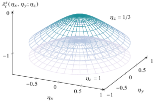
Figure 1: Plot of the eigenvalue $\lambda^{s}_{i}$ of $\eta_{x}\textbf{{A}}^{x}+\eta_{y}\textbf{{A}}^{y}+\eta_{z}\textbf{{A}}^{z}$ for varying $\eta_{x}$ and $\eta_{y}$ and fixed $\eta_{z}$. The plotted $\lambda^{s}_{i}$ corresponds to the eigenvalue $\lambda_{i}=-0.9062$ of $\textbf{{A}}^{x}$ with $l_{\text{max}}=4$ . The depicted circular hyperboloid is described by $(\eta^{2}_{x}+\eta^{2}_{y})/\eta^{2}_{z}-(\lambda^{s}_{i}/\lambda_{i}\eta_{z})^{2}=-1$.

The eigenvectors of the sum of the representation matrices (6.16) are the rotated eigenvectors of $\textbf{{A}}^{x}$, because

$$\eta\textbf{{A}}^{x}\textbf{{W}}^{x}=\eta\textbf{{W}}^{x}\bm{\Lambda}\iff\eta\textbf{{U}}(\alpha\textbf{{r}})\textbf{{A}}^{x}\textbf{{U}}^{\bm{\dagger}}(\alpha\textbf{{r}})\textbf{{U}}(\alpha\textbf{{r}})\textbf{{W}}^{x}=\eta\textbf{{U}}(\alpha\textbf{{r}})\textbf{{W}}^{x}\bm{\Lambda}\iff\left(\eta_{x}\textbf{{A}}^{x}+\eta_{y}\textbf{{A}}^{y}+\eta_{z}\textbf{{A}}^{z}\right)\textbf{{U}}(\alpha\textbf{{r}})\textbf{{W}}^{x}=\textbf{{U}}(\alpha\textbf{{r}})\textbf{{W}}^{x}\bm{\Lambda}^{s}\,.$$ (6.21)

We conclude this section with referring the reader to Garrett & Hauck (2016), who also investigated the eigenstructure of the $\textbf{{A}}^{a}$ matrices in the context of radiation transport and found similar results. Our work differs from theirs mainly in identifying the unitary matrices U as rotation matrices. Furthermore we would like to remark, that the eigenvalues of the real matrices $\textbf{{A}}^{a}_{R}$ are the same as the eigenvalues of the $\textbf{{A}}^{a}$ matrices, because $\textbf{{S}}^{\bm{\dagger}}\textbf{{A}}^{a}\textbf{{S}}=\textbf{{A}}^{a}_{R}$ is a similarity transformation.

7 Conclusions

The transport of particles or photons is very often modelled using variants of the Boltzmann equation. In many cases the scattering (or collision) operator has a particular simple form in the centre-of-momentum frame. This motivates to formulate the transport equation in a mixed-coordinate frame, i.e. a frame in which time and the configuration space variable x are measured in an inertial frame whereas p is given with respect to a non-inertial frame moving with the centre-of-momentum of the scattering centres. To render the equation amenable to be solved numerically, the single particle phase-space density is expanded in terms of known functions, for example the Legendre polynomials, to reduce the number of independent variables. This expansion leads to a system of partial differential equations evolving the expansion coefficients.

In this paper, a new method to derive this system of equations for the case of a spherical harmonic expansion of the single particle phase-space density has been presented. The method is based on operators acting on the space of spherical harmonics and their matrix representations. It was shown that the system is readily obtained by replacing the introduced and identified operators appearing in the VFP equation with their matrix representations. The final result is a compact matrix equation for the (real) expansion coefficients, which has the same structure and physical interpretation as the original VFP equation, i.e.

$$\begin{split}&\qquad\left(\textbf{{1}}+\frac{V}{c^{2}}U_{a}\textbf{{A}}^{a}_{R}\right)\partial_{t}\textbf{{f}}_{R}+\left(U^{a}\textbf{{1}}+V\textbf{{A}}^{a}_{R}\right)\partial_{x_{a}}\textbf{{f}}_{R}-\left(\gamma m\frac{\mathrm{d}U_{a}}{\mathrm{d}t}\textbf{{A}}^{a}_{R}+p\frac{\partial U_{b}}{\partial x^{a}}\textbf{{A}}^{a}_{R}\textbf{{A}}^{b}_{R}\right)\partial_{p}\textbf{{f}}_{R}\\ &\qquad\,\,\,\,\,{}+\left(\frac{1}{V}\epsilon_{abc}\frac{\mathrm{d}U^{a}}{\mathrm{d}t}\textbf{{A}}^{b}_{R}\bm{\Omega}^{c}_{R}+\epsilon_{bcd}\frac{\partial U_{b}}{\partial x^{a}}\textbf{{A}}^{a}_{R}\textbf{{A}}^{c}_{R}\bm{\Omega}^{d}\right)\textbf{{f}}_{R}-\omega_{a}\bm{\Omega}^{a}_{R}\textbf{{f}}_{R}+\nu\textbf{{C}}_{R}\textbf{{f}}_{R}=0\,.\end{split}$$ (7.1)

We simplified the computation of the matrix representations considerable with the help of rotations of the coordinate system in momentum space, see in particular eqs. (4.8), (4.9) and (4.11). We showed that the system of equations can be constructed from four representation matrices of whom two are diagonal and well-known.

The fact that the spherical harmonics (and the expansion coefficients) are complex whereas the single particle phase-space density is real, implies that the constructed system of equations contains linear dependent equations. We removed the redundant equations by multiplying the system with a basis transformation matrix, which turns the complex spherical harmonics into the real spherical harmonics, see eq. (5.7).

Eventually, we prepared the application of numerical methods, like the discontinuous Galerkin method or the finite volume method, through an investigation of the eigenvalues and eigenvectors of the representation matrices. A key insight consists in the fact that all representation matrices of the direction operators have the same eigenvalues. This holds true for the representations matrices of the angular momentum operators as well. Moreover, all eigenvalues are real. This was shown in Section (6.1). We emphasise, that we have proven that the eigenvalues of the representation matrices of the direction operators are the roots of the associated Legendre polynomials, see Section 6.2. We were also able to directly compute the eigenvalues and eigenvectors of the sum of the representation matrices of the direction operators, see eq. (6.20) and eq. (6.21). These results have all been exploited in the implementation of the Sapphire++ code, a discontinuous Galerkin scheme that solves equation (7.1). The details are described in a companion paper.

We conclude with two remarks: First, the presented method can be applied whenever a spherical harmonic expansion of the single particle phase-space density function is used. In particular, it is not necessary to formulate the transport equation in a mixed-coordinate frame. The only prerequisite is the ability to compute the representation matrix of the collision operator $\hat{C}$. Secondly, the presented operator method could be adapted to other expansions of the single particle phase-space density function as well.

Data Availability

Data sharing not applicable to this article as no datasets were generated or analysed during the current study.

Supplementary material

A free and open-source python script, which may serve as a reference implementation of the representation matrices, is available as supplementary material and at https://github.com/nils-schween/representation-matrices.

Appendix A Spherical harmonics

We would like to explicitly define the spherical harmonics, namely

$$Y^{m}_{l}(\theta,\varphi)=N^{m}_{l}P^{m}_{l}(\cos\theta)e^{\mathrm{i}m\varphi}\quad\text{with }N^{m}_{l}=\sqrt{\frac{2l+1}{4\pi}\frac{(l-m)!}{(l+m)!}}\,.$$ (A.1)

The functions $P^{m}_{l}$ are the associated Legendre Polynomials and we decided to use the following definition:

$$P^{m}_{l}(\cos\theta)=(-1)^{m}\sin^{m}\theta\frac{\mathrm{d}^{m}}{\mathrm{d}(\cos\theta)^{m}}P_{l}(\cos\theta)\,.$$ (A.2)

Note that the Condon–Shortley phase $(-1)^{m}$ is included in the definition of the associated Legendre polynomials and not in the definition of the spherical harmonics. The $P_{l}$ are the Legendre polynomials, which for example are defined to be the set of orthogonal polynomials on the interval $[-1,1]$ with the weight function $w(x)=1$, and can be constructed by an application of the Gram-Schmidt process to the monomials.

Appendix B Real representation matrices

At the end of Section (5.2), we referred the reader to the Appendix for a proof that the representation matrices corresponding to the real spherical harmonics are real.

We prove this statement by explicitly computing all the appearing matrices, i.e. we evaluate the matrix-matrix products in $\textbf{{S}}^{\bm{\dagger}}\textbf{{O}}\textbf{{S}}$. Where O is a representation matrix with respect to the complex spherical harmonics of an arbitrary operator.

The matrix elements of the inverse basis transformation are

$$\begin{split}(\textbf{{S}}^{\bm{\dagger}})_{i(l^{\prime},m^{\prime},s^{\prime})j(l,m)}&=\delta_{ll^{\prime}}\left(\frac{\delta_{mm^{\prime}}+(-1)^{m^{\prime}}\delta_{-m^{\prime}m}}{\sqrt{2(1+\delta_{m^{\prime}0})}}\delta_{s^{\prime}0}+\frac{\mathrm{i}(\delta_{mm^{\prime}}-(-1)^{m^{\prime}}\delta_{-m^{\prime}m})}{\sqrt{2}}\delta_{s^{\prime}1}\right)\,.\end{split}$$ (B.1)

We now demonstrate how to compute the matrix representation of an arbitrary operator $\hat{O}$ corresponding to the real spherical harmonics. We assume that we know its matrix representation with the respect to the complex spherical harmonics. Evaluating the necessary matrix-matrix products yields

$$\begin{split}&(\textbf{{O}}_{R})_{i(l^{\prime},m^{\prime},s^{\prime})j(l,m,s)}\\ &\qquad=\sum_{n,k}\sum_{n^{\prime},k^{\prime}}(\textbf{{S}}^{\bm{\dagger}})_{i(l^{\prime},m^{\prime},s^{\prime})h(n,k)}\textbf{{O}}_{h(n,k)r(n^{\prime},k^{\prime})}(\textbf{{S}})_{r(n^{\prime},k^{\prime})j(l,m,s)}\\ &\qquad=\sum_{n,k}\sum_{n^{\prime},k^{\prime}}\delta_{l^{\prime}n}\delta_{ln^{\prime}}\left(\frac{\delta_{m^{\prime}k}+(-1)^{m^{\prime}}\delta_{-m^{\prime}k}}{\sqrt{2(1+\delta_{m^{\prime}0})}}\delta_{s^{\prime}0}+\frac{\mathrm{i}(\delta_{m^{\prime}k}-(-1)^{m^{\prime}}\delta_{-m^{\prime}k})}{\sqrt{2}}\delta_{s^{\prime}1}\right)\textbf{{O}}_{h(n,k)r(n^{\prime},k^{\prime})}\\ &\qquad\phantom{=}{}\times\left(\frac{\delta_{mk^{\prime}}+(-1)^{m}\delta_{-mk^{\prime}}}{\sqrt{2(1+\delta_{m0})}}\delta_{s0}-\frac{\mathrm{i}(\delta_{mk^{\prime}}-(-1)^{m}\delta_{-mk^{\prime}})}{\sqrt{2}})\delta_{s1}\right)\\ &\qquad=\frac{1}{2}\frac{\delta_{s^{\prime}0}\delta_{s0}}{\sqrt{(1+\delta_{m^{\prime}0})(1+\delta_{m0})}}\left(\textbf{{O}}_{i(l^{\prime},m^{\prime})j(l,m)}+(-1)^{m^{\prime}}\textbf{{O}}_{i(l^{\prime},-m^{\prime})j(l,m)}+(-1)^{m}\textbf{{O}}_{i(l^{\prime},m^{\prime})j(l,-m)}+(-1)^{m^{\prime}+m}\textbf{{O}}_{i(l^{\prime},-m^{\prime})j(l,-m)}\right)\\ &\qquad\phantom{=}{}-\frac{\mathrm{i}}{2}\frac{\delta_{s^{\prime}0}\delta_{s1}}{\sqrt{(1+\delta_{m^{\prime}0})}}\left(\textbf{{O}}_{i(l^{\prime},m^{\prime})j(l,m)}+(-1)^{m^{\prime}}\textbf{{O}}_{i(l^{\prime},-m^{\prime})j(l,m)}-(-1)^{m}\textbf{{O}}_{i(l^{\prime},m^{\prime})j(l,-m)}-(-1)^{m^{\prime}+m}\textbf{{O}}_{i(l^{\prime},-m^{\prime})j(l,-m)}\right)\\ &\qquad\phantom{=}{}+\frac{\mathrm{i}}{2}\frac{\delta_{s^{\prime}1}\delta_{s0}}{\sqrt{(1+\delta_{m0})}}\left(\textbf{{O}}_{i(l^{\prime},m^{\prime})j(l,m)}-(-1)^{m^{\prime}}\textbf{{O}}_{i(l^{\prime},-m^{\prime})j(l,m)}+(-1)^{m}\textbf{{O}}_{i(l^{\prime},m^{\prime})j(l,-m)}-(-1)^{m^{\prime}+m}\textbf{{O}}_{i(l^{\prime},-m^{\prime})j(l,-m)}\right)\\ &\qquad\phantom{=}{}+\frac{1}{2}\delta_{s^{\prime}1}\delta_{s1}\left(\textbf{{O}}_{i(l^{\prime},m^{\prime})j(l,m)}-(-1)^{m^{\prime}}\textbf{{O}}_{i(l^{\prime},-m^{\prime})j(l,m)}-(-1)^{m}\textbf{{O}}_{i(l^{\prime},m^{\prime})j(l,-m)}+(-1)^{m^{\prime}+m}\textbf{{O}}_{i(l^{\prime},-m^{\prime})j(l,-m)}\right)\,.\\ \end{split}$$ (B.2)

Having derived an expression for the real matrix representation for an arbitrary operator, we can apply it to the angular momentum operators, the direction operators, the collision operator and the rotation operators. We note that $\mathbf{O}_{R}$ contains complex terms and, thus, we have to check if the resulting representation matrices corresponding to the above list of operators are real.

When computing the matrix representations with respect to the real spherical harmonics, it is important to note that $m^{\prime},m\geq 0$, hence $\delta_{-m^{\prime}(m+1)}=\delta_{m^{\prime}(-m-1)}=0$ and $\delta_{-m^{\prime}(m-1)}=\delta_{m^{\prime}(-m+1)}=\delta_{m^{\prime}0}\delta_{m1}+\delta_{m^{\prime}1}\delta_{m0}$. Moreover, $m^{\prime}=0$ and $s^{\prime}=1$ (or $m=0$ and $s=1$) is excluded6, which we use to remove terms from the resulting expressions. Generally, we remove terms with combinations of Kronecker deltas whose evaluation leads to values of $l,m$ and $s$ which are not allowed.

We begin with the representation matrices of the angular momentum operator. We remind ourselves that we have to include a factor $\mathrm{i}$, because $\bm{\Omega}^{a}_{R}=\mathrm{i}\textbf{{S}}^{\bm{\dagger}}\bm{\Omega}^{a}\textbf{{S}}$. Using eq. (B.2) yields

$$\begin{split}&(\bm{\Omega}^{x}_{R})_{i(l^{\prime},m^{\prime},s^{\prime})j(l,m,s)}\\ &\qquad=m\delta_{l^{\prime}l}\delta_{m^{\prime}m}\left(\frac{\delta_{s^{\prime}0}\delta_{s1}}{\sqrt{1+\delta_{m^{\prime}0}}}-\frac{\delta_{s^{\prime}1}\delta_{s0}}{\sqrt{1+\delta_{m0}}}\right)=\bm{\Omega}^{x}_{i(l^{\prime},m^{\prime})j(l,m)}\left(\frac{\delta_{s^{\prime}0}\delta_{s1}}{\sqrt{1+\delta_{m^{\prime}0}}}-\frac{\delta_{s^{\prime}1}\delta_{s0}}{\sqrt{1+\delta_{m0}}}\right)\\ &(\bm{\Omega}^{y}_{R})_{i(l^{\prime},m^{\prime},s^{\prime})j(l,m,s)}\\ &\qquad=\frac{\delta_{l^{\prime}l}}{2}\Biggl{[}\Biggr{.}\frac{\delta_{s^{\prime}0}\delta_{s1}}{\sqrt{1+\delta_{m^{\prime}0}}}\left(\sqrt{(l+m+1)(l-m)}\delta_{m^{\prime}(m+1)}+\sqrt{(l+m)(l-m+1)}\delta_{m^{\prime}(m-1)}+\sqrt{l(l+1)}\delta_{m^{\prime}0}\delta_{m1}\right)\\ &\qquad\phantom{=}\qquad\,\,\Biggl{.}{}-\frac{\delta_{s^{\prime}1}\delta_{s0}}{\sqrt{1+\delta_{m0}}}\left(\sqrt{(l+m+1)(l-m)}\delta_{m^{\prime}(m+1)}+\sqrt{(l+m)(l-m+1)}\delta_{m^{\prime}(m-1)}+\sqrt{l(l+1)}\delta_{m^{\prime}1}\delta_{m0}\right)\Biggr{]}\\ &\qquad=\frac{\delta_{s^{\prime}0}\delta_{s1}}{\sqrt{1+\delta_{m^{\prime}0}}}\left(\bm{\Omega}^{y}_{i(l^{\prime},m^{\prime})j(l,m)}+\frac{\delta_{l^{\prime}l}}{2}\sqrt{l(l+1)}\delta_{m^{\prime}0}\delta_{m1}\right)-\frac{\delta_{s^{\prime}1}\delta_{s0}}{\sqrt{1+\delta_{m0}}}\left(\bm{\Omega}^{y}_{i(l^{\prime},m^{\prime})j(l,m)}+\frac{\delta_{l^{\prime}l}}{2}\sqrt{l(l+1)}\delta_{m^{\prime}1}\delta_{m0}\right)\\ &(\bm{\Omega}^{z}_{R})_{i(l^{\prime},m^{\prime},s^{\prime})j(l,m,s)}\\ &\qquad=\frac{\delta_{l^{\prime}l}}{2}\Biggl{[}\Biggr{.}\frac{\delta_{s^{\prime}0}\delta_{s0}}{\sqrt{(1+\delta_{m^{\prime}0})(1+\delta_{m0})}}\left(\sqrt{(l+m+1)(l-m)}\delta_{m^{\prime}(m+1)}-\sqrt{(l+m)(l-m+1)}\delta_{m^{\prime}(m-1)}-\sqrt{l(l+1)}(\delta_{m^{\prime}0}\delta_{m1}-\delta_{m^{\prime}1}\delta_{m0})\right)\\ &\qquad\phantom{=}\qquad\,\,\Biggl{.}{}+\delta_{s^{\prime}1}\delta_{s1}\left(\sqrt{(l+m+1)(l-m)}\delta_{m^{\prime}(m+1)}-\sqrt{(l+m)(l-m+1)}\delta_{m^{\prime}(m-1)}\right)\Biggr{]}\\ &\qquad=\frac{\delta_{s^{\prime}0}\delta_{s0}}{\sqrt{(1+\delta_{m^{\prime}0})(1+\delta_{m0})}}\left(\mathrm{i}\bm{\Omega}^{z}_{i(l^{\prime},m^{\prime})j(l,m)}-\frac{\delta_{l^{\prime}l}}{2}\sqrt{l(l+1)}(\delta_{m^{\prime}0}\delta_{m1}-\delta_{m^{\prime}1}\delta_{m0})\right)+\delta_{s^{\prime}1}\delta_{s1}\mathrm{i}\bm{\Omega}^{z}_{i(l^{\prime},m^{\prime})j(l,m)}\end{split}$$ (B.3)

We proceed with the matrix representations of the direction operators $\hat{A}^{a}$ operators. We find that

$$\begin{split}&(\textbf{{A}}^{x}_{R})_{i(l^{\prime},m^{\prime},s^{\prime})j(l,m,s)}\\ &\qquad=\delta_{m^{\prime}m}\delta_{s^{\prime}s}\left(\sqrt{\frac{(l+m+1)(l-m+1)}{(2l+3)(2l+1)}}\delta_{l^{\prime}(l+1)}+\sqrt{\frac{(l+m)(l-m)}{(2l+1)(2l-1)}}\delta_{l^{\prime}(l-1)}\right)=\delta_{s^{\prime}s}\textbf{{A}}^{x}_{i(l^{\prime},m^{\prime})j(l,m)}\\ &(\textbf{{A}}^{y}_{R})_{i(l^{\prime},m^{\prime},s^{\prime})j(l,m,s)}\\ &\qquad=\frac{\delta_{s^{\prime}0}\delta_{s0}}{\sqrt{(1+\delta_{m^{\prime}0})(1+\delta_{m0})}}\left((\textbf{{A}}^{y})_{i(l^{\prime},m^{\prime})j(l,m)}+\frac{1}{2}\left(a^{-m+1}_{l+1}\delta_{l^{\prime}(l+1)}-a^{m}_{l}\delta_{l^{\prime}(l-1)}\right)(\delta_{m^{\prime}0}\delta_{m1}-\delta_{m^{\prime}1}\delta_{m0})\right)+\delta_{s^{\prime}1}\delta_{s1}(\textbf{{A}}^{y})_{i(l^{\prime},m^{\prime})j(l,m)}\\ &(\textbf{{A}}^{z}_{R})_{i(l^{\prime},m^{\prime},s^{\prime})j(l,m,s)}\\ &\qquad=\frac{\delta_{s^{\prime}0}\delta_{s1}}{\sqrt{1+\delta_{m^{\prime}0}}}\left(-\mathrm{i}(\textbf{{A}}^{z})_{i(l^{\prime},m^{\prime})j(l,m)}+\frac{1}{2}\left(a^{-m+1}_{l+1}\delta_{l^{\prime}(l+1)}-a^{m}_{l}\delta_{l^{\prime}(l-1)}\right)\delta_{m^{\prime}0}\delta_{m1}\right)\\ &\qquad\phantom{=}{}-\frac{\delta_{s^{\prime}1}\delta_{s0}}{\sqrt{1+\delta_{m0}}}\left(-\mathrm{i}(\textbf{{A}}^{z})_{i(l^{\prime},m^{\prime})j(l,m)}+\frac{1}{2}\left(a^{-m+1}_{l+1}\delta_{l^{\prime}(l+1)}-a^{m}_{l}\delta_{l^{\prime}(l-1)}\right)\delta_{m^{\prime}1}\delta_{m0}\right)\end{split}$$ (B.4)

We point out that $\textbf{{A}}^{x}=\textbf{{A}}^{x}_{R}$.

The same is true for the real representation matrix of the collision operator $\hat{C}$, which is

$$(\textbf{{C}}_{R})_{i(l^{\prime}m^{\prime}s^{\prime})j(l,m,s)}=\frac{l(l+1)}{2}\delta_{l^{\prime}l}\delta_{m^{\prime}m}\delta_{s^{\prime}s}\,.$$ (B.5)

It is left to compute the real representation matrices of the used rotation operators, i.e. $e^{\mathrm{i}\frac{\pi}{2}\hat{L}_{x}}$ and $e^{\mathrm{i}\frac{\pi}{2}\hat{L}_{z}}$. They are

$$\begin{split}(\textbf{{U}}_{R}(-\pi/2\textbf{{e}}_{x}))_{i(l^{\prime},m^{\prime},s^{\prime})j(l,m,s)}&=e^{\frac{\pi}{2}\bm{\Omega}^{x}_{R}}\\ &=\delta_{l^{\prime}l}\delta_{m^{\prime}m}\left[\frac{\delta_{s^{\prime}0}\delta_{s0}}{\sqrt{(1+\delta_{m^{\prime}0})(1+\delta_{m0})}}\left(\cos\left(\frac{\pi}{2}m\right)+1\delta_{m^{\prime}0}\delta_{m0}\right)+\frac{\delta_{s^{\prime}1}\delta_{s0}}{\sqrt{1+\delta_{m^{\prime}0}}}\sin\left(\frac{\pi}{2}m\right)\right.\\ &\phantom{=\delta_{l^{\prime}l}\delta_{m^{\prime}m}}\left.\,\,\,{}-\frac{\delta_{s^{\prime}0}\delta_{s1}}{\sqrt{1+\delta_{m0}}}\sin\left(\frac{\pi}{2}m\right)+\delta_{s^{\prime}1}\delta_{s1}\cos\left(\frac{\pi}{2}m\right)\right]\\ (\textbf{{U}}_{R}(-\pi/2\textbf{{e}}_{z}))_{i(l^{\prime},m^{\prime},s^{\prime})j(l,m,s)}&=e^{\frac{\pi}{2}\bm{\Omega}^{z}_{R}}\\ &=\Biggl{[}\frac{\delta_{s^{\prime}0}\delta_{s0}}{\sqrt{(1+\delta_{m^{\prime}0})(1+\delta_{m0})}}\left((\textbf{{U}}(-\pi/2\textbf{{e}}_{z})_{i(l^{\prime},m^{\prime})j(l,m)}+(-1)^{m}\textbf{{U}}(-\pi/2\textbf{{e}}_{z})_{i(l^{\prime},m^{\prime})j(l,-m)})\right)\Biggr{.}\\ &\phantom{=}\Biggl{.}\,\,\,{}+\delta_{s^{\prime}1}\delta_{s1}\left((\textbf{{U}}(-\pi/2\textbf{{e}}_{z})_{i(l^{\prime},m^{\prime})j(l,m)}-(-1)^{m}\textbf{{U}}(-\pi/2\textbf{{e}}_{z})_{i(l^{\prime},m^{\prime})j(l,-m)})\right)\Biggr{]}\end{split}$$ (B.6)

For the last equation we assumed that $\textbf{{U}}_{R}(-\pi/2\textbf{{e}}_{z})$ is real, which is of course against the idea to prove that it is real. Since $\textbf{{U}}(-\pi/2\textbf{{e}}_{z})$ is real as well, we concluded that the two terms in middle of eq. (B.2) must be zero for $\textbf{{U}}_{R}(-\pi/2\textbf{{e}}_{z})$. This conclusion lead us to conjecture that $(-1)^{m^{\prime}}\textbf{{U}}(\pi/2\textbf{{e}}_{z})_{i(l^{\prime},-m^{\prime})j(l,m)}=(-1)^{m}\textbf{{U}}(-\pi/2\textbf{{e}}_{z})_{i(l^{\prime},m^{\prime})j(l,-m)}$ and that $\textbf{{U}}(-\pi/2\textbf{{e}}_{z})_{i(l^{\prime},m^{\prime})j(l,m)}=(-1)^{m^{\prime}+m}\textbf{{U}}(-\pi/2\textbf{{e}}_{z})_{i(l^{\prime},m^{\prime})j(l,-m)}$. These conjectures give us the above result and numerical experiments convinced us that these conjectures are true.

References

• Achterberg & Norman (2018) Achterberg A., Norman C. A., 2018, MNRAS, 479, 1747
• Bell et al. (2006) Bell A. R., Robinson A. P. L., Sherlock M., Kingham R. J., Rozmus. W., 2006, Plasma Physics and Controlled Fusion, 48, R37
• Braginskii (1958) Braginskii S. I., 1958, Soviet Journal of Experimental and Theoretical Physics, 6, 358
• Castor (1972) Castor J. I., 1972, ApJ, 178, 779
• Chandrasekhar (1960) Chandrasekhar S., 1960, Radiative transfer. Dover
• Fakhri (2016) Fakhri H., 2016, Advances in High Energy Physics, 2016, 7
• Garrett & Hauck (2016) Garrett C. K., Hauck C. D., 2016, Computers & Mathematics with Applications, 72, 264
• Ginzburg & Syrovatskii (1964) Ginzburg V. L., Syrovatskii S. I., 1964, The Origin of Cosmic Rays. Pergamon Press Ltd.
• Jeevanjee (2011) Jeevanjee N., 2011, An Introduction to Tensors and Group Theory for Physicists, 2 edn. Birkhäuser, doi:10.1007/978-0-8176-4715-5
• Johnston (1960) Johnston T. W., 1960, Physical Review, 120, 1103
• Kirk & Schneider (1987) Kirk J. G., Schneider P., 1987, ApJ, 315, 425
• Kirk et al. (1988) Kirk J. G., Schlickeiser R., Schneider P., 1988, ApJ, 328, 269
• Kirk et al. (2023) Kirk J. G., Reville B., Huang Z.-Q., 2023, MNRAS, 519, 1022
• Landau & Lifshitz (1977) Landau L., Lifshitz E., 1977, Quantum Mechanics. Non-Relativistic Theory, 3 edn. Pergamon Press
• Lewis & Miller (1984) Lewis E. E., Miller W. F., 1984, Computational methods of neutron transport. John Wiley and Sons, Inc., New York, NY
• Lindquist (1966) Lindquist R. W., 1966, Annals of Physics, 37, 487
• Melrose (1969) Melrose D. B., 1969, Ap&SS, 4, 143
• Mihalas & Mihalas (1984) Mihalas D., Mihalas B. W., 1984, Foundations of radiation hydrodynamics. Oxford University Press
• Milton & Stegun (1964) Milton A., Stegun I. A., 1964, Handbook of Mathematical Functions with Formulas Graphs and Mathematical Tables, 10th print. 1972, with corrections edn. U.S. Dept. of Commerce National Bureau of Standards
• Reville & Bell (2013) Reville B., Bell A. R., 2013, MNRAS, 430, 2873
• Riffert (1986) Riffert H., 1986, ApJ, 310, 729
• Rosenbluth et al. (1957) Rosenbluth M. N., MacDonald W. M., Judd D. L., 1957, Physical Review, 107, 1
• Schween & Reville (2022) Schween N. W., Reville B., 2022, Journal of Plasma Physics, 88, 905880510
• Shkarofsky et al. (1966) Shkarofsky I., Johnston T., Bachynski M., 1966, The Particle Kinetics of Plasmas. Addison-Wesley, Reading, Massachusetts
• Skilling (1975) Skilling J., 1975, MNRAS, 172, 557
• Thomas et al. (2012) Thomas A., Tzoufras M., Robinson A., Kingham R., Ridgers C., Sherlock M., Bell A., 2012, Journal of Computational Physics, 231, 1051–1079
• Thorne (1980) Thorne K. S., 1980, Reviews of Modern Physics, 52, 299–339
• Thorne (1981) Thorne K. S., 1981, Monthly Notices of the Royal Astronomical Society, 194, 439–473
• Tricomi (1950) Tricomi F. G., 1950, Annali di Matematica Pura ed Applicata, 31, 93
• Tzoufras et al. (2011) Tzoufras M., Bell A., Norreys P., Tsung F., 2011, Journal of Computational Physics, 230, 6475
• Varshalovich et al. (1988) Varshalovich D. A., Moskalev A. N., Khersonskii V. K., 1988, Quantum Theory of Angular Momentum. World Scientific, doi:10.1142/0270
• Webb (1985) Webb G. M., 1985, ApJ, 296, 319
• Webb (1987) Webb G. M., 1987, The Astrophysical Journal, 321, 606
• Webb (1989) Webb G. M., 1989, The Astrophysical Journal, 340, 1112
• Williams & Jokipii (1991) Williams L. L., Jokipii J. R., 1991, ApJ, 371, 639