Strong coupling yields abrupt synchronization transitions in coupled oscillators

Abstract

Coupled oscillator networks often display transitions between qualitatively different phase-locked solutions—such as synchrony and rotating wave solutions—following perturbation or parameter variation. In the limit of weak coupling, these transitions can be understood in terms of commonly studied phase approximations. As the coupling strength increases, however, predicting the location and criticality of transition, whether continuous or discontinuous, from the phase dynamics may depend on the order of the phase approximation—or a phase description of the network dynamics that neglects amplitudes may become impossible altogether. Here we analyze synchronization transitions and their criticality systematically for varying coupling strength in theory and experiments with coupled electrochemical oscillators. First, we analyze bifurcations analysis of synchrony and splay states in an abstract phase model and discuss conditions under which synchronization transitions with different criticalities are possible. Second, we illustrate that transitions with different criticality indeed occur in experimental systems. Third, we highlight that the amplitude dynamics observed in the experiments can be captured in a numerical bifurcation analysis of delay-coupled oscillators. Our results showcase that reduced order phase models may miss important features that one would expect in the dynamics of the full system.

I Introduction

Collective oscillatory dynamics are a hallmark of a multitude of real world networks, such as electrical activity in the brain Ashwin et al. (2016); Bick et al. (2020), power grids Filatrella et al. (2008); Dörfler et al. (2013), and epidemiology Yan et al. (2007); Gross and Kevrekidis (2008). Such systems are often described using network dynamical systems models that couple together nodes that each intrinsically (i.e., in the absence of coupling) exhibit stable, hyperbolic limit cycle oscillations. If the oscillation frequencies of the nodes, or subsets of nodes, are sufficiently close together, the network can display phase-locked behaviour in which the phase difference between pairs of nodes converges to a finite value Hoppensteadt and Izhikevich (1997). As parameters, such as the coupling strength, are varied, networks may exhibit sharp transitions between collective oscillations with different phase-difference properties. Particularly striking examples include the abrupt synchronization phenomenon in which a group of nodes (potentially encompassing the entire network) exhibits a sharp transition from an incoherent state to a phase-locked state in which the phase differences between nodes in the group vanishes Zhang et al. (2014); Vlasov et al. (2015).

If the coupling is sufficiently weak, the network dynamics can be described using phase reduction Nakao (2016); Pietras and Daffertshofer (2019). The phase reduction describes the dynamics of the phases on an attracting invariant torus in terms of intrinsic rotation and a phase interaction function that captures how the oscillators’ phases interact. To first order, the phase interaction function is a convolution of the phase response function, which captures the linear sensitivity of the phase of a node oscillation to a perturbation, and a coupling function that describes how nodes interact with one another. These functions can often be inferred from data, or estimated using perturbative experiments. This makes weakly coupled oscillator theory an attractive framework for studying real world systems, for example to design the dynamics of coupled oscillator networks Kori et al. (2008); Kiss (2018).

If the coupling between individual units becomes strong—as is the case in many real-world systems—the assumptions that underlie phase reduction cease to be satisfied. It is thus pertinent to ask which predictions of the weakly coupled theory break as the coupling strength is increased and how such predictions change. For example, strong coupling may turn a continuous synchronization transition into a discontinuous one Călugăru et al. (2020). Recent work has demonstrated that predictions for infinitesimal coupling strengths are inconsistent with those for small, finite coupling strengths, even for simple oscillator models Börgers (2023). Similarly, perturbations to oscillation amplitudes can impact phase dynamics, particularly, if the amplitudes of different node oscillations are perturbed in different ways. For example, it has long been known that chaotic dynamics with small amplitude variation can emerge close to bifurcations of coupled oscillator networks as the coupling strength is increased due to the presence of symmetries in the underlying dynamics in what is known as instant chaos Guckenheimer and Worfolk (1992).

To understand network dynamics beyond the weak coupling limit, new mathematical tools have recently become available. On the one hand, these include higher-order phase reductions, that give a more accurate description of the phase dynamics Skardal and Arenas (2020); Bick et al. (2023). On the other hand, one can derive approximations that allow for additional degrees of freedom. For example, phase-amplitude reductions adds a degree of freedom that corresponds to an “amplitude” variable; cf. Wedgwood et al. (2013); Wilson and Moehlis (2016); Letson and Rubin (2018); Wilson and Ermentrout (2019). Such approximations have also been derived for dynamical systems with time delay Kotani et al. (2012). Despite being ad-hoc and without a rigorous mathematical justification, there have been promising results showcasing the merits of these frameworks, including demonstrations of how amplitude variations can be controlled Wilson (2020). However, it remains an open question how best to incorporate the effects of strong coupling in a practical sense.

Here, we take an interdisciplinary approach to elucidate the effect of strong coupling on the synchronization dynamics in a minimal network of two delay-coupled phase oscillators. Specifically, we demonstrate how abrupt transitions between different phase-locked states of a two-node network are induced by changes in coupling strength. First, we consider phase dynamics for two coupled oscillators with higher harmonics. Here, one would expect higher harmonics to shape the dynamics for highly nonsinusoidal oscillations as the coupling strength is increased. We show that higher harmonics can introduce changes in the criticality of key bifurcations, which in turn leads to bistability between solutions with different asymptotic phase differences. Second, we demonstrate that such transitions arise in experiments involving a network of electrochemical oscillators coupled through delayed feedback. Since the phase theory is insufficient to describe amplitude variations observed in the experiments, we investigate a network of two delay-coupled oscillators through numerical bifurcation analysis of a model of the chemical oscillator network. Here, we demonstrate the existence of branches of symmetry-broken solutions that are well-matched to the experimental observations.

II Continuous and discontinuous transitions between synchronized states in phase oscillators

To understand transitions between in-phase and anti-phase dynamics, we consider the simple case of a network of two delay-coupled nonlinear oscillators. Specifically, the state of each oscillator is given by $x_{k}\in\mathbb{R}^{N}$ and evolves according to

$$\dot{x}_{1} =F(x_{1})+KG(x_{2}(t-\tau)),$$ (1a)

$$\dot{x}_{2} =F(x_{2})+KG(x_{1}(t-\tau)),$$ (1b)

where $F:\mathbb{R}^{N}\to\mathbb{R}^{N}$ determines the intrinsic oscillatory dynamics and $G:\mathbb{R}^{N}\to\mathbb{R}^{N}$ determines the interactions with strength $K\geq 0$ and delay $\tau\geq 0$. In the uncoupled case, with $K=0$, each node possesses a stable hyperbolic limit cycle with intrinsic frequency $\omega$. If the coupling is sufficiently weak ($|K|\ll 1$), the dynamics of (1) evolve on an invariant torus in which the oscillator amplitudes are slaved to the respective oscillator phases $\theta_{1},\theta_{2}\in\mathbf{T}:=\mathbb{R}/2\pi\mathbb{Z}$. In this case, the dynamics can be simplified via projection onto this invariant torus Nakao (2016); Pietras and Daffertshofer (2019), so that the (averaged) phase equations for (1) with $n$ relevant harmonics can be written as

$$\dot{\theta}_{1} =\omega+g(\theta_{2}-\theta_{1}+\alpha),$$ (2a)

$$\dot{\theta}_{2} =\omega+g(\theta_{1}-\theta_{2}+\alpha),$$ (2b)

where

$$g(\phi)=\frac{1}{2}\sum_{m=1}^{n}{a_{j}}\sin(m\phi+\gamma_{m})$$ (3)

is the $2\pi$-periodic (phase) coupling function, and $\alpha$ is a phase shift parameter common to both oscillators. Up to rescaling, we may assume $a_{1}=1$ and $\gamma_{1}=0$. Note that, in the limit of weak coupling, the delay $\tau$ in (1) is associated with the phase shift $\alpha$ in (2), which, in turn, can affect the stability of the synchronized solutions and thus serves as a convenient bifurcation parameter that can be used to engineer phase differences between coupled oscillators Sakaguchi and Kuramoto (1986); Kori et al. (2008).

II.1 Symmetries, bifurcations, and criticality

By symmetry, the in-phase solution $\Theta_{0}=\{\theta_{1}=\theta_{2}\}$ and the anti-phase solution $\Theta_{\pi}=\{\theta_{1}=\theta_{2}+\pi\}$ are (relative) equilibria of (2) for any choice of parameter values. Note that (2) inherits the permutational symmetry $(\theta_{1},\theta_{2})\mapsto(\theta_{2},\theta_{1})$ from (1), and—since it describes the slow evolution of the phase differences—a continuous phase-shift symmetry where $\gamma\in\mathbf{T}$ acts by $\gamma:(\theta_{1},\theta_{2})\mapsto(\theta_{1}+\gamma,\theta_{2}+\gamma)$. To eliminate this phase shift symmetry, we can describe the dynamics of (2) in terms of the phase difference $\psi:=\theta_{2}-\theta_{1}$ between the two oscillators. The phase difference evolves according to

$$\begin{split}\dot{\psi}&=g(-\psi+\alpha)-g(\psi+\alpha)\\ &=\sum_{m=1}^{n}a_{m}\cos(m\alpha+\gamma_{m})\sin(m\psi).\end{split}$$ (4)

In-phase synchrony $\Theta_{0}$ in (2) corresponds to $\psi=0$ and anti-phase synchrony $\Theta_{\pi}$ corresponds to $\psi=\pi$; both of these points are equilibria of (4).

We now consider bifurcations of in-phase ($\psi=0$) and anti-phase ($\psi=\pi$) configurations as the phase-shift parameter $\alpha$ is varied. For coupling functions $g$ with a single nontrivial harmonic, i.e., $a_{j}=0$ for $j\geq 2$, both $\psi=0$ and $\psi=\pi$ bifurcate at $\alpha=\frac{\pi}{2}+q\pi$, $q\in\mathbb{Z}$ and are connected by a “vertical” branch of equilibria along which any $\psi\in\mathbf{T}$ is an equilibrium of (4). If the second harmonic is also non-zero, then there is a nondegenerate branch of equilibria around $\alpha=\frac{\pi}{2}$ that connects $\psi=0$ and $\psi=\pi$ Rusin et al. (2010); the bifurcations of these solutions are either both super- or both subcritical. While first and second harmonics may be a suitable approximation in certain parameter regimes (e.g., where $G$ describes linear coupling or when the uncoupled limit cycles are almost sinusoidal in nature), one expects that higher harmonics in the phase dynamics become more relevant in (2) as the coupling strength $K$ is increased.

It is then instructive to ask what the consequence of the presence of these higher harmonics might be for the phase dynamics. One specific important question is whether it is possible for the bifurcations of the in-phase ($\psi=0$) and anti-phase configurations ($\psi=\pi$) in (2) to have different criticality when higher harmonics are taken into account. While one can generically control the criticality of the transition locally Kuehn and Bick (2021), we consider in-phase and anti-phase configurations here simultaneously in the context of (2).

If the harmonics do not have distinct phase shifts, i.e., $\gamma_{m}=0$, then the criticality of the bifurcations of $\psi=0$ and $\psi=\pi$ are identical; this implies in particular that generalizing the phase interaction function considered in Rusin et al. (2010) to more than two nontrivial harmonics cannot give transitions of distinct criticality. This can be seen by noting that the system for $\gamma_{m}=0$ has a parameter symmetry $(\psi,\alpha)\mapsto(\pi-\psi,\pi-\alpha)$. This implies that $\psi=\frac{\pi}{2}$ is an equilibrium for $\alpha=\frac{\pi}{2}$ and that any bifurcation of $\psi=0$ at $\alpha=\hat{\alpha}$ leads to an identical bifurcation of $\psi=\pi$ at $\alpha=\pi-\hat{\alpha}$. Moreover, if all even harmonics vanish (i.e., $a_{m}$ = 0 for $m$ even), then $\psi=0$ and $\psi=\pi$ bifurcate at $\alpha=\frac{\pi}{2}$. Thus, if parameters are such that there is only a single bifurcation of $\psi=0,\pi$ for $\alpha\in(0,\pi)$ (i.e., these bifurcations are related by symmetry) then it is necessary to have non-zero $\gamma_{m}$ for the bifurcations to have distinct criticality.

II.2 Distinct criticality of transitions of in-phase and anti-phase configurations

We now consider the bifurcations of $\psi\in\{0,\pi\}$ in $\alpha$ for more general choices of $\gamma_{m}$. Expanding (4) around $\psi=0$ yields

$$\dot{\psi}=\sum_{m=1}^{n}a_{m}\cos(m\alpha+\gamma_{m})\left(m\psi-\frac{m^{3}\psi^{3}}{3!}+\dotsb\right).$$ (5)

Thus, the linear stability of $\psi=0$ as well as the criticality of the (potentially degenerate) pitchfork bifurcation around $\psi=0$ are determined by

$$D_{1}(0;\alpha) =\sum_{m=1}^{n}ma_{m}\cos(m\alpha+\gamma_{m}),$$ (6a)

$$D_{3}(0;\alpha) =-\frac{1}{3!}\sum_{m=1}^{n}m^{3}a_{m}\cos(m\alpha+\gamma_{m}).$$ (6b)

Specifically, solving $D_{1}(0;\alpha)=0$ for $\alpha$ determines a bifurcation point $\alpha^{(0)}$ of $\psi=0$ as $\alpha$ is varied and $D_{3}(0;\alpha^{(0)})$ determines the criticality of this transition. In particular, the bifurcation yields a continuous transition (a supercritical pitchfork bifurcation with an emerging branch of stable equilibria) if $D_{3}(0;\alpha^{(0)})<0$ and a discontinuous transition (a subcritical pitchfork bifurcation with an emerging branch of unstable equilibria) if $D_{3}(0;\alpha^{(0)})>0$. In a similar fashion, expanding (4) around $\psi=\pi$ gives

$$D_{1}(\pi;\alpha) =\sum_{m=1}^{n}(-1)^{m}ma_{m}\cos(m\alpha+\gamma_{m}),$$ (7a)

$$D_{3}(\pi;\alpha) =-\frac{1}{3!}\sum_{m=1}^{n}(-1)^{m}m^{3}a_{m}\cos(m\alpha+\gamma_{m}).$$ (7b)

Thus, the bifurcation of the anti-phase configuration $\psi=\pi$ at $\alpha^{(\pi)}$ is continuous if $D_{3}(\pi;\alpha^{(\pi)})<0$ and discontinuous if $D_{3}(\pi;\alpha^{(\pi)})>0$.

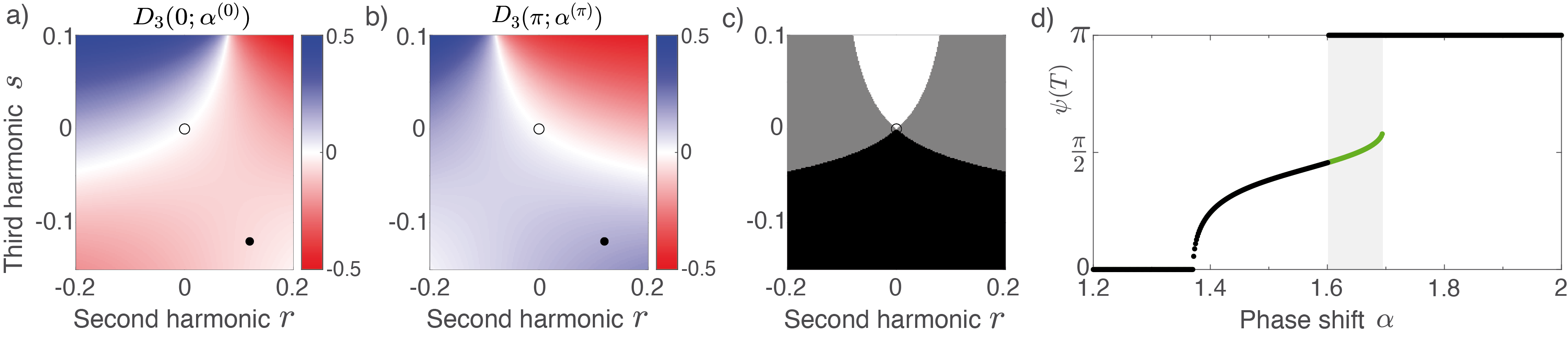
Figure 1: Varying parameters demonstrates regions in which the bifurcations of equilibria $\psi=0,\pi$ have distinct criticality. Results are demonstrated for fixed $\gamma_{2}=0.2$, $\gamma_{3}=0.5$. a) Criticality coefficient (6b) for $\psi=0$ as the strength $r,s$ of the second and third harmonic is varied; blue indicates a continuous, red a discontinuous transition; a hollow circle indicates $r=s=0$ and a filled circle the parameter values in panel d). b) Criticality coefficient (7b) for $\psi=\pi$ as in panel a). c) Regions in which the bifurcations of the in-phase and anti-phase configurations have distinct criticalities: white indicates that the transition at $\psi=0$ is continuous while $\psi=\pi$ is discontinuous and black vice versa. Bifurcations of $\psi=0$ and $\psi=\pi$ have the same criticality in the grey regions. d) Pseudocontinuation plot for $r=-s=0.12$ as the parameter $\alpha$ is increased (green) or decreased (black); an approximate region of hysteresis/multistability due to the discontinuous transition of the $\psi=\pi$ solution is shaded in grey.

We now show explicitly that there is an open set of parameters for which the criticalities of the transition of the in-phase and anti-phase configurations are distinct. We first restrict to coupling functions whose first three harmonics may be nontrivial ($a_{2}=r$, $a_{3}=s$, $a_{m}=0$ for $m>3$). Recall that for $r=s=0$, the equilibria $\psi=0$, $\psi=\pi$ undergo a degenerate bifurcation at $\alpha=\frac{\pi}{2}$ with a “vertical” bifurcation branch (i.e., any $\psi\in\mathbf{T}$ is an equilibrium). For $r,s$ small, this branch will be perturbed which leads (generically) to nondegenerate pitchfork bifurcations at $\alpha\approx\frac{\pi}{2}$. Let $\beta=\frac{\pi}{2}-\alpha$ denote the deviation of the bifurcation point from $\alpha=\frac{\pi}{2}$. Assuming that $m\beta+\gamma_{m}$ is small, we can approximate these bifurcation points by expanding the cosine term in (6a) and collecting terms in $\beta$ up to first order to give the approximate location of the bifurcation point of $\psi=0$ as

$$\tilde{\alpha}^{(0)} =\frac{\pi}{2}-\frac{a_{2}+a_{1}\gamma_{1}-a_{3}\gamma_{3}}{a_{1}-3a_{3}}=\frac{\pi}{2}-\frac{r-s\gamma_{3}}{1-3s}.$$ (8)

Using the same approximation with $$\tilde{\beta}^{(\psi)}=\frac{\pi}{2}-\tilde{\alpha}^{(\psi)}$$, the criticality at the approximate bifurcation point is

$$\begin{split}\widetilde{C}^{(0)}&=a_{1}\gamma_{1}+3^{2}a_{2}-3^{3}a_{3}\gamma_{3}+(3^{4}a_{3}-a_{1})\tilde{\beta}^{(0)}\\ &=9r-27s\gamma_{3}+(81s-1)\tilde{\beta}^{(0)}.\end{split}$$ (9)

Similarly, we can approximate the bifurcation point of $$\psi=\pi$$ by

$$\tilde{\alpha}^{(\pi)} =\frac{\pi}{2}-\frac{r+s\gamma_{3}}{3s-1}$$ (10)

with criticality determined by

$$\widetilde{C}^{(\pi)} =9r+27s\gamma_{3}+(1-81s)\tilde{\beta}^{(\pi)}.$$ (11)

To see that there is an open set of parameters for which the criticality of $\psi=0$ and $\psi=\pi$ is distinct, consider the case with a vanishing second harmonic, $r=0$. Then, $\beta^{(0)}=\beta^{(\pi)}$ and

$$\widetilde{C}^{(0)}=\left(\frac{81s-1}{3s-1}-27\right)\gamma_{3}s=-\widetilde{C}^{(\pi)}.$$

Thus, for $\widetilde{C}^{(0)}\neq 0$, the transitions of in-phase and anti-phase configurations have distinct criticality, which are exchanged as $s$ passes through zero. Since the expressions considered are continuous in all parameters for small $s$, this yields an open set of parameters for which the in-phase and anti-phase configurations have distinct criticality, as claimed above. Note that this phenomenon is not limited to the case with three harmonics with parameters $r,s$ but also occurs if we allow small non-zero $a_{m}$, $m>3$.

To demonstrate our findings, we compute the bifurcation points and their criticality numerically using (6) and (7); cf. Figure 1a,b). There is indeed an open set of parameters for which the bifurcations of the in-phase and anti-phase configurations have distinct criticality, as shown in Figure 1c). For a slowly varying parameter $\alpha$ , this results in the bifurcation behavior shown in Figure 1d) where the transition of $\psi=0$ at the bifurcation point is continuous while $\psi=\pi$ shows a discontinuous, abrupt transition. Note that we here focus on the bifurcation points that converge to $\alpha=\frac{\pi}{2}$ as $r,s\to 0$; further bifurcations—also along the nontrivial branch—can occur as the influence of second and third harmonic grows.

III Hysteresis in coupled electrochemical reactions

We next investigate the consequence of the results of the preceding section in a real-world system. In particular, we examine whether the regions of existence of pitchfork bifurcations with distinct criticality predicted in Figure 1 can be induced in a network of two oscillatory electrochemical reactions coupled with time-delayed linear feedback. Here, we predict that increasing the coupling strength between the reactions can drive changes in pitchfork criticality and hence give rise to bistability between phase-locked solutions with different phase differences.

III.1 Experimental setup

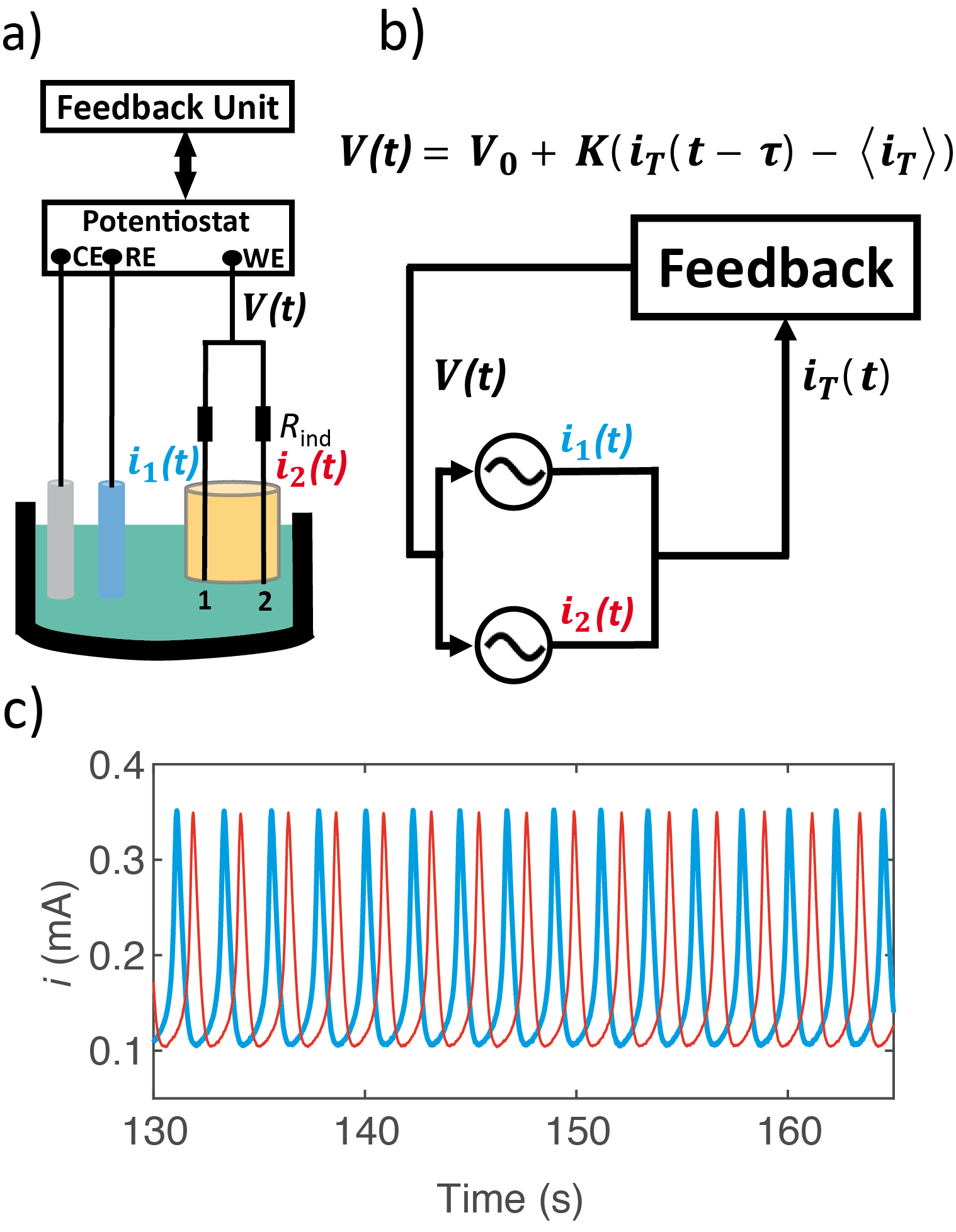
Figure 2: Illustration of the time-delayed linear feedback experiment with a time series of the uncoupled system. a) Schematic of the experimental setup. CE: Counter electrode, RE: Reference electrode, and WE: Working electrodes. b) Diagram of the delay feedback schematic of the electrochemical experiment. The currents ($i_{1}$, $i_{2}$) of each nickel wires were measured and added to obtain a total current ($i_{T}$). The $i_{T}$ was fed back with a coupling strength ($K$), a delay, ($\tau$) and applied to the circuit potential ($V(t)$). c) Time series of the currents for the uncoupled ($K=0$) oscillators and without delay ($\tau=0$). The blue and red lines correspond to oscillator 1 and 2, respectively.

A schematic of the experimental setup is shown in Figure 2a). The three-electrode electrochemical cell is equipped with a Pt coated Ti rod as a counter (C), a Hg/Hg2SO4/sat. K2SO4 as a reference (R) and two Ni wires (Goodfellow Cambridge Ltd, 99.98%, 1.0 mm diameter) as working electrodes (W) connected to a potentiostat (ACM Instruments, Gill AC). The electrodes are immersed in a $3\text{\,}\mathrm{M}$ H2SO4 solution as an electrolyte and kept at a constant temperature of $10\text{\,}\mathrm{\SIUnitSymbolCelsius}$.

When a constant circuit potential with respect to the reference electrode ($V_{0}=$1200\text{\,}\mathrm{mV}$$) is applied by the potentiostat and external resistance ($R_{\mathrm{ind}}=$1\text{\,}\mathrm{k\SIUnitSymbolOhm}$$) is attached to each nickel wire, the electrochemical dissolution of nickel exhibited periodic oscillations of the current Kiss et al. (2006) (see Figure 2c)). In our specific experiments, the natural (uncoupled) frequencies of oscillators 1 and 2 were $\omega_{1}=$0.446\text{\,}\mathrm{Hz}$$ and $\omega_{2}=$0.444\text{\,}\mathrm{Hz}$$, respectively, with a mean frequency of $0.445\text{\,}\mathrm{Hz}$ and a mean period of $T=$2.25\text{\,}\mathrm{s}$$.

The potentiostat is interfaced with a real-time LabVIEW controller, and is used to measure the total current $i_{T}$ and subsequently set the circuit potential $V(t)$ at a rate of 200 Hz according to the equation

$$V(t)=V_{0}+K(i_{T}(t-\tau)-\langle i_{T}\rangle),$$ (12)

where $V(t)$ and $V_{0}$ are the applied and the offset circuit potential, respectively, $K$ is the coupling strength, $i_{T}$ is the time averaged total current, $\langle i_{T}\rangle$ is the mean value of the total current, and $\tau$ is the time delay. The coupling between electrodes is induced using external global feedback via a small adjustment of the circuit potential according to the scheme in Figure 2b). In contrast to previous studies in which nonlinear feedback was used to couple oscillators very close to a Hopf bifurcation Rusin et al. (2010); Bick et al. (2017), the oscillators under consideration here are far from the Hopf bifurcation point, and are coupled through linear feedback. In particular, the uncoupled oscillator waveforms are far from the single harmonic profiles expected for systems close to a Hopf bifurcation. As a result, we predict that higher harmonics will be important in determining the phase dynamics as the coupling strength $K$ is increased, in line with results illustrated in Figure 1.

III.2 Results with weak coupling

We first demonstrate the system dynamics when the coupling is weak ($K=$-0.12\text{\,}\mathrm{V}\text{\,}{\mathrm{mA}}^{-1}$$) for different time-delay values. For illustration, we chose three different time-delays $\tau=$0.081\text{\,}\mathrm{s}$$, $\tau=$0.60\text{\,}\mathrm{s}$$, and $\tau=$0.89\text{\,}\mathrm{s}$$. When $\tau=$0.081\text{\,}\mathrm{s}$$, the current signal for each oscillator overlap, yielding an in-phase synchronized configuration with nearly identical peak-to-peak amplitudes ($\Delta A=A_{2}-A_{1}=$-1.0\text{\times}{10}^{-3}\text{\,}\mathrm{mA}$$, see Figure 3a)). As shown in Figure 3b), when the time delay is increased to $\tau=$0.60\text{\,}\mathrm{s}$$, an out-of-phase synchronized configuration ($\Delta\phi=4.34$ rad) is observed with a relatively large amplitude difference ($\Delta A=$-0.011\text{\,}\mathrm{mA}$$). Figure 3c) shows the dynamics when we further increased the delay to $\tau=$0.89\text{\,}\mathrm{s}$$ where we observe that the elements synchronized in an anti-phase configuration with both oscillators having similar amplitudes ($\Delta A=$-7.0\text{\times}{10}^{-4}\text{\,}\mathrm{mA}$$).

The quasi-stationary phase difference between the two coupled oscillators was experimentally measured under slow variation of $\tau$. After letting the oscillators settle to a synchronized configuration for $\tau=$0.00\text{\,}\mathrm{s}$$, measurements were taken as the time delay was slowly increased to $\tau=$1.12\text{\,}\mathrm{s}$$ ($\tau\approx T/2$; around one half period). Following this, the time delay was decreased from $\tau=$1.12\text{\,}\mathrm{s}$$ back down to $\tau=$0.00\text{\,}\mathrm{s}$$ at the same rate as the forward (increasing $\tau$) scan.

The phase difference for weak coupling strength, $K=$-0.12\text{\,}\mathrm{V}\text{\,}{\mathrm{mA}}^{-1}$$, is shown in Figure 3d). For time delays $\tau\leq 0.1T$, the oscillators exhibit a phase difference close to 0 (equivalently $2\pi$), indicating in-phase synchronization. For $0.1T<\tau\leq 0.3T$, the phase difference between the oscillators increases monotonically with respect to $\tau$ until it reached a phase difference close to $\pi$. The oscillators remain anti-phase synchronized when the time delay is further increased ($0.3T<\tau\leq 0.5T$). For decreasing $\tau$ from $\tau=0.5T$ to $\tau=0$, the system passes through a sequence of phase-locked configurations, from anti-phase, to out-of-phase, and finally to in-phase dynamics. The green and the grey lines in Figure 3d) correspond to the scan where time delay was increased and decreased, respectively, and it can be seen that the curves approximately overlap. In other words, the transition from in-phase to anti-phase through out-of-phase synchronized configurations occurs without hysteresis.

III.3 Results with strong coupling

We next investigated how the phase differences changed as $\tau$ was increased and decreased for different coupling strengths, as reported in Figure 4. When the coupling strength is weak ($K=$-0.12\text{\,}\mathrm{V}\text{\,}{\mathrm{mA}}^{-1}$$), the curves for increasing $\tau$ and for decreasing $\tau$ overlap, as observed in Figure 4a).

An increase in the coupling strength to $K=$-0.18\text{\,}\mathrm{V}\text{\,}{\mathrm{mA}}^{-1}$$ (see Figure 4b)) reveals a small region around $0.30T<\tau<0.31$ where the system possesses two stable stationary configurations coexisting simultaneously. In this case, the system exhibits bistability, and the curves for increasing and decreasing $\tau$ do not overlap. When the coupling strength increases further to $K=$-0.25\text{\,}\mathrm{V}\text{\,}{\mathrm{mA}}^{-1}$$ (see Figure 4c)), the bistability region enlarges to $0.28T<\tau<0.32T$. Finally, for $K=$-0.50\text{\,}\mathrm{V}\text{\,}{\mathrm{mA}}^{-1}$$ (see Figure 4d)), the bistability region is larger still ($0.24T<\tau<0.36T$), resulting in an extended and well-defined region where the out-of-phase and anti-phase synchronized configurations co-exist.

To better exemplify the bistable nature of the stationary configurations, we performed experiments in which the system exhibited the bistability phenomena at a strong feedback gain value $K=$-0.50\text{\,}\mathrm{V}\text{\,}{\mathrm{mA}}^{-1}$$ with appropriate initial conditions (in-phase or anti-phase) and time delay $\tau=$0.70\text{\,}\mathrm{s}$$ ($\tau=0.31T$). The time series of the current and the phase difference are shown in Figure 5a,b) for an experiment in which the system was initiated from an in-phase initial condition. After a transient time of about $25\text{\,}\mathrm{s}$, the two oscillators transition to an out-of-phase synchronized configuration with $\Delta\phi=$ 4.82 rad. Similar to the previous examples, the out-of-phase synchronized configuration has a relatively large amplitude difference, in this case, $\Delta A$ = $0.034\text{\,}\mathrm{mA}$. The corresponding experimental results starting from anti-phase initial conditions are shown in Figure 5c,d). As expected, the system remains in the anti-phase synchronized configuration with a very small amplitude difference ($\Delta A=$ $1\text{\times}{10}^{-4}\text{\,}\mathrm{mA}$).

We thus see that electrochemical oscillators display both out-of-phase and anti-phase configuration for a strong value of the coupling strength ($K=$-0.50\text{\,}\mathrm{V}\text{\,}{\mathrm{mA}}^{-1}$$) for different initial conditions, further confirming the bistability phenomena observed in the bifurcation diagram in Figure 4d). The experiments in Figure 5 also demonstrate that these configurations remained stable for at least $300\text{\,}\mathrm{s}$ (133 cycles). We next investigate whether such phenomenon can be attributed to differences in the criticality of the bifurcations of the in-phase and the anti-phase configurations.

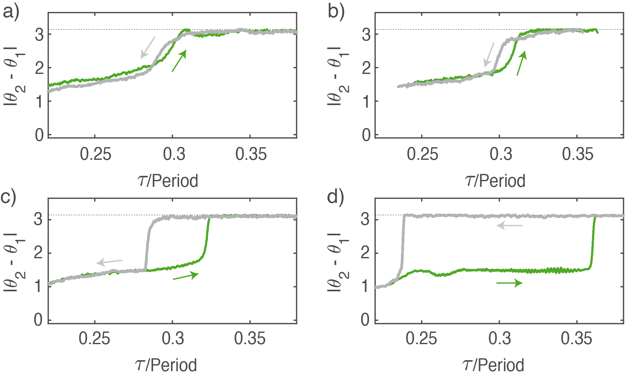
Figure 3: Scan under variation of the time delay $\tau$ at weak coupling strength ($K=$-0.12\text{\,}\mathrm{V}\text{\,}{\mathrm{mA}}^{-1}$$) of the two electrode system. a) Time series of the current for the in-phase behavior for $\tau=$0.081\text{\,}\mathrm{s}$$ (0.036 $\tau/T$). b) Time series of the current for the out-of-phase behavior for $\tau=$0.60\text{\,}\mathrm{s}$$ (0.27 $\tau/T$). c) Time series of the current for the anti-phase behavior for $\tau=$0.89\text{\,}\mathrm{s}$$ (0.39 $\tau/T$). In panels a)-c), the blue and red lines correspond to oscillators 1 and 2, respectively. d) Phase difference of the coupled oscillators as a function of the time delay. The green line is the phase difference corresponds to the forward scan ($\tau$ = 0 $\to$ 0.5 $\tau/T$), and the grey line to the backward scan ($\tau$ = 0.5 $\tau/T$ $\to$ 0) with the direction indicated by the green and grey arrows, respectively.

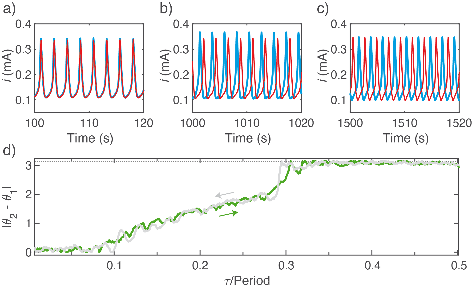
Figure 4: Phase difference under slow variation of the time delay close to the anti-phase solution for increasing coupling strengths. a) $K=$-0.12\text{\,}\mathrm{V}\text{\,}{\mathrm{mA}}^{-1}$$, b) $K=$-0.18\text{\,}\mathrm{V}\text{\,}{\mathrm{mA}}^{-1}$$, c) $K=$-0.25\text{\,}\mathrm{V}\text{\,}{\mathrm{mA}}^{-1}$$ and d) $K=$-0.50\text{\,}\mathrm{V}\text{\,}{\mathrm{mA}}^{-1}$$. The green line corresponds to the phase difference in the forward (green arrow) scan and the grey line to the backward (grey arrow) scan.

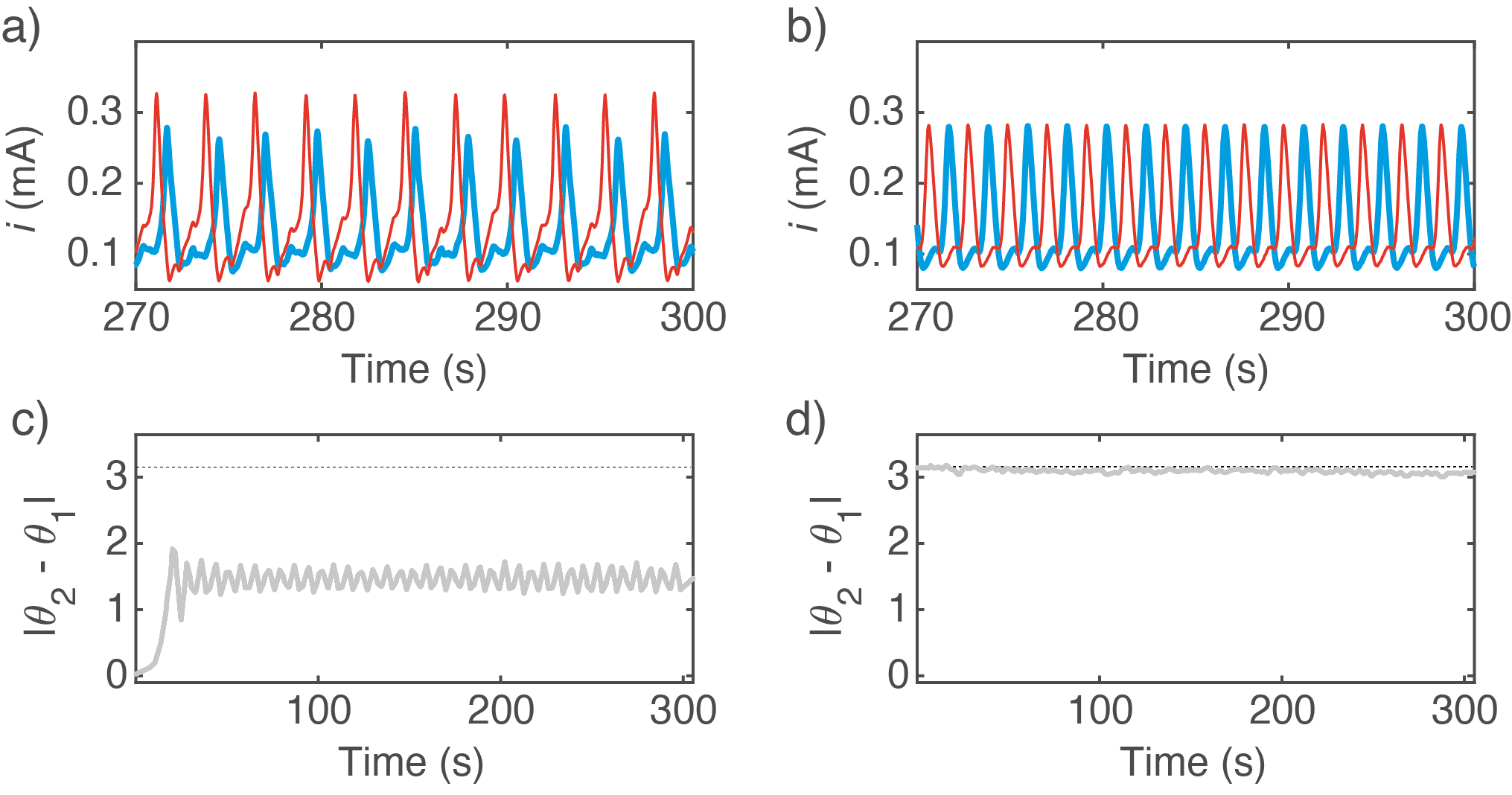
Figure 5: Time series and phase difference of the currents in the bistability region for strong feedback, $K=$-0.50\text{\,}\mathrm{V}\text{\,}{\mathrm{mA}}^{-1}$$, with time-delay $\tau=$0.70\text{\,}\mathrm{s}$$ (0.31 $\tau/T$). The panels a) and c) corresponds to the out-of-phase configuration, while panels b) and d) correspond to the anti-phase configuration. The blue and red lines correspond to oscillator 1 and 2, respectively.

IV Amplitude asymmetry in a coupled nonlinear oscillator model

The analysis of the phase model (4) in Figure 1 predicts regions in parameter space in which the pitchfork bifurcations of the in-phase and anti-phase synchronized solutions have different criticalities. In these regions, we would expect the bistability between one of these solution types and an out-of-phase solution, as observed in Figure 4. However, since the phase model disregards information about oscillation amplitude, it cannot predict the amplitude asymmetry observed in Figure 3b) and Figure 5a). Our goal in this section is to explore the qualitative asymptotic phase dynamics expected in the electrochemical experiments via bifurcation analysis of a suitable system of DDEs to further investigate this amplitude asymmetry. Some of salient synchronization features of the two electrode system have been shown to be well captured by the network Brusselator model Rusin et al. (2010):

$$\dot{x}_{i} =(B-1)x_{i}+A^{2}x_{i}+f(x_{i},y_{i})+KG(x_{j}),$$ (13a)

$$\dot{y}_{i} =-Bx_{i}-A^{2}y_{i}-f(x_{i},y_{i}),$$ (13b)

for $j\neq i$, where $i=1,2$ and

$$f(x,y)=(B/A)x^{2}+2Axy+x^{2}y.$$ (14)

We identify the $x$ component of (13) with the currents measured in the potentiostat experiments and $y$ with an unobserved recovery variable. The parameters dictating the intrinsic oscillator dynamics are hereon set to $A=0.9$ and $B=2.3$. For these parameter values and with the global coupling strength set to 0, each oscillator possesses a stable hyperbolic limit cycle with period $T=7.33$. The coupling function, which applies only to the $x$ equations of (13), is given by

$$G(x)=\sum_{n=1}^{2}k_{n}x(t-\tau_{n}-\tau)^{n}.$$ (15)

We set the amplitude ($k_{n}$) and delay ($\tau_{n}$) parameters using the synchronization engineering methods outlined in Kori et al. (2008). Briefly, we express the phase response curve of the uncoupled oscillators as a Fourier series $Z(\theta)=\sum_{n\in\mathbb{N}}Z_{n}\mathrm{e}^{in\theta}$ and a target phase interaction function as $g(\theta)=\sum_{n\in\mathbb{N}}g_{n}\mathrm{e}^{in\theta}$. The $k_{n}$ and $\tau_{n}$ parameters are then chosen so that the Fourier series representation of the coupling function, i.e., $G(\theta)=\sum_{n\in\mathbb{N}}G_{n}\mathrm{e}^{in\theta}$, are approximated by $G_{n}=Z_{n}g_{-n}$. In this study, we use a phase-shifted Hansel–Mato–Meunier type interaction function given by Hansel et al. (1993)

$$\begin{split}g(\theta)&=\sin(\theta-\tau)-r\sin(2(\theta-\tau))\\ &=-\frac{i}{2}\mathrm{e}^{i\tau}\mathrm{e}^{-i\theta}+\frac{ir}{2}\mathrm{e}^{2i\tau}\mathrm{e}^{-2i\theta}+\text{cc.},\end{split}$$ (16)

where $r$ scales the contribution of the second harmonic and $\tau$ is a common phase shift parameter. We set $r=0.5$ and consider the system dynamics under variation of $\tau$ and $K$.

For small $K$, the system dynamics is well approximated by a phase reduced model of the type given by (2) and so the phase difference $\psi$ between the two oscillators obeys (4). Since our choice for $g$ contains only two harmonics, we would not expect the pitchfork bifurcations of the in-phase and anti-phase solutions to have different criticalities for small $K$, in contrast to the predictions for the phase interaction function with three harmonics in Figure 1. In fact, it has previously been shown experimentally that phase synchronization patterns matching those expected via (4) with (16) can be achieved in the electrochemical experiment. In particular, phase locking with arbitrary steady state phase differences can be realised through variation of the common delay $\tau$ Rusin et al. (2010). Moreover, the pitchfork bifurcations of the in-phase and anti-phase synchronized solutions are both supercritical in nature and hence the system does not exhibit any bistability, unlike that observed in the experiments in Figure 4.

We use the Matlab-based package DDE-BIFTOOL to explore the asymptotic system dynamics under variation of $\tau$ as $K$ is increased. DDE-BIFTOOL is designed to perform numerical bifurcation and stability analysis of systems with fixed discrete and/or state-dependent delays. It allows for flexible encoding of systems and for the specification of additional system constraints, such as relationships between delays, which we shall leverage to implement the common delay term. The pipeline for numerical bifurcation analysis is outlined in the Appendix.

IV.1 Numerical bifurcation analysis results

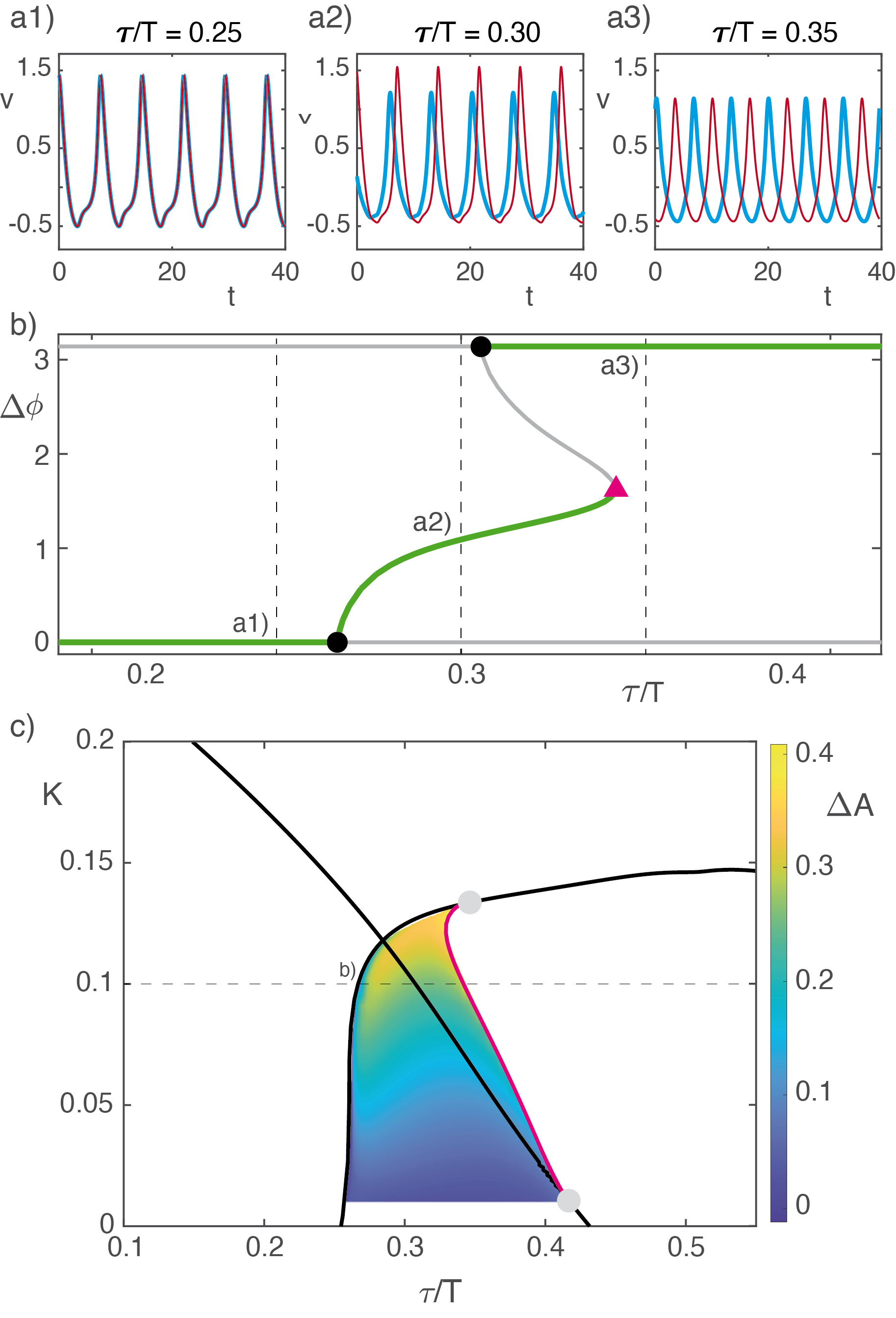
Figure 6: Bifurcation diagram and time series for the coupled Brusselator system (13) computed using DDE-BIFTOOL. a1)-a3) Time series solutions corresponding to the in-phase (a1), out-of-phase (a2) and anti-phase (a3) synchronized configurations. Blue and red lines correspond to oscillator 1 and 2, respectively. b) Bifurcation diagram under variation of $\tau$. Green and grey curves correspond to stable and unstable periodic solutions, respectively. Pitchfork bifurcations are depicted with black circles, whilst the fold of periodic orbits is marked with a pink triangle. The dashed vertical lines show where the corresponding time series in panel a) were computed. c) Two parameter bifurcation diagram under simultaneous variation of $K$ and $\tau$. The black curves correspond to pitchfork bifurcations and the pink curve represents the fold of periodic orbits. Superimposed on the diagram is a heat map showing the relative amplitude asymmetry between the oscillators along the stable part of the out-of-phase branch. The dashed horizontal line indicates where the bifurcation diagram in panel b) was computed. Bifurcations associated with changes of criticality of the pitchforks are depicted by grey markers.

The results of the bifurcation analysis procedure are shown in Figure 6. Specifically, Figure 6a) showcases temporal profiles of the $x_{i}$ along the one parameter bifurcation diagram shown in Figure 6b). These panels are to be compared with the equivalent panels in Figure 3 and Figure 4. Figure 6b) highlights the presence of unstable out-of-phase synchronized solutions along the central branch. This unstable portion of branch is generated following a change in criticality of the pitchfork bifurcation of the anti-phase solution. This can be seen more clearly in the two parameter bifurcation diagram in Figure 6c), where we observe that the pitchfork of the anti-phase solution becomes subcritical at a small positive value of $K$. This panel also shows the presence of asymmetry between the amplitudes of the two oscillators along the out-of-phase branch, just as in the experimental results shown in Figure 5a).

As $K$ increases, the amplitude asymmetry between the oscillators grows monotonically and the fold of periodics approaches the pitchfork of the in-phase solution. At $K\approx 0.14$, the two merge and the pitchfork of the in-phase solution becomes subcritical. For larger values of $K$, no stable out-of-phase solutions exist. This suggests that, for sufficiently large $K$, only the in-phase and anti-phase solutions would be observed in an experiment. However, we would still expect bistability between these solutions due to the presence of an unstable branch of out-of-phase solutions. Overall, we find that amplitude asymmetry is strongly associated with bistability of the phase-locked solutions for non-weak coupling strengths. This feature cannot be captured in the phase reduced model (2) since this approach disregards amplitude information.

V Discussion

In this article, we investigated transitions between distinct phase-locked states in a network of two delay-coupled oscillators as the coupling strength was increased, highlighting the importance of changes in the criticality of said transitions. One logical question to consider is how these results extend to networks with more oscillators. Larger networks support a greater variety of solution types, including partially synchronized cluster states Haugland et al. (2021) and chimera states in which Haugland (2021) a portion of the oscillators are phase synchronized, whilst the remaining portion are not. As such, there is a greater variety of transitions that may occur between the various states and it would informative to investigate how these how these change with respect to coupling strength. In our study, we used DDE-BIFTOOL to analyse the asymptotic solutions of the full system and show how the criticality of the bifurcations changed. A similar approach could be applied to study larger networks, however, care must to be taken when discretizing such systems to ensure that solutions remain accurate but the overall problem remains numerically tractable. Moreover, in the case of homogeneous, isotropically coupled oscillators studied here, the myriad symmetries present in larger networks can cause numerical difficulties in finding and tracking bifurcation points. In this case, additional constraints can be added to the problem structure to overcome these difficulties Krauskopf and Sieber (2023).

A more accurate low-dimensional description of the nonlinear time-delayed system can give more precise insights into the nature of the transition to in-phase or anti-phase synchronized configurations. The theoretical considerations leading to the results in Figure 1 were based on an ad-hoc phase description with a finite number of harmonics. Note that for highly nonsinusoidal oscillations—such as relaxation oscillations—a large number of harmonics is required to obtain an accurate description of the phase dynamics, even to first order in coupling strength Izhikevich (2000); Ashwin et al. (2021). Computing a phase reduction Nakao (2016); Pietras and Daffertshofer (2019) explicitly allows to link the phase parameters to the actual physical parameters in the system. Moreover, higher-order phase reductions remain valid for larger coupling strengths that we would expect in real world experimental systems. Rigorous reduction approaches for time-delayed systems are only now being developed Bick et al. (2024). Alternatively, phase-amplitude reduction that include an “amplitude” variable in addition to the phase to describe an oscillator’s state have proven useful Kotani et al. (2020); an analysis of phase-amplitude models is beyond the scope of this paper.

The existence of a phase reduction, i.e., that amplitudes are enslaved to phase variables, is not a contradiction to the asymmetry in amplitudes observed in Figure 5 and Figure 6. While traditional approaches to phase reduction have focused on deriving approximations for the phase dynamics, a recent approach based on a parametrization method von der Gracht et al. (2023) can also compute how amplitudes depend on the phases—or, in a more mathematical language, how an invariant torus is embedded in the state space of the nonlinear oscillator network. Hence, this approach can also shed light on the emergent amplitude dynamics along solutions of the phase equations.

Although our mathematical models do not aim to describe the specific electrochemical reaction in the experiment, it is still instructive to consider how well matched the features of the models and the experiment are. It is generally impossible in a real-world setting to establish perfectly identical oscillators, meaning that these systems do not possess the same symmetries as the mathematical models. However, the discrepancy we here observe is small ($<0.5\%$) and so we consider the oscillator to be approximately identical. We also cannot rule out the possibility that we observe in the experiments long-lived transient behaviour, as opposed to the asymptotic behaviour examined in our bifurcation analysis. This issue is particularly relevant for the weak coupling case in which transients may decay over long durations. To mitigate this, we varied the time delay parameter over a much slower timescale than the oscillations themselves. In addition, the abrupt transitions we observe for larger coupling strengths give us confidence that we are sufficiently well capturing asymptotic dynamics. We also note that the findings provide limitations to the extent that the synchronization engineering technique Kiss et al. (2007) can be used for tuning the phase difference between two oscillators Rusin et al. (2010). In this technique, it is assumed that the feedback gain is sufficiently strong such that the inherent natural frequency difference can be neglected. However, in this work, we showed that feedback that is too strong can induce higher order effects that impact the phase dynamics. Therefore, for oscillators with large frequency difference, techniques that take advantage of this natural frequency difference, such as phase assignment with resonant entrainment Zlotnik et al. (2016), are preferable. Overall, we expect our results to be relevant to a wide range of applications involving oscillators networks away from the weak coupling limit.

Appendix A Pipeline for numerical bifurcation analysis

The continuation of solutions with respect to a single, common delay performed in Figure 6 requires the use of DDE-BIFTOOL’s functionality to include constraints between parameters. Practically speaking, we apply a sys_cond function that fixes the difference $\tau_{1}-\tau_{2}$ to be constant and absorb this into the common delay $\tau$. Following this, we use the following pipeline:

1. Compute the isolated periodic orbit for (13) when $K=0$.

2. Set $K=\overline{K}=\Delta K=0.01$.

3. Set an initial condition for the coupled system by shifting the periodic orbit of one of the oscillators by $\alpha\in[0,\pi]$. In practice, this is done by representing the orbit by its Fourier series and then multiplying each of the Fourier coefficients by $\mathrm{e}^{-i\alpha/T}$.

4. Converge an initial periodic solution for the coupled system using a bespoke Matlab function. Repeat for the in-phase branch ($\alpha=0$), the anti-phase branch ($\alpha=\pi$), and the out-of-phase branch ($\alpha\in(0,\pi))$.

5. Continue each branch of periodic solutions over the range $\tau\in[0,T/2]$.

6. Select a point along each branch and continue said branch over the range $K\in[\overline{K},\overline{K}+\Delta K]$.

7. Increment $\overline{K}$ by $\Delta K$ and repeat steps 5-7 until the maximum value of $K$ is reached.

8. Finally, extract summary statistics along each branch, including:

   • Linear stability as determined by Floquet multipliers;

   • Phase difference, $\psi$, assessed by computing the absolute time difference between the peaks in $x_{i}$ for the two oscillators and scaling this by $2\pi/\widetilde{T}$ where $\widetilde{T}$ is the period of the periodic solution;

   • The relative amplitude asymmetry between the orbits of the two electrodes, $\Delta A=|A_{1}-A_{2}|/\min\{A_{1},A_{2}\}$, where $A_{i}=x_{i}^{\text{max}}-x_{i}^{\text{min}}$.

References

- Ashwin et al. (2016) P. Ashwin, S. Coombes, and R. Nicks, Journal of Mathematical Neuroscience 6, 1 (2016).
- Bick et al. (2020) C. Bick, M. Goodfellow, C. R. Laing, and E. A. Martens, Journal of Mathematical Neuroscience 10 (2020), 10.1186/s13408-020-00086-9.
- Filatrella et al. (2008) G. Filatrella, A. H. Nielsen, and N. F. Pedersen, European Physical Journal B 61, 485 (2008).
- Dörfler et al. (2013) F. Dörfler, M. Chertkov, and F. Bullo, Proceedings of the National Academy of Sciences of the United States of America 110, 2005 (2013), arXiv:1208.0045 .
- Yan et al. (2007) G. Yan, Z. Q. Fu, J. Ren, and W. X. Wang, Physical Review E - Statistical, Nonlinear, and Soft Matter Physics 75, 1 (2007), arXiv:0602137 [physics] .
- Gross and Kevrekidis (2008) T. Gross and I. G. Kevrekidis, Epl 82, 38004 (2008), arXiv:0702047 [nlin] .
- Hoppensteadt and Izhikevich (1997) F. C. Hoppensteadt and E. M. Izhikevich, Weakly Connected Neural Networks, Applied Mathematical Sciences No. 126 (Springer-Verlag, New York, 1997).
- Zhang et al. (2014) X. Zhang, Y. Zou, S. Boccaletti, and Z. Liu, Scientific Reports 4, 1 (2014).
- Vlasov et al. (2015) V. Vlasov, Y. Zou, and T. Pereira, Physical Review E - Statistical, Nonlinear, and Soft Matter Physics 92, 1 (2015), arXiv:1411.6873 .
- Nakao (2016) H. Nakao, Contemporary Physics 57, 188 (2016).
- Pietras and Daffertshofer (2019) B. Pietras and A. Daffertshofer, Phys Rep 819, 1 (2019).
- Kori et al. (2008) H. Kori, C. G. Rusin, I. Z. Kiss, and J. L. Hudson, Chaos 18, 026111 (2008).
- Kiss (2018) I. Z. Kiss, Current Opinion in Chemical Engineering 21, 1 (2018).
- Călugăru et al. (2020) D. Călugăru, J. F. Totz, E. A. Martens, and H. Engel, Science Advances 6, eabb2637 (2020).
- Börgers (2023) C. Börgers, Examples and Counterexamples 4, 100120 (2023).
- Guckenheimer and Worfolk (1992) J. Guckenheimer and P. Worfolk, Nonlinearity 5, 1211 (1992).
- Skardal and Arenas (2020) P. S. Skardal and A. Arenas, Communications Physics 3 (2020), 10.1038/s42005-020-00485-0, arXiv:1909.08057 .
- Bick et al. (2023) C. Bick, E. Gross, H. A. Harrington, and M. T. Schaub, SIAM Review 65, 686 (2023).
- Wedgwood et al. (2013) K. C. A. Wedgwood, K. K. Lin, R. Thul, and S. Coombes, Journal of Mathematical Neuroscience 3, 2 (2013).
- Wilson and Moehlis (2016) D. Wilson and J. Moehlis, Physical Review E 94, 052213 (2016).
- Letson and Rubin (2018) B. Letson and J. E. Rubin, SIAM Journal on Applied Dynamical Systems 17, 2414 (2018).
- Wilson and Ermentrout (2019) D. Wilson and B. Ermentrout, Physical Review Letters 123, 164101 (2019).
- Kotani et al. (2012) K. Kotani, I. Yamaguchi, Y. Ogawa, Y. Jimbo, H. Nakao, and G. B. Ermentrout, Physical Review Letters 109, 044101 (2012).
- Wilson (2020) D. Wilson, Chaos 30 (2020), 10.1063/1.5126122.
- Sakaguchi and Kuramoto (1986) H. Sakaguchi and Y. Kuramoto, Progress of Theoretical Physics 76, 576 (1986).
- Rusin et al. (2010) C. G. Rusin, H. Kori, I. Z. Kiss, and J. L. Hudson, Philos T Ro Soc A 368, 2189 (2010).
- Kuehn and Bick (2021) C. Kuehn and C. Bick, Science Advances 7, eabe3824 (2021).
- Note (1) For each parameter , we solved (4\@@italiccorr), numerically for time units with initial condition being for parameter plus a small random perturbation.
- Kiss et al. (2006) I. Z. Kiss, Z. Kazsu, and V. Gáspár, Chaos 16, 033109 (2006).
- Bick et al. (2017) C. Bick, M. Sebek, and I. Z. Kiss, Phys. Rev. Lett. 119, 168301 (2017).
- Hansel et al. (1993) D. Hansel, G. Mato, and C. Meunier, Physical Review E 48, 3470 (1993).
- Haugland et al. (2021) S. W. Haugland, A. Tosolini, and K. Krischer, Nature Communications 12 (2021), 10.1038/s41467-021-25907-7.
- Haugland (2021) S. W. Haugland, Journal of Physics: Complexity 12, 3 (2021), 10.1038/s41467-021-25907-7 .
- Krauskopf and Sieber (2023) B. Krauskopf and J. Sieber, “Bifurcation analysis of systems with delays: Methods and their use in applications,” (Springer Cham, 2023) pp. 195–245.
- Izhikevich (2000) E. M. Izhikevich, SIAM Journal on Applied Mathematics 60, 1789 (2000).
- Ashwin et al. (2021) P. Ashwin, C. Bick, and C. Poignard, Chaos 31, 093132 (2021), 2107.07152 .
- Bick et al. (2024) C. Bick, B. Rink, and B. de Wolff, “Phase reductions for delay-coupled oscillators,” (2024), In Prep.
- Kotani et al. (2020) K. Kotani, Y. Ogawa, S. Shirasaka, A. Akao, Y. Jimbo, and H. Nakao, Physical Review Research 2, 033106 (2020).
- von der Gracht et al. (2023) S. von der Gracht, E. Nijholt, and B. Rink, arXiv:2306.03320 (2023).
- Kiss et al. (2007) I. Z. Kiss, C. G. Rusin, H. Kori, and J. L. Hudson, Science 316, 1886 (2007).
- Zlotnik et al. (2016) A. Zlotnik, R. Nagao, I. Z. Kiss, and J.-S. Li, Nature Communications 7, 10788 (2016).