\setcopyright

ifaamas \acmConference[AAMAS ’24]Proc. of the 23rd International Conference on Autonomous Agents and Multiagent Systems (AAMAS 2024)May 6 – 10, 2024 Auckland, New ZealandN. Alechina, V. Dignum, M. Dastani, J.S. Sichman (eds.) \copyrightyear2024 \acmYear2024 \acmDOI \acmPrice \acmISBN \acmSubmissionID650 \affiliation \institutionShanghaitech University \cityShanghai \countryChina \affiliation \institutionShanghaiTech University \cityShanghai \countryChina \affiliation \institutionShanghaiTech University \cityShanghai \countryChina \affiliation \institutionShanghaiTech University \cityShanghai \countryChina \affiliation \institutionShanghaiTech University \cityShanghai \countryChina

Learning to Schedule Online Tasks with Bandit Feedback

Abstract.

Online task scheduling serves an integral role for task-intensive applications in cloud computing and crowdsourcing. Optimal scheduling can enhance system performance, typically measured by the reward-to-cost ratio, under some task arrival distribution. On one hand, both reward and cost are dependent on task context (e.g., evaluation metric) and remain black-box in practice. These render reward and cost hard to model thus unknown before decision making. On the other hand, task arrival behaviors remain sensitive to factors like unpredictable system fluctuation whereby a prior estimation or the conventional assumption of arrival distribution (e.g., Poisson) may fail. This implies another practical yet often neglected challenge, i.e., uncertain task arrival distribution. Towards effective scheduling under a stationary environment with various uncertainties, we propose a double-optimistic learning based Robbins-Monro (DOL-RM) algorithm. Specifically, DOL-RM integrates a learning module that incorporates optimistic estimation for reward-to-cost ratio and a decision module that utilizes the Robbins-Monro method to implicitly learn task arrival distribution while making scheduling decisions. Theoretically, DOL-RM achieves a sub-linear regret of $O(T^{3/4})$, which is the first result for online task scheduling under uncertain task arrival distribution and unknown reward and cost. Our numerical results in a synthetic experiment and a real-world application demonstrate the effectiveness of DOL-RM in achieving the best cumulative reward-to-cost ratio compared with other state-of-the-art baselines.

Key words and phrases:
Online scheduling, Double-Optimistic learning, Robbins-Monro method

1. Introduction

Refer to caption
Figure 1. Rewards and Costs for $(S,a)$ in a Toy System.
Table 1. Reward-to-Cost Ratio under Distribution $\{0.8,0.2\}$.
Algorithm Policy Ratio
The greedy algorithm $(S_{I},a_{I})$, $(S_{II},a_{III})$ 2.5
The reverse algorithm $(S_{I},a_{I})$, $(S_{II},a_{II})$ 2.6

Online task scheduling refers to the process that schedules incoming tasks to available resources in real-time. It plays a central role in boosting operational efficiency for cloud computing Agarwal and Jain (2014); Arunarani et al. (2019); Guo et al. (2012), crowdsourcing Alabbadi and Abulkhair (2021); Khazankin et al. (2011); Deng et al. (2015) and multiprocessing Drozdowski (1996); Gupta et al. (2010); Kahraman et al. (2010) systems, etc. When a task is scheduled, it occupies resources for processing, e.g., computing hardware or labor costs. Upon task completion, we receive rewards, e.g., a high-accuracy machine learning model or high-quality data. The typical goal of online task scheduling is to optimize the reward-to-cost ratio, which represents the system efficiency. For instance, a cloud computing platform bills users to process their tasks using virtualized processing units, aiming to maximize the average revenue-to-hardware cost ratio. A crowdsourcing platform compensates appropriate workers for processing data labeling tasks, aiming to optimize the quality-to-cost ratio.

There exist two major challenges to establish an effective online task scheduling policy. The first one is the black-box nature of rewards and costs. Take the machine learning model training as an example, rewards could refer to the model training accuracy, area under the curve (AUC) and f1 score while the costs could refer to the power consumption Hossin and Sulaiman (2015); Ramezani et al. (2015). The scheduler needs to choose an appropriate training time (decision) to maximize the accuracy (reward) per power consumption (cost). However, the knowledge of accuracy and power consumption w.r.t. training time is unknown apriori and thus information is only revealed for the chosen decision (i.e., bandit feedback) when the task is completed.

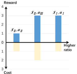
The second challenge is the uncertainty of task arrival, where there exist multiple types of tasks in the system and the scheduler has no prior information on their arrival distribution. One intuitive approach to addressing this challenge is always choosing the greedy decision with the maximal estimated ratio (suppose the knowledge of rewards and costs is known), regardless of the task type. This idea seems to work because the greedy decision for every incoming tasks would maximize the average reward-to-cost across all tasks. However, we show the greedy decision could be an arbitrarily sub-optimal solution by slightly twisting the task arrival distribution. Consider a toy task scheduling system with arriving tasks of two types in Figure 1, denoted as task $S_{I}$ and $S_{II}$. For task $S_{I}$, there is only one available decision $a_{I}$. For task $S_{II}$, two decisions exist, i.e., the first decision $a_{II}$ involves a low reward and a low cost, while the second one $a_{III}$ is characterized by a higher reward and a higher cost which has a higher reward-to-cost ratio than decision $a_{II}$. We consider two algorithms, i.e., the greedy ($a_{I}$ for task $S_{I}$ and $a_{III}$ for task $S_{II}$) and the reverse ($a_{I}$ for task $S_{I}$ and $a_{II}$ for task $S_{II}$) algorithm. One may argue that the greedy algorithm is more favorable since it achieves a higher ratio for task $S_{II}$. However, when the task arrival distribution is $\{0.8,0.2\}$ in Table 1, this intuitive algorithm achieves an expected ratio of $(0.8\times 3+0.2\times 3)/(0.8\times 1+0.2\times 2)=2.5$, which is worse than its reverse algorithm with that of $(0.8\times 3+0.2\times 1)/(0.8\times 1+0.2\times 1)=2.6$. One may then suggest to adopt the reverse algorithm instead. However, we can always construct another distribution (e.g., $\{0.2,0.8\}$) to fail the reverse algorithm such that it turns out to be worse. From this example, we emphasize the critical role of task arrival distribution in establishing effective online task scheduling algorithms.

To address the two challenges above, we propose a double-optimistic learning approach to estimate the reward and cost with bandit feedback. Intuitively, the learning approach establishes the optimistic and pessimistic estimations for rewards and costs, respectively, yielding an overall optimistic estimation for the reward-to-cost ratio. This confirms the principle, the optimism in the face of uncertainty, which is exemplified by the confidence bound based algorithms Lattimore and Szepesvári (2020). Furthermore, instead of adopting naive estimation for the task arrival distribution, we utilize the Robbins-Monro method to implicitly learn the task arrival distribution while making decisions. Intuitively, this method transforms the problem of reward-to-cost ratio maximization into a fixed point problem, which can be efficiently solved by carefully using stochastic samples and yields a fast convergence.

In summary, we propose and analyze a novel optimization framework for online task scheduling, where the objective is to optimize the cumulative reward-to-cost ratio under a stationary environment with uncertain task arrival distribution. We integrate double-optimistic learning and the Robbins-Monro method for effective and efficient online scheduling. Our main contributions are summarized as follows:

• Model for Online Task Scheduling. We propose a general framework for online task scheduling without any prior knowledge of reward, cost and task arrival distribution. This framework encapsulates a variety of practical instances whose goal is to optimize the reward-to-cost ratio, thereby striving to achieve high-return and cost-effective outcomes in real-world scheduling systems.

• Algorithm Design. We propose a novel algorithm called DOL-RM which incorporates double-optimistic learning for unknown rewards and costs and a modified Robbins-Monro method to implicitly learn the uncertain task arrival distribution. This integrated design enables the balance between rewards and costs such that the cumulative reward-to-cost ratio is maximized.

• Theoretical Analysis. We prove that DOL-RM achieves a sub-linear regret at order $O(T^{3/4})$ against the optimal scheduling policy in hindsight (Theorem 4). To prove the main result, we decompose the regret into two individual errors w.r.t. double-optimistic learning and Robbins-Monro method and then leverage the Lyapunov drift technique and carefully control the cumulative errors over the entire learning process.

• Applications. We test DOL-RM and compare it with state-of-the-art baselines via both a synthetic simulation and a real-world experiment of machine learning task scheduling. These results demonstrate that DOL-RM can achieve the best cumulative reward-to-cost ratio without any prior knowledge of reward, costs and task arrival distribution.

1.1. Related Work

Online Task Scheduling. Online task scheduling has been studied extensively in the literature. We focus on presenting the works most related to ours. In Gao et al. (2021), the authors utilize a UCB variant to address the exploration-exploitation dilemma in online task scheduling, however, the work does not take the cost into the consideration. In Li et al. (2021), a Robbins-Monro based approach is proposed for task scheduling in edge computing. However, its primary goal is to preserve data freshness, measured by Age of Information (AoI), differs from our setting of maximizing a generic reward-to-cost ratio. In Cayci et al. (2019), online bandit feedback is leveraged to schedule tasks in a renewal system, which is distinct from ours because it allows the scheduler to interrupt a task in service but the task in our model cannot be stopped once being scheduled. The closely related work is Neely (2021), which studies a similar setting with this paper except assuming the decision set and the information of reward and cost are completely known before decision making. In contrast, we focus on a more practical scenario without assuming any knowledge of the rewards and costs. Moreover, our algorithm and proof techniques are also different with Neely (2021) as we need to handle the additional uncertainties of the rewards and costs.

Cost-Aware Bandits: The key feature in our online task scheduling problem is that costs are concomitant with rewards upon decision-making. This feature is also captured in another decision-making model, i.e., the cost-aware bandit model, where an agent incurs a reward and a cost simultaneously by pulling an arm. The cost-aware bandits can be specialized into two major models, including budget-constrained bandits and the cost-aware cascading bandits. The budget-constrained bandits have been widely explored in Cayci et al. (2020); Das et al. (2022); Ding et al. (2013); Li and Xia (2017); Tran-Thanh et al. (2010, 2012); Xia et al. (2016, 2017); Zhou and Tomlin (2018), where pulling an arm incurs an additional cost and there exists a hard stopping point once the cumulative cost exceeds a given budget. Our setting has two major differences with the budget-constrained bandits. The first one is we do not have or assume any explicit budget limit constraints; and the second one is we consider a “continual” system, where it would not stop in the middle until all tasks are completed. Therefore, the previous algorithms and analysis in budget-constrained bandits cannot be applied in this paper. Besides, cost-aware cascading bandits are also related and have been studied in Cheng et al. (2022); Gan et al. (2018, 2020); Santara et al. (2022); Wang et al. (2019). Its goal is to maximize the reward-to-cost gap, however, such a maximal gap does not necessarily yield the optimal ratio as in our paper because we have multiple types of tasks in the system and need to take the task arrival distribution into consideration.

Compared to the previous works, this paper takes a bold step and investigates online task scheduling without any knowledge of rewards, costs, and task arrival distribution. Accordingly, we propose DOL-RM, an effective algorithm for optimizing the reward-to-cost ratio in online task scheduling. Furthermore, DOL-RM establishes a near-optimal regret performance for this challenging setting and has been validated to achieve the best empirical performance via a synthetic simulation and a real-world experiment.

2. System Model

We study a typical online task scheduling system where a central controller processes an incoming sequence of heterogeneous tasks in a back-to-back manner (i.e., the controller observes and processes the next task immediately upon the completion of its current task). We assume $S$ types of incoming tasks in the system, denoted by the set $\mathcal{S}\triangleq\{1,2,\cdots,S\}$ and every task is randomly drawn from a stationary probability distribution $\mathbb{P}:\mathcal{S}\to\mathbb{R}^{+}$. For the $t$th task, the controller observes its type $S_{t}\in\mathcal{S}$ and chooses a decision $a_{t}\in\mathcal{A}(S_{t}),$ where $\mathcal{A}(S_{t})$ is the corresponding available decision set of task type $S_{t}$. When the $t$th task is completed, the controller observes the feedback of reward $R_{S_{t},a_{t}}$ and cost $C_{S_{t},a_{t}},$ which are randomly generated from with the expected values $r_{S_{t},a_{t}}\triangleq\mathbb{E}[R_{S_{t},a_{t}}]$ and $c_{S_{t},a_{t}}\triangleq C_{S_{t},a_{t}}.$ Note we only observe the feedback with respect to the selected decision $a_{t},$ thus coined as “bandit feedback”, a term borrowed from bandit learning Lattimore and Szepesvári (2020). Then, the controller continues to work on the next $(t+1)$th task until $T$ tasks are completed. In the paper, we assume the rewards $\{R_{S_{t},a_{t}}\}_{t}$ and costs $\{C_{S_{t},a_{t}}\}_{t}$ are independent if $(S_{t},a_{t})$ is the same.

Refer to caption

Figure 2. Online Task Scheduling in Cloud Computing (above) and Crowdsourcing (bottom).

Reward-to-Cost Ratio Maximization: The controller aims to maximize the cumulative reward-to-cost ratio over a sequence of $T$ tasks as follows:

$$\max_{\{a_{t}\}_{t}}\frac{\sum_{t=1}^{T}\leavevmode\nobreak\ \mathbb{E}[R_{S_{t},a_{t}}]}{\sum_{t=1}^{T}\leavevmode\nobreak\ \mathbb{E}[C_{S_{t},a_{t}}]}.$$ (1)

Expectation in Problem (1) is taken over the randomness w.r.t. reward, cost and task arrival distribution $\mathbb{P}(\cdot)$. We emphasize that we do not assume any prior knowledge on such distribution and instead learn it implicitly in an online manner (please refer to Section 3).

When the task arrival distribution and the expected reward and cost are known, we can compute the optimal policy by solving Problem (1) with offline optimization techniques Fox (1966). However, such knowledge is practically unavailable or infeasible to the controller and we have to learn it by exploring the decision space in an online manner. Moreover, as discussed in the introduction, the greedy algorithm that simply maximizes ${R_{S_{t},a_{t}}}/{C_{S_{t},a_{t}}}$ for each individual task can achieve arbitrary sub-optimal performance because it ignores the task arrival distribution. Therefore, we propose an online learning based algorithm to address challenges on the uncertainties of rewards, costs and task arrivals.

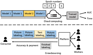
Before presenting our algorithm, we emphasize that our modeling is general to capture many real-world applications, which is illustrated with two following examples as shown in Figure 2:

  • Machine Learning (ML) model training on cloud servers: The cloud platforms (e.g., AWS, Microsoft Azure or Google Cloud) constantly process ML model training tasks submitted by users. The types of ML training tasks are unknown apriori and only revealed at the server when they are executed. For each upcoming task, the platform decides a specific training time from a range of options, which corresponds to the cost; when the training process is finished, the test accuracy is returned as the reward. However, the relationship of accuracy v.s. training time is uncertain. The goal of the platform is to schedule the training time for each individual task such that the average accuracy per time unit (i.e., accuracy-to-time ratio) is maximized.

  • Tasks assignment in Crowdsourcing: The crowdsourcing platforms (e.g., Amazon Turk or Task Rabbit) received a sequence of data labeling tasks submitted by consumers. The platform is unaware of the type of tasks until they arrive. For each task, the platform assigns it to a suitable worker from a set of candidates with various task proficiency and expertise. The quality of the labeled data from workers is considered as the reward, while his/her payment corresponds to the cost. The goal of the platform is to assign the worker for each individual task such that the average quality per dollar (i.e., quality-to-payment ratio) is maximized.

Next, we present our online learning and decision algorithm to solve the reward-to-cost ratio maximization in Problem (1).

3. Algorithm Design

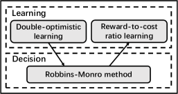
In this section, we propose a double-optimistic learning based Robbins-Monro (DOL-RM) algorithm to address the challenges induced by unknown reward, cost and task arrival distributions. Specifically, DOL-RM includes two algorithmic modules, i.e., the learning module leverages double-optimistic learning for unknown rewards and costs, and the decision module utilizes the Robbins-Monro method to make decisions via implicitly learning the task arrival distribution. As shown in Figure 3, upon each task arrives, the learning module first estimates the reward and cost via a double-optimistic learning approach. Based on the estimation, the decision module makes a proper decision through the Robbins-Monro method, which in turn provides an iteratively approaching estimation for the reward-to-cost ratio even without explicitly learning the task arrival distribution. Next, we introduce these two major modules in detail and explain the intuition behind the algorithm. The completed DOL-RM algorithm is depicted in Algorithm 1.

Refer to caption


Figure 3. Illustration of DOL-RM Algorithm.

Double-Optimistic Learning: Recall that for the $t$th task with the type $S_{t},$ the expected reward $r_{S_{t},a}$ and cost $c_{S_{t},a}$ for each decision $a\in\mathcal{A}(S_{t})$ are unknown. We consider them as multi-armed bandit problems, where each decision is regarded as an arm associated with a pair of reward and cost. Accordingly, we leverage the canonical algorithm design principle in bandit learning Lattimore and Szepesvári (2020), optimism in the face of uncertainty, to estimate the reward and cost as follows:

$\displaystyle\hat{r}_{S_{t},a}\triangleq\min\left\{r_{\max},\bar{R}_{S_{t},a}+\sqrt{\frac{\log T}{N_{S_{t},a}(t-1)}}\right\},$ (2)
$\displaystyle\check{c}_{S_{t},a}\triangleq\max\left\{c_{\min},\bar{C}_{S_{t},a}-\sqrt{\frac{\log T}{N_{S_{t},a}(t-1)}}\right\},$ (3)

where $\bar{R}_{S_{t},a}$ and $\bar{C}_{S_{t},a}$ denote the empirical means of reward and cost; $N_{S_{t},a}(t-1)$ denotes times the arm (decision) $a$ has been chosen for task of type $S_{t}$ until round $(t-1)$; $r_{\max}$ and $c_{\min}$ are the maximum reward and minimum cost, respectively. Note that $\hat{r}_{S_{t},a}$ and $\check{c}_{S_{t},a}$ denote the truncated Upper Confidence Bound (UCB) and Lower Confidence Bound (LCB) for reward and cost estimation, respectively. Recall in Problem (1), $\hat{r}_{S_{t},a}$ and $1/\check{c}_{S_{t},a}$ serve as the optimistic estimators for $\mathbb{E}[R_{S_{t},a}]$ and $1/\mathbb{E}[C_{S_{t},a}]$, yielding the name of “Double-Optimistic Learning”. Intuitively, this learning policy encourages exploration among arms (decision space) to learn the optimal reward-to-cost ratio effectively.

Suppose we make decision $a_{t}$ for the task $S_{t}$ and observe the reward $R_{S_{t},a_{t}}$ and cost $C_{S_{t},a_{t}}$ feedback when the task is completed, we conduct the following updates:

$\displaystyle N_{S_{t},a_{t}}(t)$ $\displaystyle=N_{S_{t},a_{t}}(t-1)+1,$ (4)
$\displaystyle\bar{R}_{S_{t+1},a_{t}}$ $\displaystyle=\frac{\bar{R}_{S_{t},a_{t}}N_{S_{t},a_{t}}(t-1)+R_{S_{t},a_{t}}}{N_{S_{t},a_{t}}(t)},$ (5)
$\displaystyle\bar{C}_{S_{t+1},a_{t}}$ $\displaystyle=\frac{\bar{C}_{S_{t},a_{t}}N_{S_{t},a_{t}}(t-1)+C_{S_{t},a_{t}}}{N_{S_{t},a_{t}}(t)}.$ (6)
Algorithm 1 DOL-RM
  Input: Number of tasks $T$, minimum cost $c_{\min}$, $\theta_{\max}$ and $\theta_{\min}$.
  Initialization: $\theta_{1}\leftarrow\theta_{\min}$, $\eta\leftarrow\frac{1}{c_{\min}\sqrt{T}}$.
  for $t=1,2,\dots,T$ do
     •Observation: Task type $S_{t}$ and available decision set $\mathcal{A}(S_{t})$.
     •Double-Optimistic Learning: Calculate reward and cost estimates $\hat{r}_{S_{t},a}$ and $\check{c}_{S_{t},a},\forall a\in\mathcal{A}(S_{t})$ according to (2) and (3), respectively.
     •Robbins-Monro Based Decision: Choose the greedy decision for task scheduling:
$\displaystyle a_{t}\leftarrow\underset{a\in\mathcal{A}(S_{t})}{\arg\max}\ \ \hat{r}_{S_{t},a}-\theta_{t}\ \check{c}_{S_{t},a}$ (7)
     •Bandit Feedback: Obtain reward $R_{S_{t},a_{t}}$ and cost $C_{S_{t},a_{t}}$.
     •Reward-to-Cost Ratio Learning:
$\displaystyle\theta_{t+1}\leftarrow\left[\theta_{t}+\eta(\hat{r}_{S_{t},a_{t}}-\theta_{t}\ \check{c}_{S_{t},a_{t}})\right]_{\theta_{\min}}^{\theta_{\max}}.$ (8)
Update the empirical means of rewards and costs with (4)–(6).
  end for

Robbins-Monro Based Decision: Let $\theta^{*}$ be the optimal objective (i.e., reward-to-cost ratio) in Problem (1). It is notable to observe that Problem (1) is equivalent to finding an optimal sequence of actions such that:

$$\max_{\{a_{t}\}_{t}}\leavevmode\nobreak\ \mathbb{E}\left[{\sum_{t=1}^{T}R_{S_{t},a_{t}}}-\theta^{*}{\sum_{t=1}^{T}C_{S_{t},a_{t}}}\right]=0,$$ (9)

This is essentially a fixed point problem and can be solved using the Robbins-Monro method with stochastic samples Neely (2013); Robbins and Monro (1951). Specifically, assuming the optimal ratio $\theta^{*}$ is known and using $\hat{r}_{S_{t},a}$ and $\check{c}_{S_{t},a}$ as the proxy of $R_{S_{t},a_{t}}$ and $C_{S_{t},a_{t}}$, we can follow a greedy decision for task $S_{t}\in\mathcal{S}$ according to (9):

$$\underset{a\in\mathcal{A}(S_{t})}{\arg\max}\leavevmode\nobreak\ {\hat{r}_{S_{t},a}}-\theta^{*}\ \check{c}_{S_{t},a}$$

However, this decision is non-causal and infeasible due to the lack of knowledge on the best ratio $\theta^{*}$. To learn $\theta^{*}$, we modify the Robbins-Monro iteration method by plugging the $\hat{r}_{S_{t},a}$ and $\check{c}_{S_{t},a}:$

$$\theta_{t+1}=\left[\theta_{t}+\eta(\hat{r}_{S_{t},a_{t}}-\theta_{t}\check{c}_{S_{t},a_{t}})\right]_{\theta_{\min}}^{\theta_{\max}}$$

where $\eta$ is the learning rate and $[\cdot]_{\theta_{\min}}^{\theta_{\max}}$ denotes the projection of real number onto the interval $[\theta_{\min},\theta_{\max}]$ with $\theta_{\min}\triangleq{r_{\min}}/{c_{\max}}$ and $\theta_{\max}\triangleq{r_{\max}}/{c_{\min}}$.

Note this is different with the classical RM method Robbins and Monro (1951); Neely (2021) which adopts the samples $R_{S_{t},a_{t}}$ and $C_{S_{t},a_{t}}$ for updating $\theta_{t}$. Finally, our Robbins-Monro based decision is defined as follows:

$$\underset{a\in\mathcal{A}(S_{t})}{\arg\max}\leavevmode\nobreak\ {\hat{r}_{S_{t},a}}-\theta_{t}\ \check{c}_{S_{t},a}.$$

where $\theta_{t}$ is treated as an estimation of $\theta^{*}$.

This method circumvents the need to directly estimate the task arrival distribution. Instead, it learns the optimal cumulative ratio by iteratively adjusting $\theta$ with the term $\eta(\hat{r}_{S_{t},a_{t}}-\theta_{t}\check{c}_{S_{t},a_{t}})$. When $\theta$ is excessively large, $\eta(\hat{r}_{S_{t},a_{t}}-\theta_{t}\check{c}_{S_{t},a_{t}})$ tends to be negative, driving a downward shift, whereas a small $\theta$ prompts its value to skew positive, inducing an upward adjustment in itself. With a proper learning rate $\eta$, $\theta$ can steadily converge to the optimal balance ratio as iterations increase (please refer to Section 4).

4. Theoretical Results

To present our main results, we first introduce the common assumptions on rewards and costs.

Assumption 1.

The reward $R_{S_{t},a}$ is a sub-Gaussian random variable with mean $r_{S_{t},a}=\mathbb{E}[R_{S_{t},a}]\in[r_{\min},r_{\max}]$ for any $S_{t}\in\mathcal{S},$ $a\in\mathcal{A}(S_{t})$ and $t\in[T].$

Assumption 2.

The cost $C_{S_{t},a}$ is a positive sub-Gaussian random variable with mean $c_{S_{t},a}=\mathbb{E}[C_{S_{t},a}]\in[c_{\min},c_{\max}]$ for any $S_{t}\in\mathcal{S},$ $a\in\mathcal{A}(S_{t})$ and $t\in[T].$

Regret & Convergence Gap: Let $\theta^{*}$ be the optimal reward-to-cost ratio in Problem (1), we define $Gap(T)$ to be the convergence gap:

$$Gap(T)\triangleq\left|\theta^{*}-\frac{\sum_{t=1}^{T}\mathbb{E}[R_{S_{t},a_{t}}]}{\sum_{t=1}^{T}\mathbb{E}[C_{S_{t},a_{t}}]}\right|,$$ (10)

which measures the distance between the cumulative reward-to-cost ratio returned by a policy and the optimal ratio. We define the regret to be:

$$\mathcal{R}(T)\triangleq T\cdot Gap(T).$$

Our goal is to show that DOL-RM achieves sub-linear regret $o(T)$, i.e., $\lim_{T\rightarrow\infty}\frac{\mathcal{R}(T)}{T}=\lim_{T\rightarrow\infty}Gap(T)=0$, which implies that DOL-RM converges to the optimal policy and achieves the best reward-to-cost ratio in the long-term. We state our main result for DOL-RM in the following theorem.

{theorem}

Suppose Assumption 1 and 2 hold, DOL-RM achieves the following regret:

$$\mathcal{R}(T)=O(T^{\frac{3}{4}}).$$

Theorem 4 highlights DOL-RM’s favorable theoretical performance in achieving no regret learning with sub-linear regrets $O(T^{\frac{3}{4}}),$ which implies the convergence gaps of $O(T^{-\frac{1}{4}})$. To the best of our knowledge, these are the first results for online task scheduling problems without any prior information on rewards, costs and task arrival distributions. These results also indicate that DOL-RM can quickly identify an effective and efficient policy that converges to the optimal ratio $\theta^{*}$ with the integral design of double-optimistic learning and the Robbins-Monro method.

We want to further mention two related works cited as Suttle et al. (2021) and Neely (2021). Suttle et al. (2021) studied the reward-to-cost ratio in a Markov decision process (MDP). Though MDP includes bandit as a special case, Suttle et al. (2021) only established an asymmetrical convergence. Neely (2021) assumed perfect information on the rewards and costs and established improved regrets of $O(\sqrt{T})$. With such perfect information, Neely (2021) only needs to quantify the uncertainty of task arrival without any bias111Rewards and costs are usually biased with noises, e.g., sub-Gaussian noise in our case, while Neely (2021) assumes constant rewards and costs, thus no bias involved. from rewards and costs. This enables Neely (2021) to conduct an aggressive learning scheme to control the bias only from the task arrival such that it can provide an anytime gap performance and improved performance. However, when the rewards and costs are unknown, we must carefully balance all these uncertainties and control the bias over the entire time horizon (Lemma 4.1 and 4.1), which requires a conservative learning scheme and advanced Lyapunov drift techniques to achieve sub-linear gap given coupled uncertainties.

Next, we present the detailed proof of Theorem 4 and focus on the analysis of convergence gap $Gap(T)$, where we first decompose $Gap(T)$ into the two items related to the double-optimistic learning and Robbins-Monro iteration method, respectively, and then established the items individually.

4.1. Proof of Theorem 4

Recall the definition of convergence gap in (10). We first decompose the convergence gap using triangle inequality by involving $\frac{\sum_{t=1}^{T}\mathbb{E}[\hat{r}_{S_{t},a_{t}}]}{\sum_{t=1}^{T}\mathbb{E}[\check{c}_{S_{t},a_{t}}]}$ as follows

$\displaystyle Gap(T)\leq$ $\displaystyle\underbrace{\left|\frac{\sum_{t=1}^{T}\mathbb{E}[\hat{r}_{S_{t},a_{t}}]}{\sum_{t=1}^{T}\mathbb{E}[\check{c}_{S_{t},a_{t}}]}-\frac{\sum_{t=1}^{T}\mathbb{E}[r_{S_{t},a_{t}}]}{\sum_{t=1}^{T}\mathbb{E}[c_{S_{t},a_{t}}]}\right|}_{\text{Double-optimistic learning error}}.$ (11)
$\displaystyle+\underbrace{\left|\theta^{*}-\frac{\sum_{t=1}^{T}\mathbb{E}[\hat{r}_{S_{t},a_{t}}]}{\sum_{t=1}^{T}\mathbb{E}[\check{c}_{S_{t},a_{t}}]}\right|.}_{\text{Robbins-Monro iteration convergence gap}}$ (12)

For the first term (11), we establish the bound in Lemma 4.1, which is related to the bias of optimistic learning on rewards and costs. For the second term (12), we establish the bound in Lemma 4.1 by quantifying the cumulative bias from the Robbins-Monro iteration.

Lemma \thetheorem

Suppose Assumption 1 and 2 hold, DOL-RM achieves

$$\left|\frac{\sum_{t=1}^{T}\mathbb{E}[\hat{r}_{S_{t},a_{t}}]}{\sum_{t=1}^{T}\mathbb{E}[\check{c}_{S_{t},a_{t}}]}-\frac{\sum_{t=1}^{T}\mathbb{E}[r_{S_{t},a_{t}}]}{\sum_{t=1}^{T}\mathbb{E}[c_{S_{t},a_{t}}]}\right|=O(T^{-\frac{1}{2}}).$$
Lemma \thetheorem

Suppose Assumption 1 and 2 hold, DOL-RM achieves

$$\left|\theta^{*}-\frac{\sum_{t=1}^{T}\mathbb{E}[\hat{r}_{S_{t},a_{t}}]}{\sum_{t=1}^{T}\mathbb{E}[\check{c}_{S_{t},a_{t}}]}\right|=O(T^{-\frac{1}{4}}).$$

Based on these two lemmas, we prove the convergence gap in Theorem 4 as follows:

$$Gap(T)\leq O(T^{-\frac{1}{2}})+O(T^{-\frac{1}{4}})=O(T^{-\frac{1}{4}}).$$

Here we only offer order-wise results in $O(\cdot)$ for the sake of presentation and the detailed expressions are delegated to the Appendix.

Next, we prove Lemma 4.1 and 4.1, respectively.

4.2. Double-Optimistic Learning Analysis

Lemma 4.1 represents the estimation error of the cumulative reward-to-cost ratio. Due to the page limit, we illustrate the key steps in the analysis of double-optimistic learning and the completed version can be found in Appendix C.

Recall that to optimize the reward-to-cost ratio given unknown reward and cost functions, we employ optimistic estimators for both rewards and costs. This indicates that the following inequalities hold with a high probability according to UCB/LCU learning Lattimore and Szepesvári (2020)

$$0\leq\hat{r}_{S,a}-r_{S,a}\leq 0,\leavevmode\nobreak\ 0\leq\frac{1}{\hat{c}_{S,a}}-\frac{1}{c_{S,a}}\leq 0.$$

These guarantee optimistic estimation for cumulative terms $\sum_{t=1}^{T}r_{S_{t},a_{t}}$ and $\frac{1}{\sum_{t=1}^{T}c_{S_{t},a_{t}}}$, resulting in an optimistic estimation for cumulative reward-to-cost ratio $\frac{\sum_{t=1}^{T}\mathbb{E}[r_{S_{t},a_{t}}]}{\sum_{t=1}^{T}\mathbb{E}[c_{S_{t},a_{t}}]}$.

To proceed, we define partial double-optimistic errors

$\displaystyle\epsilon(T)\triangleq$ $\displaystyle\left|\frac{\sum_{t=1}^{T}\mathbb{E}[\hat{r}_{S_{t},a_{t}}]}{\sum_{t=1}^{T}\mathbb{E}[\check{c}_{S_{t},a_{t}}]}-\frac{\sum_{t=1}^{T}\mathbb{E}[r_{S_{t},a_{t}}]}{\sum_{t=1}^{T}\mathbb{E}[\check{c}_{S_{t},a_{t}}]}\right|,$
$\displaystyle\kappa(T)\triangleq$ $\displaystyle\left|\frac{\sum_{t=1}^{T}\mathbb{E}[r_{S_{t},a_{t}}]}{\sum_{t=1}^{T}\mathbb{E}[\check{c}_{S_{t},a_{t}}]}-\frac{\sum_{t=1}^{T}\mathbb{E}[r_{S_{t},a_{t}}]}{\sum_{t=1}^{T}\mathbb{E}[c_{S_{t},a_{t}}]}\right|.$

Such errors directly form an upper bound of the double-optimistic learning error in (11) via the triangle inequality:

$$\left|\frac{\sum_{t=1}^{T}\mathbb{E}[\hat{r}_{S_{t},a_{t}}]}{\sum_{t=1}^{T}\mathbb{E}[\check{c}_{S_{t},a_{t}}]}-\frac{\sum_{t=1}^{T}\mathbb{E}[r_{S_{t},a_{t}}]}{\sum_{t=1}^{T}\mathbb{E}[c_{S_{t},a_{t}}]}\right|\leq\epsilon(T)+\kappa(T),$$

We then bound these partial double-optimistic errors as follows:

$\displaystyle\epsilon(T)+\kappa(T)$
$\displaystyle=$ $\displaystyle\frac{1}{\sum_{t=1}^{T}\mathbb{E}[\check{c}_{S_{t},a_{t}}]}\left|\sum_{t=1}^{T}\mathbb{E}[\hat{r}_{S_{t},a_{t}}]-\sum_{t=1}^{T}\mathbb{E}[r_{S_{t},a_{t}}]\right|$
$\displaystyle+\frac{\sum_{t=1}^{T}\mathbb{E}[r_{S_{t},a_{t}}]}{\sum_{t=1}^{T}\mathbb{E}[\check{c}_{S_{t},a_{t}}]\sum_{t=1}^{T}\mathbb{E}[c_{S_{t},a_{t}}]}\left|\sum_{t=1}^{T}\mathbb{E}[c_{S_{t},a_{t}}]-\sum_{t=1}^{T}\mathbb{E}[\check{c}_{S_{t},a_{t}}]\right|$
$\displaystyle\leq$ $\displaystyle\frac{1}{Tc_{\min}}\left|\sum_{t=1}^{T}\mathbb{E}[\hat{r}_{S_{t},a_{t}}-r_{S_{t},a_{t}}]\right|+\frac{r_{\max}}{Tc_{\min}^{2}}\left|\sum_{t=1}^{T}\mathbb{E}[c_{S_{t},a_{t}}-\check{c}_{S_{t},a_{t}}]\right|,$

where the last inequality holds due to the boundedness of reward and cost. As shown in the above inequality, we break down the estimated error of cumulative ratio into the estimated errors of rewards and costs. Consequently, we only need to bound the following terms

$\displaystyle\left|\sum_{t=1}^{T}\mathbb{E}[\hat{r}_{S_{t},a_{t}}-r_{S_{t},a_{t}}]\right|,\leavevmode\nobreak\ \left|\sum_{t=1}^{T}\mathbb{E}[c_{S_{t},a_{t}}-\check{c}_{S_{t},a_{t}}]\right|,$

which have been widely studied in UCB/LCB learning Lattimore and Szepesvári (2020); Liu et al. (2020, 2021) and both are in the order of $O(\sqrt{T})$. Eventually, we have

$$\epsilon(T)+\kappa(T)\leq O(T^{-\frac{1}{2}}),$$

which proves Lemma 4.1.

4.3. Robbins-Monro Iteration Analysis

Lemma 4.1 is the key to establishing the convergence gap and regret for DOL-RM and is also the most challenging part. We first establish its upper bound with the terms related to $\mathbb{E}[(\theta_{t}-\theta^{*})^{2}]$ in the following Lemma 4.3, we then carefully control the cumulative errors in the Robbins-Monro iteration.

Lemma \thetheorem

Suppose Assumption 1 and 2 hold, under DOL-RM, we bound the Robbins-Monro iteration convergence gap in (12) as follows:

$\displaystyle\left|\theta^{*}-\frac{\sum_{t=1}^{T}\mathbb{E}[\hat{r}_{S_{t},a_{t}}]}{\sum_{t=1}^{T}\mathbb{E}[\check{c}_{S_{t},a_{t}}]}\right|$
$\displaystyle\leq\max\left\{\left|\frac{\sum_{t=1}^{T}\mathbb{E}[\hat{r}_{S_{t},a_{t}}]}{\sum_{t=1}^{T}\mathbb{E}[\check{c}_{S_{t},a_{t}}]}-\frac{\sum_{t=1}^{T}\mathbb{E}[r_{S_{t},a_{t}}]}{\sum_{t=1}^{T}\mathbb{E}[c_{S_{t},a_{t}}]}\right|,\right.$ (13)
$\displaystyle\phantom{\leq\max\{}\left.\frac{\sqrt{2C_{1}}}{Tc_{\min}}\sum\limits_{t=1}^{T}\sqrt{\mathbb{E}\left[(\theta_{t}-\theta^{*})^{2}\right]}\right\}.$ (14)

We provide the proof sketch by considering two cases: 1) when $\theta^{*}\leq\frac{\sum_{t=1}^{T}\mathbb{E}[\hat{r}_{S_{t},a_{t}}]}{\sum_{t=1}^{T}\mathbb{E}[\check{c}_{S_{t},a_{t}}]}$, the term in (13) is upper bound of (12) according to the definition of $\theta^{*}$. 2) when $\frac{\sum_{t=1}^{T}\mathbb{E}[\hat{r}_{S_{t},a_{t}}]}{\sum_{t=1}^{T}\mathbb{E}[\check{c}_{S_{t},a_{t}}]}\leq\theta^{*}$, we have the greedy decision in our algorithm such that

$\displaystyle\mathbb{E}[\hat{r}_{S_{t},a_{t}}-\theta_{t}\check{c}_{S_{t},a_{t}}|\theta_{t}]\geq$ $\displaystyle\mathbb{E}[R_{S_{t},a^{*}}|\theta_{t}]-\theta_{t}\mathbb{E}[C_{S_{t},a^{*}}|\theta_{t}]$
$\displaystyle\geq$ $\displaystyle r^{*}-\theta_{t}c^{*},$

where $a^{*}$ is any decision within $\mathcal{A}(S_{t})$, the first inequality holds due to the greedy decision and $\hat{r}_{S_{t},a_{t}}\geq{r}_{S_{t},a_{t}},\check{c}_{S_{t},a_{t}}\leq c_{S_{t},a_{t}}$ holds with a high probability; the second inequality holds because $(r^{*},c^{*})$ lies within the closure of available decision set. By adding $(\theta_{t}-\theta^{*})\check{c}_{S_{t},a_{t}}$ on both sides of the above inequality, we further have

$$\mathbb{E}[\hat{r}_{S_{t},a_{t}}-\theta^{*}\check{c}_{S_{t},a_{t}}]\geq\mathbb{E}\left[(\theta_{t}-\theta^{*})(\check{c}_{S_{t},a_{t}}-c^{*})\right].$$

Finally, one could use Cauchy-Schwarz inequality to establish (14) in Lemma 4.3. More details can be found in the Appendix A.

Since we already have the $O(T^{-\frac{1}{2}})$ bound of (13) in Section 4.2, the key is to establish the cumulative error

$$\sum_{t=1}^{T}\sqrt{\mathbb{E}[(\theta_{t}-\theta^{*})^{2}]}.$$

We leverage the Lyapunov drift analysis Neely (2010); Srikant and Ying (2014) to study this key term. Note that Neely (2021) also used this technique to study the cumulative error term, where they assumed the perfect information of rewards and costs such that it can establish anytime error of $\mathbb{E}[(\theta_{t}-\theta^{*})^{2}]$ via one-step Lyapunov drift. However, we do not assume any of such knowledge and quantify the cumulative error term by aggregating the bias over all tasks.

Define the Lyapunov function

$$V_{t}\triangleq\frac{1}{2}(\theta_{t}-\theta^{*})^{2},$$

we analyze the corresponding Lyapunov drift

$$\Delta(t)\triangleq V_{t+1}-V_{t}$$

and have the following lemma.

Lemma \thetheorem

Under DOL-RM, we have the expected Lyapunov drift to be bounded as follows:

$\displaystyle\mathbb{E}[\Delta(t)]\leq$ $\displaystyle-2c_{\min}\eta\mathbb{E}[V_{t}]+\eta^{2}b$
$\displaystyle+\theta_{gap}\eta\mathbb{E}\left[\hat{r}_{S_{t},a_{t}}-r_{S_{t},a_{t}}-\theta^{*}(\check{c}_{S_{t},a_{t}}-c_{S_{t},a_{t}})\right],$

where $\theta_{gap}\triangleq(\theta_{max}-\theta_{min})$ and $b\geq\frac{1}{2}\mathbb{E}\left[(\hat{r}_{S_{t},a_{t}}-\theta_{t}\check{c}_{S_{t},a_{t}})^{2}\right],\forall t$.

We in the following provide the proof sketch for this key lemma.

According to the reward-to-cost ratio learning in (8), we have

$\displaystyle(\theta_{t+1}-\theta^{*})^{2}$ $\displaystyle=\left(\left[\theta_{t}+\eta(\hat{r}_{S_{t},a_{t}}-\theta_{t}\check{c}_{S_{t},a_{t}})\right]_{\theta_{\min}}^{\theta_{\max}}-\theta^{*}\right)^{2}$
$\displaystyle=\left[\left(\theta_{t}+\eta(\hat{r}_{S_{t},a_{t}}-\theta_{t}\check{c}_{S_{t},a_{t}})-\theta^{*}\right)_{\theta_{\min}}^{\theta_{\max}}\right]^{2}$
$\displaystyle\leq(\theta_{t}+\eta(\hat{r}_{S_{t},a_{t}}-\theta_{t}\check{c}_{S_{t},a_{t}})-\theta^{*})^{2}.$

By the definition of the Lyapunov drift $\Delta_{t}$, we have

$\displaystyle\mathbb{E}[\Delta(t)]=$ $\displaystyle\frac{1}{2}\mathbb{E}[(\theta_{t+1}-\theta^{*})^{2}]-\frac{1}{2}\mathbb{E}[(\theta_{t}-\theta^{*})^{2}]$
$\displaystyle\leq$ $\displaystyle\eta^{2}b+\eta\mathbb{E}\left[(\theta_{t}-\theta^{*})(\hat{r}_{S_{t},a_{t}}-\theta_{t}\check{c}_{S_{t},a_{t}})\right].$

Similar to the proof of Lemma 4.3, we bound the last term in the above inequality under two cases:

1) For $\theta^{*}\geq\theta_{t}$, we can directly get

$\displaystyle\mathbb{E}\left[(\theta_{t}-\theta^{*})(\hat{r}_{S_{t},a_{t}}-\theta_{t}\check{c}_{S_{t},a_{t}})\right]\leq-2c_{\min}\eta\mathbb{E}[V_{t}],$

since $\mathbb{E}[\hat{r}_{S_{t},a_{t}}-\theta_{t}\check{c}_{S_{t},a_{t}}|\theta_{t}]\geq r^{*}-\theta_{t}c^{*}=c^{*}(\theta^{*}-\theta_{t})$. Then the inequality in Lemma 4.3 holds by the fact $\mathbb{E}[\hat{r}_{S_{t},a_{t}}-r_{S_{t},a_{t}}]\geq 0,\mathbb{E}[c_{S_{t},a_{t}}-\check{c}_{S_{t},a_{t}}]\geq 0$ which is guaranteed by the property of UCB/LCB.

2) For $\theta^{*}\leq\theta_{t}$, given the boundedness of cost, we have

$\displaystyle\mathbb{E}\left[(\theta_{t}-\theta^{*})(\hat{r}_{S_{t},a_{t}}-\theta_{t}\check{c}_{S_{t},a_{t}})\right]$
\displaystyle\leq 𝔼[(θtθ)(r^St,atθcˇSt,at)]cmin𝔼[(θtθ)2].𝔼delimited-[]subscript𝜃𝑡superscript𝜃subscript^𝑟subscript𝑆𝑡subscript𝑎𝑡superscript𝜃subscriptˇ𝑐subscript𝑆𝑡subscript𝑎𝑡subscript𝑐𝑚𝑖𝑛𝔼delimited-[]superscriptsubscript𝜃𝑡superscript𝜃2\displaystyle\mathbb{E}\left[(\theta_{t}-\theta^{*})(\hat{r}_{S_{t},a_{t}}-\theta^{*}\check{c}_{S_{t},a_{t}})\right]-c_{min}\mathbb{E}\left[(\theta_{t}-\theta^{*})^{2}\right].

We then have the following bound by decomposing the first term and incorporating the fact that $\theta_{t}-\theta^{*}\leq\theta_{gap}$, i.e.,

$\displaystyle\mathbb{E}\left[(\theta_{t}-\theta^{*})(\hat{r}_{S_{t},a_{t}}-\theta^{*}\check{c}_{S_{t},a_{t}})\right]$
$\displaystyle\leq$ $\displaystyle\mathbb{E}\left[(\theta_{t}-\theta^{*})(r_{S_{t},a_{t}}-\theta^{*}c_{S_{t},a_{t}})\right]$
$\displaystyle+\theta_{gap}\mathbb{E}\left[(\hat{r}_{S_{t},a_{t}}-r_{S_{t},a_{t}}-\theta^{*}(\check{c}_{S_{t},a_{t}}-c_{S_{t},a_{t}}))\right].$

Next, drawing upon the definition of the optimal ratio $\theta^{*}$, which indicates that $\mathbb{E}\left[(r_{S_{t},a_{t}}-\theta^{*}c_{S_{t},a_{t}})\right]\leq 0,$ we complete the proof of Lemma 4.3. More details are provided in Appendix B.

Proving Lemma 4.1: We rearrange the inequality in Lemma 4.3 and take summation from $1$ to $T$ over it, yielding the following:

$\displaystyle\sum_{t=1}^{T}\mathbb{E}[V_{t}]\leq$ $\displaystyle-\sum_{t=1}^{T}\frac{\mathbb{E}[\Delta(t)]}{2c_{\min}\eta}+\frac{T\eta b}{2c_{min}}$
$\displaystyle+\frac{\theta_{gap}}{2c_{min}}\sum_{t=1}^{T}\mathbb{E}\left[\hat{r}_{S_{t},a_{t}}-r_{S_{t},a_{t}}-\theta^{*}(\check{c}_{S_{t},a_{t}}-c_{S_{t},a_{t}})\right]$
$\displaystyle\leq$ $\displaystyle\frac{V_{1}}{2c_{\min}\eta}+\frac{T\eta b}{2c_{min}}+O(\sqrt{T})=O(\sqrt{T}),$

where the second inequality holds because of $\sum_{t=1}^{T}\Delta(t)=V_{T}-V_{1}$ and the fact that the estimation errors are at the order of $O(\sqrt{T})$ according to UCB/LCB learning (similarly stated in Section 4.2); the last equality holds by plugging the learning rate $\eta=O(1/\sqrt{T})$.

According to the Cauchy-Schwarz inequality, we have,

$$\sum_{t=1}^{T}\sqrt{\mathbb{E}[V_{t}]}\leq\sqrt{T\sum_{t=1}^{T}\mathbb{E}[V_{t}]},$$

which implies that the key cumulative error is at the order of $O(T^{\frac{3}{4}})$ in the following lemma.

Lemma \thetheorem

Under DOL-RM, we have

$$\sum\limits_{t=1}^{T}\sqrt{\mathbb{E}\left[(\theta_{t}-\theta^{*})^{2}\right]}=O(T^{\frac{3}{4}}).$$

Finally, by combining Lemma 4.1 and 4.3 into Lemma 4.3, we establish the Robbins-Monro iteration convergence gap as follows:

$$\left|\theta^{*}-\frac{\sum_{t=1}^{T}\mathbb{E}[\hat{r}_{S_{t},a_{t}}]}{\sum_{t=1}^{T}\mathbb{E}[\check{c}_{S_{t},a_{t}}]}\right|\leq\max\left\{O(T^{-1/2}),O(T^{-1/4})\right\},$$

which proves Lemma 4.1.

Refer to caption
(a) Two-Task-Type $p=0.8$.
Refer to caption
(b) Two-Task-Type $p=0.6$.
Refer to caption
(c) Seven-Task-Type.
Figure 4. Synthetic Experiment: Performance Comparison in a Two-Task-Type Case and Seven-Task-Type Case.

Refer to caption

Figure 5. Real-World Experiment.

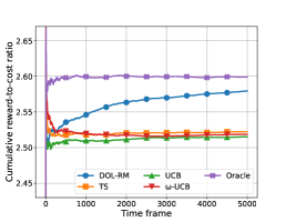
5. Numerical Results

We evaluate DOL-RM via both synthetic simulation and real-world experiment in terms of the cumulative reward-to-cost ratio $\frac{\sum_{1}^{t}R_{S_{t},a_{t}}}{\sum_{1}^{t}C_{S_{t},a_{t}}}$. For both cases, we let learning rate $\eta_{t}=1/{c_{min}(t+1)}$ in our DOL-RM algorithm.

Baselines: We consider the following representative baselines to justify DOL-RM’s performance:

  • General Thompson Sampling (TS) Russo et al. (2018).

  • Classic Upper Confidence Bound (UCB) algorithm Lattimore and Szepesvári (2020).

  • $\omega$-UCB Heyden et al. (2023), a variance-aware cost-efficient algorithm.

  • Oracle algorithm Neely (2021), which needs prior knowledge of reward and cost and an optimal solution222We adopt this algorithm as an ideal benchmark as it possesses full knowledge before decision-making, allowing us to verify whether DOL-RM converges to the optimal ratio. However, it cannot be applied in the real world due to the lack of prior knowledge..

5.1. Synthetic Simulation

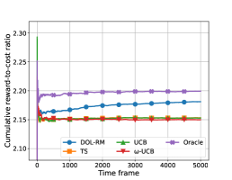
•Two-Task-Type We consider a synthetic setting similar to the toy example presented in Figure 1. We consider two incoming typs of tasks with arrival rates of $\{p,1-p\}$ and reward-cost vectors of $\{[(3,1)],[(3,2),(1,1)]\}$. The observations $R_{S,a}$ and $C_{S,a}$ are corrupted with additive Gaussian noise sampled from $\mathcal{N}(0,1)$.

We let $p$ and $1-p$ be the arrival probability of task $S_{x}$ and $S_{y}$, respectively. To verify the robustness of DOL-RM against varied task arrival distributions, we test it under two task arrival patterns, quantified by $p=0.8$, and $p=0.6$ in Figure 4(a) and  4(b).

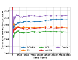
•Seven-Task-Type We consider a more complex task scheduling problem with 7 types of incoming tasks with arrival rates of $\{0.3,0.1,0.2,0.1,0.05,0.1,0.15\}$ and reward-cost vectors of $\{[(3,1)],$ $[(3,2),(1,1)],$ $[(2,1)],$ $[(2.5,1.5)],$ $[(2,1),(1,1)],$ $[(3,2),$ $(1.5,1.5)],$ $[(2.5,1)]\}$. The observations $R_{S,a}$ and $C_{S,a}$ are corrupted with additive Gaussian noise sampled from $\mathcal{N}(0,1)$.

Figure 4 demonstrates that DOL-RM outperforms the state-of-the-art learning-based algorithms in terms of the cumulative reward-to-cost ratio. DOL-RM’s superior performance is consistent across two different cases, showcasing its high adaptability. Compared to the oracle algorithm Neely (2021), which has full prior knowledge and the optimal ratio in hindsight, DOL-RM exhibits a fast convergence rate, indicating its efficiency in identifying the optimal policy under certainty.

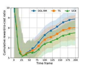
5.2. Real-World Experiment

We apply DOL-RM to schedule machine learning (ML) training tasks in a shared server. Specifically, we consider five types of ML classification tasks in the system, where a satellite image classification task $S_{s}$ with four categories , a weather classification task $S_{w}$ and a rice classification task $S_{r}$ with five categories , a natural scene classification task $S_{n}$ with six categories and a cat & dog classification task $S_{c}$. Let $\mathcal{S}=\{S_{s},S_{w},S_{r},S_{n},S_{c}\}$. For each classification task, the server decides a training epoch from a range of options. The available options on epoch number are within $\mathcal{A}(S_{s})=\mathcal{A}(S_{r})=\mathcal{A}(S_{c})=\{1,2,3,$ $4,5\}$ and $\mathcal{A}(S_{w})=\mathcal{A}(S_{n})=\{1,5,10,15,20\}$333For satellite image classification $S_{s}$, each epoch contains $141$ steps. For weather classification $S_{w}$, each epoch contains $38$ steps. For rice classification $S_{r}$, each epoch contains $100$ steps. For natural scene classification $S_{n}$, each epoch contains $150$ steps. For cat & dog classification $S_{c}$, each epoch has $30$ steps., respectively. After training the model with an epoch number $a_{t}\in\mathcal{A}(S_{t})$ for a classification task $S_{t}\in\mathcal{S}$, we can obtain the AUC on the test set as reward $R_{S_{t},a_{t}}$ and observe the training time as cost $C_{S_{t},a_{t}}$444We conduct min-max normalization on reward and cost to facilitate practical training..

The dataset of satellite image classification has more than $1000$ pictures in each category of satellite remote-sensing images  REDA (2021). All the pictures are resized into $255\times 255$ and $20\%$ of them are separated as the test set. The dataset of weather classification contains boasting over $300$ pictures of weather images in each category  GUPTA (2019). All the pictures are resized into $150\times 150$ and we construct the test set with $20\%$ of the pictures. We use the first $1000$ pictures of rice images in each class in  KOKLU (2022). The pictures are all resized into $224\times 224$ and $20\%$ of them are reserved as the test set. We take the first $500$ pictures in each category in the training set of  BANSAL (2019) as training data and utilize the test set of  BANSAL (2019) as test data. All the pictures are resized into $150\times 150$. The database of cat & dog classification contains $11875$ pictures for each class of cat or dog SACHIN (2019), where the pictures are also scaled into size $150\times 150$ and $10\%$ of these pictures are reserved as the test set. Our experiment was conducted on an RTX 3080 Ti GPU, running a 64-bit Ubuntu 18.04 system. The detailed structures and parameters of neural network models can be found in Appendix E.

Let the arrival probability of $\{S_{s},S_{w},S_{r},S_{n},S_{c}\}$ be $\{0.1,0.4,0.2,$ $0.2,0.1\}$. As $\omega$-UCB Heyden et al. (2023) and oracle algorithm Neely (2021) requires non-casual information, which is infeasible in the experiment, we compare DOL-RM only with the (classical) UCB and TS. Figure 5 plot the cumulative reward-to-cost ratio for these algorithms where the light-shaded areas indicate the corresponding standard deviation. These results show DOL-RM outperforms the baselines significantly and demonstrate that DOL-RM can converge to a better policy in the real-world system even without any prior information.

6. Conclusion

In this paper, we initiated the study on a novel formulation of the online task scheduling problem, where the task arrival distribution, rewards, and costs are all unknown. Guided by double-optimistic learning and Robbins-Monro method, we proposed an effective and efficient algorithm DOL-RM which integrates optimistic estimations and stochastic approximation of balancing point. We theoretically demonstrated its superior performance with a simultaneous achievement of sub-linear regret bound and fast learning. Via justification in synthetic and real-world scenarios, we not only showed the outperformance of DOL-RM over state-of-the-art baselines but also envisioned enormous potential applications of our modeling and algorithm design.

{acks}

The work was partly supported by the Shanghai Sailing Program 22YF1428500, the National Nature Science Foundation of China under grant 62302305. Corresponding author: Xin Liu.

References

  • (1)
  • Agarwal and Jain (2014) Dr Amit Agarwal and Saloni Jain. 2014. Efficient Optimal Algorithm of Task Scheduling in Cloud Computing Environment. International Journal of Computer Trends and Technology 9, 7 (2014), 344–349.
  • Alabbadi and Abulkhair (2021) Afra A Alabbadi and Maysoon F Abulkhair. 2021. Multi-Objective Task Scheduling Optimization in Spatial Crowdsourcing. Algorithms 14, 3 (2021), 77–97.
  • Arunarani et al. (2019) AR Arunarani, Dhanabalachandran Manjula, and Vijayan Sugumaran. 2019. Task Scheduling Techniques in Cloud Computing: A Literature Survey. Future Generation Computer Systems 91 (2019), 407–415.
  • BANSAL (2019) PUNEET BANSAL. 2019. Intel Image Classification. Retrieved December 12, 2023 from https://www.kaggle.com/datasets/puneet6060/intel-image-classification/data
  • Cayci et al. (2019) Semih Cayci, Atilla Eryilmaz, and Rayadurgam Srikant. 2019. Learning to Control Renewal Processes with Bandit Feedback. Proceedings of the ACM on Measurement and Analysis of Computing Systems 3, 2 (2019), 1–32.
  • Cayci et al. (2020) Semih Cayci, Atilla Eryilmaz, and R Srikant. 2020. Budget-Constrained Bandits over General Cost and Reward Distributions. In Proceedings of AISTATS.
  • Cheng et al. (2022) Duo Cheng, Ruiquan Huang, Cong Shen, and Jing Yang. 2022. Cascading Bandits with Two-Level Feedback. In Proceedings of IEEE ISIT.
  • Das et al. (2022) Debojit Das, Shweta Jain, and Sujit Gujar. 2022. Budgeted Combinatorial Multi-Armed Bandits. arXiv preprint arXiv:2202.03704 (2022).
  • Deng et al. (2015) Dingxiong Deng, Cyrus Shahabi, and Linhong Zhu. 2015. Task Matching and Scheduling for Multiple Workers in Spatial Crowdsourcing. In Proceedings of ACM SIGSPATIAL.
  • Ding et al. (2013) Wenkui Ding, Tao Qin, Xu-Dong Zhang, and Tie-Yan Liu. 2013. Multi-Armed Bandit with Budget Constraint and Variable Costs. In Proceedings of AAAI.
  • Drozdowski (1996) Maciej Drozdowski. 1996. Scheduling Multiprocessor Tasks: An Overview. European Journal of Operational Research 94, 2 (1996), 215–230.
  • Fox (1966) Bennett Fox. 1966. Markov Renewal Programming by Linear Fractional Programming. SIAM J. Appl. Math. 14, 6 (1966), 1418–1432.
  • Gan et al. (2018) Chao Gan, Ruida Zhou, Jing Yang, and Cong Shen. 2018. Cost-Aware Learning and Optimization for Opportunistic Spectrum Access. IEEE Transactions on Cognitive Communications and Networking 5, 1 (2018), 15–27.
  • Gan et al. (2020) Chao Gan, Ruida Zhou, Jing Yang, and Cong Shen. 2020. Cost-Aware Cascading Bandits. IEEE Transactions on Signal Processing 68 (2020), 3692–3706.
  • Gao et al. (2021) Chao Gao, Tong Mo, Taylor Zowtuk, Tanvir Sajed, Laiyuan Gong, Hanxuan Chen, Shangling Jui, and Wei Lu. 2021. Bansor: Improving Tensor Program Auto-Scheduling with Bandit Based Reinforcement Learning. In Proceedings of IEEE ICTAI.
  • Guo et al. (2012) Lizheng Guo, Shuguang Zhao, Shigen Shen, and Changyuan Jiang. 2012. Task Scheduling Optimization in Cloud Computing Based on Heuristic Algorithm. Journal of Networks 7, 3 (2012), 547–553.
  • Gupta et al. (2010) Sachi Gupta, Vikas Kumar, and Gaurav Agarwal. 2010. Task Scheduling in Multiprocessor System using Genetic Algorithm. In Proceedings of IEEE ICMLC.
  • GUPTA (2019) VIJAY GUPTA. 2019. Weather Classification. Retrieved July 13, 2023 from https://www.kaggle.com/datasets/vijaygiitk/multiclass-weather-dataset
  • Heyden et al. (2023) Marco Heyden, Vadim Arzamasov, Edouard Fouché, and Klemens Böhm. 2023. Budgeted Multi-Armed Bandits with Asymmetric Confidence Intervals. arXiv preprint arXiv:2306.07071 (2023).
  • Hossin and Sulaiman (2015) Mohammad Hossin and Md Nasir Sulaiman. 2015. A Review on Evaluation Metrics for Data Classification Evaluations. International Journal of Data Mining & Knowledge Management Process 5, 2 (2015), 01–11.
  • Kahraman et al. (2010) Cengiz Kahraman, Orhan Engin, Ihsan Kaya, and R Elif Öztürk. 2010. Multiprocessor Task Scheduling in Multistage Hybrid Flow-Shops: A Parallel Greedy Algorithm Approach. Applied Soft Computing 10, 4 (2010), 1293–1300.
  • Khazankin et al. (2011) Roman Khazankin, Harald Psaier, Daniel Schall, and Schahram Dustdar. 2011. QoS-Based Task Scheduling in Crowdsourcing Environments. In Proceedings of ICSOC.
  • KOKLU (2022) MURAT KOKLU. 2022. Rice Image Dataset. Retrieved December 12, 2023 from https://www.kaggle.com/datasets/muratkokludataset/rice-image-dataset/data
  • Lattimore and Szepesvári (2020) Tor Lattimore and Csaba Szepesvári. 2020. Bandit Algorithms. Cambridge University Press.
  • Li and Xia (2017) Haifang Li and Yingce Xia. 2017. Infinitely Many-Armed Bandits with Budget Constraints. In Proceedings of AAAI.
  • Li et al. (2021) Rui Li, Qian Ma, Jie Gong, Zhi Zhou, and Xu Chen. 2021. Age of processing: Age-Driven Status Sampling and Processing Offloading for Edge-Computing-Enabled Real-Time IoT Applications. IEEE Internet of Things Journal 8, 19 (2021), 14471–14484.
  • Liu et al. (2020) Xin Liu, Bin Li, Pengyi Shi, and Lei Ying. 2020. Pond: Pessimistic-Optimistic Online Dispatching. arXiv preprint arXiv:2010.09995 (2020).
  • Liu et al. (2021) Xin Liu, Bin Li, Pengyi Shi, and Lei Ying. 2021. An Efficient Pessimistic-Optimistic Algorithm for Stochastic Linear Bandits with General Constraints. In Advances in Neural Information Processing Systems 34 - 35th Conference on Neural Information Processing Systems, NeurIPS 2021.
  • Neely (2010) Michael J Neely. 2010. Stochastic Network Optimization with Application to Communication and Queueing Systems. Synthesis Lectures on Communication Networks 3, 1 (2010), 1–211.
  • Neely (2013) Michael J. Neely. 2013. Dynamic Optimization and Learning for Renewal Systems. IEEE Trans. Automat. Control 58, 1 (2013), 32–46.
  • Neely (2021) Michael J Neely. 2021. Fast Learning for Renewal Optimization in Online Task Scheduling. Journal of Machine Learning Research 22, 1 (2021), 12785–12828.
  • Ramezani et al. (2015) Fahimeh Ramezani, Jie Lu, Javid Taheri, and Farookh Khadeer Hussain. 2015. Evolutionary Algorithm-Based Multi-Objective Task Scheduling Optimization Model in Cloud Environments. World Wide Web 18, 6 (2015), 1737–1757.
  • REDA (2021) MAHMOUD REDA. 2021. Satellite Image Classification. Retrieved December 12, 2023 from https://www.kaggle.com/datasets/mahmoudreda55/satellite-image-classification/data
  • Robbins and Monro (1951) Herbert Robbins and Sutton Monro. 1951. A Stochastic Approximation Method. The Annals of Mathematical Statistics 22, 3 (1951), 400–407.
  • Russo et al. (2018) Daniel J Russo, Benjamin Van Roy, Abbas Kazerouni, Ian Osband, Zheng Wen, et al. 2018. A Tutorial on Thompson Sampling. Foundations and Trends® in Machine Learning 11, 1 (2018), 1–96.
  • SACHIN (2019) SACHIN. 2019. Cats-vs-Dogs. Retrieved July 15, 2023 from https://www.kaggle.com/datasets/shaunthesheep/microsoft-catsvsdogs-dataset
  • Santara et al. (2022) Anirban Santara, Gaurav Aggarwal, Shuai Li, and Claudio Gentile. 2022. Learning to Plan Variable Length Sequences of Actions with a Cascading Bandit Click Model of User Feedback. In Proceedings of AISTATS.
  • Srikant and Ying (2014) Rayadurgam Srikant and Lei Ying. 2014. Communication Networks: An Optimization, Control, and Stochastic Networks Perspective. Cambridge University Press.
  • Suttle et al. (2021) Wesley Suttle, Kaiqing Zhang, Zhuoran Yang, Ji Liu, and David Kraemer. 2021. Reinforcement Learning for Cost-Aware Markov Decision Processes. In Proceedings of ICML.
  • Tran-Thanh et al. (2010) Long Tran-Thanh, Archie Chapman, Enrique Munoz De Cote, Alex Rogers, and Nicholas R Jennings. 2010. Epsilon-First Policies for Budget-Limited Multi-Armed Bandits. In Proceedings of AAAI.
  • Tran-Thanh et al. (2012) Long Tran-Thanh, Archie Chapman, Alex Rogers, and Nicholas Jennings. 2012. Knapsack Based Optimal Policies for Budget-Limited Multi-Armed Bandits. In Proceedings of AAAI.
  • Wang et al. (2019) Chao Wang, Ruida Zhou, Jing Yang, and Cong Shen. 2019. A Cascading Bandit Approach To Efficient Mobility Management In Ultra-Dense Networks. In Proceedings of International Workshop on IEEE MLSP.
  • Xia et al. (2016) Yingce Xia, Wenkui Ding, Xu-Dong Zhang, Nenghai Yu, and Tao Qin. 2016. Budgeted Bandit Problems with Continuous Random Costs. In Proceedings of ACML.
  • Xia et al. (2017) Yingce Xia, Tao Qin, Wenkui Ding, Haifang Li, Xudong Zhang, Nenghai Yu, and Tie-Yan Liu. 2017. Finite Budget Analysis of Multi-Armed Bandit Problems. Neurocomputing 258 (2017), 13–29.
  • Zhou and Tomlin (2018) Datong Zhou and Claire Tomlin. 2018. Budget-Constrained Multi-Armed Bandits with Multiple Plays. In Proceedings of AAAI.

Appendix A Proof of Lemma 4.3

Under the case that $\theta^{*}\leq\frac{\sum_{t=1}^{T}\mathbb{E}[\hat{r}_{S_{t},a_{t}}]}{\sum_{t=1}^{T}\mathbb{E}[\check{c}_{S_{t},a_{t}}]}$, the following inequality holds obviously,

$$\left|\theta^{*}-\frac{\sum_{t=1}^{T}\mathbb{E}[\hat{r}_{S_{t},a_{t}}]}{\sum_{t=1}^{T}\mathbb{E}[\check{c}_{S_{t},a_{t}}]}\right|\leq\left|\frac{\sum_{t=1}^{T}\mathbb{E}[\hat{r}_{S_{t},a_{t}}]}{\sum_{t=1}^{T}\mathbb{E}[\check{c}_{S_{t},a_{t}}]}-\frac{\sum_{t=1}^{T}\mathbb{E}[r_{S_{t},a_{t}}]}{\sum_{t=1}^{T}\mathbb{E}[c_{S_{t},a_{t}}]}\right|,$$

We then focus on the case that $\theta^{*}\geq\frac{\sum_{t=1}^{T}\mathbb{E}[\hat{r}_{S_{t},a_{t}}]}{\sum_{t=1}^{T}\mathbb{E}[\check{c}_{S_{t},a_{t}}]}$, and we start with the following lemma.

Lemma \thetheorem (Lemma $3$ in Neely (2021))

Under DOL-RM, the following inequalities hold for all $t\in[T]$:

$$\mathbb{E}[\hat{r}_{S_{t},a_{t}}-\theta^{*}\check{c}_{S_{t},a_{t}}|\theta_{t}]\geq(\theta_{t}-\theta^{*})\mathbb{E}[\check{c}_{S_{t},a_{t}}-c^{*}|\theta_{t}].$$
Proof.

According to the updating rule of $a_{t}$ in (7), we have

$$\hat{r}_{S_{t},a_{t}}-\theta_{t}\check{c}_{S_{t},a_{t}}\geq\hat{r}_{S_{t},a}-\theta_{t}\check{c}_{S_{t},a},\leavevmode\nobreak\ \forall a\in\mathcal{A}(S_{t}).$$

Take conditional expectations at both sides and we get,

$$\mathbb{E}[\hat{r}_{S_{t},a_{t}}-\theta_{t}\check{c}_{S_{t},a_{t}}|\theta_{t}]\geq\mathbb{E}[\hat{r}_{S_{t},a}|\theta_{t}]-\theta_{t}\mathbb{E}[\check{c}_{S_{t},a}|\theta_{t}].$$ (15)

Since $\hat{r}_{S_{t},a}$ and $\check{c}_{S_{t},a}$ serve as optimistic UCB/LCB estimators, the following inequalities hold with probability $1$,

$$\mathbb{E}[\check{c}_{S_{t},a}|\theta_{t}]\leq\mathbb{E}[C_{S_{t},a}|\theta_{t}],\leavevmode\nobreak\ \mathbb{E}[\hat{r}_{S_{t},a}|\theta_{t}]\geq\mathbb{E}[R_{S_{t},a}|\theta_{t}].$$ (16)

Substituting (16) into (15) yields

$$\mathbb{E}[\hat{r}_{S_{t},a_{t}}-\theta_{t}\check{c}_{S_{t},a_{t}}|\theta_{t}]\geq\mathbb{E}[R_{S_{t},a}|\theta_{t}]-\theta_{t}\mathbb{E}[C_{S_{t},a}|\theta_{t}].$$

Since $\theta_{t}$ only depends on the history in the system before $t$, it is independent of $S_{t}$. Fix $(r,c)\in\mathcal{D}$, where $\mathcal{D}$ represents the set of all reward-cost pairs corresponding to all available decisions. There is a conditional distribution for choosing $(R_{S_{1},a_{1}},C_{S_{1},a_{1}})\in\mathcal{D}(S_{1})$, given the observed $S_{1}$, such that $(\mathbb{E}[r_{S_{1},a_{1}}],\mathbb{E}[c_{S_{1},a_{1}}])=(r,c)$. Since $S_{t}$ is independent of $\theta_{t}$ and has the same distribution as $S_{1}$, we can use the same conditional distribution to get a result of a bandit $(r_{S_{t},a^{*}},c_{S_{t},a^{*}})\in\mathcal{D}(S_{t})$ that is independent of $\theta_{t}$ such that

$$(\mathbb{E}[R_{S_{t},a^{*}}],\mathbb{E}[C_{S_{t},a^{*}}])=(r,c).$$

Besides, since $(\mathbb{E}[R_{S_{t},a^{*}}],\mathbb{E}[C_{S_{t},a^{*}}])$ is independent of $\theta_{t}$, we have (with probability 1)

$$\mathbb{E}[R_{S_{t},a^{*}}|\theta_{t}]=r,\leavevmode\nobreak\ \mathbb{E}[C_{S_{t},a^{*}}|\theta_{t}]=c,$$

which indicates that

$$\mathbb{E}[\hat{r}_{S_{t},a_{t}}-\theta_{t}\check{c}_{S_{t},a_{t}}|\theta_{t}]\geq r-\theta_{t}c.$$ (17)

Fix $(r^{*},c^{*})\in\bar{\mathcal{D}}$ that satisfies $\theta^{*}=\frac{r^{*}}{c^{*}}$. Since $\bar{\mathcal{D}}$ is the closure of the set $\mathcal{D}$, there is a sequence of points $\{(r_{i},c_{i})\}_{i=1}^{\infty}$ in $\mathcal{D}$ that converge to the value $(r^{*},c^{*})$. Since (17) holds for an arbitrary $(r,c)\in\mathcal{D}$, with probability 1, it holds simultaneously for all of $(r_{i},c_{i})\in\mathcal{D}$ for $i\in\{1,2,\dots\}$. Therefore, we have

$$\mathbb{E}[\hat{r}_{S_{t},a_{t}}-\theta_{t}\check{c}_{S_{t},a_{t}}|\theta_{t}]\geq r_{i}-\theta_{t}c_{i}.$$

Taking a limit as $i\rightarrow\infty$ yields (with probability 1):

$$\mathbb{E}[\hat{r}_{S_{t},a_{t}}-\theta_{t}\check{c}_{S_{t},a_{t}}|\theta_{t}]\geq r^{*}-\theta_{t}c^{*}=c^{*}(\theta^{*}-\theta_{t}).$$ (18)

Adding $(\theta_{t}-\theta^{*})\mathbb{E}[\check{c}_{S_{t},a_{t}}|\theta_{t}]$ to both sides implies:

$$\mathbb{E}[\hat{r}_{S_{t},a_{t}}-\theta^{*}\check{c}_{S_{t},a_{t}}|\theta_{t}]\geq(\theta^{*}-\theta_{t})c^{*}+(\theta_{t}-\theta^{*})\mathbb{E}[\check{c}_{S_{t},a_{t}}|\theta_{t}].$$

Taking expectations on both sides, we have

$$\mathbb{E}[\hat{r}_{S_{t},a_{t}}-\theta^{*}\check{c}_{S_{t},a_{t}}|\theta_{t}]\geq\mathbb{E}\left[(\theta_{t}-\theta^{*})(\check{c}_{S_{t},a_{t}}-c^{*})|\theta_{t}\right].$$

Takning expectation on both sides of the above inequality, we have

$\displaystyle\mathbb{E}[\hat{r}_{S_{t},a_{t}}-\theta^{*}\check{c}_{S_{t},a_{t}}]\geq\mathbb{E}\left[(\theta_{t}-\theta^{*})(\check{c}_{S_{t},a_{t}}-c^{*})\right].$

Take summation and rearrange the above inequality, we have

$\displaystyle\frac{\sum_{t=1}^{T}\mathbb{E}[\hat{r}_{S_{t},a_{t}}]}{\sum_{t=1}^{T}\mathbb{E}[\check{c}_{S_{t},a_{t}}]}$ $\displaystyle\geq\theta^{*}+\frac{1}{{\sum_{t=1}^{T}\mathbb{E}[\check{c}_{S_{t},a_{t}}]}}\sum_{t=1}^{T}\mathbb{E}\left[(\theta_{t}-\theta^{*})(\check{c}_{S_{t},a_{t}}-c^{*})\right]$
$\displaystyle\geq\theta^{*}-\frac{1}{Tc_{\min}}\sum_{t=1}^{T}\mathbb{E}[|\theta_{t}-\theta^{*}||\check{c}_{S_{t},a_{t}}-c^{*}|],$

where the last inequality comes from the truncation of $\check{c}_{S_{t},a_{t}}$. According to the condition $\theta^{*}\geq\frac{\sum_{t=1}^{T}\mathbb{E}[\hat{r}_{S_{t},a_{t}}]}{\sum_{t=1}^{T}\mathbb{E}[\check{c}_{S_{t},a_{t}}]}$, we prove the following inequality which completes the proof of Lemma 4.3,

$\displaystyle\left|\theta^{*}-\frac{\sum_{t=1}^{T}\mathbb{E}[\hat{r}_{S_{t},a_{t}}]}{\sum_{t=1}^{T}\mathbb{E}[\check{c}_{S_{t},a_{t}}]}\right|$ $\displaystyle=\theta^{*}-\frac{\sum_{t=1}^{T}\mathbb{E}[\hat{r}_{S_{t},a_{t}}]}{\sum_{t=1}^{T}\mathbb{E}[\check{c}_{S_{t},a_{t}}]}$
$\displaystyle\leq\frac{1}{Tc_{\min}}\sum_{t=1}^{T}\mathbb{E}[|\theta_{t}-\theta^{*}||\check{c}_{S_{t},a_{t}}-c^{*}|]$ (19)
$\displaystyle\overset{(a)}{\leq}\frac{1}{Tc_{\min}}\sum_{t=1}^{T}\sqrt{\mathbb{E}\left[(\theta_{t}-\theta^{*})^{2}(\check{c}_{S_{t},a_{t}}-c^{*})^{2}\right]}$ (20)
$\displaystyle\overset{(b)}{\leq}\frac{\sqrt{2C_{1}}}{Tc_{\min}}\sum\limits_{t=1}^{T}\sqrt{\mathbb{E}\left[(\theta_{t}-\theta^{*})^{2}\right]},$ (21)

where $(a)$ follows by the Cauchy-Schwarz inequality; $(b)$ holds because $(\check{c}_{S_{t},a_{t}}-c^{*})^{2}\leq\check{c}_{S_{t},a_{t}}^{2}+(c^{*})^{2}\leq 2C_{1}^{2}$ with $(C_{1}\geq\mathbb{E}[c_{S,a}^{2}],\leavevmode\nobreak\ \forall a\in\mathcal{A}(S))$.

Appendix B Proof of Lemma 4.3

According to virtual queue update of $\theta_{t}$ in (8), we have

$\displaystyle(\theta_{t+1}-\theta^{*})^{2}$ $\displaystyle=\left(\left[\theta_{t}+\eta(\hat{r}_{S_{t},a_{t}}-\theta_{t}\check{c}_{S_{t},a_{t}})\right]_{\theta_{\min}}^{\theta_{\max}}-\theta^{*}\right)^{2}$
$\displaystyle=\left(\left[\theta_{t}+\eta(\hat{r}_{S_{t},a_{t}}-\theta_{t}\check{c}_{S_{t},a_{t}})\right]_{\theta_{\min}}^{\theta_{\max}}-[\theta^{*}]_{\theta_{\min}}^{\theta_{\max}}\right)^{2}$
$\displaystyle=\left[\left(\theta_{t}+\eta(\hat{r}_{S_{t},a_{t}}-\theta_{t}\check{c}_{S_{t},a_{t}})-\theta^{*}\right)_{\theta_{\min}}^{\theta_{\max}}\right]^{2}$
$\displaystyle\leq(\theta_{t}+\eta(\hat{r}_{S_{t},a_{t}}-\theta_{t}\check{c}_{S_{t},a_{t}})-\theta^{*})^{2}.$

Recall the definition $V_{t}=\frac{1}{2}(\theta_{t}-\theta^{*})^{2}$, we have

$\displaystyle V_{t+1}$ $\displaystyle\leq\frac{1}{2}((\theta_{t}-\theta^{*})+\eta(\hat{r}_{S_{t},a_{t}}-\theta_{t}\check{c}_{S_{t},a_{t}}))^{2}$
$\displaystyle=V_{t}+\frac{\eta^{2}}{2}(\hat{r}_{S_{t},a_{t}}-\theta_{t}\check{c}_{S_{t},a_{t}})^{2}+\eta(\theta_{t}-\theta^{*})(\hat{r}_{S_{t},a_{t}}-\theta_{t}\check{c}_{S_{t},a_{t}}).$

Taking expectations on both sides, we have

$$\mathbb{E}\left[V_{t+1}\right]\leq\mathbb{E}\left[V_{t}\right]+\eta^{2}b+\eta\mathbb{E}\left[(\theta_{t}-\theta^{*})(\hat{r}_{S_{t},a_{t}}-\theta_{t}\check{c}_{S_{t},a_{t}})\right],$$

where $b\geq\frac{1}{2}\mathbb{E}\left[(\hat{r}_{S_{t},a_{t}}-\theta_{t}\check{c}_{S_{t},a_{t}})^{2}\right],\forall t$.

To prove Lemma 4.3, it suffices to show

$$\mathbb{E}\left[(\theta_{t}-\theta^{*})(\hat{r}_{S_{t},a_{t}}-\theta_{t}\check{c}_{S_{t},a_{t}})\right]\leq-c_{\min}\mathbb{E}\left[(\theta_{t}-\theta^{*})^{2}\right]+\theta_{gap}\mathbb{E}\left[\hat{r}_{S_{t},a_{t}}-r_{S_{t},a_{t}}-\theta^{*}(\check{c}_{S_{t},a_{t}}-c_{S_{t},a_{t}})\right].$$

We consider the proof under two cases separately:

  • When $\theta_{t}-\theta^{*}<0$, take expectation of (18) we can straightly get

    $\displaystyle\mathbb{E}\left[(\theta_{t}-\theta^{*})(\hat{r}_{S_{t},a_{t}}-\theta_{t}\check{c}_{S_{t},a_{t}})\right]$ $\displaystyle\leq-c^{*}\mathbb{E}\left[(\theta_{t}-\theta^{*})^{2}\right]$
    $\displaystyle\leq-c_{\min}\mathbb{E}\left[(\theta_{t}-\theta^{*})^{2}\right]+\theta_{gap}\mathbb{E}\left[\hat{r}_{S_{t},a_{t}}-r_{S_{t},a_{t}}-\theta^{*}(\check{c}_{S_{t},a_{t}}-c_{S_{t},a_{t}})\right],$

    where the last inequality holds since $c^{*}\geq c_{\min}$ and $\mathbb{E}\left[\hat{r}_{S_{t},a_{t}}-r_{S_{t},a_{t}}-\theta^{*}(\check{c}_{S_{t},a_{t}}-c_{S_{t},a_{t}})\right]\geq 0$.

  • When $\theta_{t}-\theta^{*}\geq 0$, given the boundedness of cost:

    $\displaystyle\mathbb{E}\left[(\theta_{t}-\theta^{*})(\hat{r}_{S_{t},a_{t}}-\theta_{t}\check{c}_{S_{t},a_{t}})\right]=$ $\displaystyle\mathbb{E}\left[(\theta_{t}-\theta^{*})(\hat{r}_{S_{t},a_{t}}-\theta^{*}\check{c}_{S_{t},a_{t}})\right]-\check{c}_{S_{t},a_{t}}\mathbb{E}\left[(\theta_{t}-\theta^{*})^{2}\right]$
    \displaystyle\leq 𝔼[(θtθ)(r^St,atθcˇSt,at)]cmin𝔼[(θtθ)2].𝔼delimited-[]subscript𝜃𝑡superscript𝜃subscript^𝑟subscript𝑆𝑡subscript𝑎𝑡superscript𝜃subscriptˇ𝑐subscript𝑆𝑡subscript𝑎𝑡subscript𝑐𝑚𝑖𝑛𝔼delimited-[]superscriptsubscript𝜃𝑡superscript𝜃2\displaystyle\mathbb{E}\left[(\theta_{t}-\theta^{*})(\hat{r}_{S_{t},a_{t}}-\theta^{*}\check{c}_{S_{t},a_{t}})\right]-c_{min}\mathbb{E}\left[(\theta_{t}-\theta^{*})^{2}\right].

    For the first term, we have

    $\displaystyle\mathbb{E}\left[(\theta_{t}-\theta^{*})(\hat{r}_{S_{t},a_{t}}-\theta^{*}\check{c}_{S_{t},a_{t}})\right]=$ $\displaystyle\mathbb{E}\left[(\theta_{t}-\theta^{*})(r_{S_{t},a_{t}}-\theta^{*}c_{S_{t},a_{t}})\right]+\mathbb{E}\left[(\theta_{t}-\theta^{*})(\hat{r}_{S_{t},a_{t}}-r_{S_{t},a_{t}}-\theta^{*}(\check{c}_{S_{t},a_{t}}-c_{S_{t},a_{t}}))\right].$
    $\displaystyle\leq\mathbb{E}\left[(\theta_{t}-\theta^{*})(r_{S_{t},a_{t}}-\theta^{*}c_{S_{t},a_{t}})\right]+\theta_{gap}\mathbb{E}\left[(\hat{r}_{S_{t},a_{t}}-r_{S_{t},a_{t}}-\theta^{*}(\check{c}_{S_{t},a_{t}}-c_{S_{t},a_{t}}))\right].$

    Recall the definition of optimal ratio $\theta^{*}$, we can get

    $$\mathbb{E}[r_{S_{t},a_{t}}|\theta_{t}]-\theta^{*}\mathbb{E}[c_{S_{t},a_{t}}|\theta_{t}]\leq\sup\limits_{(r,c)\in\bar{\mathcal{D}}}\{r-\theta^{*}c\}=0,$$

    which indicates that

    $$\mathbb{E}\left[(\theta_{t}-\theta^{*})(r_{S_{t},a_{t}}-\theta^{*}c_{S_{t},a_{t}})\right]\leq 0.$$

    Combine these inequalities and we complete the proof as follows:

    $\displaystyle\mathbb{E}\left[(\theta_{t}-\theta^{*})(\hat{r}_{S_{t},a_{t}}-\theta_{t}\check{c}_{S_{t},a_{t}})\right]\leq-c_{\min}\mathbb{E}\left[(\theta_{t}-\theta^{*})^{2}\right]+\theta_{gap}\mathbb{E}\left[\hat{r}_{S_{t},a_{t}}-r_{S_{t},a_{t}}-\theta^{*}(\check{c}_{S_{t},a_{t}}-c_{S_{t},a_{t}})\right].$

Appendix C Proof of Lemma 4.1

Applying the triangle inequality on (13), we have

$\displaystyle\left|\frac{\sum_{t=1}^{T}\mathbb{E}[\hat{r}_{S_{t},a_{t}}]}{\sum_{t=1}^{T}\mathbb{E}[\check{c}_{S_{t},a_{t}}]}-\frac{\sum_{t=1}^{T}\mathbb{E}[r_{S_{t},a_{t}}]}{\sum_{t=1}^{T}\mathbb{E}[c_{S_{t},a_{t}}]}\right|$
$\displaystyle\leq$ $\displaystyle\left|\frac{\sum_{t=1}^{T}\mathbb{E}[\hat{r}_{S_{t},a_{t}}]}{\sum_{t=1}^{T}\mathbb{E}[\check{c}_{S_{t},a_{t}}]}-\frac{\sum_{t=1}^{T}\mathbb{E}[r_{S_{t},a_{t}}]}{\sum_{t=1}^{T}\mathbb{E}[\check{c}_{S_{t},a_{t}}]}\right|+\left|\frac{\sum_{t=1}^{T}\mathbb{E}[r_{S_{t},a_{t}}]}{\sum_{t=1}^{T}\mathbb{E}[\check{c}_{S_{t},a_{t}}]}-\frac{\sum_{t=1}^{T}\mathbb{E}[r_{S_{t},a_{t}}]}{\sum_{t=1}^{T}\mathbb{E}[c_{S_{t},a_{t}}]}\right|$
$\displaystyle=$ $\displaystyle\frac{1}{\sum_{t=1}^{T}\mathbb{E}[\check{c}_{S_{t},a_{t}}]}\left|\sum_{t=1}^{T}\mathbb{E}[\hat{r}_{S_{t},a_{t}}]-\sum_{t=1}^{T}\mathbb{E}[r_{S_{t},a_{t}}]\right|+\frac{\sum_{t=1}^{T}\mathbb{E}[r_{S_{t},a_{t}}]}{\sum_{t=1}^{T}\mathbb{E}[\check{c}_{S_{t},a_{t}}]\sum_{t=1}^{T}\mathbb{E}[c_{S_{t},a_{t}}]}\left|\sum_{t=1}^{T}\mathbb{E}[c_{S_{t},a_{t}}]-\sum_{t=1}^{T}\mathbb{E}[\check{c}_{S_{t},a_{t}}]\right|$
$\displaystyle\leq$ $\displaystyle\frac{1}{Tc_{\min}}|\sum_{t=1}^{T}\mathbb{E}[\hat{r}_{S_{t},a_{t}}]-\sum_{t=1}^{T}\mathbb{E}[r_{S_{t},a_{t}}]|+\frac{r_{\max}}{Tc_{\min}^{2}}|\sum_{t=1}^{T}\mathbb{E}[c_{S_{t},a_{t}}]-\sum_{t=1}^{T}\mathbb{E}[\check{c}_{S_{t},a_{t}}]|,$

where the last inequality comes from the boundedness of cost and reward. This inequality breaks down the cumulative ratio estimate error into the estimated errors of reward and cost. Consequently, we only need to bound the following terms:

$$\left|\sum_{t=1}^{T}\mathbb{E}[\hat{r}_{S_{t},a_{t}}]-\sum_{t=1}^{T}\mathbb{E}[r_{S_{t},a_{t}}]\right|,\leavevmode\nobreak\ \left|\sum_{t=1}^{T}\mathbb{E}[c_{S_{t},a_{t}}]-\sum_{t=1}^{T}\mathbb{E}[\check{c}_{S_{t},a_{t}}]\right|,$$

which have been widely studied in UCB/LCB learning Lattimore and Szepesvári (2020); Liu et al. (2020).

We first prove the error bound for reward function $r$ and the analysis of cost function $c$ follows the same steps. Define $x_{S_{t},a}$ as the probability that arm $a\in\mathcal{A}(S_{t})$ is pulled at time frame $t$ and we have

$\displaystyle\left|\sum_{t=1}^{T}\mathbb{E}[\hat{r}_{S_{t},a_{t}}]-\sum_{t=1}^{T}\mathbb{E}[r_{S_{t},a_{t}}]\right|=$ $\displaystyle\sum_{t=1}^{T}\sum_{a\in\mathcal{A}(S_{t})}\mathbb{E}\left[(\hat{r}_{S_{t},a}-r_{S_{t},a})x_{S_{t},a}\right]$
$\displaystyle=$ $\displaystyle\sum_{a\in\mathcal{A}(S_{t})}\left[\sum_{t=1}^{T}\mathbb{E}\left[(\hat{r}_{S_{t},a}-r_{S_{t},a})\mathbb{I}(\hat{r}_{S_{t},a}-r_{S_{t},a}\leq\zeta)x_{S_{t},a}\right]+\mathbb{E}\left[(\hat{r}_{S_{t},a}-r_{S_{t},a})\mathbb{I}(\hat{r}_{S_{t},a}-r_{S_{t},a}>\zeta)x_{S_{t},a}\right]\right]$
$\displaystyle\leq$ $\displaystyle T\zeta\sum_{a\in\mathcal{A}(S_{t})}\mathbb{E}[x_{S_{t},a}]+\sum_{a\in\mathcal{A}(S_{t})}\sum_{t=1}^{T}\mathbb{E}\left[(\hat{r}_{S_{t},a}-r_{S_{t},a})\mathbb{I}(\hat{r}_{S_{t},a}-r_{S_{t},a}>\zeta)x_{S_{t},a}\right]$
$\displaystyle\overset{(a)}{\leq}$ $\displaystyle T\zeta+\sum_{a\in\mathcal{A}(S_{t})}\int_{\zeta}^{\infty}\sum_{t=1}^{T}\mathbb{P}(\hat{r}_{S_{t},a}-r_{S_{t},a}>y)dy$
$\displaystyle\overset{(b)}{=}$ $\displaystyle T\zeta+\sum_{a\in\mathcal{A}(S_{t})}\int_{\zeta}^{r_{\max}}\sum_{t=1}^{T}\mathbb{P}(\hat{r}_{S_{t},a}-r_{S_{t},a}>y)dy$
$\displaystyle\overset{(c)}{\leq}$ $\displaystyle T\zeta+|\mathcal{A}(S_{t})|\int_{\zeta}^{r_{\max}}\sum_{s=1}^{T}\mathbb{P}\left(\bar{R}_{S_{t},a,s}+\sqrt{\frac{\log T}{s}}-r_{S_{t},a}>y\right)dy,$

where $(a)$ holds due to the definition of expectation; $(b)$ holds because $\hat{r}_{S_{t},i}-r_{S_{t},i}\leq r_{\max}$; $(c)$ holds due to the definition of $\hat{r}_{S_{t},a}$.

Let $s(y)=\frac{\log T}{(1-\frac{1}{r_{\max}})^{2}y^{2}}$, we have

$\displaystyle\int_{\zeta}^{r_{\max}}\sum_{s=1}^{T}\mathbb{P}\left(\bar{R}_{S_{t},i,s}+\sqrt{\frac{\log T}{s}}-r_{S_{t},i}>y\right)dy$ $\displaystyle\overset{(a)}{\leq}\int_{\zeta}^{\infty}s(y)dy+\int_{\zeta}^{r_{\max}}\sum_{s=\lceil s(y)\rceil}^{T}\mathbb{P}\left(\bar{R}_{S_{t},i,s}-r_{S_{t},i}>\frac{1}{r_{\max}}y\right)dy$
$\displaystyle=\frac{\log T}{\left(1-\frac{1}{r_{\max}}\right)^{2}\zeta}+\int_{\zeta}^{r_{\max}}\sum_{s=\lceil s(y)\rceil}^{T}\mathbb{P}\left(\bar{R}_{S_{t},i,s}-r_{S_{t},i}>\frac{1}{r_{\max}}y\right)dy$
$\displaystyle\overset{(b)}{\leq}\frac{\log T}{\left(1-\frac{1}{c_{\max}}\right)^{2}\zeta}+\int_{\zeta}^{r_{\max}}\sum_{s=\lceil s(y)\rceil}^{T}e^{\frac{-sy^{2}}{2r_{\max}^{2}}}dy$
$\displaystyle\leq\frac{\log T}{\left(1-\frac{1}{r_{\max}}\right)^{2}\zeta}+\int_{\zeta}^{r_{\max}}\frac{e^{-\frac{\log T}{2(r_{\max}-1)^{2}}}}{1-e^{-\frac{y^{2}}{2r_{\max}^{2}}}}dy$
$\displaystyle\leq\frac{\log T}{\left(1-\frac{1}{r_{\max}}\right)^{2}\zeta}+e^{-\frac{\log T}{2(r_{\max}-1)^{2}}}\left(\int_{\zeta}^{\frac{r_{\max}}{2}}\frac{8}{4\frac{y^{2}}{r_{\max}^{2}}-\frac{y^{4}}{r_{\max}^{4}}}dy+\int_{\frac{r_{\max}}{2}}^{r_{\max}}\frac{1}{1-e^{-\frac{y^{2}}{2r_{\max}}}}dy\right)$
$\displaystyle\leq\frac{\log T}{\left(1-\frac{1}{r_{\max}}\right)^{2}\zeta}+e^{-\frac{\log T}{2(r_{\max}-1)^{2}}}\left(\int_{\zeta}^{\frac{r_{\max}}{2}}\frac{8r_{\max}^{2}}{3y^{2}}dy+\frac{r_{\max}}{2(1-e^{-\frac{1}{2}})}\right)$
$\displaystyle\leq\frac{\log T}{\left(1-\frac{1}{r_{\max}}\right)^{2}\zeta}+e^{-\frac{\log T}{2(r_{\max}-1)^{2}}}\left(\frac{8r_{\max}^{2}}{3\zeta}-\frac{16r_{\max}}{3}+\frac{r_{\max}}{2(1-e^{-\frac{1}{2}})}\right)$
$\displaystyle\leq\frac{\log T}{\left(1-\frac{1}{r_{\max}}\right)^{2}\zeta}+e^{-\frac{\log T}{2(r_{\max}-1)^{2}}}\frac{8r_{\max}^{2}}{3\zeta}$
$\displaystyle\leq r_{\max}^{2}\left(\frac{1}{(r_{\max}-1)^{2}}+\frac{8}{3}\right)\frac{\log T}{\zeta},$

where $(a)$ holds because $s(y)>0$; $(b)$ holds due to Hoeffding’s inequality.

Let $P=r_{\max}^{2}\left(\frac{1}{(r_{\max}-1)^{2}}+\frac{8}{3}\right)$ and $\zeta=\sqrt{\frac{|\mathcal{A}(S_{t})|P\log T}{T}}$, we have

$$\left|\sum_{t=1}^{T}\mathbb{E}[\hat{r}_{S_{t},a_{t}}]-\sum_{t=1}^{T}\mathbb{E}[r_{S_{t},a_{t}}]\right|\leq\sqrt{|\mathcal{A}(S_{t})|PT\log T},$$

which finishes the proof.

Appendix D Proof of Lemma 4.3

Take summation over $T$ on equation in Lemma 4.3, we have

$$\sum_{t=1}^{T}\mathbb{E}[\Delta(t)]\leq-2c_{\min}\sum_{t=1}^{T}\eta\mathbb{E}[V_{t}]+b\sum_{t=1}^{T}\eta^{2}+\theta_{gap}\sum_{t=1}^{T}\eta\mathbb{E}\left[\hat{r}_{S_{t},a_{t}}-r_{S_{t},a_{t}}-\theta^{*}(\check{c}_{S_{t},a_{t}}-c_{S_{t},a_{t}})\right].$$

Rearrange the inequality and divide both sides by $2c_{min}\eta$, we have

$\displaystyle\sum_{t=1}^{T}\mathbb{E}[V_{t}]\leq$ $\displaystyle-\sum_{t=1}^{T}\frac{\mathbb{E}[\Delta(t)]}{2c_{\min}\eta}+\sum_{t=1}^{T}\frac{\eta b}{2c_{min}}+\frac{\theta_{gap}}{2c_{min}}\sum_{t=1}^{T}\mathbb{E}\left[\hat{r}_{S_{t},a_{t}}-r_{S_{t},a_{t}}-\theta^{*}(\check{c}_{S_{t},a_{t}}-c_{S_{t},a_{t}})\right]$
$\displaystyle\overset{(a)}{\leq}$ $\displaystyle\frac{\mathbb{E}[V_{1}]}{2c_{min}\eta}+\sum_{t=1}^{T}\frac{\eta b}{2c_{min}}+\frac{\theta_{gap}}{2c_{min}}\sum_{t=1}^{T}\mathbb{E}\left[\hat{r}_{S_{t},a_{t}}-r_{S_{t},a_{t}}-\theta^{*}(\check{c}_{S_{t},a_{t}}-c_{S_{t},a_{t}})\right]$
$\displaystyle\overset{(b)}{=}$ $\displaystyle\frac{\mathbb{E}[V_{1}]}{2}\sqrt{T}+\frac{b}{2c_{\min}^{2}}\sqrt{T}+\frac{\theta_{gap}}{2c_{\min}}\sum_{t=1}^{T}\mathbb{E}\left[\hat{r}_{S_{t},a_{t}}-r_{S_{t},a_{t}}-\theta^{*}(\check{c}_{S_{t},a_{t}}-c_{S_{t},a_{t}})\right]$
$\displaystyle\overset{(c)}{\leq}$ $\displaystyle\frac{\theta_{gap}^{2}}{2}\sqrt{T}+\frac{b}{2c_{\min}^{2}}\sqrt{T}+\frac{\theta_{gap}}{2c_{\min}}\sum_{t=1}^{T}\mathbb{E}\left[\hat{r}_{S_{t},a_{t}}-r_{S_{t},a_{t}}-\theta^{*}(\check{c}_{S_{t},a_{t}}-c_{S_{t},a_{t}})\right],$

where the $(a)$ arises from $V_{T+1}\geq 0$; $(b)$ is derived from $\eta=\frac{1}{c_{\min}\sqrt{T}}$; $(c)$ is due to the boundedness of the ratio $\theta$.

Recall that we have

$$\hat{r}_{S_{t},a_{t}}=\bar{R}_{S_{t},a_{t}}+\sqrt{\frac{\log T}{N_{S_{t},a_{t}}(t)}},\leavevmode\nobreak\ \check{c}_{S_{t},a_{t}}=\bar{C}_{S_{t},a_{t}}-\sqrt{\frac{\log T}{N_{S_{t},a_{t}}(t)}},$$

let $M=\sum^{S}|\mathcal{A}(i)|$ denote the number of all possible combinations $(S,a)$, we have555We assume all possible combinations $(S,a)$ are explored once before the decision making, which indicates that $\mathbb{E}[r_{S_{t},a_{t}}-\bar{R}_{S_{t},a_{t}}]=\mathbb{E}[c_{S_{t},a_{t}}-\bar{C}_{S_{t},a_{t}}]=0,\leavevmode\nobreak\ \forall t\in[T].$

$\displaystyle\sum_{t=1}^{T}\mathbb{E}\left[\hat{r}_{S_{t},a_{t}}-r_{S_{t},a_{t}}-\theta^{*}(\check{c}_{S_{t},a_{t}}-c_{S_{t},a_{t}})\right]\leq$ $\displaystyle(1+\theta_{\max})\sum_{t=1}^{T}\mathbb{E}\left[\sqrt{\frac{\log T}{N_{S_{t},a_{t}}(t)}}\right]$
$\displaystyle=$ $\displaystyle(1+\theta_{\max})\sqrt{\log T}\sum_{i=1}^{M}\sum_{j=1}^{N_{i}(T)}\frac{1}{\sqrt{j}}$
$\displaystyle\leq$ $\displaystyle(1+\theta_{\max})\sqrt{\log T}\sum_{i=1}^{M}\left(1+\int_{1}^{N_{i}(T)}\frac{1}{\sqrt{x}}dx\right)$
$\displaystyle\leq$ $\displaystyle 2(1+\theta_{\max})\sqrt{\log T}\sum_{i=1}^{M}\sqrt{N_{i}(T)}$
$\displaystyle\leq$ $\displaystyle 2(1+\theta_{\max})\sqrt{T\log T},$ (22)

Substitute the above inequality in (22), we have

$$\sum_{t=1}^{T}\mathbb{E}[V_{t}]\leq\frac{\theta_{gap}^{2}}{2}\sqrt{T}+\frac{b}{2c_{\min}^{2}}\sqrt{T}+\frac{(1+\theta_{\max})\theta_{gap}\sqrt{T\log T}}{c_{\min}}.$$

According to Cauchy–Schwarz inequality, we have

$$(\sum_{t=1}^{T}\sqrt{\mathbb{E}[V_{t}]})^{2}\leq T\sum_{t=1}^{T}\mathbb{E}[V_{t}]\leq\frac{\theta_{gap}^{2}}{2}T^{\frac{3}{2}}+\frac{b}{2c_{\min}^{2}}T^{\frac{3}{2}}+\frac{(1+\theta_{\max})\theta_{gap}\sqrt{\log T}}{c_{\min}}T^{\frac{3}{2}}=C_{2}T^{\frac{3}{2}},$$

where $C_{2}=\frac{\theta_{gap}^{2}}{2}+\frac{b}{2c_{\min}^{2}}+\frac{(1+\theta_{\max})\theta_{gap}\sqrt{\log T}}{c_{\min}}$.

Apply square roots on both sides of the above inequality, we finally have

$$\sum_{t=1}^{T}\sqrt{V_{t}}\leq\sqrt{C_{2}}T^{\frac{3}{4}}.$$

Appendix E Additional Details on the Experiments

The following five tables are the net structures of the five types of tasks in real data experiments, which are written in the language of TensorFlow.

Table 2. Model Setup of Satellite Image Classification Task.
Model: ”sequential”
Layer Output Shape Param #
conv2d (None, 253, 253, 32) 896
conv2d 1 (None, 251, 251, 32) 9248
max pooling2d (None, 125, 125, 32) 0
conv2d 2 (None, 123, 123, 64) 18496
max pooling2d 1 (None, 61, 61, 64) 0
conv2d 3 (None, 59, 59, 128) 73856
max pooling2d 2 (None, 29, 29, 128) 0
flatten (None, 107648) 0
dense (None, 128) 13779072
dropout (None, 128) 0
dense 1 (None, 4) 516
Total params: 13,882,084
Trainable params: 13,882,084
Non-trainable params: 0
Table 3. Model Setup of Weather Classification Task.
Model: ”sequential”
Layer Output Shape Param #
vgg19 (None, 4, 4, 512) 20024384
flatten (None, 8192) 0
dense (None, 5) 40965
Total params: 20,065,349
Trainable params: 40,965
Non-trainable params: 20,024,384
Table 4. Model Setup of Rice Classification Task.
Model: ”sequential”
Layer Output Shape Param #
conv2d (None, 222, 222, 32) 896
max pooling2d (None, 111, 111, 32) 0
flatten (None, 394272) 0
dense (None, 40) 15770920
dropout (None, 40) 0
dense 1 (None, 5) 205
Total params: 15,772,021
Trainable params: 15,772,021
Non-trainable params: 0
Table 5. Model Setup of Nature Scene Classification Task.
Model: ”sequential”
Layer Output Shape Param #
conv2d (None, 148, 148, 32) 896
max pooling2d (None, 74, 74, 32) 0
conv2d 1 (None, 72, 72, 32) 9248
max pooling2d 1 (None, 36, 36, 32) 0
dense (None, 128) 5308544
dense 1 (None, 6) 774
Total params: 5,319,462
Trainable params: 5,319,462
Non-trainable params: 0
Table 6. Model Setup of Cats & Dogs Classification Task.
Model: ”model”
Layer Output Shape Param #
input2 [(None, 150, 150, 3)] 0
conv2d (None, 148, 148, 32) 896
conv2d 1 (None, 146, 146, 64) 18496
max pooling2d (None, 73, 73, 64) 0
conv2d 2 (None, 71, 71, 64) 36928
conv2d 3 (None, 69, 69, 128) 73856
max pooling2d 1 (None, 34, 34, 128) 0
conv2d 4 (None, 32, 32, 128) 147584
conv2d 5 (None, 30, 30, 256) 295168
global average pooling2d (None, 256) 0
dense (None, 1024) 263168
dense 1 (None, 1) 1025
Total params: 837,121
Trainable params: 837,121
Non-trainable params: 0